Article

Estimation of Daily Stage–Discharge Relationship by Using Data-Driven Techniques of a Perennial River, India

1
Department of Soil and Water Conservation Engineering, College of Technology, G.B. Pant University of Agriculture & Technology, Pantnagar 263145, India
2
Punjab Agricultural University, Regional Research Station, Bathinda 151001, India
3
Department of Petroleum, Koya Technical Institute, Erbil Polytechnic University, Erbil 44001, Iraq
4
CERIS, Instituto Superior Técnico, University of Lisbon, 1649-004 Lisbon, Portugal
*
Authors to whom correspondence should be addressed.
Sustainability 2020, 12(19), 7877; https://doi.org/10.3390/su12197877
Submission received: 9 August 2020 / Revised: 10 September 2020 / Accepted: 17 September 2020 / Published: 23 September 2020

Abstract

:
Modeling the stage-discharge relationship in river flow is crucial in controlling floods, planning sustainable development, managing water resources and economic development, and sustaining the ecosystem. In the present study, two data-driven techniques, namely wavelet-based artificial neural networks (WANN) and a support vector machine with linear and radial basis kernel functions (SVM-LF and SVM-RF), were employed for daily discharge (Q) estimation. The hydrological data of daily stage (H) and discharge (Q) from June to October for 10 years (2004–2013) at the Govindpur station, situated in the Burhabalang river basin, Orissa, were considered for analysis. For model construction, an optimum number of inputs (lags) was extracted using the partial autocorrelation function (PACF) at a 5% level of significance. The outcomes of the WANN, SVM-LF, and SVM-RF models were appraised over the observed value of Q based on performance indicators, viz., root mean square error (RMSE), Nash–Sutcliffe efficiency (NSE), Pearson’s correlation coefficient (PCC), and Willmott index (WI), and through visual inspection (time variation, scatter plot, and Taylor diagram). Results of the evaluation showed that the SVM-RF model (RMSE = 104.426 m3/s, NSE = 0.925, PCC = 0.964, WI = 0.979) outperformed the WANN and SVM-LF models with the combination of three inputs, i.e., current stage, one-day antecedent stage, and discharge, during the testing period. In addition, the SVM-RF model was found to be more reliable and robust than the other models and having important implications for water resources management at the study site.

1. Introduction

River discharge and water level observation is an essential issue in hydrological and hydraulic modeling; in addition, it represents a piece of vital source information for water resources planning and management. For instance, accurate stage-discharge estimation is crucial for estimating design flows for different hydraulic infrastructures, such as bridges, culverts, and canals [1]. In very dynamic or compound rivers, direct measurements of flow discharge are very often difficult or not feasible [2]. Moreover, in some cases, neither discharge nor water level may be available or have the same data series record. Therefore, in such circumstances, flow rating curves (FRCs) are the standard and most common procedure to estimate missing information regarding a specific variable. For more than a century, FRCs have been based on calibrated historical records of the stage-discharge rating (i.e., discharge and water level) [3]. FRCs can be constructed by fitting the stage-discharge observation with different polynomial regression functions. Notably, FRCs are most often used for medium and large rivers where making direct measurements may be costly in time and resources [4].
In contrast, for small rivers, in addition to FRCs, both flow discharge and water level can also be measured directly by utilizing current meters or other advanced technologies [5]. Nevertheless, the performance of the FRCs may be influenced by the geometry of the river stage and measurement variability in general, which limits the estimation of high values [6]. Furthermore, polynomial equations used to describe the stage-discharge relationship fail to predict extreme values accurately. In general, most stage-discharge measurements are observed manually during the day, whereas flood peaks often occur at night and are of short duration, which adds uncertainty to the discharge data [7]. It should be emphasized that FRCs perform better when assuming a steady-state hydraulic regime and neglecting hysteresis, which occurs in the discharge–water level relationship during high flow events, notably floods [6,8]. In the cases when flood wave propagation progresses down the river channel, it influences the backwater conditions; therefore, the discharge would be higher for the same water level during the rising level than the falling stage. In such conditions, a single value obtained for the FRC may produce biased discharge [5,8,9]. Many empirical formulas have been developed to smooth the stage-discharge relationship and account for the hysteresis issue, particularly for high flow estimation [1,4].
Nevertheless, the empirical approaches require many measurements along the river reach and are usually site-specific; application for another river or different flow regime type requires additional adjustment and calibration [5,6]. Thus, despite new technologies and methods in streamflow observation, uncertainty persists in the historical data records, which may be influenced by the different factors, such as flow regime [10] and river dynamics near the gauging stations, among others [8,11]. However, different machine learning and data-driven techniques have been shown to provide an accurate prediction of the stage-discharge estimation over different time scales [12,13,14,15,16]. Artificial neural network (ANN) models are the pioneers applied in the field of hydrology and hydraulics in general, and specifically for establishing a stage-discharge relationship [17,18]. Deka and Chandramouli [19] applied and compared conventional methods with three machine learning-based models, finding that the fuzzy neural network provided the best results in terms of performance accuracy. Similar results concerning the performance and prediction accuracy of stage-discharge by using a fuzzy neural network were reported by Lohani et al. [20]. Alizadeh et al. [21] estimated the stage-discharge relationship by utilizing the ensemble empirical mode decomposition algorithm (EEMD), wavelet transform (WT), and mutual information (MI) techniques. They found EEMD and MI performed better than the EEMD and WT models.
Furthermore, Lohani et al. [20] found that the fuzzy logic-based model was able to predict the hysteresis effect more accurately than the ANN and conventional formula. Roushangar et al. [22] applied gene expression programming (GEP) and adaptive neuro-fuzzy inference systems (ANFIS) to predict the discharge coefficient of converging ogee spillways and found that the GEP model performed better than the ANFIS model. Norouzi et al. [23] found that the multilayer perceptron (MLP) provided very accurate results for the estimation of the discharge coefficient of trapezoidal labyrinth weirs. In general, machine learning-based models have been widely applied in water quality modeling [24,25,26], rainfall prediction [27,28,29,30], evapotranspiration [31,32,33], pan evaporation [34,35,36,37,38], droughts [39,40,41], and sediment transport, among others [42,43,44,45,46].
However, we noticed that the machine learning-based models generally show robust results, some remain as not widely applied for stage-discharge relationship estimation. Therefore, considering the previous application of efficient machine learning techniques in different hydrologic- and hydraulic-related issues, we were inspired to explore the applicability of related methods to model this complex relationship. In the present study, we investigate the application of some new data-driven models to examine the stage-discharge relationship of some real datasets by using WANN, SVM-LF, and SVM-RF. To the best of our knowledge, these models have not previously been used for stage-discharge relationship estimation; moreover, they have been rarely applied in other hydrologic- or hydraulic-related issues. Therefore, this study attempts to bring to researchers in the water resources community a set of new data-driven models for potential applications in solving different complex problems in the field of hydraulics and hydrology.
The objectives of this study are (i) to indicate the reliability and precision of the applied data-driven models, (ii) to investigate their performance on stage-discharge datasets relationship estimation, and finally (iii) to compare model fits employing some known comparison criteria. The numerical results demonstrate the efficiency of all the proposed models on the seven real datasets considered. The paper is organized as follows: Section 2 presents a brief description of the study site, data acquisition, and the methodological approach, including descriptions of the data-driven models; Section 3 discusses the main results and findings; finally, concluding remarks and recommendations are presented in Section 4.

2. Materials and Methods

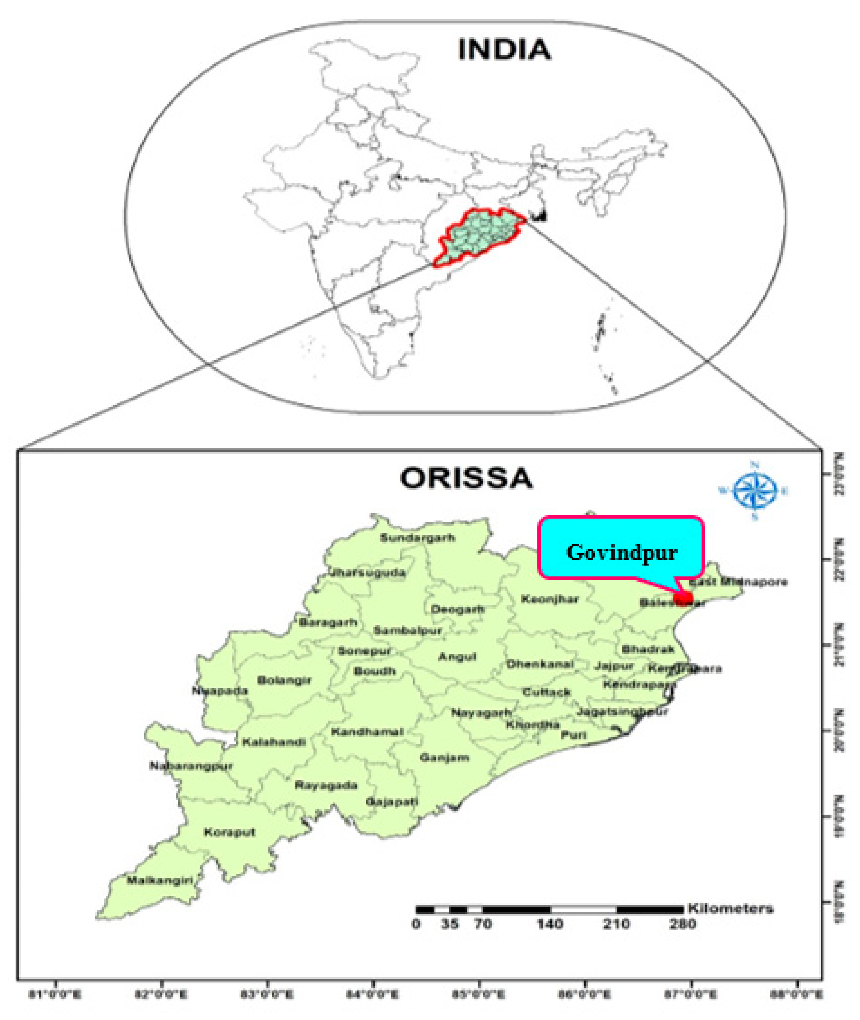
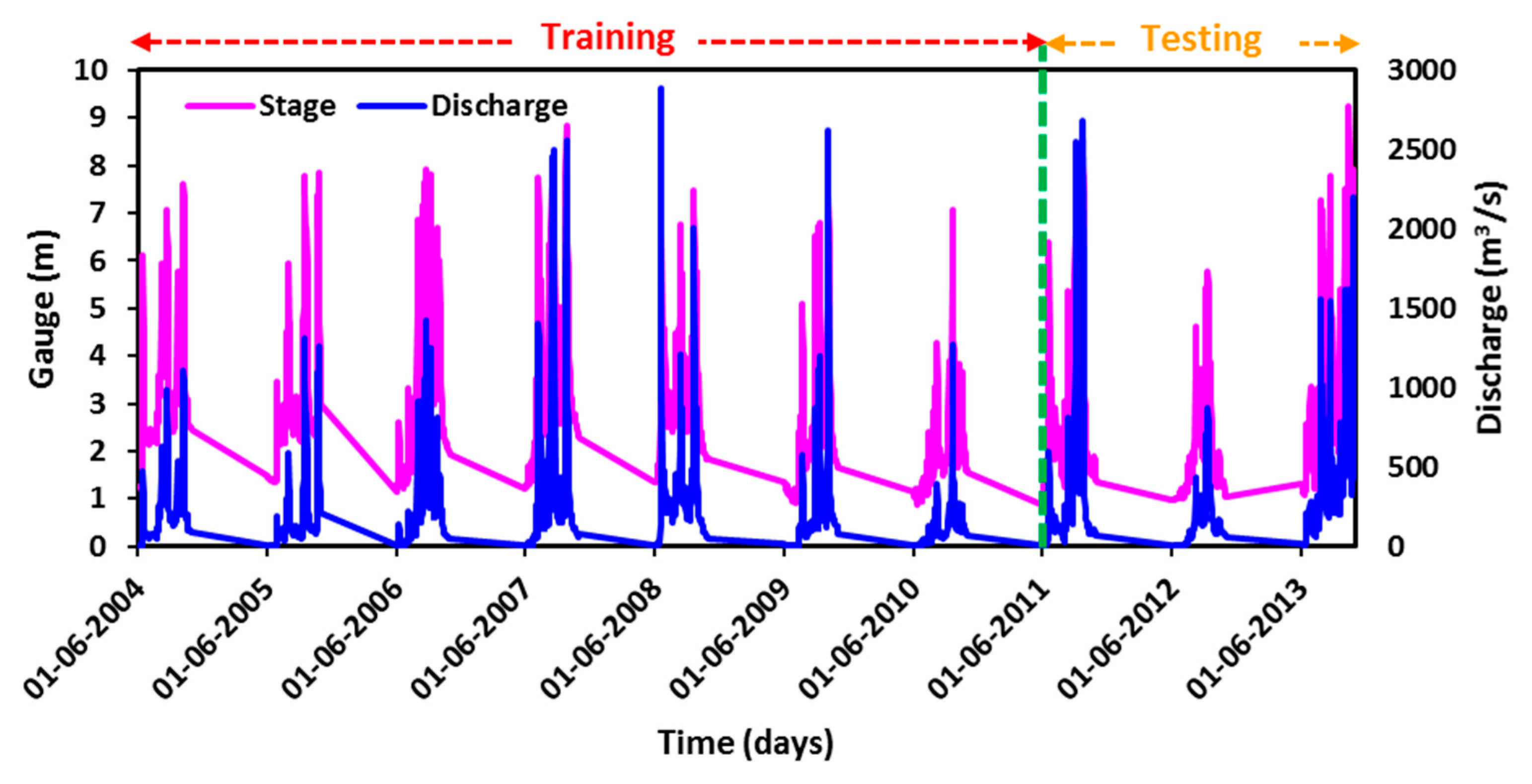
2.1. Study Area and Data Collection

The study area NH-5 road bridge Govindpur is commonly known as Govindpur, located in the Balasore district of Orissa State (India) with latitude 21°32′52” N and longitude 86°55′ 14” E. The study site is the mainstream of the Burhabalang river which is an east-flowing river and also a part of the Subarnarekha river basin located in Orissa State. The contributing area of the drainage basin is 4495 km2. Figure 1 illustrates the location map of the study area. The basin is strongly dominated by the south-west monsoon that starts in June and descends in mid-October. The average annual rainfall in the basin is about 1800 mm. The maximum temperature in the plains of the basin varies between 42 and 49 °C during May and goes down 8 to 14 °C during December–January. Geologically, the basin belongs mostly to Archean terrains. The rocks in the basin include Gneisses, Schist, Quartzite, and Amphibolite. Igneous rocks are also seen in the riverbed at some places.
The hydrological data including the daily stage (m) and discharge (m3/s) of 10 years (1st June 2004–31st October 2013) were obtained from the India-Water Resources Information System (WRIS) portal. The time series plot of the total available datasets of stage and discharge versus time is shown in Figure 2. The whole data were divided into two parts: (i) training dataset consisting of 70% (1st June 2004 to 31st October 2010) of the total data which were used for the development of the model, and (ii) remaining 30% (1st June 2011 to 31st October 2013) of the total data which were used for testing to check the prediction capability of the applied models (Figure 2). Figure 3 shows the relationship between stage and discharge through the rating curve at the study site. In contrast, Figure 4 illustrates the flowchart of the adopted methodology for discharge estimation at the Govindpur site.

2.2. Wavelet Transforms

Wavelet analysis (WA) is a promising time-frequency technique for signal processing with more advantages than Fourier analysis [14]. WA is an enhanced version of Fourier transformation used to detect time features in data [47,48]. Generally, discrete wavelet transformation (DWT) has been used for data decomposition which is advantageous over continuous wavelet transformation (CWT), so that CWT computes wavelet coefficients at every possible scale, which is time-consuming and also produces comprehensive data. DWT is better for analyzing. It reduces the scaling and shifting factors of the fundamental wavelet function to discrete values, maintaining analytical exactness. DWT was notably used in recent years as a computing tool to extract information on non-stationary signals [47,49,50].
The original discrete time-series C 0 ( t ) can be resolved by the Haar à trous decomposition algorithm [51] using Equations (1) and (2):
C r ( t ) = l = 0 + h ( l ) C r 1 ( t + 2 r ) ( r = 1 ,   2 ,   3 ,   ,   n )
W r ( t ) = C r 1 ( t ) C r ( t ) ( r = 1 ,   2 ,   3 ,   ,   n )
where h ( l ) is the discrete low-pass filter, and C r ( t ) and W r ( t ) (r = 1, 2, 3, …., n) are scale and wavelet coefficients at the resolution level. For detailed information regarding wavelet transformation, readers can refer to [52,53,54,55,56].
In the present study, the DWT method was employed for daily discharge estimation. The wavelet transform decomposes the original input time series data of stage and discharges into different frequencies. Three levels of the Haar à trous decomposition algorithm were used in this study. The new decomposed frequencies values act as input for the ANN. The hybridization of the decomposed wavelet value with ANN becomes a wavelet artificial neural network (WANN). The detailed information about ANN can be found in [57]. The Levenberg–Marquardt algorithm was utilized for the training of the model, and the hyperbolic tangent sigmoid transfer function was used to calculate a layer’s output from its net input.

2.3. Support Vector Machine (SVM)

Vapnik [58] developed the idea of a support vector machine (SVM). The SVM technology informs an excess glider from the input field that disintegrates a particular training dataset and permits distance on both sides of the hyperplane from the nearest instances. The data showing the maximum margin are referred to as support vectors during the regression analysis. These are the dataset points where approximate errors are equal to or greater than the available tube size of the SVM. There would be a non-linear separation between the training data. Then, it is necessary to construct a non-linear separable boundary. The mapping of the original space to a higher dimension is needed to create a non-linear boundary, and this is called the feature space. A kernel function defines the mapping of the feature space from a given input space. For optimization of the model, a penalty factor (c) has been introduced for misclassification. The total penalty in mapping is obtained by adding the penalties on each misclassification. Several useful applications of the SVM technique have been found in water resources engineering [59,60,61,62,63,64].
When the SVM algorithm is applied to classification problems, it is called support vector classification (SVC), and when applied to regression problems, it is called support vector regression (SVR) [65,66]. The use of kernel function makes this technique attractive, an excellent generalization, and applicable in the approximation of both linear and non-linear datasets. The lack of an optimal solution is due to the convex nature of the target function and its limitations. The SVM work based on the principle of structural risk minimization was carried out to mitigate the generalization rather than the training error. Consider a training dataset, T, represented using Equation (3):
T = { ( x 1 , y 1 ) , ( x 2 , y 2 ) , , ( x m , y m ) }
where x ϵ X ⸦ Rn are the training inputs and y ϵ, Y ⸦ Rn are the training outputs. Assume a non-linear function f ( x ) is given by Equation (4):
f ( x ) = w T ϕ ( x i ) + b
where w is the weight vector, b is the bias, and ϕ is a linearly mapped space with a high-dimensional function, x. Therefore, Equation (4) is transformed into a constrained complex optimization problem using Equations (5) and (6) as:
minimize : 1 2 w T w + c i = 1 m ( ξ i + ξ i * )
subject   to : { y i     ( w T Φ ( x i ) b )   ε + ξ i ( w T Φ ( x i ) + b ) y i   ε + ξ i * ξ i , ξ i * 0 ,     i = 1 ,   2 ,   , m
where   ξ i and   ξ i * are the loose (or slack) parameters, c (>0) is the penalty variable, and ε is the tube size that represents the maximum acceptable deviation. The Lagrangian multipliers are used to solve complex optimization problems [67,68]. The final expansion of SVM is defined using Equation (7) as [69]:
f ( x ) = i = 1 m ( a i + a i )   K ( x i , x j ) + b
where α i + and   α i are the Lagrangian multipliers, and K ( x i ,   x j ) is the kernel function. The kernel function of the SVM technique allows solving non-linear approximations into a linear function. The kernel functions used in this study were [69,70,71]:
  • Linear kernel function: the simplest type of kernel function and written by using Equation (8) [72]:
    K ( x i ,   x j ) = ( x i ,   x j )
  • Radial basis function (RBF): a mapping of RBF that is similar to Gaussian bell-shaped, and expressed by using Equation (9) [72]:
    K ( x i ,   x j ) = exp ( γ x i   x j 2 )
    where γ   is the width of the Gaussian RBF kernel parameter. The RBF is widely used among all the kernel functions in the SVM technique. The optimization of SVM in the training phase largely depends on c , γ , and ε parameters. This is because of outstanding features that can effectively tackle the linear and non-linear input-output mapping.

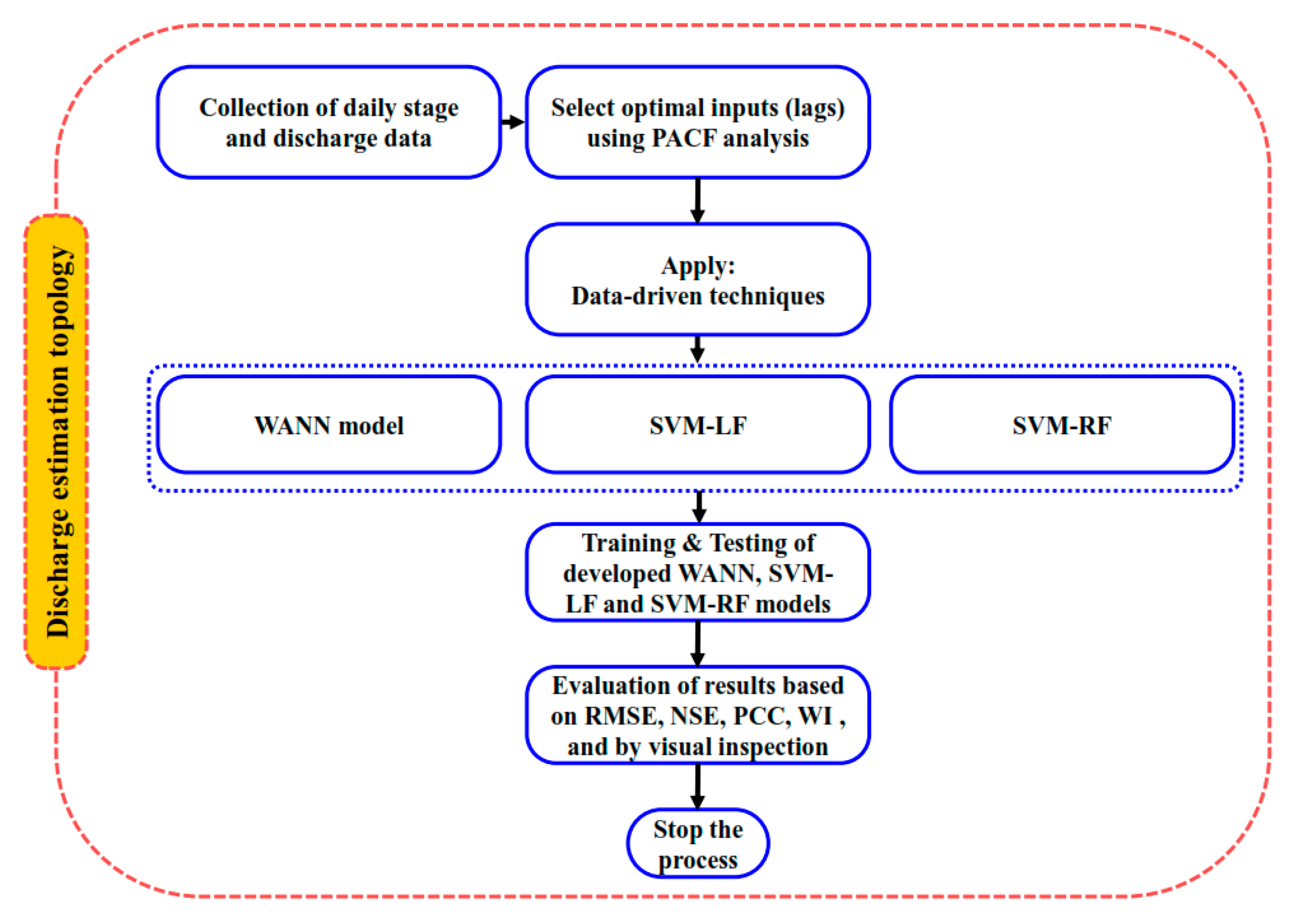
2.4. Model Development and Performance Indicators

The current day streamflow not only depends on the current day conditions but also on the previous days [73]. In this context, lagged input variables are very epochal in time series modeling. However, it is challenging to determine the optimal number of lagged input variables. PACF analysis gives a promising idea to select the optimal number of lags/inputs variables and regression of the time series against its past lagged value, served to remove any dependence on intermediate elements within lags [41,74,75,76]. In the present study, time-series data of discharge and stage have been lagged based on PACF analysis, so that the actual pattern of PACF among the data could be understood (Figure 5). It was observed that the first three days of lags from the present give more influence on discharge and stage at the 5% significance level. Based on this, lag 1, 2, and 3 from H and Q were selected, and the following three scenarios have been developed in Equations (10)–(12):
S c e n a r i o 1 : Q t = f ( H t ,   H t 1 ,   Q t 1 )
S c e n a r i o 2 : Q t = f ( H t ,   H t 1 ,   H t 2 ,   Q t 1 , Q t 2 )
S c e n a r i o 3 : Q t = f ( H t ,   H t 1 ,   H t 2 ,   H t 3 ,   Q t 1 , Q t 2 , Q t 3 )
Scenario 1 has a minimum number of inputs, viz., current-day stage, previous 1-day stage, and discharge (Equation (10)). Scenario 2 comprises the average number of inputs, viz., current-day stage, previous 1- and 2-days stage, and discharge (Equation (11)). Meanwhile, scenario 3 includes the maximum number of inputs, namely., current-day stage, previous 1-, 2-, and 3-days stage, and discharge (Equation (12)). All the models have been formulated to predict current day discharge (Qt) at the study site.
The performance of the scenarios mentioned above was evaluated statistically using root mean square error (RMSE), Nash–Sutcliffe efficiency (NSE), Pearson’s correlation coefficient (PCC), and the Willmott index (WI), and through graphical interpretation (time series plot, scatter plot, and Taylor diagram). The advantages and disadvantages of RMSE, NSE, PCC, and WI with definitions are discussed subsequently:
The RMSE measures the difference between observed and estimated values (Equation (13)). The RMSE reports in the same units as the model output and illustrates the size of a typical error. For continuous long-term simulation, RMSE performs well. The RMSE inclines to give more weight to high values than low values because errors in high values are generally more in absolute values than the errors in low values. The RMSE ranges from zero to infinite (0 < RMSE < ∞), so the lower the RMSE, the better the model performance [77,78].
NSE was initially proposed by Nash–Sutcliffe [79] and widely used to evaluate the hydrologic models [78,80,81]. It is the ratio of the mean square error to the variance of observed data during the period under examination, subtracted from unity (Equation (14)). The major limitation of NSE is that the differences between observed and estimated values are calculated as squared values. In other words, it cannot help to identify model bias, differences in magnitudes of peak flows, and the shape of recession curves. Similarly, it cannot be used for single-event simulation [78,80,81]. NSE ranges from minus infinity to one (−∞ < NSE < 1), so the closer to 1, the better the fit. An NSE lower than zero (NSE < 0) shows that the observed mean is as good a predictor as the model, while negative values specify that the observed mean is a better predictor than the model [78,80,81].
The PCC also is known as the correlation coefficient or coefficient of correlation used to measure the degree of collinearity between the observed and estimated variables in hydrological studies [78,81]. The PCC is oversensitive to extreme values and insensitive to additive and proportional variances among model predictions and observed data [81,82]. The PCC varies from minus one to plus one (−1 < PCC < 1), so close to one means a perfect fit (Equation (15)).
The WI, also known as the index of agreement, was developed by Willmott [83] to overcome the insensitivity of NSE and the coefficient of determination (R2) to the differences in observed and estimated means and variances [81,82]. It represents the ratio of the mean square error and the potential error [83]. The WI varies between zero and one (0 < WI ≤ 1), so near to 1 means a perfect agreement/fit, while approaching 0 means complete disagreements between the observed and estimated data (Equation (16)). The main disadvantages of WI are over-sensitivity to extremes values due to the squared differences. The high values of WI were reported even for poor model fits [81,82].
Finally, the RMSE [31,69,77,78], NSE [79], PCC [38,78,81,84], and WI [83] are written as
R M S E = 1 N   i = 1 N ( Q o b s , i     Q e s t , i ) 2 ( 0 < RMSE < )
N S E = 1 [ i = 1 N ( Q o b s , i     Q e s t , i ) 2 i = 1 N ( Q o b s , i     Q o b s   ¯ ) 2 ]
P C C = i = 1 N ( Q o b s , i     Q o b s   ¯ ) ( Q e s t , i     Q e s t ¯ )   i = 1 N ( Q o b s , i     Q o b s   ¯ ) 2 i = 1 N ( Q e s t , i     Q e s t ¯ ) 2 ( 1 < PCC < 1 )
WI = 1 [ i = 1 N ( Q e s t , i     Q o b s , i ) 2 i = 1 N ( | Q e s t , i     Q o b s   ¯ | + | Q o b s , i     Q o b s   ¯ | ) 2 ]
where N is the data points, Q o b s   and Q e s t are the observed and estimated discharge values for ith observations, and Q o b s   ¯ and Q e s t   ¯ are the means of the observed and estimated discharge values.

3. Results and Discussion

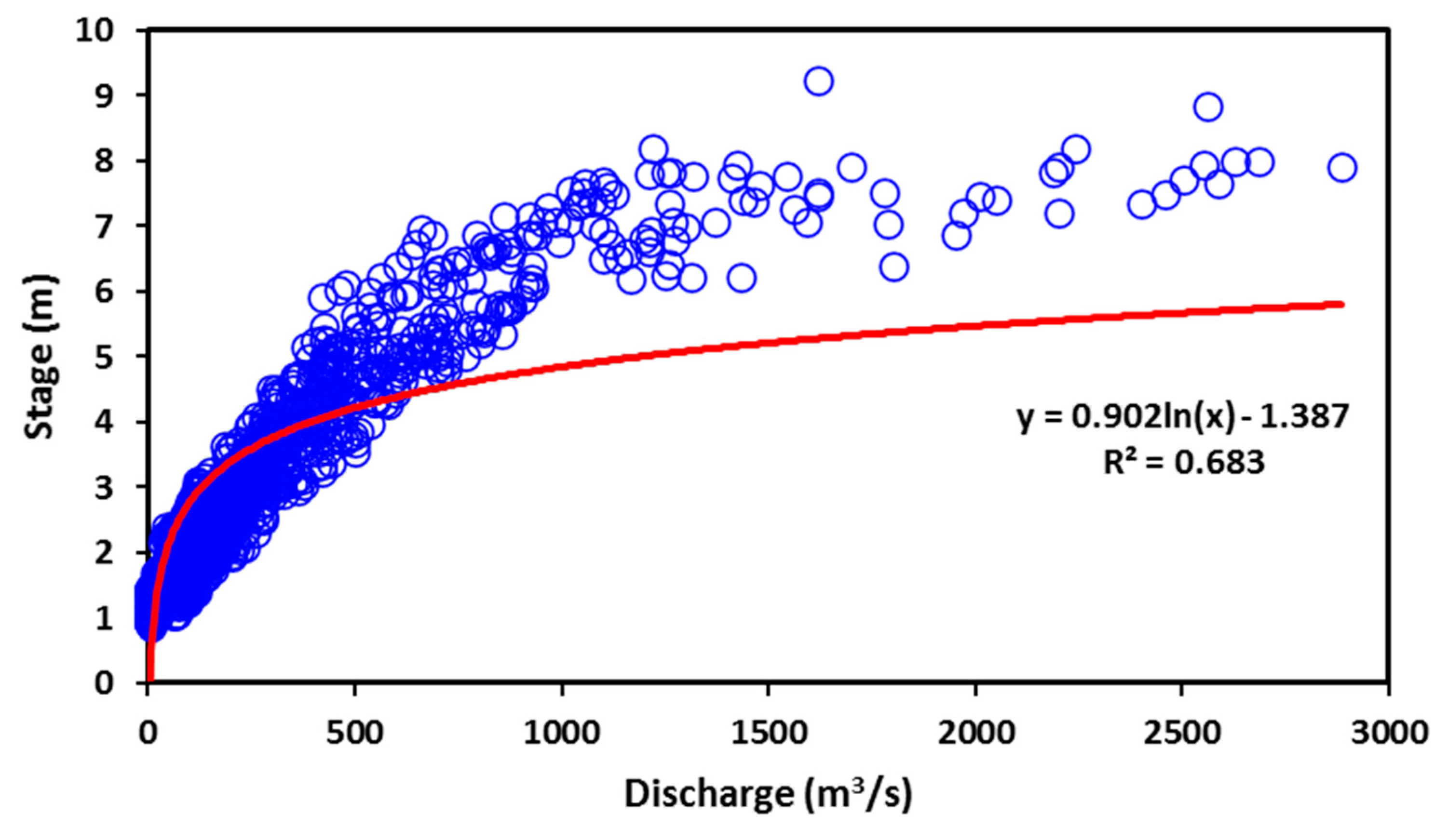
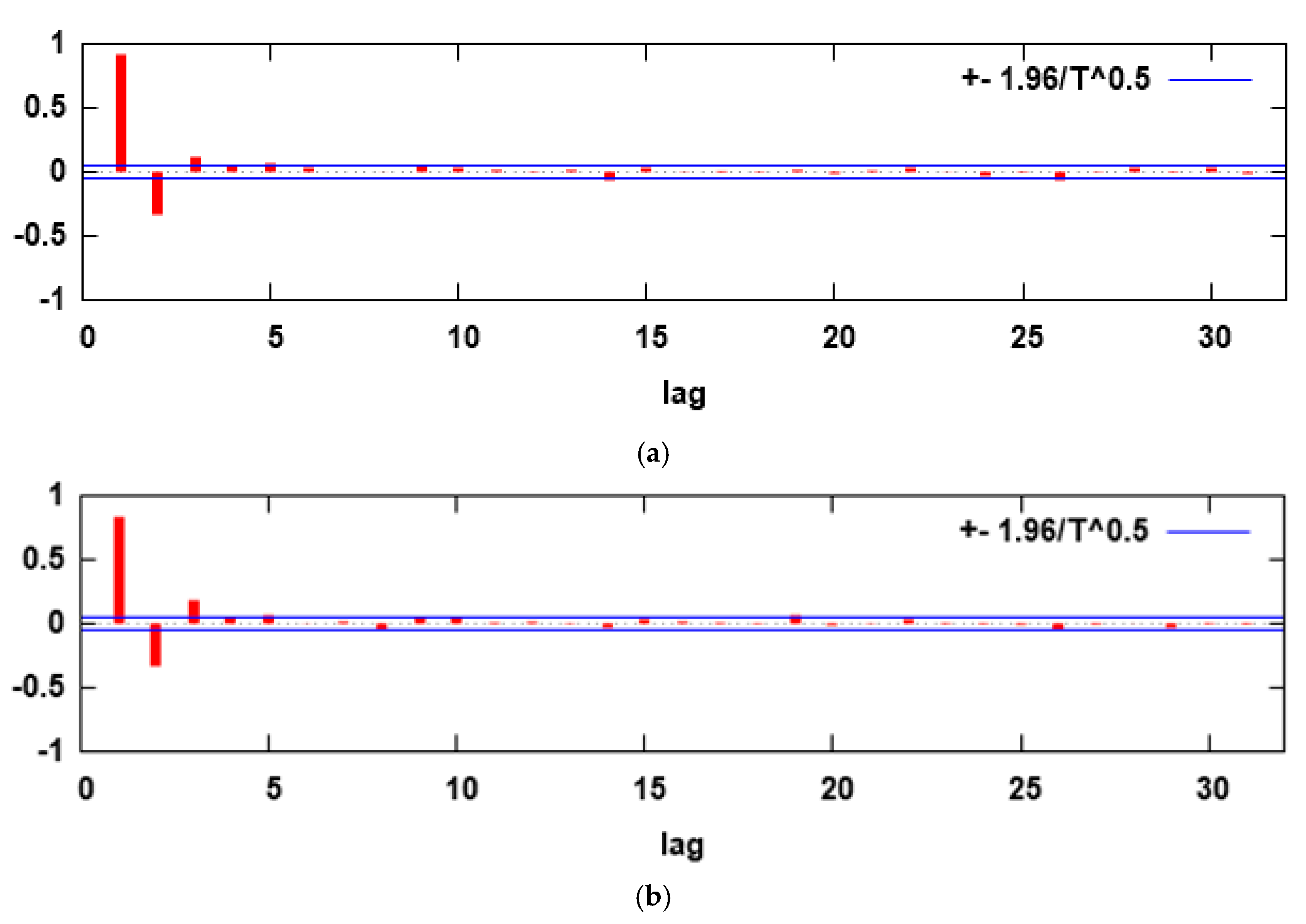
3.1. Statistical Analysis

The statistical analysis of stage (H) and discharge (Q) datasets for training, testing, and the entire period is given in Table 1, which includes various statistical parameters like mean, median, minimum and maximum value, standard deviation (Std. Dev.), coefficient of variation (CV), and skewness. These statistical parameters show the variability of data over time. When dividing the dataset into training and testing subsets, it is necessary to cross-validate the data to have the same statistical population. Due to the high skewness coefficient, there has been a considerable negative effect on model performance. Therefore, skewness coefficients are low for both calibration (1.3012) and validation (1.3441) sets for the given station. This is appropriate for discharge estimation at the study site. The standard deviation for the datasets shows that the values that are farther from zero mean that the variability in the data is higher. Hence, the variation of data from the mean value is higher.

3.2. Evaluation of Results from Various Trails

In the selection process of the best model, several trails have been performed on a single output. The trails of WANN were performed based on the different number of neurons in hidden layers. In contrast, trails of SVM-LF and SVM-RF were performed by taking several values of SVM-g, SVM-c, and SVM-e parameters from scenarios 1 to 3. The best four trails have been listed in Table 2, Table 3 and Table 4 based on testing results. The results of trail-2, trail-1, and trail-4 of WANN-1, SVM-LF-1, and SVM-RF-1 (Table 2); trail-3, trail-2, and trail-4 of WANN-2, SVM-LF-2, and SVM-RF-2 (Table 3); and trail-2 of WANN-3, SVM-LF-3, and SVM-RF-3 (Table 4) were found to be more promising than the other trails. Out of these trails, a total of nine have been imposed based on techniques and input selections and further evaluated to find the optimal one for daily discharge estimation at the study site (Table 5).

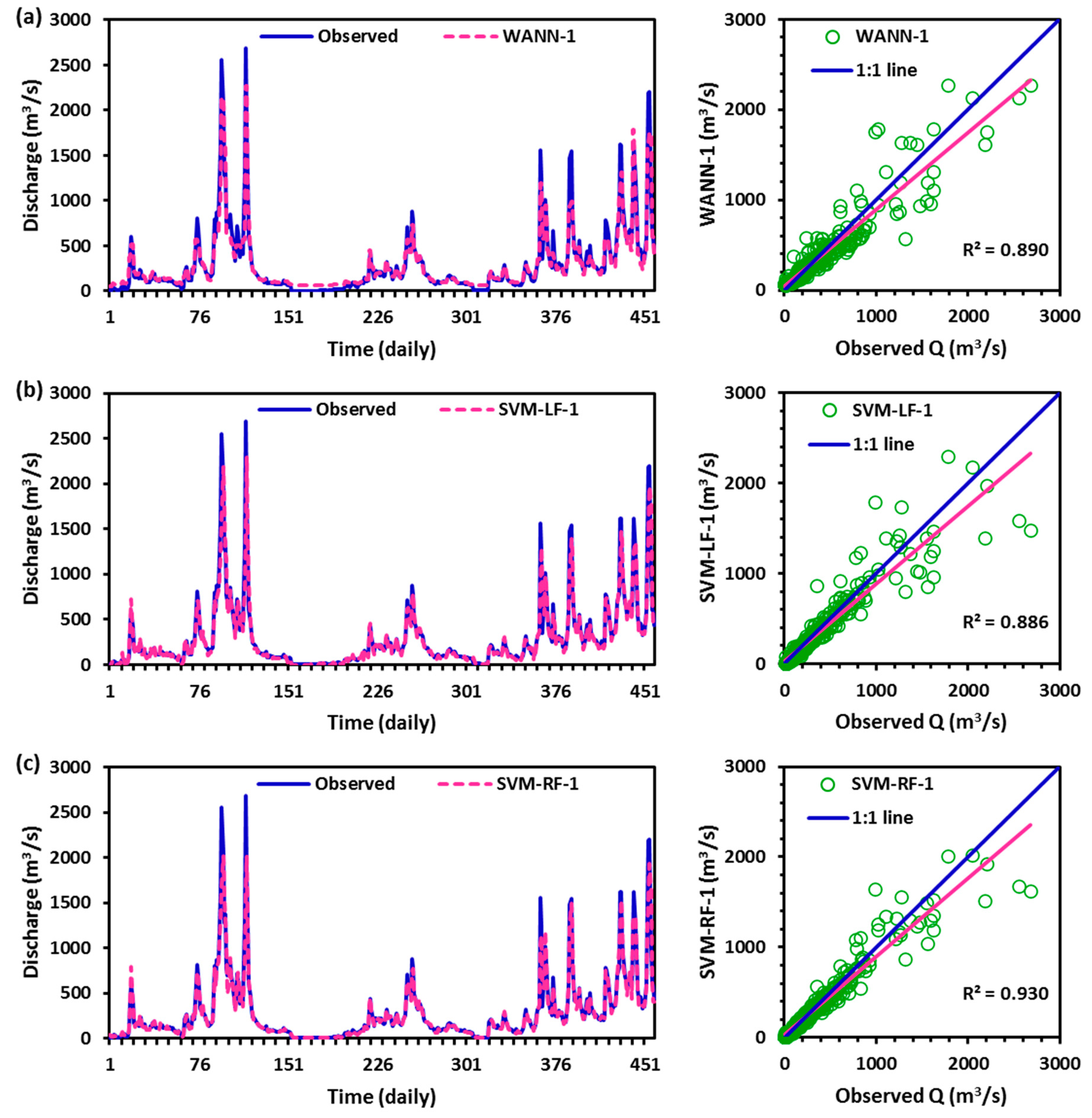
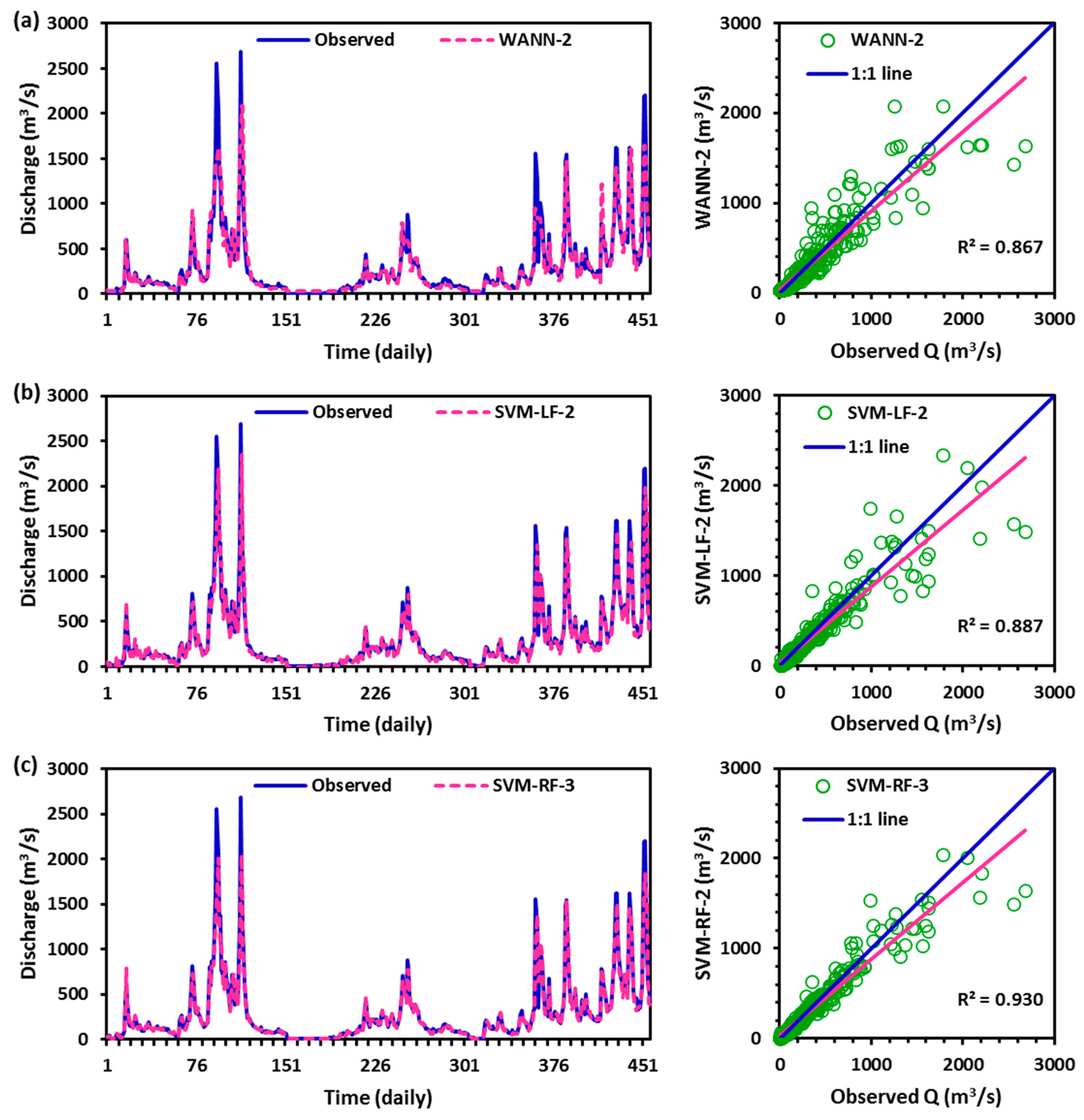
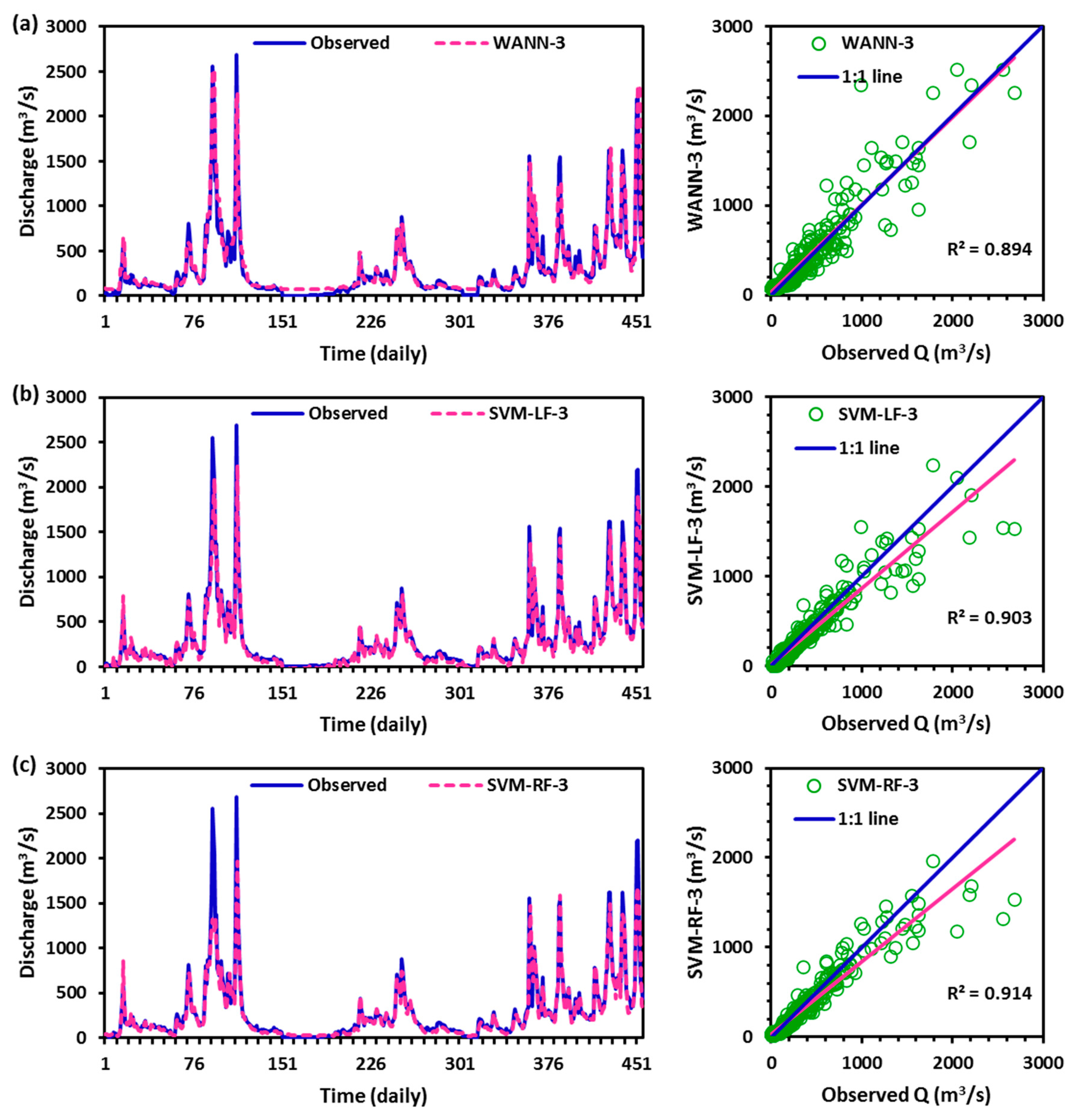
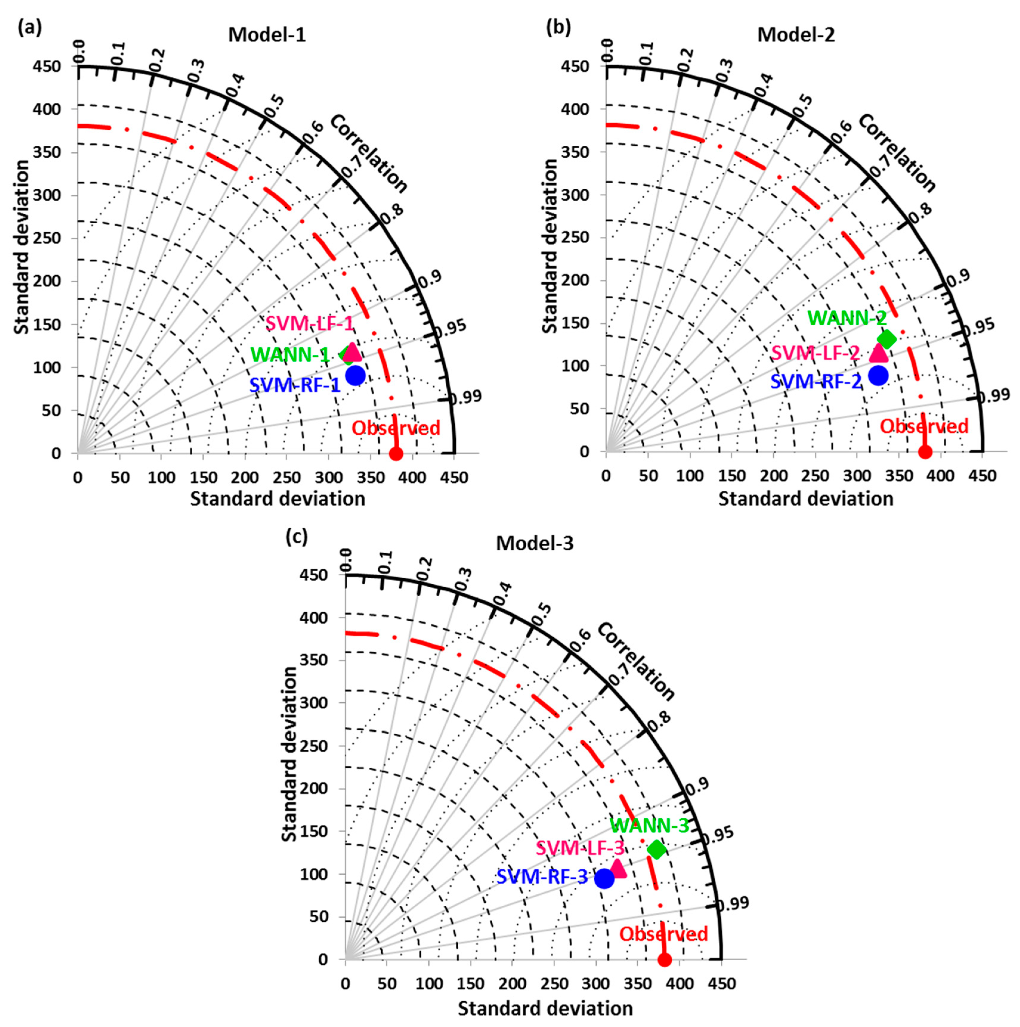
3.3. Quantitative and Qualitative Evaluation of Results

The RMSE, NSE, PCC, and WI values of all of the nine screened models over scenario 1 (S-1), scenario 2 (S-2), and scenario 3 (S-3) are given in Table 5. The model performance was classified as very good (PCC > 0.95, NSE > 0.80), good (0.85 ≤ PCC ≤ 0.95, 0.70 ≤ NSE ≤ 0.80), satisfactory (0.70 ≤ PCC ≤ 0.85, 0.50 ≤ NSE ≤ 0.70), and unsatisfactory (PCC ≤ 0.70, NSE ≤ 0.50), as stated by Moriasi et al. [78], Kouchi et al. [85], and Paul and Negahban-Azar, [86]. After considering all the techniques’ best trails from three scenarios (S-1 to S-3), it was noted that the SVM-RF model performed better than the WANN and SVM-LF models based on quantitative performance evaluation indicators. It was also observed that the performance of the SVM-RF model was reduced as the input variables were increased. The values of RMSE (m3/s), NSE, PCC, and WI were obtained as 104.426, 0.925, 0.964, and 0.979, respectively, for SVM-RF-1, 106.594, 0.922, 0.964, and 0.978 for SVM-RF-2, and 122.262, 0.897, 0.956, and 0.969 for SVM-RF-3. The order of model performance based on NSE from very good to unsatisfactory was attained as SVM-RF-1 (0.925) > SVM-RF-2 (0.922) > SVM-RF-3 (0.897) > SVM-LF-3 (0.893) > WANN-1 (0.888) > SVM-LF-1 (0.883) = SVM-LF-2 (0.883) = WANN-3 (0.883) > WANN-2 (0.866). The order of model performance on the basis of the RMSE from best to inferior was obtained as SVM-RF-1 (104.426) > SVM-RF-2 (106.594) > SVM-RF-3 (122.262) > SVM-LF-3 (124.954) > WANN-1 (127.349) > SVM-LF-1 (130.404) > WANN-3 (130.441) > SVM-LF-2 (130.556) > WANN-2 (139.559). The order of model performance based on the WI from best to inferior was found as SVM-RF-1 (0.979) > SVM-RF-2 (0.978) > WANN-3 (0.971) > SVM-LF-3 (0.970) > SVM-RF-3 (0.969) > WANN-1 (0.968) > SVM-LF-1 (0.967) = SVM-LF-2 (0.967) > WANN-2 (0.963). The comparison of results in Table 5 confirmed the superiority of the SVM-RF model with M-1 (inputs H t ,   H t 1 ,   Q t 1 ) having the lowest value of RMSE = 104.426 m3/s, and the highest values of NSE = 0.925, PCC = 0.964, and WI = 0.979, closely followed by the SVM-RF-2 model.
The results of the optimal nine models in three different scenarios were plotted between observed and estimated discharge values in the form of time variation and scatter plots through Figure 6, Figure 7 and Figure 8. It was noted that from these figures the high discharge values are under-estimated (>180 m3/s), whereas low discharge (<180 m3/s) values are over-estimated by WANN, SVM-LF, and SVM-RF models during the testing period. The quantity of explained variation out of the total variation (R2: coefficient of determination) was obtained as excellent for SVM-RF-1 and SVM-RF-2 models. Based on R2 values, the order of the model performance from very satisfactory to unsatisfactory [87] was found as SVM-RF-1 (0.930) = SVM-RF-2 (0.930) > SVM-RF-3 (0.914) > SVM-LF-3 (0.903) > WANN-3 (0.894) > WANN-1 (0.890) > SVM-LF-2 (0.887) > SVM-LF-1 (0.886) > WANN-2 (0.867).
Figure 9a–c demonstrates the Taylor diagrams of WANN, SVM-LF, and SVM-RF corresponding to S-1, S-2, and S-3 during the testing period at the study site. The concept of the Taylor diagram was given by Taylor [88] to represent the spatial distribution of estimated values (i.e., test field) concerning the observed (reference field) by compiling the RMSE, standard deviation, and correlation coefficient in the polar system. It can be seen from these figures that the SVM-RF model is close to the observed (reference) field. Moreover, the SVM-RF-1 model has the lowest RMSE, less standard deviation, and a higher correlation in comparison to other models, and is nominated as an optimal model for daily discharge estimation with H t ,   H t 1 ,   Q t 1 inputs at the study site.
Further, to support the finding of this study, the results were compared with the recent literature [89,90,91,92,93,94]. Adnan et al. [95] applied the group method of data handling-neural network (GMDH-NN), dynamic evolving neural-fuzzy inference system (DENFIS), and multivariate adaptive regression splines (MARS) for monthly streamflow prediction at the Kalam and Chakdara stations of the Swat river basin, Pakistan. They found better performance of the DENFIS at the Kalam site (RMSE = 18.9 m3/s, MAE = 13.1 m3/s, NSE = 0.94), and MARS at the Chakdara site (RMSE = 47.5 m3/s, MAE = 31.6 m3/s, NSE = 0.91). Ali and Shahbaz [96] evaluated the performance of an ANN for daily streamflow prediction in the Jhelum river basin, Pakistan. The results of the analysis revealed the better suitability of ANN in daily streamflow prediction with RMSE = 127.70 m3/s, PCC = 0.98, and NSE = 0.96 during the testing period. Mohammadi et al. [97] predicted the monthly streamflow of the Vu Gia Thu Bon river (Vietnam) using a standalone ANFIS and hybrid ANFIS coupled with the shuffled frog leaping algorithm (ANFIS-SFLA). The results of the perusal displayed the superior performance of the ANFIS-SFLA model with RMSE = 141.39 m3/s, NSE = 0.88, and PCC = 0.88 over the ANFIS model (RMSE = 167.81 m3/s, NSE = 0.83, PCC = 0.83). Mohammadi et al. [98] applied classical MLP and their hybrid integrated with particle swarm (MLP-PSO), PSO-multi-verse optimizer (MLP-PSO-MVO), and bi-linear (MLP-BL) to predict the daily streamflow at four stations, i.e., Brantford and Galt located in Grand River, Canada, and Macon and Elkton positioned in Ocmulgee and Umpqua rivers, United States. The results of the comparison revealed that the MLP-BL models (RMSE = 6.426/ 6.067/ 24.441/ 34.535 m3/s, MAE = 3.530/ 3.190/ 11.825/ 14.878 m3/s, and R2 = 0.994/ 0.990/ 0.990/ 0.986) outperformed the other models at the Brantford, Galt, Macon, and Elkton stations, respectively. Tripura et al. [99] forecasted hourly streamflow of Barak riven basin, Assam (India) by employing the standalone co-active neuro-fuzzy inference system (CANFIS) and a hybrid of CANFIS optimized with the genetic algorithm (CANFIS-GA) and firefly algorithm (CANFIS-FA). They found that the CANFIS-FA model provides better results than the other models. The results of these studies support the application of artificial intelligence (AI) techniques in monthly and daily streamflow/discharge prediction. Likewise, the results of the current research are in fair agreement with the utility of the SVM-RF technique for daily discharge prediction at Govindpur station.

4. Conclusions

Prediction of discharge on daily, weekly, and monthly timescales is vital for short- and long-term water resources management, particularly in extreme events like floods and drought. Thus, the present study was projected to predict the daily stage-discharge relationship at Govindpur station located at the Burhabalang river basin, Orissa (India), by employing wavelet-based artificial neural networks (WANN) and a support vector machine (SVM) optimized with linear and radial basis kernel functions. The PACF analysis gives an appropriate idea to select the optimum numbers on input variables in time series-based modeling. Data with more variability have been chosen for training, and remaining data have been utilized to test the model performance. Based on performance indicators and by visual inspection, the results revealed that the SVM-RF model with H t ,   H t 1 ,   Q t 1 inputs perform superior to the WANN and SVM-LF models for daily discharge estimation during monsoon season at the study site. Also, it was noted that as the input variable increases, the computation process becomes more difficult, time-consuming, and sometimes produces inferiority in the results. The best performance of the SVM-RF technique can help researchers to use highly variable discharge data for such modeling in the future. Researchers are also suggested to take as many trails as possible to avoid any bias and related problems of over- and under-estimation for highly variable data.

Author Contributions

Conceptualization, M.K., D.P.K. and A.M.; methodology, M.K. and A.K. (Anuradha Kumari); software, M.K.; validation, M.K., A.K. (Anuradha Kumari), P.K., D.P.K. and A.M.; formal analysis, M.K. and A.M.; investigation, M.K., A.K. (Anuradha Kumari), D.P.K., P.K., A.M., R.A. and A.K. (Alban Kuriqi); writing—original draft preparation, M.K., A.K. (Anuradha Kumari), D.P.K., P.K., A.M., R.A. and A.K. (Alban Kuriqi); writing—review and editing, M.K., A.K. (Anuradha Kumari), D.P.K., P.K., A.M., R.A. and A.K. (Alban Kuriqi); visualization, P.K., A.M. and A.K. (Alban Kuriqi); supervision, P.K., A.M. and A.K. (Alban Kuriqi); project administration, A.K. (Alban Kuriqi); funding acquisition, A.K. (Alban Kuriqi). All authors have read and agreed to the published version of the manuscript.

Funding

This research received no external funding.

Acknowledgments

The authors appreciate the comments of anonymous reviewers which helped to improve this paper further. Alban Kuriqi was supported by a Ph.D. scholarship granted by Fundação para a Ciência e a Tecnologia, I.P. (FCT), Portugal, under the Ph.D. Program FLUVIO–River Restoration and Management, grant number PD/BD/114558/2016.

Conflicts of Interest

The authors declare no conflict of interest.

References

  1. Gericke, O.J.; Smithers, J.C. Review of methods used to estimate catchment response time for the purpose of peak discharge estimation. Hydrol. Sci. J. 2014, 59, 1935–1971. [Google Scholar] [CrossRef]
  2. Mohanty, P.K.; Mohanty, L.P.; Khatua, K.K. Discharge estimation in wide meandering compound channels. ISH J. Hydraul. Eng. 2019, 25, 1–15. [Google Scholar] [CrossRef]
  3. Schmidt, A.R.; Garcia, M.H. Theoretical Examination of Historical Shifts and Adjustments to Stage-Discharge Rating Curves. In Proceedings of the World Water & Environmental Resources Congress 2003, American Society of Civil Engineers, Reston, VA, USA, 23–26 June 2003; pp. 1–10. [Google Scholar]
  4. Schmidt, A.R.; Yen, B.C. Theoretical Development of Stage-Discharge Ratings for Subcritical Open-Channel Flows. J. Hydraul. Eng. 2008, 134, 1245–1256. [Google Scholar] [CrossRef]
  5. Ardıçlıoğlu, M.; Kuriqi, A. Calibration of channel roughness in intermittent rivers using HEC-RAS model: Case of Sarimsakli creek, Turkey. SN Appl. Sci. 2019, 1, 1080. [Google Scholar] [CrossRef] [Green Version]
  6. Manfreda, S.; Pizarro, A.; Moramarco, T.; Cimorelli, L.; Pianese, D.; Barbetta, S. Potential advantages of flow-area rating curves compared to classic stage-discharge-relations. J. Hydrol. 2020, 585, 124752. [Google Scholar] [CrossRef]
  7. Westerberg, I.; Guerrero, J.-L.; Seibert, J.; Beven, K.J.; Halldin, S. Stage-discharge uncertainty derived with a non-stationary rating curve in the Choluteca River, Honduras. Hydrol. Process. 2011, 25, 603–613. [Google Scholar] [CrossRef]
  8. Petersen-Øverleir, A. Modelling stage—Discharge relationships affected by hysteresis using the Jones formula and nonlinear regression. Hydrol. Sci. J. 2006, 51, 365–388. [Google Scholar] [CrossRef] [Green Version]
  9. Rojas, M.; Quintero, F.; Young, N. Analysis of Stage–Discharge Relationship Stability Based on Historical Ratings. Hydrology 2020, 7, 31. [Google Scholar] [CrossRef]
  10. Kuriqi, A.; Ardiçlioǧlu, M. Investigation of hydraulic regime at middle part of the Loire River in context of floods and low flow events. Pollack Period. 2018, 13, 145–156. [Google Scholar] [CrossRef]
  11. Kuriqi, A.; Koçileri, G.; Ardiçlioğlu, M. Potential of Meyer-Peter and Müller approach for estimation of bed-load sediment transport under different hydraulic regimes. Model. Earth Syst. Environ. 2020, 6, 129–137. [Google Scholar] [CrossRef]
  12. Ghorbani, M.A.; Deo, R.C.; Kim, S.; Hasanpour Kashani, M.; Karimi, V.; Izadkhah, M. Development and evaluation of the cascade correlation neural network and the random forest models for river stage and river flow prediction in Australia. Soft Comput. 2020, 24, 12079–12090. [Google Scholar] [CrossRef]
  13. Bhattacharya, B.; Solomatine, D.P. Neural networks and M5 model trees in modelling water level–discharge relationship. Neurocomputing 2005, 63, 381–396. [Google Scholar] [CrossRef]
  14. Adamowski, J.; Fung Chan, H.; Prasher, S.O.; Ozga-Zielinski, B.; Sliusarieva, A. Comparison of multiple linear and nonlinear regression, autoregressive integrated moving average, artificial neural network, and wavelet artificial neural network methods for urban water demand forecasting in Montreal, Canada. Water Resour. Res. 2012, 48, W01528. [Google Scholar] [CrossRef]
  15. Aggarwal, S.K.; Goel, A.; Singh, V.P. Stage and Discharge Forecasting by SVM and ANN Techniques. Water Resour. Manag. 2012, 26, 3705–3724. [Google Scholar] [CrossRef]
  16. Kalteh, A.M. Monthly river flow forecasting using artificial neural network and support vector regression models coupled with wavelet transform. Comput. Geosci. 2013, 54, 1–8. [Google Scholar] [CrossRef]
  17. Supharatid, S. Application of a neural network model in establishing a stage-discharge relationship for a tidal river. Hydrol. Process. 2003, 17, 3085–3099. [Google Scholar] [CrossRef]
  18. Londhe, S.; Panse-Aglave, G. Modelling Stage–Discharge Relationship using Data-Driven Techniques. ISH J. Hydraul. Eng. 2015, 21, 207–215. [Google Scholar] [CrossRef]
  19. Deka, P.; Chandramouli, V. A fuzzy neural network model for deriving the river stage—Discharge relationship. Hydrol. Sci. J. 2003, 48, 197–209. [Google Scholar] [CrossRef] [Green Version]
  20. Lohani, A.K.; Goel, N.K.; Bhatia, K.K.S. Takagi–Sugeno fuzzy inference system for modeling stage–discharge relationship. J. Hydrol. 2006, 331, 146–160. [Google Scholar] [CrossRef]
  21. Alizadeh, F.; Faregh Gharamaleki, A.; Jalilzadeh, R. A two-stage multiple-point conceptual model to predict river stage-discharge process using machine learning approaches. J. Water Clim. Chang. 2020, 11, 1–18. [Google Scholar] [CrossRef]
  22. Roushangar, K.; Foroudi Khowr, A.; Saneie, M. Experimental study and artificial intelligence-based modeling of discharge coefficient of converging ogee spillways. ISH J. Hydraul. Eng. 2019, 25, 1–8. [Google Scholar] [CrossRef]
  23. Norouzi, R.; Daneshfaraz, R.; Ghaderi, A. Investigation of discharge coefficient of trapezoidal labyrinth weirs using artificial neural networks and support vector machines. Appl. Water Sci. 2019, 9, 148. [Google Scholar] [CrossRef]
  24. Najah Ahmed, A.; Binti Othman, F.; Abdulmohsin Afan, H.; Khaleel Ibrahim, R.; Ming Fai, C.; Shabbir Hossain, M.; Ehteram, M.; Elshafie, A. Machine learning methods for better water quality prediction. J. Hydrol. 2019, 578, 124084. [Google Scholar] [CrossRef]
  25. Muharemi, F.; Logofătu, D.; Leon, F. Machine learning approaches for anomaly detection of water quality on a real-world data set. J. Inf. Telecommun. 2019, 3, 294–307. [Google Scholar] [CrossRef] [Green Version]
  26. Di, Z.; Chang, M.; Guo, P. Water Quality Evaluation of the Yangtze River in China Using Machine Learning Techniques and Data Monitoring on Different Time Scales. Water 2019, 11, 339. [Google Scholar] [CrossRef] [Green Version]
  27. Moon, S.-H.; Kim, Y.-H.; Lee, Y.H.; Moon, B.-R. Application of machine learning to an early warning system for very short-term heavy rainfall. J. Hydrol. 2019, 568, 1042–1054. [Google Scholar] [CrossRef]
  28. Bojang, P.O.; Yang, T.-C.; Pham, Q.B.; Yu, P.-S. Linking Singular Spectrum Analysis and Machine Learning for Monthly Rainfall Forecasting. Appl. Sci. 2020, 10, 3224. [Google Scholar] [CrossRef]
  29. Pham, Q.B.; Abba, S.I.; Usman, A.G.; Linh, N.T.T.; Gupta, V.; Malik, A.; Costache, R.; Vo, N.D.; Tri, D.Q. Potential of Hybrid Data-Intelligence Algorithms for Multi-Station Modelling of Rainfall. Water Resour. Manag. 2019, 33, 5067–5087. [Google Scholar] [CrossRef]
  30. Pour, S.H.; Wahab, A.K.A.; Shahid, S. Physical-empirical models for prediction of seasonal rainfall extremes of Peninsular Malaysia. Atmos. Res. 2020, 233, 104720. [Google Scholar] [CrossRef]
  31. Malik, A.; Kumar, A.; Ghorbani, M.A.; Kashani, M.H.; Kisi, O.; Kim, S. The viability of co-active fuzzy inference system model for monthly reference evapotranspiration estimation: Case study of Uttarakhand State. Hydrol. Res. 2019, 50, 1623–1644. [Google Scholar] [CrossRef] [Green Version]
  32. Alizamir, M.; Kisi, O.; Muhammad Adnan, R.; Kuriqi, A. Modelling reference evapotranspiration by combining neuro-fuzzy and evolutionary strategies. Acta Geophys. 2020, 68, 1113–1126. [Google Scholar] [CrossRef]
  33. Yamaç, S.S.; Todorovic, M. Estimation of daily potato crop evapotranspiration using three different machine learning algorithms and four scenarios of available meteorological data. Agric. Water Manag. 2020, 228, 105875. [Google Scholar] [CrossRef]
  34. Malik, A.; Kumar, A. Pan Evaporation Simulation Based on Daily Meteorological Data Using Soft Computing Techniques and Multiple Linear Regression. Water Resour. Manag. 2015, 29, 1859–1872. [Google Scholar] [CrossRef]
  35. Malik, A.; Kumar, A.; Kisi, O. Monthly pan-evaporation estimation in Indian central Himalayas using different heuristic approaches and climate based models. Comput. Electron. Agric. 2017, 143, 302–313. [Google Scholar] [CrossRef]
  36. Ashrafzadeh, A.; Malik, A.; Jothiprakash, V.; Ghorbani, M.A.; Biazar, S.M. Estimation of daily pan evaporation using neural networks and meta-heuristic approaches. ISH J. Hydraul. Eng. 2018, 24, 1–9. [Google Scholar] [CrossRef]
  37. Malik, A.; Kumar, A.; Kisi, O. Daily Pan Evaporation Estimation Using Heuristic Methods with Gamma Test. J. Irrig. Drain. Eng. 2018, 144, 04018023. [Google Scholar] [CrossRef]
  38. Malik, A.; Rai, P.; Heddam, S.; Kisi, O.; Sharafati, A.; Salih, S.Q.; Al-Ansari, N.; Yaseen, Z.M. Pan Evaporation Estimation in Uttarakhand and Uttar Pradesh States, India: Validity of an Integrative Data Intelligence Model. Atmosphere 2020, 11, 553. [Google Scholar] [CrossRef]
  39. Rahmati, O.; Falah, F.; Dayal, K.S.; Deo, R.C.; Mohammadi, F.; Biggs, T.; Moghaddam, D.D.; Naghibi, S.A.; Bui, D.T. Machine learning approaches for spatial modeling of agricultural droughts in the south-east region of Queensland Australia. Sci. Total Environ. 2020, 699, 134230. [Google Scholar] [CrossRef]
  40. Das, P.; Naganna, S.R.; Deka, P.C.; Pushparaj, J. Hybrid wavelet packet machine learning approaches for drought modeling. Environ. Earth Sci. 2020, 79, 221. [Google Scholar] [CrossRef]
  41. Malik, A.; Kumar, A.; Singh, R.P. Application of Heuristic Approaches for Prediction of Hydrological Drought Using Multi-scalar Streamflow Drought Index. Water Resour. Manag. 2019, 33, 3985–4006. [Google Scholar] [CrossRef]
  42. Malik, A.; Kumar, A.; Piri, J. Daily suspended sediment concentration simulation using hydrological data of Pranhita River Basin, India. Comput. Electron. Agric. 2017, 138, 20–28. [Google Scholar] [CrossRef]
  43. Malik, A.; Kumar, A.; Kisi, O.; Shiri, J. Evaluating the performance of four different heuristic approaches with Gamma test for daily suspended sediment concentration modeling. Environ. Sci. Pollut. Res. 2019, 26, 22670–22687. [Google Scholar] [CrossRef] [PubMed]
  44. Zounemat-Kermani, M.; Mahdavi-Meymand, A.; Alizamir, M.; Adarsh, S.; Yaseen, Z.M. On the complexities of sediment load modeling using integrative machine learning: Application of the great river of Loíza in Puerto Rico. J. Hydrol. 2020, 585, 124759. [Google Scholar] [CrossRef]
  45. Kisi, O.; Dailr, A.H.; Cimen, M.; Shiri, J. Suspended sediment modeling using genetic programming and soft computing techniques. J. Hydrol. 2012, 450–451, 48–58. [Google Scholar] [CrossRef]
  46. Kumar, D.; Pandey, A.; Sharma, N.; Flügel, W.-A. Daily suspended sediment simulation using machine learning approach. CATENA 2016, 138, 77–90. [Google Scholar] [CrossRef]
  47. Daubechies, I. The wavelet transform, time-frequency localization and signal analysis. IEEE Trans. Inf. Theory 1990, 36, 961–1005. [Google Scholar] [CrossRef] [Green Version]
  48. Rioul, O.; Vetterli, M. Wavelets and signal processing. IEEE Signal Process. Mag. 1991, 8, 14–38. [Google Scholar] [CrossRef] [Green Version]
  49. Kim, C.-K.; Kwak, I.-S.; Cha, E.-Y.; Chon, T.-S. Implementation of wavelets and artificial neural networks to detection of toxic response behavior of chironomids (Chironomidae: Diptera) for water quality monitoring. Ecol. Model. 2006, 195, 61–71. [Google Scholar] [CrossRef]
  50. Dash, P.K.; Majumder, I.; Nayak, N.; Bisoi, R. Point and Interval Solar Power Forecasting Using Hybrid Empirical Wavelet Transform and Robust Wavelet Kernel Ridge Regression. Nat. Resour. Res. 2020, 29, 2813–2841. [Google Scholar] [CrossRef]
  51. Wang, W.; Ding, J. Wavelet Network Model and Its Application to the Prediction of Hydrology. Nat. Sci. 2003, 1, 67–71. [Google Scholar]
  52. Bhardwaj, S.; Chandrasekhar, E.; Padiyar, P.; Gadre, V.M. A comparative study of wavelet-based ANN and classical techniques for geophysical time-series forecasting. Comput. Geosci. 2020, 138, 104461. [Google Scholar] [CrossRef]
  53. Graf, R.; Zhu, S.; Sivakumar, B. Forecasting river water temperature time series using a wavelet–neural network hybrid modelling approach. J. Hydrol. 2019, 578, 124115. [Google Scholar] [CrossRef]
  54. Ghazvinei, P.T.; Shamshirband, S.; Motamedi, S.; Hassanpour Darvishi, H.; Salwana, E. Performance investigation of the dam intake physical hydraulic model using Support Vector Machine with a discrete wavelet transform algorithm. Comput. Electron. Agric. 2017, 140, 48–57. [Google Scholar] [CrossRef]
  55. Zhou, F.; Liu, B.; Duan, K. Coupling wavelet transform and artificial neural network for forecasting estuarine salinity. J. Hydrol. 2020, 588, 125127. [Google Scholar] [CrossRef]
  56. Zhang, J.; Zhang, X.; Niu, J.; Hu, B.X.; Soltanian, M.R.; Qiu, H.; Yang, L. Prediction of groundwater level in seashore reclaimed land using wavelet and artificial neural network-based hybrid model. J. Hydrol. 2019, 577, 123948. [Google Scholar] [CrossRef]
  57. Haykin, S. Neural Networks—A Comprehensive Foundation, 2nd ed.; Prentice-Hall: Up Saddle River, NJ, USA, 1999; pp. 26–32. [Google Scholar]
  58. Vapnik, V.N. The Nature of Statistical Learning Theory; Springer: New York, NY, USA, 1995; p. 314. [Google Scholar]
  59. Asefa, T.; Kemblowski, M.; Urroz, G.; McKee, M. Support vector machines (SVMs) for monitoring network design. Ground Water 2005, 43, 413–422. [Google Scholar] [CrossRef]
  60. Raghavendra, N.S.; Deka, P.C. Support vector machine applications in the field of hydrology: A review. Appl. Soft Comput. 2014, 19, 372–386. [Google Scholar] [CrossRef]
  61. Hipni, A.; El-shafie, A.; Najah, A.; Karim, O.A.; Hussain, A.; Mukhlisin, M. Daily Forecasting of Dam Water Levels: Comparing a Support Vector Machine (SVM) Model With Adaptive Neuro Fuzzy Inference System (ANFIS). Water Resour. Manag. 2013, 27, 3803–3823. [Google Scholar] [CrossRef]
  62. Nguyen, L. Tutorial on support vector machine. Appl. Comput. Math. 2017, 6, 1–15. [Google Scholar]
  63. Misra, D.; Oommen, T.; Agarwal, A.; Mishra, S.K.; Thompson, A.M. Application and analysis of support vector machine based simulation for runoff and sediment yield. Biosyst. Eng. 2009, 103, 527–535. [Google Scholar] [CrossRef]
  64. Gholami, R.; Fakhari, N. Support Vector Machine: Principles, Parameters, and Applications. In Handbook of Neural Computation; Elsevier: Amsterdam, The Netherlands, 2017; pp. 515–535. [Google Scholar]
  65. Mohammadi, B.; Mehdizadeh, S. Modeling daily reference evapotranspiration via a novel approach based on support vector regression coupled with whale optimization algorithm. Agric. Water Manag. 2020, 237, 106145. [Google Scholar] [CrossRef]
  66. Banadkooki, F.B.; Ehteram, M.; Panahi, F.; Sammen, S.S.; Othman, F.B.; EL-Shafie, A. Estimation of total dissolved solids (TDS) using new hybrid machine learning models. J. Hydrol. 2020, 587, 124989. [Google Scholar] [CrossRef]
  67. Su, H.; Li, X.; Yang, B.; Wen, Z. Wavelet support vector machine-based prediction model of dam deformation. Mech. Syst. Signal Process. 2018, 110, 412–427. [Google Scholar] [CrossRef]
  68. Panahi, M.; Sadhasivam, N.; Pourghasemi, H.R.; Rezaie, F.; Lee, S. Spatial prediction of groundwater potential mapping based on convolutional neural network (CNN) and support vector regression (SVR). J. Hydrol. 2020, 588, 125033. [Google Scholar] [CrossRef]
  69. Tikhamarine, Y.; Malik, A.; Souag-Gamane, D.; Kisi, O. Artificial intelligence models versus empirical equations for modeling monthly reference evapotranspiration. Environ. Sci. Pollut. Res. 2020, 27, 30001–30019. [Google Scholar] [CrossRef]
  70. Zhang, X.; Wang, J.; Zhang, K. Short-term electric load forecasting based on singular spectrum analysis and support vector machine optimized by Cuckoo search algorithm. Electr. Power Syst. Res. 2017, 146, 270–285. [Google Scholar] [CrossRef]
  71. Ansari, H.R.; Gholami, A. An improved support vector regression model for estimation of saturation pressure of crude oils. Fluid Phase Equilib. 2015, 402, 124–132. [Google Scholar] [CrossRef]
  72. Han, D.; Chan, L.; Zhu, N. Flood forecasting using support vector machines. J. Hydroinform. 2007, 9, 267–276. [Google Scholar] [CrossRef]
  73. Cobaner, M.; Unal, B.; Kisi, O. Suspended sediment concentration estimation by an adaptive neuro-fuzzy and neural network approaches using hydro-meteorological data. J. Hydrol. 2009, 367, 52–61. [Google Scholar] [CrossRef]
  74. Deo, R.C.; Tiwari, M.K.; Adamowski, J.F.; Quilty, J.M. Forecasting effective drought index using a wavelet extreme learning machine (W-ELM) model. Stoch. Environ. Res. Risk Assess. 2017, 31, 1211–1240. [Google Scholar] [CrossRef]
  75. Malik, A.; Kumar, A.; Salih, S.Q.; Kim, S.; Kim, N.W.; Yaseen, Z.M.; Singh, V.P. Drought index prediction using advanced fuzzy logic model: Regional case study over Kumaon in India. PLoS ONE 2020, 15, e0233280. [Google Scholar] [CrossRef] [PubMed]
  76. Malik, A.; Kumar, A. Meteorological drought prediction using heuristic approaches based on effective drought index: A case study in Uttarakhand. Arab. J. Geosci. 2020, 13, 276. [Google Scholar] [CrossRef]
  77. Gan, T.Y.; Dlamini, E.M.; Biftu, G.F. Effects of model complexity and structure, data quality, and objective functions on hydrologic modeling. J. Hydrol. 1997, 192, 81–103. [Google Scholar] [CrossRef]
  78. Moriasi, D.N.; Wilson, B.N.; Douglas-Mankin, K.R.; Arnold, J.G.; Gowda, P.H. Hydrologic and Water Quality Models: Use, Calibration, and Validation. Trans. ASABE 2012, 55, 1241–1247. [Google Scholar] [CrossRef]
  79. Nash, J.E.; Sutcliffe, J.V. River flow forecasting through conceptual models part I—A discussion of principles. J. Hydrol. 1970, 10, 282–290. [Google Scholar] [CrossRef]
  80. Willmott, C.; Matsuura, K. Advantages of the mean absolute error (MAE) over the root mean square error (RMSE) in assessing average model performance. Clim. Res. 2005, 30, 79–82. [Google Scholar] [CrossRef]
  81. Krause, P.; Boyle, D.P.; Bäse, F. Comparison of different efficiency criteria for hydrological model assessment. Adv. Geosci. 2005, 5, 89–97. [Google Scholar] [CrossRef] [Green Version]
  82. Legates, D.R.; McCabe, G.J. Evaluating the use of “goodness-of-fit” Measures in hydrologic and hydroclimatic model validation. Water Resour. Res. 1999, 35, 233–241. [Google Scholar] [CrossRef]
  83. Willmott, C.J. On the validation of models. Phys. Geogr. 1981, 2, 184–194. [Google Scholar] [CrossRef]
  84. Malik, A.; Kumar, A.; Kim, S.; Kashani, M.H.; Karimi, V.; Sharafati, A.; Ghorbani, M.A.; Al-Ansari, N.; Salih, S.Q.; Yaseen, Z.M.; et al. Modeling monthly pan evaporation process over the Indian central Himalayas: Application of multiple learning artificial intelligence model. Eng. Appl. Comput. Fluid Mech. 2020, 14, 323–338. [Google Scholar] [CrossRef] [Green Version]
  85. Kouchi, D.H.; Esmaili, K.; Faridhosseini, A.; Sanaeinejad, S.H.; Khalili, D.; Abbaspour, K.C. Sensitivity of Calibrated Parameters and Water Resource Estimates on Different Objective Functions and Optimization Algorithms. Water 2017, 9, 384. [Google Scholar] [CrossRef] [Green Version]
  86. Paul, M.; Negahban-Azar, M. Sensitivity and uncertainty analysis for streamflow prediction using multiple optimization algorithms and objective functions: San Joaquin Watershed, California. Model. Earth Syst. Environ. 2018, 4, 1509–1525. [Google Scholar] [CrossRef]
  87. Shamseldin, A.Y. Application of a neural network technique to rainfall-runoff modelling. J. Hydrol. 1997, 199, 272–294. [Google Scholar] [CrossRef]
  88. Taylor, K.E. Summarizing multiple aspects of model performance in a single diagram. J. Geophys. Res. Atmos. 2001, 106, 7183–7192. [Google Scholar] [CrossRef]
  89. Singh, A.; Malik, A.; Kumar, A.; Kisi, O. Rainfall-runoff modeling in hilly watershed using heuristic approaches with gamma test. Arab. J. Geosci. 2018, 11, 261. [Google Scholar] [CrossRef]
  90. Tikhamarine, Y.; Souag-Gamane, D.; Kisi, O. A new intelligent method for monthly streamflow prediction: Hybrid wavelet support vector regression based on grey wolf optimizer (WSVR–GWO). Arab. J. Geosci. 2019, 12, 540. [Google Scholar] [CrossRef]
  91. Tikhamarine, Y.; Souag-Gamane, D.; Najah Ahmed, A.; Kisi, O.; El-Shafie, A. Improving artificial intelligence models accuracy for monthly streamflow forecasting using grey Wolf optimization (GWO) algorithm. J. Hydrol. 2020, 582, 124435. [Google Scholar] [CrossRef]
  92. Tikhamarine, Y.; Souag-Gamane, D.; Ahmed, A.N.; Sammen, S.S.; Kisi, O.; Huang, Y.F.; El-Shafie, A. Rainfall-runoff modelling using improved machine learning methods: Harris hawks optimizer vs. particle swarm optimization. J. Hydrol. 2020, 589, 125133. [Google Scholar] [CrossRef]
  93. Hussain, D.; Khan, A.A. Machine learning techniques for monthly river flow forecasting of Hunza River, Pakistan. Earth Sci. Inform. 2020, 13, 939–949. [Google Scholar] [CrossRef]
  94. Khatibi, R.; Ghorbani, M.A.; Naghshara, S.; Aydin, H.; Karimi, V. A framework for ‘Inclusive Multiple Modelling’ with critical views on modelling practices–Applications to modelling water levels of Caspian Sea and Lakes Urmia and Van. J. Hydrol. 2020, 587, 124923. [Google Scholar] [CrossRef]
  95. Adnan, R.M.; Liang, Z.; Parmar, K.S.; Soni, K.; Kisi, O. Modeling monthly streamflow in mountainous basin by MARS, GMDH-NN and DENFIS using hydroclimatic data. Neural Comput. Appl. 2020, 32, 1–19. [Google Scholar] [CrossRef]
  96. Ali, S.; Shahbaz, M. Streamflow forecasting by modeling the rainfall–streamflow relationship using artificial neural networks. Model. Earth Syst. Environ. 2020, 6, 1645–1656. [Google Scholar] [CrossRef]
  97. Mohammadi, B.; Linh, N.T.T.; Pham, Q.B.; Ahmed, A.N.; Vojteková, J.; Guan, Y.; Abba, S.; El-Shafie, A. Adaptive neuro-fuzzy inference system coupled with shuffled frog leaping algorithm for predicting river streamflow time series. Hydrol. Sci. J. 2020, 65, 1738–1751. [Google Scholar] [CrossRef]
  98. Mohammadi, B.; Ahmadi, F.; Mehdizadeh, S.; Guan, Y.; Pham, Q.B.; Linh, N.T.T.; Tri, D.Q. Developing Novel Robust Models to Improve the Accuracy of Daily Streamflow Modeling. Water Resour. Manag. 2020, 34, 3387–3409. [Google Scholar] [CrossRef]
  99. Tripura, J.; Roy, P.; Barbhuiya, A.K. Simultaneous streamflow forecasting based on hybridized neuro-fuzzy method for a river system. Neural Comput. Appl. 2020, 32, 1–13. [Google Scholar] [CrossRef]
Figure 1. Location Map of the Study Area.
Sustainability 12 07877 g001
Figure 2. Time Series Plot of Stage and Discharge Datasets at the Study Site.
Sustainability 12 07877 g002
Figure 3. Rating Curve of the Stage-Discharge Relationship at the Study Site.
Sustainability 12 07877 g003
Figure 4. Flowchart of Discharge Estimation Methodology at the Study Site.
Sustainability 12 07877 g004
Figure 5. Partial Autocorrelation Function Values of (a) Stage, and (b) Discharge at the Study Site.
Sustainability 12 07877 g005
Figure 6. Observed Versus Estimated Discharge of Best (a) WANN-1, (b) SVM-LF-1, and (c) SVM-RF-1 Models During the Testing Period at the Study Site.
Sustainability 12 07877 g006
Figure 7. Observed versus estimated discharge of best (a) WANN-2, (b) SVM-LF-2, and (c) SVM-RF-2 models during the testing period at the study site.
Sustainability 12 07877 g007
Figure 8. Observed Versus Estimated Discharge of Best (a) WANN-3, (b) SVM-LF-3, and (c) SVM-RF-3 Models During the Testing Period at the Study Site.
Sustainability 12 07877 g008
Figure 9. Taylor diagram of WANN, SVM-LF, and SVM-RF corresponding to (a) scenario 1, (b) scenario 2, and (c) scenario 3 during the testing period at the study site.
Sustainability 12 07877 g009
Table 1. Statistics of Stage and Discharge Variables During Training, Testing, and Entire Periods at the Study Station.
Statistical ParameterTrainingTestingEntire
H
(m)
Q
(m3/s)
H
(m)
Q
(m3/s)
H
(m)
Q
(m3/s)
Mean2.9461243.502.7548291.602.8887257.93
Median2.5200136.802.2000157.122.4900142.61
Minimum0.86001.36900.86003.57300.86001.3690
Maximum8.84002885.99.24002685.69.24002885.9
Std. Dev.1.5805349.151.7028381.481.6200359.71
CV0.53641.43390.61811.30820.56081.3946
Skewness1.30123.61331.34412.89991.30133.3629
Table 2. Performance Indicators of WANN-1, SVM-LF-1, and SVM-RF-1 Models During Testing at the Study Station.
ModelPerformance Indicators
RMSENSEPCCWI
WANN-1
Trail-1148.6620.8480.9240.959
Trail-2127.3490.8880.9440.968
Trail-3133.6950.8770.9380.968
Trail-4157.4870.8290.9270.960
SVM-LF-1
Trail-1130.4040.8830.9410.967
Trail-2217.5310.6740.9520.930
Trail-3135.2500.8740.9540.968
Trail-4180.6880.7750.9540.948
SVM-RF-1
Trail-1108.9200.9180.9610.977
Trail-2106.2270.9220.9630.978
Trail-3106.2270.9220.9630.978
Trail-4104.4260.9250.9640.979
Table 3. Performance Indicators of WANN-2, SVM-LF-2, and SVM-RF-2 Models During Testing at the Study Station.
ModelPerformance Indicators
RMSENSEPCCWI
WANN-2
Trail-1139.5970.8660.9310.962
Trail-2139.8390.8660.9330.961
Trail-3139.5590.8660.9310.963
Trail-4151.8360.8420.9350.963
SVM-LF-2
Trail-1206.8400.7060.9530.938
Trail-2130.5560.8830.9420.967
Trail-3135.9720.8730.9560.968
Trail-4174.2460.7910.9540.952
SVM-RF-2
Trail-1111.3560.9150.9620.975
Trail-2109.0050.9180.9620.977
Trail-3108.3760.9190.9630.977
Trail-4106.5940.9220.9640.978
Table 4. Performance Indicators of WANN-3, SVM-LF-3, and SVM-RF-3 Models During Testing at the Study Station.
ModelPerformance Indicators
RMSENSEPCCWI
WANN-3
Trail-1148.5610.8480.9250.961
Trail-2130.4410.8830.9450.971
Trail-3244.9840.5880.8240.901
Trail-4134.5260.8760.9390.968
SVM-LF-3
Trail-1128.3840.8870.9450.968
Trail-2124.9540.8930.9500.970
Trail-3139.6340.8660.9540.966
Trail-4173.2770.7940.9510.953
SVM-RF-3
Trail-1130.5890.8830.9510.964
Trail-2122.2620.8970.9560.969
Trail-3147.5990.8500.9390.952
Trail-4124.5960.8930.9540.968
Table 5. Comparison of Best Outputs of WANN, SVM-LF, and SVM-RF Models at the Study Station.
ModelStructure/ParameterPerformance Indicators
RMSENSEPCCWI
WANN-112-5-1127.3490.8880.9440.968
SVM-LF-1 γ = 0.330, ε = 0.100, c = 10130.4040.8830.9410.967
SVM-RF-1 γ = 0.160, ε = 0.010, c = 10104.4260.9250.9640.979
WANN-220-9-1139.5590.8660.9310.963
SVM-LF-2 γ = 0.1428, ε = 0.010, c = 10130.5560.8830.9420.967
SVM-RF-2 γ = 0.120, ε = 0.010, c = 10106.5940.9220.9640.978
WANN-328-5-1130.4410.8830.9450.971
SVM-LF-3 γ = 0.143, ε = 0.010, c = 10124.9540.8930.9500.970
SVM-RF-3 γ = 0.160, ε = 0.100, c = 10122.2620.8970.9560.969

