Review

Review of Nitrogen Compounds Prediction in Water Bodies Using Artificial Neural Networks and Other Models

1
Department of Civil Engineering, Faculty of Engineering, University of Malaya, Kuala Lumpur 50603, Malaysia
2
Department of Civil Engineering, College of Engineering, University Tenaga Nasional (UNITEN), Jalan Ikram-UNITEN, Kajang 43000, Selangor, Malaysia
3
Institute for Sustainable Energy (ISE), University Tenaga Nasional (UNITEN), Kajang 43000, Selangor, Malaysia
4
Department of Biological and Agricultural Engineering, Faculty of Engineering, University Putra Malaysia, Selangor 43400, Malaysia
5
Department of Civil Engineering, Al-Maaref University College, Ramadi 31001, Iraq
6
Institute for Energy Infrastructure (IEI), University Tenaga Nasional (UNITEN), Kajang 43000, Selangor, Malaysia
7
Civil and Environmental Eng. Dept., College of Engineering, United Arab Emirates University, Al Ain 15551, UAE
8
National Water Center, United Arab Emirate University, Al Ain P.O. Box 15551, UAE
*
Author to whom correspondence should be addressed.
Sustainability 2020, 12(11), 4359; https://doi.org/10.3390/su12114359
Submission received: 22 April 2020 / Revised: 21 May 2020 / Accepted: 22 May 2020 / Published: 26 May 2020

Abstract

:
The prediction of nitrogen not only assists in monitoring the nitrogen concentration in streams but also helps in optimizing the usage of fertilizers in agricultural fields. A precise prediction model guarantees the delivering of better-quality water for human use, as the operations of various water treatment plants depend on the concentration of nitrogen in streams. Considering the stochastic nature and the various hydrological variables upon which nitrogen concentration depends, a predictive model should be efficient enough to account for all the complexities of nature in the prediction of nitrogen concentration. For two decades, artificial neural networks (ANNs) and other models (such as autoregressive integrated moving average (ARIMA) model, hybrid model, etc.), used for predicting different complex hydrological parameters, have proved efficient and accurate up to a certain extent. In this review paper, such prediction models, created for predicting nitrogen concentration, are critically analyzed, comparing their accuracy and input variables. Moreover, future research works aiming to predict nitrogen using advanced techniques and more reliable and appropriate input variables are also discussed.

1. Introduction

Human activities have provoked serious effects on the nutrient cycle, ecological functioning of streams, and water quality [1,2,3]. Presently, agriculture production consummately depends on the amount of fertilizers and pesticides used. Fertilizers mainly contain nitrogen compared with other chemicals. Crops require nitrogen for their growth and for the production of fruits or grains. Some agricultural specialists have also recommended using the fertilizers that carry a higher percentage of nitrogen [4]. However, only 40–70% of nitrogen compounds applied as fertilizers are absorbed by the crops. The remaining nitrogen compounds either percolate downward with water to join groundwater or flow along with the runoff water to join the streams [5,6]. In both cases, the nitrogen concentration in water escalates, which can affect human health [7,8,9]. If pesticides and fertilizers are added to the fields at a high rate, there is more chance for nitrate to percolate to the aquifer, increasing the nitrate level in groundwater [10,11,12]. In warmer countries, the loss of total nitrogen is more, as mineralization rate is probably higher due to the higher temperature; thus, the percolation of total nitrogen is increased [13].
The major proportion of the surplus nitrogen is transported by the runoff water to the streams, and consequently, nitrogen compounds such as ammonia-nitrogen, nitrite, and nitrate, are escalated in the streams. A surfeit of nitrogen in streams seems to be deleterious for both human beings and aquatic lives. In water bodies, it may lead to the magnification of aquatic plants and algae, which can result in the depletion of dissolved oxygen and hinder the contact of water with air and light. The presence of such excess nitrogen in drinking water reduces the amount of oxygen transported in the blood [5]. Mostly, treatment plants are not designed for the full removal of nitrogen compounds from river water. In China, sewage treatment systems remove total nitrogen by 40–70% [14,15]. In Malaysia, sewage treatment plants are not designed for ammonia removal [16]. Recently, several water treatment plants have been forced to shut down when, after testing the samples, it was found that ammonia-nitrogen pollution has crossed the acceptable limit in different rivers in Malaysia. The abrupt closure of the water treatment plant affects the water supply to the consumers; thus, adding additional pressure on the government for arranging an alternate source of water supply.
The lack of monitoring systems leads to an abrupt increase in pollution, which can result in the closure of the water treatment plants. Monitoring systems should contain a proper predictive system: which works based on the historical data; and a treatment system: that deals with the nitrogen pollutant, should be developed in treatment plants. Predictive systems could provide the daily data of pollutants and thus save the daily effort of quantifying such data in the laboratory. Moreover, predictive systems would create an alert for nitrogen surge in rivers before it actually happens. Hence, the government would have ample time to optimize various nitrogen inputs in the rivers. Different river basins require a separate predictive model, trained on historical data of the basin’s parameters because a model well-trained on historical data of one particular basin, not necessarily will perform with the same accuracy on different basins. Hence, the government requires a separate predictive model for each basin. Additionally, to consider the upcoming seasonal changes, the predictive models need to be re-trained with the real-time data on a quarterly or yearly basis. Observing the increased pollution of nitrogen in rivers, this topic becomes important to be evaluated.
Artificial neural networks (ANN) models have been utilized for developing better-precision water quality predictive models [17,18,19,20,21]. The computational intelligence, among which ANN is one, has become a fast-evolving area [22]. The applications of ANN are not limited to water quality prediction. According to He, Oki, Sun, Komori, Kanae, Wang, Kim and Yamazaki [18], ANNs have been successfully used for reservoir operations [23,24,25,26,27], water resources management [28,29], and hydrological processes [30,31]. Application in water resources management includes river flow forecasting [32,33], rainfall-runoff modeling [31,34], and water quality predictions [35,36,37,38]. The present study is confined to water quality predictive systems only.
The primary objective of this study is to classify different types of ANN used for predicting nitrogen content in streams in different rivers all around the world. Furthermore, the states of different rivers in the world were also evaluated, resulting in the scope of future research work. This review paper also highlights the prediction accuracy and reliability, the parameters and methods used for prediction, and the details of ANNs of different models used for nitrogen prediction. This review paper will, surely, add some valuable points on the table for those researchers working for modeling using ANN, for those modeling for nitrogen compounds pollution and for those seeking information about nitrogen pollution level in water bodies. The articles cited in this review are those published in reputable journals.

2. Nitrogen Sources in Streams

Nitrogen is a vital element for plants, as it helps them in their growth and productivity. Nitrogen present as N 2 in the atmosphere cannot be utilized directly by plants until it is converted to its reactive compounds, such as N H 3 , N H 4 + , N O 2 , or N O 3 [39]. This process is naturally done by bacteria present in the soil and in the root nodules of legume crops. Additionally, nitrogen compounds are provided to the soil in the form of fertilizers. Nitrate is the main constituent of fertilizers, but ammonia, ammonium, urea, and amines are also present in minor proportions. Nowadays, fertilizers contain more of a percentage of nitrogen compounds in order to boost the agricultural productivity.
In addition, the landscapes of the farmlands have been modified extensively. Farmlands are now designed to drain off the excess rainwater or irrigation water [40]. This drained water is rich in nitrogen compounds, which had been applied to the field for crop nourishment. The drained water then joins either running rivers or still water bodies such as lakes, leading to a surfeit of nitrogen entering the water system.
Sources of nitrogen to streams are not confined to agricultural fields. Industries and municipal and residential areas also contribute nitrogen compounds to streams. Comprehensively, the sources of nitrogen are classified into two:
a. Point Sources
A point source of nitrogen pollution is any single identifiable source of nitrogen pollution into rivers. Point sources include industries and municipal sewage treatment plants [15,41,42]. In urban areas, the contribution of nitrogen from point sources is dominant. Industries and municipal sewage treatment plants deliver more than 50% of the total nitrogen in rivers [39].
b. Non-point sources
Non-point sources are sources of nitrogen pollution whose specific locations of input to rivers are not defined. They mainly consist of agricultural fields and atmospheric and biological nitrogen fixation [15,41,42]. In rural areas, the contribution by non-point sources is dominant. In different regions of rural areas, different parts of non-point sources contribute major amounts of nitrogen in streams; for example, in farming regions, agricultural fields provide significant nitrogen to the streams, and in the regions of rivers surrounded by dense forests, atmospheric nitrogen deposition dominates [39].

3. Effects of Nitrogen
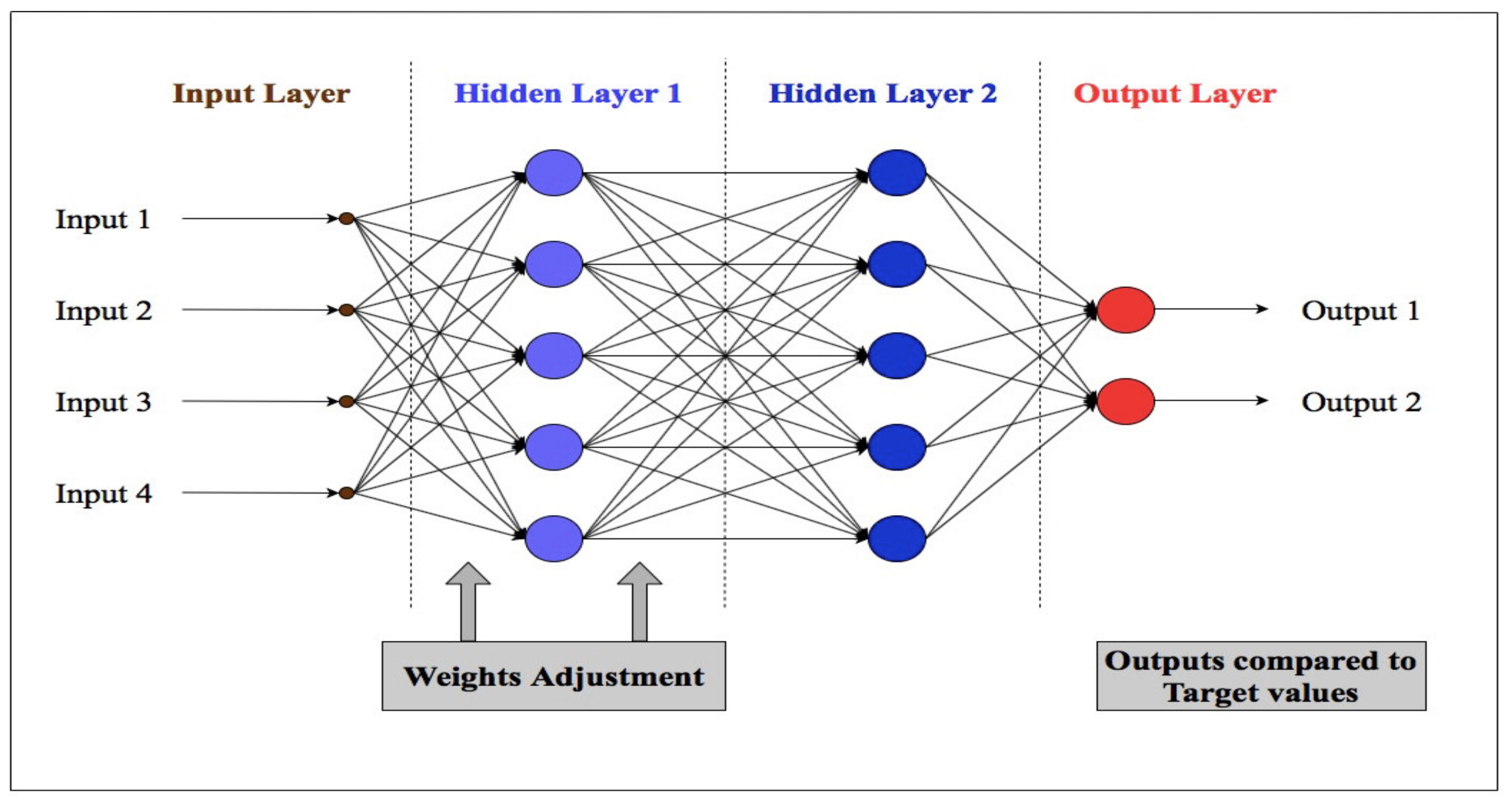
Nitrogen, if present in river water, causes different disorders, which are deleterious for both human and aquatic animals. Nitrogen present in streams are mainly found in three compound states: ammonia, nitrate, and nitrite. Some amounts of ammonia present in the river water get converted to nitrate depending on the dissolved oxygen concentration in the water [43]. As stated earlier, nitrate is not much deleterious, but if present in surplus amount, it starts converting into nitrite, which is very harmful even in minute concentration. The Environmental Protection Agency has set standards which state that for water which is to be distributed for public use, the maximum acceptable nitrate concentration is 10 mg/L [5,25] and that for nitrite is 1 mg/L.
There are two major effects of ammonia on the whole ecosystem: eutrophication of marine and terrestrial ecosystems [44,45] and increase in the acidity of water bodies [46]. Excessive nutrients such as nitrogen and phosphorus when present in water bodies lead to the growth of algae on the top surface of water; this process is termed as eutrophication. Excess grown algae cover the whole water surface, blocking the contact of water from sunlight and air. Additionally, the algae growth decreases the oxygen level in the water body, which affects the aquatic lives. Stream eutrophication was recognized as a major problem years ago, and the United States along with other countries commenced nutrient control measures in rivers [47,48].
Streams may get acidified due to the presence of surfeit ammonia. The most common form of ammonia, ammonium sulphate, leads to formation of a considerable amount of acid, as hydrogen ions are released during nitrification. Additionally, nitrite ions present in the streams lead to the formation of nitric acid under different situations along with sulfate ions, consequently acidifying the stream water [49]. Acidic stream water is not even suitable for reuse to satisfy human water requirements. As stated by Gündüz [50], one day, reuse of treated water would be a reality for the rural population, and this would result in serious problems such as human health issues. Compared with urban areas, agricultural areas are more susceptible to health risks by the presence of nitrate-nitrogen in groundwater [51,52].
Nitrite has been found to be more toxic than nitrate and if present in drinking water can cause human health problems such as liver damage and, in worst cases, can lead to various types of cancer [53] and two types of birth defects [54,55]. Nitrite present in surplus quantity in drinking water will eventually lower the ability of bloodstreams to carry oxygen, leading to the lack of oxygen in the body. Infants and young livestock are lamentably affected, as this causes “blue baby syndrome” [53]. The reaction of nitrites with amines either enzymatically or chemically leads to the formation of potent carcinogenic nitrosamines [53,56].
Consumption of nitrates leads to various tumors in the human body [53,57]. In the digestive system, nitrate leads to the formation of N-nitroso compounds [53,58], which are considered to be carcinogenic. Iodine uptakes can be restricted by nitrates, causing thyroid-related problems [53].

4. ANN

ANN is a black-box computational model [59] that contains interconnected network-like structures passing values to other nodes of the connections. It contains an input layer, hidden layers as required, and an output layer. It is well known for its capability of predicting the non-linear variables [60]. ANN forms the same structure as neurons in the human brain [6,20,61]. It functions like a biological neuron, receiving the input as stimulus, evaluating the stimulus, and then providing the output as the response to the stimulus. Figure 1 represents a simple example of the neural network. The inputs are fed to the nodes in the input layer, and those nodes pass the values of input data to the nodes in hidden layer 1 via interconnecting links. As the values are passed from input nodes to the following nodes, it is multiplied with the weights and then passed to the corresponding layer through a transfer function [62]. Likewise, it is passed up to the output layer, where the error is calculated using target vector. Based on this error, weights get adjusted to obtain the exact weighted combination of the input data for forecasting the target vector.
The major advantage of application of the ANN model, over the traditional model, such as a statistical model, is that it learns itself the complexity of nature, without being explicitly transformed into mathematical form [63,64]. Statistical models have a limitation of assuming additional information to derive a sharp conclusion [65]. The major disadvantage of ANN is that it is susceptible to overfitting. Overfitting is the state in training, beyond which, training error decreases but the model starts losing its ability of generalizing the relation between input and output for the new data set i.e., the testing set data. This results in increasing the testing error and decreasing the overall performance of the model. There are several ways to prevent the model from overfitting, among which a well-known method is early-stopping; in which training process is stopped early. However, if the training is stopped too early then the model fails to learn important information. Hence, training should be stopped accordingly to learn all important information without overfitting.
Many types of ANNs feature different concepts of data processing. Each type is designed differently to obtain a more precise output with less data processing time. This is achieved by changing the network’s architecture. According to Jain et al. [66], based on the network connection pattern, i.e., their architecture, ANN is classified into two categories:
a. Feed-Forward Neural Networks (FFNNs)
FFNN has the simplest network connection pattern in which data flow in the forward direction only, starting from the input layer to hidden layers, and then to the output layer. No loops are formed in the paths of the data flow. As shown in Figure 2, FFNN is classified into three subcomponents: single-layer perceptron, multilayer perceptron, and radial basis function neural network (RBFNN). Single-layer perceptron, which consists of one layer, i.e., the output layer, is the simplest form of neural network. It is mainly used for classifying the linearly separable cases that use binary targets. The connection patterns of multilayer perceptron and RBFNN are the same: an input layer, as many hidden layers as required, and an output layer. The only difference between these two is the use of the data processing function. Multilayer perceptron utilizes either threshold function or sigmoidal function [67] in each of its computational units, whereas RBFNN utilizes radial basis function as the activation function in each unit of its hidden layers. The Table 1 presents the advantages and disadvantages of different models of FFNN. These models are generally used for time series prediction, system control, and data classification.
b. Recurrent or Feedback Neural Networks
Recurrent or feedback neural networks experience the backward flow of data in some computational cells. The data flow is not unidirectional; loops within the cells transfer back the feedback of the errors encountered in computations, with reference to the target values. The feedback of errors helps in updating the weights of the corresponding inputs. As shown in Figure 2, feedback neural network is classified into four subcomponents: adaptive resonance theory model, Hopfield networks, Kohonen’s networks, and competitive networks. Table 1 presents their advantages and disadvantages. These networks form very complex architectures, composed of a number of loops. These networks are utilized for complex computations, such as speech recognition, image processing, robotics, and process controls. This study is limited to the review of the FFNN.

5. Hybrid Model

Hybrid model is the combination of different models to solve a computational task. The need of hybridization aroused when the learning models were observed to be very efficient in some cases and inefficient in most of the cases [68]. The main aim of hybridization is to resolve the limitations of an individual model by fusion of decision making models with learning models [69]. The main advantage of a hybrid model is that it provides better results in comparison to the standalone model. The decision making model integrated in the hybrid model provides a good start with selected initial values of the internal parameters of learning models; hence, increasing the productivity of the learning model. The disadvantages of the hybrid models are: overall training process is time consuming, and complex architecture and training requires modern computational resources. Some of the examples of hybrid models are [70]:
  • ANN and genetic algorithm
  • ANN and fruit fly optimization algorithm
  • ANN and firefly algorithm
  • ANN and artificial immune systems
  • ANN and particle swarm-optimization algorithm

6. Methods and Evaluation

This study is based on nitrogen compounds prediction in water bodies using ANN and other predictive models. In this study, in the section of ‘Application of ANN’, authors have first analyzed the sources of data collection, methods used, internal parameters of the predictive model, and then the final results of the previous research works in literature. On the basis of this analysis, authors have recommended various steps to be followed in future studies for achieving better accuracy models.
As used by [71], authors of this study have used relevant search engines such as Google Scholar and Science Direct. Additionally, the authors of [72] concluded, in their study, that Google Scholar is the most comprehensive source. While searching the relevant literature research works, the following keywords have been used: nitrogen compounds prediction, use of ANN in nitrogen prediction and nitrogen prediction in water bodies.

6.1. Nitrogen Monitoring

More than 60% of the world’s rivers are affected by pollution [43], from point sources or non-point sources. Wastes generated by industrial, municipal, and agricultural activities are discharged into the rivers and pollute them [43,73]. Over time, human activities have escalated nitrogen species concentration in water bodies. Nitrate concentrations in many European rivers have surged by 5- to 10-fold since the 20th century [39]. In Malaysia, because of the excessive chemical pollution in rivers, more than one among the nine water treatment plants in Langat River basin has been closed several times between 2012 and 2015 [41]. According to Selangor Water Management Authority, Malaysia, between 2012 and 2015, the ammonia concentration level in the Langat River exceeded 7.0 mg/L, which led to the repeated closure of many water treatment plants during the period [41]. Moreover, in the Johor River basin, nearly five treatment plants were repeatedly closed between 2017 and 2019 due to the high concentration of ammonia in the Johor River [74,75,76].
There is no specific standard set for ammonia discharge in water bodies, but different agencies have provided separate guidelines for ammonia concentration in water bodies. “Canadian Water Quality Guidelines for the Protection of Aquatic Lives”, [77] states that the guideline value for unionized ammonia discharge in freshwater is a concentration of 0.019 mg/L. The guidelines for drinking water quality (2003) published by WHO states that natural levels of ammonia in groundwater are usually below 0.2 mg/L, and this level may go up to 12 mg/L for surface waters.
For analyzing nitrate variations, Rekacewicz [76] designed a map, as shown in Figure 3, by considering all the river data at continental level, which represent the concentration of nitrate-nitrogen in streams at various locations around the world. Rekacewicz [76] compared the data of two decades and observed that rivers in North America and Europe were fairly stable, but those of south-central Asia and southeast Asia showed high nitrate concentrations.
Furthermore, Basheer et al. [78] studied the water quality of the Langat River in Malaysia. They utilized 10 samples from different locations to quantify different water quality parameters. Their results showed that the pH range for the Langat River was between 5.91 and 6.79. The average value of ammonia for the Langat River was measured to be 0.24 mg/L. The total ammonia-nitrogen amounts added to the Langat River from point and non-point sources were calculated to be 9.51 ton/day and 12.67 ton/day, respectively [41,79], as displayed in Figure 4.
Moreover, Zhang, Swaney, Li, Hong, Howarth and Ding [15] tried to calculate nitrogen input to the Huai River in China from anthropogenic point and non-point sources, and also the impact of nitrogen discharge on the riverine ammonia-nitrogen flux. They used the data from Yan et al. [80], which stated that the average nitrogen concentration in the sewage discharged from industries in the Changjiang River basin was 25 mg/L. From the previous studies, they could conclude that ammonia-nitrogen in the river was about 10% (or less) of the total nitrogen [15,81,82], and it could be as high as 70% in heavily polluted Asian rivers in the urban areas [15,83,84]. They used the data of Zhang et al. [85], which suggested that nitrate had become a major constituent of riverine nitrogen flux; the data was obtained from measurement in 2008, at several stations in the Huai River basin; the values of riverine nitrate concentration was found to vary between 0 and 15.7 mg/L nitrate-nitrogen, with a mean of 2.1 mg/L nitrate-nitrogen. When the authors of [15] measured the ammonia-nitrogen in the same river basin, they found that the average ammonia-nitrogen concentration varied between 0.2 and 3.3 mg/L N, with an average of 1 mg/L N, which was half of the average nitrate-nitrogen concentration measured in 2008. The calculation of nitrogen input to the Huai River showed that on average, 27200 ± 1100 kg km−2y−1 of nitrogen was added to the river from 2003 to 2010 as the net anthropogenic nitrogen input.

6.2. Application of ANN

ANNs have been extensively used worldwide in the past as a predictive model for nitrogen prediction in streams. Table 2 lists studies on the use of ANN by various authors. Various authors had utilized different methodology, as shown in Table 3. For nitrogen prediction, ANN was utilized, for the first time, probably by Lek, Guiresse and Giraudel [20]. They used ANN to predict inorganic and total nitrogen concentration in streams using eight input parameters from the catchments along with the historical data of inorganic and total nitrogen. The input database was obtained from U.S. National Eutrophication Survey (NES); which had many variables in record but according to the scope of the research (prediction of stream nitrogen concentration), the following eight variables were included: average annual flow; animal unit density; mean annual streamflow; the percentages of forest cover, wetland, urban areas, and agriculture areas; and the percentages of the remaining area in the catchment. Sensitivity analysis showed five different types of variation in total nitrogen concentration and three different types of variation in inorganic nitrogen concentration. The sensitivity types (or contribution) for total nitrogen concentration are: (i) Increasing sigmoid contribution: wetland and animal unit density. Low values of these independent variables lead to low (minimum) value of total nitrogen; which then enhances to reach its maximum value with the independent variable. (ii) Weakly growing contribution: agricultural areas. For low values of agricultural areas, the total nitrogen is less and likewise increasing gradually. (iii) Decreasing contribution: average annual flow and percentage of remaining area. (iv) Gaussian: Urban areas. (v) Weak contribution: percentage of forest cover. For inorganic nitrogen: (i) Growing contribution: urban and agricultural areas. For low values of urban and agricultural areas, inorganic nitrogen concentration is less and then rapidly increases with these independent variables. (ii) Gaussian: percentage of wetland areas. (iii) Decreasing contribution: Percentage of forest cover, animal unit density and remaining area. Forest cover rapidly and constantly decreases the inorganic nitrogen concentration. The other two independent variables also reduce the inorganic nitrogen concentration but at low levels only. Input variables were auto-scaled by centered and reduced variables. Autoscaling reduces the chance of domination of any one particular input variable over the prediction. This input database was divided into a training and independent testing set (two thirds and one third of the total database, respectively). Using data from 927 sites from different parts of the United States, Lek, Guiresse and Giraudel [20] developed a multilayer feed-forward ANN model having 10 neurons and 1 hidden layer, with a correlation coefficient of 0.82 for total nitrogen concentration and 0.8 for inorganic nitrogen concentration. Examining the results obtained, they concluded that the urban areas produced most of the inorganic nitrogen, and animal husbandry contributed the most to the total nitrogen concentration in streams. It was assumed that fertilizers were used in less quantities as its contribution was less in stream nitrogen. Forest cover lowered the inorganic nitrogen concentration in streams and has less effect on total nitrogen concentration. Percentage of wetland areas helped in reducing the inorganic nitrogen in streams, but they increased the total nitrogen.
The condition of the United States seemed to be critical in terms of nitrogen in streams, as four years after the study by Lek, Guiresse and Giraudel [20], a research work published by Suen and Eheart [25] stated that nitrate has become an important problem. They conducted a study in the Upper Sangamon River, Illinois, and pointed out the use of chemical fertilizers in agriculture to be responsible for the high nitrate concentration in streams. In their study, they developed two models, RBFNN and backpropagation neural network (BPNN), and compared the models on the basis of accuracy. The parameters used for modeling were daily highest temperature, seven-day cumulative daily rainfall, daily streamflow, and Julian date. To include the common practice of fertilizer application, Julian date was used as an input parameter to the model. They used a dataset of eight years, i.e., 1993–2000. To divide the dataset into the training set and testing set, two methods were adopted. In the first method, data from 1993 to 1996 were used as the training dataset and the remaining were used for testing. For the second method, the data of odd years (i.e., 1993, 1995, 1997, and 1999) were used for training, and those of even years were used for testing. Comparing the results obtained from the models, they concluded that the odd-even years method proved to be more accurate. The overall accuracy of the first method was obtained to be 0.784 and 0.752 for BPNN and RBFNN, respectively, and that of the second method was 0.832 for both the networks. Neural network models predicted with greater precision when tested for Boolean output considering the second method. The network signaled 1 when the nitrate concentration exceeded 10 mg/L and 0 when the nitrate concentration was below 10 mg/L. Considering Boolean output, they concluded that RBFNN had a higher accuracy (0.893) than BPNN (0.866).
In 2003, a research work published in Canada by Sharma, Negi, Rudra and Yang [6] stated that subsurface waters in Canada were being polluted by the nitrate from the fertilizers used in agricultural fields. Their experimental site was a field, of area 14 ha, located at the Greenbelt Research Farm of Agriculture and Agri-Food Canada, near Ottawa. The authors proposed a neural network model to assist in optimizing the use of fertilizers. The input database was collected from the experimental field for the period of 1991–1994, except for the temperature and precipitation data. Data of these two variables were collected at the station of Agriculture and Agri-Food Canada, located 12 km from the site. Two neural network models, fast BPNN and self-organizing RBFNN, were examined, aiming to select the superior network. Inputs to the model used were treatment (tillage or no tillage, i.e., whether the land was prepared or not), Julian day, rainfall per day, cumulative rainfall, total nitrogen applied, snowfall per day, and maximum and minimum temperature. Sensitivity analysis was performed to determine the optimum internal parameters of both the networks. The input data were divided into two sets: training and testing set. Training set consisted of eight input variables and two output, and the testing set consisted of only the unexposed inputs from the replicate plots. For fast BPNN, the parameters varied for sensitivity analysis were learning rate and number of hidden neurons. This analysis comprised of two stages: First stage was to keep the number of hidden neurons constant at 20 and vary the learning rate from 0.02 to 0.08. Analysis of the fluctuation of error on every variation led to the selection of optimum learning rate as 0.02. In the second stage, learning rate was kept constant to 0.02 and number of hidden neurons were varied from 5 to 25. Analyzing the similar way, optimum number of hidden neurons were selected as 20. Similarly, sensitivity analysis was performed for RBFNN, in two stages, by varying the tolerance and spread values from 5 to 20 and 1 to 20, respectively. The selected optimum value for tolerance and spread values were 20 and 15, respectively. Using these parameter values, both the models were further trained. Comparing the results of both networks, the authors concluded that the self-organizing RBFNN, with a correlation coefficient of 0.8079 for conventional tillage and 0.6911 for no tillage, outperformed the fast BPNN, with a correlation coefficient of 0.8017 for conventional tillage and 0.6635 for no tillage, for nitrate-nitrogen concentration prediction in drainage water.
Holmberg, Forsius, Starr and Huttunen [19], predicted the future data of total organic carbon, total nitrogen, and total phosphorus in streams, considering the climate change effect and utilizing the data of three streams (Kelopuro, Hietapuro and Valkea-Kotinen) located in two catchments of the same name (Hietajärvi) in Finland. They developed a BPNN model employing the database of 13 input variables: month of data sampling, mean temperatures of 3 and 10 preceding days, runoff of sampling day, maximum and minimum runoffs of 3 preceding days, days of peak flow, days of low flow, catchment area, fractions of lake area and peatland area with respect to catchment area, catchment latitude, and elevation. This database was collected from the catchment, except for the daily temperature and precipitation, which was collected from the nearby Finnish Meteorological Institute weather station, Lammi, from 1990 to 2000. Samples of these variables were divided into two sets: training set and testing set. The samples were allocated into these sets by random choosing, provided it was ensured that the highest and lowest 10-percentile data were included in both the sets. While training, they were to test all the possible set of models with the available inputs, hence, they varied the number of inputs from 2 to 16, fixing the number of hidden layer to 1 and the neurons in the hidden layer were set as the integer part of (1 + number of inputs)/2. Training 10 sessions for each combination, resultant models were analyzed on the basis of their efficiency. The model resulted the best efficiency with 13 input variables and 1 hidden layer with 7 nodes, having the values of flux efficiencies of total organic carbon, total nitrogen, and total phosphorus as 0.94, 0.92, and 0.90, respectively. Using this model, they forecasted the total nitrogen data until 2050. They stated that if there is a low change in climate, then the total nitrogen flux will be near the value in 2005, but for a scenario of high change in climate, the nitrogen flux will increase by 26%, with respect of the value in 2005.
Similar conditions have been stimulated in Melarchez, a catchment near Paris, France, where Anctil, Filion and Tournebize [61] investigated an agricultural catchment area to develop a neural network model for predicting the nitrate-nitrogen flux. Considering the soil moisture at different depths as the input parameter, the authors analyzed its effect on the nitrate-nitrogen flux. They developed a stacked multilayer perceptron model focusing mainly on the selection of best performing model among the list of models developed, based on different combinations of input variables and neurons in hidden layers. Fifty models were trained for each combination of inputs and neurons in hidden layers. Neurons in hidden layers were varied from 2 to 20. Every issue was tested discretely to make the final decision on the basis of the model accuracy. They had 12 different options for the input parameter: same-day stream flow, previous-day stream flow, increment in the flow from the previous day, same-day precipitation, previous-day precipitation, same-day historical mean flux, increment in the historical mean flux from the previous day, same-day 10 cm-, 20 cm-, 40 cm-, 80 cm-, and 120 cm-depth soil moisture indices. These input variables were collected from the gauge station for the period of 1975 to 1993. Since the important step, in pre-processing of data, is standardization [91], all the input variables were ensured to be on the same scale by standardizing them linearly such that their standard deviation as 1 and mean as 0. After optimizing, the final model had 2 input parameters (same-day stream flow and same-day 80 cm-depth soil moisture index), 12 neurons in hidden layers, and Levenberg-Marquardt with Bayesian regulation as the calibration procedure, which performed well with an efficiency index of 0.888. The utilization of soil moisture content at different depths revealed that the soil moisture also had an effect on nitrate-nitrogen flux generated from the agricultural field.
Since a large number of input variables are available to decide for the neural network, these inputs should be chosen using sensitivity analysis [92]. Numerous authors have provided models with different sets of input parameters, which according to them, were suitable for their models (Table 4). He, Oki, Sun, Komori, Kanae, Wang, Kim and Yamazaki [18] investigated 59 river basins all over Japan and developed an FFNN to predict the monthly total nitrogen concentrations in streams. They had to choose the most important independent input variables from a set of 16 input variables: the area of each basin, amount of fertilizer applied in each basin, average temperature, precipitation, sunshine duration and river discharge of each basin, ratio of paddy area, farmland area, forest area, bare land area, urban area, road area, river area, lake area, seashore area, and other land areas in the total basin area. This input database was collected from different sources. The land use variables were collected from Ministry of Land, Infrastructure, Transport and Tourism (MLIT land use database), a digital database in Japan. Total nitrogen concentration was collected from MLIT water information system. Sunshine duration, precipitation and temperature data were obtained from Automated Meteorological Data Acquisition System. The input data were divided into three subsets: Training, overfitting test and validation subsets. Among the data of 59 river basins, 40 river basin data were used for training and overfitting test (80% and 20%, respectively). The remaining 19 river basin data were never exposed to the network for training and were used for validation only. FFNN was trained with backpropagation algorithm with different combinations of input variables and internal parameters: input variables were varied from 7 to 9, number of hidden layers was fixed to 1 with number of neurons in it fixed to 7 and 8. Analyzing the results of all the trained network on the basis of coefficient of regression, the authors found that the model with 8 input variables (river discharge, average temperature and precipitation of each basin, amount of fertilizer applied in each basin, the proportions of forest land area, urban land area, road area, and other areas in the total basin area) and one hidden layer with seven nodes provided the best accuracy with R2 for training as 0.96, R2 for validation as 0.84, and R2 for overfitting as 0.90.
In addition to ANN, other machine learning methods can also be used to predict nonlinear environmental variables. Wang, Oldham and Hipsey [86] compared 13 machine learning models, including ANN, on the basis of precision in the prediction of DON (dissolved organic nitrogen) in groundwater in urban areas in southwestern Australia. These 13 machine learning models are classified into five different groups: (1) tree-based and rule-based model (generalized busted model (GBM), RF (Random Forest), conditional inference random forest (cforest), and cubist); (2) kernel-based machine learning model (Gaussian process with radial basis function kernel (GPR), Gaussian process with linear kernel (GPL), support vector machine with radial basis function kernel (SVMR), and support vector machine with linear kernel (SVML)); (3) generalized stepwise linear regression models (bagged mars, multivariate adaptive regression spline (mars), and generalized linear model with stepwise feature selection (GLM)); (4) instance-based model (k-nearest neighbors (KNNs)); and (5) ANNs. Using 401 groundwater samples (60% for training and 40% for testing), the models were examined based on two scenarios: (1) to train the models with all the data available such as nutrients (DON, total nitrogen, N H 4 + , and N O x ), landscape (vegetation, land use, and soil), hydrological conditions (surface water subarea, groundwater subarea, and catchment area), and sampling conditions (temperature, sample depth, sampling date, and pH); (2) to train the models with only total nitrogen and all other non-nutrient data. Database of nutrients were obtained from the Western Australian Department of Water for the period of 2006-2014. ArcGIS spatial mapping feature provided the data of soil type, land use and vegetation type. These models were analyzed on the basis of their RMSE and R2 values and compared with the manually calculated DON (DONcal) (Figure 5). Analysis of all the results revealed that scenario 1 produced lower errors in models than scenario 2, stating that nutrients can improve the performance of models. Among the 13 tested models, 3 models showed higher R2 value. For scenarios 1 and 2, the cubist model had R2 values of 0.897 and 0.849; bagged mars, 0.882 and 0.887; random forest, 0.856 and 0.858; and ANN, about 0.72 and 0.65, respectively.
Zhang, Zhang and Li [87] compared ARIMA model, RBFNN model, and hybrid ARIMA-RBFNN model based on the analysis and prediction of water quality in Chagan Lake, China. Database of water quality was collected from “The Second Songhua River Diversion Project Record” from the Chinese Academy of Science. The water quality parameters utilized for analysis were monthly total nitrogen and total phosphorus for the period of 2006–2011. The parameters of ARIMA model for total nitrogen were p = 1, d = 1 and q = 1 and for total phosphorus were p = 2, d = 1 and q = 1. Water quality data from 2006 to 2010 were used for training and the trained model was used for prediction of water quality data of 2011. The width of training, σ, was 0.6 for RBFNN model with 2 nodes in hidden layers. ARIMA-predicted values were linearly super-positioned with RBFNN-derived ARIMA residual prediction values to generate the hybrid ARIMA-RBFNN model. These models were analyzed on the basis of their RMSE and mean absolute percentage error. Results showed that RBFNN model had bad prediction results for total phosphorus; though, this model had learned the pattern of total nitrogen, but the predicted values were not satisfactory. Although ARIMA model did not have high prediction accuracy, it had successfully learned various trends for both total nitrogen and total phosphorus. Analyzing the results obtained, the mean absolute percentage error for the monthly total nitrogen was 18,194%, 34,633%, and 7017% for ARIMA, RBFNN, and hybrid ARIMA-RBFNN, respectively, and the mean absolute percentage error for the monthly total phosphorus was 27,299%, 126,957%, and 14,528% for ARIMA, RBFNN, and hybrid ARIMA-RBFNN, respectively. Following the results, it was stated that hybrid models had more capacity in predicting nonlinear variables.
Markus, Hejazi, Bajcsy, Giustolisi and Savic [88] developed three models—BPNN, EPR and NBM—for predicting weekly nitrate-nitrogen in a small agricultural watershed in Illinois. For the ANN part, the authors utilized observed weekly river discharge, precipitation, air temperature, and nitrate-nitrogen concentration as input variables. The study used the historical data of nitrate-nitrogen concentration and was collected from the Upper Sangamon River near Decatur for the period of 1994-1999. Employing half of the data for training and the other half for testing, they predicted the weekly data of nitrate-nitrogen in streams. The input selection was performed on the basis of trial and error with two sets of variables and their time lags. The first set consisted of four variables: N t ,   Q t ,   T t ,   P t ; and the second set consisted of four variables and three time lags N t ,   Q t ,   T t ,   P t ,   Q t 1 ,   T t 1 ,   P t 1 . The first set predicted better results and hence was used for ANN modeling. ERP model has the capability of selecting the input subset, hence it is fed with the larger input set, the second set. In case of NBM, both the sets were used for modeling. For modeling in the ANN part, the internal parameters selected were: epochs: 100,000; performance gradient: 1E-10; goal: 0; number of hidden nodes: 1, 2, 3, 4 and 5; input variables: 4 (air temperature, discharge, nitrate-N concentration and precipitation) and output variable: 1 (next week nitrate-N concentration). The results indicated that the ANN with 2 nodes showed more accurate results in terms of RMSE as 0.787 mg/L and 0.935 mg/L for training and testing, respectively. For EPR, two models (EPR1 and EPR2) were generated which had their equations as: N t + 1 = 0.827 N t and N t + 1 = 0.659 N t + 0.560 N t Q t , respectively. The RMSE obtained for EPR1 was 1.092 mg/L for training and 1.170 mg/L for testing. The RMSE obtained for the EPR2 was more accurate: 0.991 mg/L and 1.010 mg/L for training and testing, respectively. The NBM model utilized two categories: high and low values for variables. Each variable, except for nitrate-N concentration, had its categories divided by the average values as threshold. For nitrate-N concentration, the separation point was the emergency cutoff level (8.5 mg/L). NBM1 and NBM2 were the two models tested with the equations as: N t + 1 = f N t ,   Q t ,   P t ,   T t and N t + 1 = f N t ,   Q t ,   Q t 1 ,   P t ,   P t 1 ,   T t ,   T t 1 , respectively. The results of these models indicated that, for low concentration, NBM1 had accurately predicted 79 of 80 concentrations, but for high concentrations, the prediction rate was 2 of 9. For NBM2, the predicted high flows (10) were somewhat similar to the observed ones (9). However, the false alarm rate for NBM2 was higher (7) than NBM1 (1). The critical success index for NBM1 was obtained as 0.214 and 0.200 for training and testing, respectively, and that for NBM2 was 0.286 and 0.188 for training and testing, respectively. The authors concluded that none of these models can be considered superior based on this analysis criteria, hence, suggesting a multi-tool approach. In their previous study, Markus et al. [93] compared the ANN model and linear regression model to calculate the uncertainty in forecasting the weekly nitrate-nitrogen in the Sangamon River, Illinois. They stated that the ANN model was more accurate than the linear regression model. The ANN model surpassed the linear regression model by 3.30% and 4.42% of RMSE in testing and training phases, respectively.
Amiri and Nakane [89] compared BPNN and MLR on the basis of the total nitrogen prediction in streams. The study was conducted in the Chugoku district of Japan, which contains 21 river basins. Total nitrogen database, for year 2001, was collected from prefecture offices from Okayama, Shimane, Hiroshima, Tottori and Yamaguchi. Six input variables were used for the prediction, which included five variables for land cover percentage (urban area, forest area, agriculture area, grassland, and water body) and the last variable for population density. The total nitrogen was predicted by utilizing 60% of the data for training, 25% for controlling, and the remaining 15% for testing. BPNN consisted of six input nodes for the corresponding six input variables, one hidden layer and one node in output layer for total nitrogen prediction. The optimum number of nodes in hidden layer were selected by varying the nodes from 0 to 13 and training the network 5 times for each variation and evaluating them on the basis of correlation coefficient. The selected optimum BPNN had the following internal parameters: input nodes: 6, hidden layer: 1, hidden layer node: 2, output node: 1, epochs: 11, 600. MLR model had the same inputs as for the BPNN. For MLR modeling, a normality test was conducted for total nitrogen and land cover data using Sharpio-Wilk test having p-value less than 0.05. Models were analyzed on the basis of regression statistics and coefficient of the model (if the resultant was normally distributed). Final regression model was developed by using backward approach. The goodness of fit of the models was evaluated by regression of observed versus predicted and scatter plot. Comparison of the results for both the models showed that the backpropagation model (R2 = 0.94) predicted the results more precisely than the multiple regression model (R2 = 0.85)
Zeleňáková, Čarnogurská, Šlezingr and Słyś [90] predicted nitrogen and phosphorus concentrations in river Laborec in Slovakia, employing dimensional analysis method. They used Buckingham theorem to develop a prediction model utilizing important variables such as stream discharge, area of catchment, stream velocity, temperatures of air and water, and pollutant concentration. The equation established for nitrogen concentration was: π 1 = 0.0039 π 2 13.805 and for phosphorus was: π 1 = 0.1868 π 2 9.7892 . These models were tested for the data of eight years (2003–2010); which was collected from Slovak Hydrometeorological Institute and Slovakian Water Management Company in Košice. Sensitivity analysis of the model stated that air and water temperature have major influence on the prediction of concentration of nitrogen and phosphorus. Velocity and flow of water have less influence and the catchment area has no influence on the prediction. By exploring the results of the model, it was found that the model equations calculated the prediction values with an average uncertainty of 31.33% for nitrogen and 32.30% for phosphorus.

7. Recommendation for Future Works

The precision of the predictive ANN model relies on many factors such as the amount of input data provided to the model for training and testing, relevant input variables, and different types of ANN methods used in the model. Based on the reviewed research works, we suggest some techniques to improve the accuracy of the nitrogen predicting model and also to account for a large range of inputs.
a)
Being the first step of modeling, the training is the most important part of the modeling procedure. Various kinds of important information are provided to the model during training. The model learns different patterns in the input data. Weights are updated during training [94]. Providing ample data for training can lead to better precision of the model. Input data is divided into three sets: training, testing and validation sets [95], and sometimes divided into two sets: training and testing set, depending on the model. Training set is used for updating the weights and biases of the model. Validation set is used for preventing the model from overfitting. While training, if the validation accuracy is decreasing, then the model seems to be overfitting and the training should be stopped. Testing set is used for testing the output of the model in order to confirm the accuracy of the model. These sets are divided on certain percentage of input data, either provided by user or divided, by default, by the model. By default, ANN modeling software uses 70% of the input data as the training data, which may be less for getting higher accuracy, 15% for validation and the remaining 15% for testing. In order to increase the accuracy of the model, we suggest using a higher percentage of data for training, i.e., about 80% to 90%. The remaining is to be divided equally for validation and testing. While dividing the input data into the training, validation and testing set, it should be ensured that these sets are statistically similar. In order to increase the learning capacity of the model, it should be ensured that the model is exposed to the maximum and minimum values of the inputs while training.
b)
The accuracy of the AI model also depends on the types of inputs provided to the model [96]. Since there are many input variables upon which the nitrogen in streams depends, we suggest considering all the relevant inputs and then performing a sensitivity analysis to select the highly sensitive input variables for the prediction. Some of the relevant inputs are daily average rainfall data, daily average river discharge, daily average water temperature, historical data of nitrogen in streams, land use pattern, Julian day, amount of fertilizer applied in the catchment area, and the amount of nitrogen per day added from point sources. Using many input variables leads to the increase in the complexity of the network, which often effects the results of the network. To avoid this complexity, the user should avoid selecting the inter-dependent variables, for example: if the runoff data is included in the input data then the precipitation data can be avoided because runoff is dependent on precipitation and has the same pattern as that of precipitation.
c)
ANN is divided into different types, which are utilized for modeling hydrological parameters having different complexity levels. For creating a model involving a huge set of input variables, we suggest creating a hybrid model, which has higher accuracy. The ANN model has to be clipped with other models to create a hybrid model, and hence, it improves the accuracy of the resultant model. Zhang, Zhang and Li [87] utilized a hybrid model (ARIMA and RBFNN) to predict the monthly total nitrogen, and the mean absolute percentage error was reduced to 7.017%. However, in this case, they used only historical monthly data as input to the hybrid model; hence, a hybrid model with a wide range of relevant stochastic input variables will attain increased accuracy.

8. Conclusions

This research paper reviews the previous uses of ANN for the prediction of nitrogen compounds in streams. The efforts that have been made in past decades to predict the nitrogen compounds with greater accuracy are also demonstrated in this work. The current condition of rivers in terms of nitrogen compound concentration is discussed. The major non-point source of nitrogen in the streams is the fertilizer applied in agricultural fields. Excess nitrogen concentration in streams leads to human health issues. The operations of many water treatment plants depend on the concentration of nitrogen in the river. In the past two decades, ANNs have shown greater reliability in predicting the nitrogen compounds and have also helped in optimizing the sources of nitrogen input to the streams. The analysis of the literature reveals that published papers on the prediction of nitrogen compounds using hybrid models are limited. This study suggests the usage of a hybrid model along with the set of suggested relevant input variables and training procedures.

Author Contributions

Conceptualization, A.E.-S. and H.A.A.; Methodology, P.K. and A.E.-S.; Formal Analysis, S.H.L.; Investigation, P.K.; Resources, A.E.-S.; Data Curation, S.H.L.; Writing—Original Draft Preparation, P.K.; Writing—Review & Editing, J.K.W., M.S., and A.S.; Visualization, M.S., A.S., and A.N.A.; Supervision, A.E.-S., S.H.L., N.S.M. and M.R.K.; Project Administration, A.E.-S.; Funding Acquisition, A.E.-S. All authors have read and agreed to the published version of the manuscript.

Funding

This research was funded by University of Malaya Research Grant (UMRG), grant number RP025A-18SUS.

Acknowledgments

The authors appreciate so much the facilities support by the Civil Engineering Department, Faculty of Engineering, University of Malaya, Malaysia.

Conflicts of Interest

We declare no conflicts of interest with any person or institute.

References

  1. Maloney, K.O.; Weller, D.E. Anthropogenic disturbance and streams: Land use and land-use change affect stream ecosystems via multiple pathways. Freshw. Biol. 2011, 56, 611–626. [Google Scholar] [CrossRef]
  2. Kilonzo, F.; Masese, F.O.; Van Griensven, A.; Bauwens, W.; Obando, J.; Lens, P.N.L. Spatial–temporal variability in water quality and macro-invertebrate assemblages in the Upper Mara River basin, Kenya. Phys. Chem. EarthParts A/B/C 2014, 67–69, 93–104. [Google Scholar] [CrossRef]
  3. Jacobs, S.R.; Breuer, L.; Butterbach-Bahl, K.; Pelster, D.E.; Rufino, M.C. Land use affects total dissolved nitrogen and nitrate concentrations in tropical montane streams in Kenya. Sci. Total Env. 2017, 603–604, 519–532. [Google Scholar] [CrossRef] [PubMed]
  4. Hessong, A. The Composition of Fertilizers. Available online: http://homeguides.sfgate.com/composition-fertilizers-48898.html (accessed on 26 June 2019).
  5. Salehi, F.; Prasher, S.O.; Amin, S.; Madani, A.; Jebelli, S.J.; Ramaswamy, H.S.; Tan, C.; Drury, C.F. Prediction of annual nitrate-n losses in drain outflows with artificial neural networks. Am. Soc. Agric. Eng. 2000, 43, 1137–1143. [Google Scholar] [CrossRef]
  6. Sharma, V.; Negi, S.C.; Rudra, R.P.; Yang, S. Neural networks for predicting nitrate-nitrogen in drainage water. Agric. Water Manag. 2003, 63, 169–183. [Google Scholar] [CrossRef]
  7. Fewtrell, L. Drinking-water nitrate, methemoglobinemia, and global burden of disease: A discussion. Environ. Health Perspect 2004, 112, 1371–1374. [Google Scholar] [CrossRef] [Green Version]
  8. Gallo, E.L.; Meixner, T.; Aoubid, H.; Lohse, K.A.; Brooks, P.D. Combined impact of catchment size, land cover, and precipitation on streamflow and total dissolved nitrogen: A global comparative analysis. Glob. Biogeochem. Cycles 2015, 29, 1109–1121. [Google Scholar] [CrossRef]
  9. Ward, M.H.; deKok, T.M.; Levallois, P.; Brender, J.; Gulis, G.; Nolan, B.T.; VanDerslice, J.; International Society for Environmental. Workgroup report: Drinking-water nitrate and health--recent findings and research needs. Environ. Health Perspect 2005, 113, 1607–1614. [Google Scholar] [CrossRef] [Green Version]
  10. Reddy, A.G.S.; Niranjan Kumar, K.; Subba Rao, D.; Sambashiva Rao, S. Assessment of nitrate contamination due to groundwater pollution in north eastern part of Anantapur District, A.P. India. Environ. Monit. Assess. 2009, 148, 463–476. [Google Scholar] [CrossRef]
  11. Hamed, Y.; Awad, S.; Ben Sâad, A. Nitrate contamination in groundwater in the Sidi Aïch–Gafsa oases region, Southern Tunisia. Environ. Earth Sci. 2013, 70, 2335–2348. [Google Scholar] [CrossRef]
  12. Rahmati, O.; Samani, A.N.; Mahmoodi, N.; Mahdavi, M. Assessment of the Contribution of N-Fertilizers to Nitrate Pollution of Groundwater in Western Iran (Case Study: Ghorveh–Dehgelan Aquifer). Water Qual. Expo. Health 2015, 7, 143–151. [Google Scholar] [CrossRef]
  13. Räike, A.; Pietiläinen, O.P.; Rekolainen, S.; Kauppila, P.; Pitkänen, H.; Niemi, J.; Raateland, A.; Vuorenmaa, J. Trends of phosphorus, nitrogen and chlorophyll a concentrations in Finnish rivers and lakes in 1975–2000. Sci. Total Environ. 2003, 310, 47–59. [Google Scholar] [CrossRef]
  14. Qiu, Y.; Shi, H.-C.; He, M. Nitrogen and Phosphorous Removal in Municipal Wastewater Treatment Plants in China: A Review. Int. J. Chem. Eng. 2010, 2010, 1–10. [Google Scholar] [CrossRef] [Green Version]
  15. Zhang, W.S.; Swaney, D.P.; Li, X.Y.; Hong, B.; Howarth, R.W.; Ding, S.H. Anthropogenic point-source and non-point-source nitrogen inputs into Huai River basin and their impacts on riverine ammonia–nitrogen flux. Biogeosciences 2015, 12, 4275–4289. [Google Scholar] [CrossRef] [Green Version]
  16. Indah Water, M. Ammonia. Available online: https://www.iwk.com.my/do-you-know/ammonia (accessed on 6 July 2019).
  17. Fogelman, S.; Blumenstein, M.; Zhao, H. Estimation of chemical oxygen demand by ultraviolet spectroscopic profiling and artificial neural networks. Neural Comput. Appl. 2005, 15, 197–203. [Google Scholar] [CrossRef]
  18. He, B.; Oki, T.; Sun, F.; Komori, D.; Kanae, S.; Wang, Y.; Kim, H.; Yamazaki, D. Estimating monthly total nitrogen concentration in streams by using artificial neural network. J. Env. Manag. 2011, 92, 172–177. [Google Scholar] [CrossRef]
  19. Holmberg, M.; Forsius, M.; Starr, M.; Huttunen, M. An application of artificial neural networks to carbon, nitrogen and phosphorus concentrations in three boreal streams and impacts of climate change. Ecol. Model. 2006, 195, 51–60. [Google Scholar] [CrossRef]
  20. Lek, S.; Guiresse, M.; Giraudel, J.-L. Predicting stream nitrogen concentration from watershed features using neural networks. Water Resour. Res. 1999, 33, 3469–3478. [Google Scholar] [CrossRef] [Green Version]
  21. Sarangi, A.; Bhattacharya, A.K. Comparison of Artificial Neural Network and regression models for sediment loss prediction from Banha watershed in India. Agric. Water Manag. 2005, 78, 195–208. [Google Scholar] [CrossRef]
  22. Ehtram, M.; Karami, H.; Mousavi, S.-F.; El-Shafie, A.; Amini, Z. Optimizing Dam and Reservoirs Operation Based Model Utilizing Shark Algorithm Approach. Knowl. -Based Syst. 2017. [Google Scholar] [CrossRef]
  23. Aguilera, P.A.; Frenich, A.G.; Torres, J.A.; Castro, H.; Vidal, J.L.M.; Canton, M. Application of the kohonen neural network in coastal water management: Methodological development for the assessment and prediction of water quality. Water Resources 2001, 35, 4053–4062. [Google Scholar] [CrossRef]
  24. Chang, L.-C.; Chang, F.-J. Intelligent control for modelling of real-time reservoir operation. Hydrol. Process. 2001, 15, 1621–1634. [Google Scholar] [CrossRef]
  25. Suen, J.-P.; Eheart, J.W. Evaluation of Neural Networks for Modeling Nitrate Concentrations in Rivers. J. Water Resour. Plan. Manag. ASCE 2003, 129, 505–510. [Google Scholar] [CrossRef]
  26. Zaheer, I.; Bai, C.-G. Application of artificial neural network for water quality management. Lowl. Technol. Int. 2003, 5, 10–15. [Google Scholar]
  27. Tayfur, G.; Swiatek, D.; Wita, A.; Singh, V.P. Case Study: Finite Element Method and Artificial Neural Network Models for Flow through Jeziorsko Earthfill Dam in Poland. J. Hydraul. Eng. 2005, 131, 431–440. [Google Scholar] [CrossRef]
  28. Mazvimavi, D.; Meijerink, A.M.J.; Savenije, H.H.G.; Stein, A. Prediction of flow characteristics using multiple regression and neural networks: A case study in Zimbabwe. Phys. Chem. EarthParts A/B/C 2005, 30, 639–647. [Google Scholar] [CrossRef]
  29. He, B.; Takase, K. Application of the Artificial Neural Network Method to Estimate the Missing Hydrologic Data. J. Jpn. Soc. Hydrol. Water Resour. 2006, 19, 249–257. [Google Scholar] [CrossRef] [Green Version]
  30. Cigizoglu, H.K.; Alp, M. Rainfall-Runoff Modelling Using Three Neural Network Methods. ICAISC 2004, 166–171. [Google Scholar]
  31. Riad, S.; Mania, J.; Bouchaou, L.; Najjar, Y. Rainfall-runoff model usingan artificial neural network approach. Math. Comput. Model. 2004, 40, 839–846. [Google Scholar] [CrossRef]
  32. Shamseldin, A.Y.; Nasr, A.E.; O’Connor, K.M. Comparison of different forms of the Multi-layer Feed-Forward Neural Network method used for river flow forecasting. Hydrol. Earth Syst. Sci. Discuss. 2002, 6, 671–684. [Google Scholar] [CrossRef]
  33. Teschl, R.; Randeu, W.L. A neural network model for short term river flow prediction. Nat. Hazards Earth Syst. Sci. 2006, 6, 629–635. [Google Scholar] [CrossRef] [Green Version]
  34. Wu, C.L.; Chau, K.W. Rainfall–runoff modeling using artificial neural network coupled with singular spectrum analysis. J. Hydrol. 2011, 399, 394–409. [Google Scholar] [CrossRef] [Green Version]
  35. Gazzaz, N.M.; Yusoff, M.K.; Aris, A.Z.; Juahir, H.; Ramli, M.F. Artificial neural network modeling of the water quality index for Kinta River (Malaysia) using water quality variables as predictors. Mar. Pollut Bull. 2012, 64, 2409–2420. [Google Scholar] [CrossRef] [PubMed]
  36. Khalil, B.; Ouarda, T.B.M.J.; St-Hilaire, A. Estimation of water quality characteristics at ungauged sites using artificial neural networks and canonical correlation analysis. J. Hydrol. 2011, 405, 277–287. [Google Scholar] [CrossRef]
  37. Palani, S.; Liong, S.Y.; Tkalich, P. An ANN application for water quality forecasting. Mar. Pollut Bull. 2008, 56, 1586–1597. [Google Scholar] [CrossRef]
  38. Singh, K.P.; Basant, A.; Malik, A.; Jain, G. Artificial neural network modeling of the river water quality—A case study. Ecol. Model. 2009, 220, 888–895. [Google Scholar] [CrossRef]
  39. Suo, W.Q.; Dong-Bao, S.; Wei-Ping, H.; Yu-Zhong, L.; Xu-Rong, M.; Yan-Qing, Z. Human activities and nitrogen in waters. Acta Ecol. Sin. 2012, 32, 174–179. [Google Scholar] [CrossRef]
  40. USGS. Nitrogen and Water. Available online: https://www.usgs.gov/special-topic/water-science-school/science/nitrogen-and-water?qt-science_center_objects=0#qt-science_center_objects (accessed on 26 June 2019).
  41. Farid, A.M.; Lubna, A.; Choo, T.G.; Rahim, M.C.; Mazlin, M. A Review on the Chemical Pollution of Langat River, Malaysia. Asian J. Water Environ. Pollut. 2016, 13, 9–15. [Google Scholar] [CrossRef]
  42. Yi, Q.; Chen, Q.; Hu, L.; Shi, W. Tracking nitrogen sources, transformation and transport at a basin scale with complex plain river networks. Environ. Sci. Technol. 2017. [Google Scholar] [CrossRef]
  43. Nuruzzaman, M.; Mamun, A.A.; Salleh, M.N.B. Determining ammonia nitrogen decay rate of Malaysian river water in a laboratory flume. Int. J. Environ. Sci. Technol. 2017, 15, 1249–1256. [Google Scholar] [CrossRef] [Green Version]
  44. Rabalais, N.N.; Turner, R.E.; Scavia, D. Beyond Science into Policy: Gulf of Mexico Hypoxia and the Mississippi River. Bioscience 2002, 52, 129–142. [Google Scholar] [CrossRef] [Green Version]
  45. Rabalais, N.N.; Turner, R.E. Oxygen depletion in the gulf of mexico adjacent to the mississippi river. Past Present Water Column Anoxia 2006, 225–245. [Google Scholar]
  46. Hessen, D.O.; Hindar, A.; Holtan, G. The Significance of Nitrogen Runoff for Eutrophication of Freshwater and Marine Recipients. R. Swed. Acad. Sci. 1997, 26, 312–320. [Google Scholar]
  47. Dodds, W.; Smith, V. Nitrogen, phosphorus, and eutrophication in streams. Inland Waters 2016, 6, 155–164. [Google Scholar] [CrossRef]
  48. Dodds, W.K.K.; Welch, E.B. Establishing nutrient criteria in streams. J. N. Am. Benthol. Soc. 2000, 19, 186–196. [Google Scholar] [CrossRef]
  49. Murdoch, P.S.; Stoddard, J.L. The Role of Nitrate in the Acidification of Streams in the Catskill Mountains of New York. Water Resour. Res. 1992, 28, 2707–2720. [Google Scholar] [CrossRef]
  50. Gündüz, O. Water Quality Perspectives in a Changing World. Water Qual. Expo. Health 2015, 7, 1–3. [Google Scholar] [CrossRef] [Green Version]
  51. Su, X.; Wang, H.; Zhang, Y. Health Risk Assessment of Nitrate Contamination in Groundwater: A Case Study of an Agricultural Area in Northeast China. Water Resour. Manag. 2013, 27, 3025–3034. [Google Scholar] [CrossRef]
  52. He, S.; Wu, J. Hydrogeochemical Characteristics, Groundwater Quality, and Health Risks from Hexavalent Chromium and Nitrate in Groundwater of Huanhe Formation in Wuqi County, Northwest China. Expo. Health 2019, 11, 125–137. [Google Scholar] [CrossRef]
  53. Hossain, F.; Chang, N.-B.; Wanielista, M.; Xuan, Z.; Daranpob, A. Nitrification and Denitrification in a Passive On-site Wastewater Treatment System with a Recirculation Filtration Tank. Water Qual. Expo. Health 2010, 2, 31–46. [Google Scholar] [CrossRef]
  54. Gulis, G.; Czompolyova, M.; R Cerhan, J. An Ecologic Study of Nitrate in Municipal Drinking Water and Cancer Incidence in Trnava District, Slovakia. Environ. Res. 2002, 88, 182–187. [Google Scholar] [CrossRef] [PubMed]
  55. Chen, J.; Wu, H.; Qian, H.; Gao, Y. Assessing Nitrate and Fluoride Contaminants in Drinking Water and Their Health Risk of Rural Residents Living in a Semiarid Region of Northwest China. Expo. Health 2017, 9, 183–195. [Google Scholar] [CrossRef]
  56. Sawyer, C.N.; McCarty, P.L.; Parkin, G.F. Chemistry for Environmental Engineering and Science, 5th ed.; McGraw Hill: New York, NY, USA, 2003; p. 667. [Google Scholar]
  57. Aslan, S.; Turkman, A. Biological denitrification of drinking water using various natural organic solid substrates. Water Sci. Technol. A J. Int. Assoc. Water Pollut. Res. 2003, 48, 489–495. [Google Scholar] [CrossRef]
  58. Della Rocca, C.; Belgiorno, V.; Meric, S. Cotton-supported heterotrophic denitrification of nitrate-rich drinking water with a sand filtration post-treatment. Water SA 2005, 31, 229–236. [Google Scholar] [CrossRef] [Green Version]
  59. Akrami, S.A.; El-Shafie, A.; Jaafar, O. Improving Rainfall Forecasting Efficiency Using Modified Adaptive Neuro-Fuzzy Inference System (MANFIS). Water Resour Manag. 2013. [Google Scholar] [CrossRef]
  60. Farzad, F.; El-Shafie, A.H. Performance Enhancement of Rainfall Pattern – Water Level Prediction Model Utilizing Self-Organizing-Map Clustering Method. Water Resour Manag. 2016. [Google Scholar] [CrossRef]
  61. Anctil, F.; Filion, M.; Tournebize, J. A neural network experiment on the simulation of daily nitrate-nitrogen and suspended sediment fluxes from a small agricultural catchment. Ecol. Model. 2009, 220, 879–887. [Google Scholar] [CrossRef] [Green Version]
  62. El-Shafie, A.H.; El-Shafie, A.; Mazoghi, H.G.E.; Shehata, A.; Taha, M.R. Artificial neural network technique for rainfall forecasting applied to Alexandria, Egypt. Int. J. Phys. Sci. 2011, 6, 1306–1316. [Google Scholar] [CrossRef]
  63. Raju, M.M.; Srivastava, R.K.; Bisht, D.C.S.; Sharma, H.C.; Kumar, A. Development of Artificial Neural-Network-Based Models for the Simulation of Spring Discharge. Adv. Artif. Intell. 2011, 2011, 1–11. [Google Scholar] [CrossRef] [Green Version]
  64. Shafie, A.H.E.; El-Shafie, A.; Almukhtar, A.; Taha, M.R.; Mazoghi, H.G.E.; Shehata, A. Radial basis function neural networks for reliably forecasting rainfall. J. Water Clim. Chang. 2012. [Google Scholar] [CrossRef]
  65. Xie, Y. Values and Limitations of Statistical Models. Res. Soc. Strat. Mobil 2011, 29, 343–349. [Google Scholar] [CrossRef] [PubMed] [Green Version]
  66. Jain, A.K.; Mao, J.; Mohiuddin, K.M. Artificial Neural Networks: A Tutorial. IEEE 1996, 31–44. [Google Scholar] [CrossRef] [Green Version]
  67. El-Shafie, A.; Noureldin, A.; Taha, M.; Hussain, A.; Mukhlisin, M. Dynamic versus static neural network model for rainfall forecasting at Klang River Basin, Malaysia. Hydrol. Earth Syst. Sci. 2012, 1151–1169. [Google Scholar] [CrossRef] [Green Version]
  68. Voyant, C.; Muselli, M.; Paoli, C.; Nivet, M.-L. Numerical weather prediction (NWP) and hybrid ARMA/ANN model to predict global radiation. Energy 2012, 341–355. [Google Scholar] [CrossRef] [Green Version]
  69. Grosan, C.; Abraham, A. Intelligent Systems A Modern Approach; Springer: Berlin/Heidelberg, Germany, 2011; Volume 17. [Google Scholar]
  70. Fallah, S.N.; Deo, R.C.; Shojafar, M.; Conti, M.; Shamshirband, S. Computational Intelligence Approaches for Energy Load Forecasting in Smart Energy Management Grids: State of the Art, Future Challenges, and Research Directions. Energies 2018, 11, 596. [Google Scholar] [CrossRef] [Green Version]
  71. Fiyadh, S.S.; AlSaadi, M.A.; Jaafar, W.Z.; AlOmar, M.K.; Fayaed, S.S.; Mohd, N.S.; Hin, L.S.; El-Shafie, A. Review on heavy metal adsorption processes by carbon nanotubes. J. Clean. Prod. 2019, 783–793. [Google Scholar] [CrossRef]
  72. Martín-Martín, A.; Thelwall, M.; Orduna-Malea, E.; López-Cózar, E.D. Google Scholar, Microsoft Academic, Scopus, Dimensions, Web of Science, and OpenCitations’ COCI: A multidisciplinary comparison of coverage via citations. 2020. [Google Scholar]
  73. Kannel, P.R.; Lee, S.; Lee, Y.S.; Kanel, S.R.; Pelletier, G.J. Application of automated QUAL2Kw for water quality modeling and management in the Bagmati River, Nepal. Ecol. Model. 2007, 202, 503–517. [Google Scholar] [CrossRef]
  74. The Star. Five Water Treatment Plants Shut down due to Ammonia Pollution Fully Operational. Available online: https://www.thestar.com.my/news/nation/2019/04/06/five-water-treatment-plants-shut-down-due-to-ammonia-pollution-fully-operational/ (accessed on 26 June 2019).
  75. New Straits Times. Another Johor Water Treatment Plant Shuts down over Ammonia Pollution. Available online: https://www.nst.com.my/news/nation/2017/11/304914/update-another-johor-water-treatment-plant-shuts-down-over-ammonia (accessed on 26 June 2019).
  76. Rekacewicz, P. Nitrate Levels: Concentrations at River Mouths. Available online: http://www.grida.no/resources/5650 (accessed on 26 June 2019).
  77. Canadian Council of Ministers of the Environment. Canadian Water Quality Guidelines for the Protection of Aquatic Life; Ammonia: Regina, SK, Canada, 2010. [Google Scholar]
  78. Basheer, A.O.; Hanafiah, M.M.; J. Abdulhasan, M. A Study on Water Quality from Langat River, Selangor. Acta Sci. Malays. 2017, 1, 01–04. [Google Scholar] [CrossRef]
  79. Juahir, H.; Zain, S.M.; Yusoff, M.K.; Hanidza, T.I.; Armi, A.S.; Toriman, M.E.; Mokhtar, M. Spatial water quality assessment of Langat River Basin (Malaysia) using environmetric techniques. Env. Monit Assess. 2011, 173, 625–641. [Google Scholar] [CrossRef] [Green Version]
  80. Yan, W.; Mayorga, E.; Li, X.; Seitzinger, S.P.; Bouwman, A.F. Increasing anthropogenic nitrogen inputs and riverine DIN exports from the Changjiang River basin under changing human pressures. Glob. Biogeochem. Cycles 2010, 24. [Google Scholar] [CrossRef]
  81. Singh, K.P.; Malik, A.; Sinha, S. Water quality assessment and apportionment of pollution sources of Gomti river (India) using multivariate statistical techniques—A case study. Anal. Chim. Acta 2005, 538, 355–374. [Google Scholar] [CrossRef]
  82. Li, S.; Cheng, X.; Xu, Z.; Han, H.; Zhang, Q. Spatial and temporal patterns of the water quality in the Danjiangkou Reservoir, China. Hydrol. Sci. J. 2009, 54, 124–134. [Google Scholar] [CrossRef]
  83. Pernet-Coudrier, B.; Qi, W.; Liu, H.; Muller, B.; Berg, M. Sources and pathways of nutrients in the semi-arid region of Beijing-Tianjin, China. Env. Sci Technol 2012, 46, 5294–5301. [Google Scholar] [CrossRef] [PubMed]
  84. Li, W.; Li, X.; Su, J.; Zhao, H. Sources and mass fluxes of the main contaminants in a heavily polluted and modified river of the North China Plain. Env. Sci. Pollut. Res. Int. 2014, 21, 5678–5688. [Google Scholar] [CrossRef] [PubMed] [Green Version]
  85. Zhang, L.; Song, X.; Xia, J.; Yuan, R.; Zhang, Y.; Liu, X.; Han, D. Major element chemistry of the Huai River basin, China. Appl. Geochem. 2011, 26, 293–300. [Google Scholar] [CrossRef]
  86. Wang, B.; Oldham, C.; Hipsey, M.R. Comparison of Machine Learning Techniques and Variables for Groundwater Dissolved Organic Nitrogen Prediction in an Urban Area. Procedia Eng. 2016, 154, 1176–1184. [Google Scholar] [CrossRef] [Green Version]
  87. Zhang, L.; Zhang, G.X.; Li, R.R. Water Quality Analysis and Prediction Using Hybrid Time Series and Neural Network Models. J. Agr. Sci. Tech. 2016, 18, 975–983. [Google Scholar]
  88. Markus, M.; Hejazi, M.I.; Bajcsy, P.; Giustolisi, O.; Savic, D.A. Prediction of weekly nitrate-N fluctuations in a small agricultural watershed in Illinois. J. Hydroinform. 2010, 12, 251–261. [Google Scholar] [CrossRef]
  89. Amiri, B.J.; Nakane, K. Comparative prediction of stream water total nitrogen from land cover using artificial neural network and multiple linear regression approaches. Pol. J. Environ. Stud. 2009, 18, 151–160. [Google Scholar]
  90. Zeleňáková, M.; Čarnogurská, M.; Šlezingr, M.; Słyś, D. Model based on dimensional analysis for prediction of nitrogen and phosphorus concentration in the River Laborec. Hydrol. Earth Syst. Sci. Discuss. 2012, 9, 5611–5634. [Google Scholar] [CrossRef] [Green Version]
  91. Akrami, S.A.; El-Shafie, A.; Naseri, M.; Santos, C.A.G. Rainfall data analyzing using moving average (MA) model and wavelet multi-resolution intelligent model for noise evaluation to improve the forecasting accuracy. Neural Comput Applic 2014, 25, 1853–1861. [Google Scholar] [CrossRef]
  92. May, D.B.; Sivakumar, M. Prediction of urban stormwater quality using artificial neural networks. Environ. Model. Softw. 2009, 24, 296–302. [Google Scholar] [CrossRef]
  93. Markus, M.; Tsai, C.W.-S.; Demissie, M. Uncertainty of Weekly Nitrate-Nitrogen Forecasts Using Artificial Neural Networks. J. Environ. Eng. 2003, 129, 267–274. [Google Scholar] [CrossRef] [Green Version]
  94. Najah, A.; El-Shafie, A.; Karim, O.A.; Jaafar, O. Integrated versus isolated scenario for prediction dissolved oxygen at progression of water quality monitoring stations. Hydrol. Earth Syst. Sci. 2011, 15, 2693–2708. [Google Scholar] [CrossRef] [Green Version]
  95. Ahmed, A.N.; El-Shafie, A.; Karim, O.A.; El-Shafie, A. An augmented wavelet de-noising technique with neuro-fuzzy inference system for water quality prediction. Int. J. Innov. Comput. Inf. Control. 2012, 8. [Google Scholar]
  96. Maier, H.R.; Dandy, G.C. Neural networks for the prediction and forecasting of water resources variables: A review of modelling issues and applications. Environ. Model. Softw. 2000, 15, 101–124. [Google Scholar] [CrossRef]
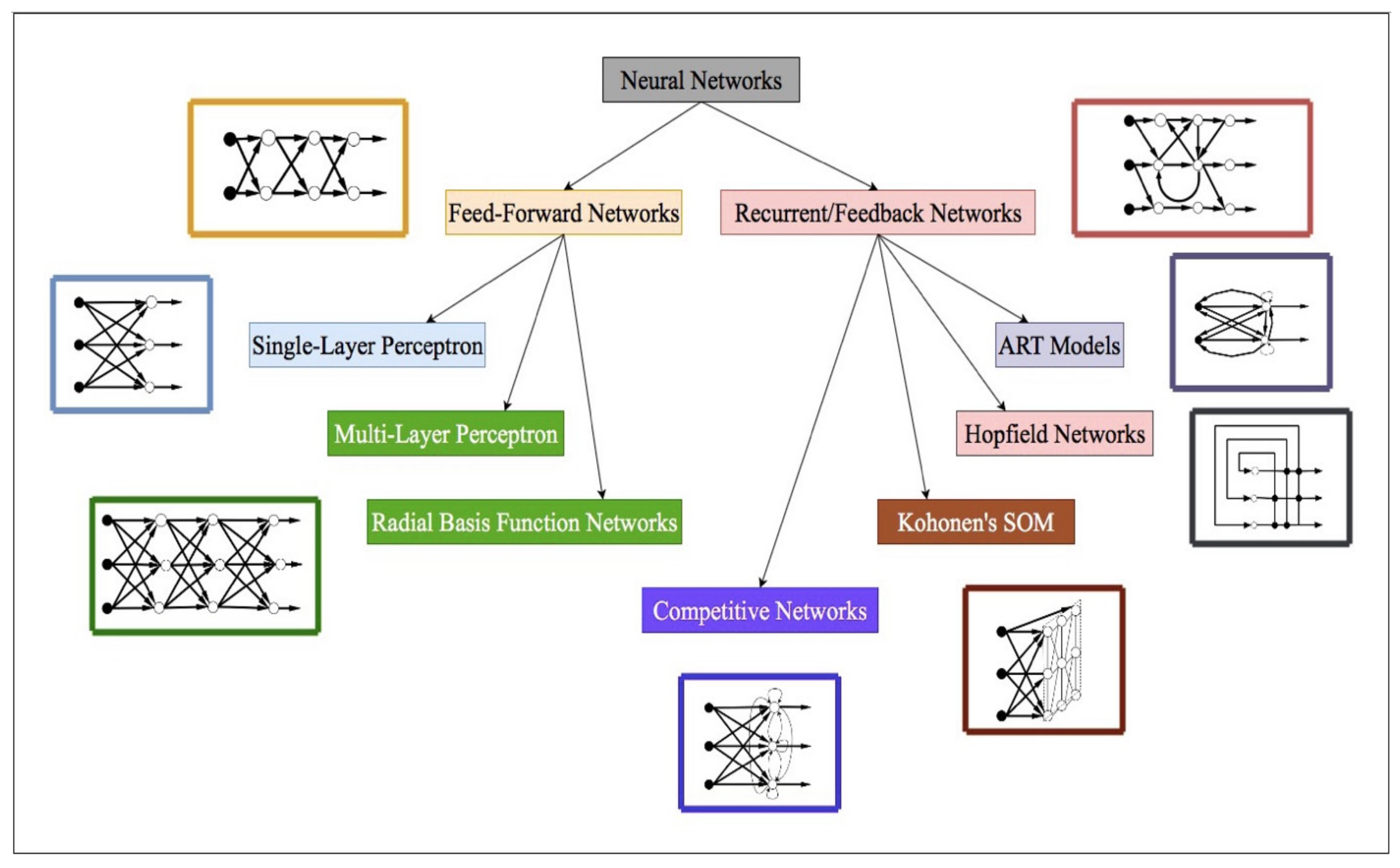
Figure 1. Basic structure of neural network.
Sustainability 12 04359 g001
Figure 2. Classification of neural network [66].
Sustainability 12 04359 g002
Figure 3. Comparison of nitrate-nitrogen in rivers for two decades of data [76].
Sustainability 12 04359 g003
Figure 4. (a) Classification of different point sources showing their contribution of ammonia-nitrogen in the Langat River; (b) comparison of the contributions of ammonia-nitrogen from point and non-point sources [41,79].
Sustainability 12 04359 g004
Figure 5. Comparison of 13 different models results with the DONcal.
Sustainability 12 04359 g005
Table 1. Advantages and disadvantages of different ANN (artificial neural network) models.
Main TypeModel NameAdvantagesDisadvantages
FFNN
(Feed-Forward Neural Network)
Single Layer Perceptron
  • Less computation—time

Easy to setup
  • Can only be used in linearly separable data
Multi-Layer Perceptron
  • Can be used for complex problems
  • Need more time for training
  • Can get stuck in local minima
RBFNN
  • Less susceptible to be stuck in local minima
  • Can tolerate with input noise
  • Classification is slow, as the network have to calculate the radial basis function for each input vector during classification
Recurrent/Feedback NetworkART (Adaptive Resonance Theory) model
  • Can be integrated with other models to enhance the performance
  • Some ART models are inconsistent. They depend upon the order of the training data
Hopfield Network
  • No training needed
  • Handles a smaller number of memories.
  • More number of patterns results in spurious output
Kohonen’s SOM
  • Provides deterministic and reproducible results
  • Simplicity of computation
  • Performance depends on initialization
Competitive Network
  • Groups the similar pattern based on the data correlation
  • Susceptible to stability issue
Table 2. A summary of studies that utilize ANN model for nitrogen prediction, including their specific area, location, and methods used.
AuthorsSpecific AreaLocationMethod
1Anctil, Filion and Tournebize [61]StreamsMelarchez, FranceStacked multilayer perceptron
2He, Oki, Sun, Komori, Kanae, Wang, Kim and Yamazaki [18]StreamsJapanFeed-forward model
3Holmberg, Forsius, Starr and Huttunen [19]StreamsFinlandBackpropagation algorithm
4Lek, Guiresse and Giraudel [20]StreamsThe United StatesMultilayer feed-forward
5Suen and Eheart [25]StreamsIllinois, The United StatesBackpropagation and radial basis
6Sharma, Negi, Rudra and Yang [6]Drainage waterCanadaFast backpropagation and self-organizing radial basis
7Wang et al. [86]GroundwaterAustralia13 machine learning models
8Zhang et al. [87]LakeChinaARIMA, radial basis, and hybrid
9Markus et al. [88]StreamsIllinoisBackpropagation, Evolutionary Polynomial Regression (EPR), and Naïve Bayes Model (NBM)
10Amiri and Nakane [89]StreamJapanBackpropagation and Multiple Linear Regression (MLR)
11Zeleňáková et al. [90]StreamsSlovakiaDimensional analysis
Table 3. Details of methodology of the reviewed research work.
No.AuthorsDuration of DataData Pre-ProcessingInternal Parameters
1Anctil, Filion and Tournebize [61]1975–1993 (Daily)Standardization (linearly)2 Inputs, 12 hidden neurons
2He, Oki, Sun, Komori, Kanae, Wang, Kim and Yamazaki [18]1995 (Monthly)Sensitivity Analysis8 Inputs, 7 hidden neurons
3Holmberg, Forsius, Starr and Huttunen [19]1990–2000 (Daily)-13 Inputs, 1 hidden layer, 7 nodes
4Lek, Guiresse and Giraudel [20]One yearSensitivity Analysis, Autoscaling8 Input, 10 hidden neurons
5Suen and Eheart [25]1993–2000, (Daily)--
6Sharma, Negi, Rudra and Yang [6]1991–1994, (Daily)Sensitivity AnalysisFast Backpropagation:
8 Inputs, 20 hidden neurons, learning rate: 0.02
RBFNN: Tolerance 20, spread 15
7Wang, Oldham and Hipsey [86]2006–2014,
(401 samples)
--
8Zhang, Zhang and Li [87]2006–2011, (Monthly)-ARIMA:
  • Nitrogen: p = 1, d = 1, q = 1
  • Phosphorus: p = 2, d = 1, q = 1
RBFNN:
  • 2 hidden layers
  • Training width σ = 0.6
9Markus, Hejazi, Bajcsy, Giustolisi and Savic [88]1994–1999, (Weekly)-ANN:
4 Input, 2 hidden nodes, epochs: 100,000; performance gradient: 1E-10; goal: zero
EPR equations:
N t + 1 = 0.827 N t
N t + 1 = 0.659 N t + 0.560 N t Q t
NBM equations:
N t + 1 = f N t ,   Q t ,   P t ,   T t
N t + 1 = f N t ,   Q t ,   Q t 1 ,   P t ,   P t 1 ,   T t ,   T t 1
10Amiri and Nakane [89]2001, (Monthly)Statistical Analysis6 Input nodes, 2 hidden nodes, 1 output nodes, 11,600 epochs
11Zeleňáková, Čarnogurská, Šlezingr and Słyś [90]2003–2010, (Monthly)Sensitivity AnalysisDimensional analysis equations:
π 1 = 0.0039 π 2 13.805
π 1 = 0.1868 π 2 9.7892
Table 4. A summary of studies that utilize ANN model for nitrogen prediction, including their input variables, prediction variables, and accuracy.
No.AuthorsInput VariablesPrediction VariablesAccuracy
1Anctil, Filion and Tournebize [61]
  • Same-day stream flow
  • Same-day 80 cm-depth soil moisture index
Nitrate-nitrogen fluxEfficiency index = 0.888
2He, Oki, Sun, Komori, Kanae, Wang, Kim and Yamazaki [18]
  • River discharge
  • Average temperature and precipitation of each basin
  • Amount of fertilizer applied in each basin
  • Proportions of forest land area, urban land area, road area, and other areas in the total basin area
Monthly total nitrogen concentrations R t r a i n i n g 2 = 0.96
R V a l i d a t i o n 2 = 0.84
R O v e r f i t t i n g 2 = 0.9
3Holmberg, Forsius, Starr and Huttunen [19]
  • Month of data sampling
  • Mean temperatures of 3 and 10 preceding days
  • Runoff of sampling day
  • Maximum and minimum runoffs of 3 preceding days
  • Days of peak flow, days of low flow
  • Catchment area
  • Fractions of lake area and peatland area with respect to catchment area
  • Catchment latitude and elevation
  • Total organic carbon
  • Total nitrogen
  • Total phosphorus
Flux efficiency:
  • Total organic carbon = 0.94
  • Total nitrogen = 0.92
  • Total phosphorus = 0.90
4Lek, Guiresse and Giraudel [20]
  • Average annual flow
  • Animal unit density
  • Mean annual streamflow
  • Percentage of forest cover, wetland, urban, agriculture and the percentage of remaining area in the catchment
Inorganic and total nitrogen concentration Correlation coefficient:
Total nitrogen = 0.82
Inorganic nitrogen = 0.8
5Suen and Eheart [25]
  • Daily highest temperature
  • Seven-day cumulative daily rainfall
  • Daily streamflow
  • Julian date
Nitrate concentrationOverall accuracy:
  • Method one:
  • BPNN = 0.784
  • RBFNN = 0.752
  • Method two:
  • BPNN = 0.832
  • RBFNN = 0.832
  • Boolean output (Method two)
  • BPNN = 0.866
  • RBFNN = 0.893
6Sharma, Negi, Rudra and Yang [6]
  • Treatment
  • Julian day
  • Rainfall per day
  • Cumulative rainfall
  • Total nitrogen applied
  • Snowfall per day
  • Maximum and minimum temperature
Nitrate concentrationCorrelation coefficient
  • RBFNN
  • Tillage = 0.8079
  • No tillage = 0.6911
  • BPNN
  • Tillage = 0.8017
  • No tillage = 0.6635
7Wang, Oldham and Hipsey [86]
  • Scenario 1
  • Nutrients (dissolved organic nitrogen (DON), total nitrogen, N H 4 + , N O x )
  • Landscape (vegetation, land use, and soil)
  • Hydrological conditions (surface water subarea, groundwater subarea, and catchment area)
  • Sampling condition (temperature, sample depth, and sampling date, pH)
  • Scenario 2
  • Total nitrogen
  • All other non-nutrient data
DONR2 of best models:
  • Scenario 1
  • Cubist = 0.897
  • Bagged multivariate adaptive regression spline (Bagged mars) = 0.882
  • Random forest (RF) = 0.856
  • Scenario 2
  • Cubist = 0.849
  • Bagged mars = 0.887
  • RF = 0.858
8Zhang, Zhang and Li [87]Monthly data for total nitrogen
  • Monthly total nitrogen
  • Monthly total phosphorus
Mean absolute percentage error:
  • Nitrogen
  • ARIMA = 18.194%
  • RBFNN = 34.633%
  • Hybrid = 7.017%
  • Phosphorus
  • ARIMA = 27.299%
  • RBFNN = 126.957%
  • Hybrid = 14.528%
9Markus, Hejazi, Bajcsy, Giustolisi and Savic [88]
  • Observed weekly river discharge
  • Precipitation
  • Air temperature
  • Nitrate-nitrogen concentration
  • Weekly nitrate-nitrogen
Root mean square error (RMSE) for ANN:
  • Training = 0.787 mg/L
  • Testing = 0.935 mg/L

RMSE for EPR:
  • Training = 0.991 mg/L
  • Testing = 1.010 mg/L

Critical success index for NBM:
  • NBM1:
  • Training = 0.214
  • Testing = 0.200
  • NBM2:
  • Training = 0.286
  • Testing = 0.188
10Amiri and Nakane [89]
  • Percentage land use
  • Urban
  • Forest
  • Agriculture
  • Grassland
  • Water body
  • Population density
Total nitrogenR2 Value:
  • BPNN = 0.94
  • MLR = 0.85
11Zeleňáková, Čarnogurská, Šlezingr and Słyś [90]
  • Stream discharge
  • Catchment area
  • Stream velocity
  • Temperature of air and water
  • Concentration of pollutant
Nitrogen and phosphorus concentrationAverage Uncertainty:
  • Nitrogen = 31.33%
  • Phosphorus = 32.30%

