Car-Access Attractiveness of Urban Districts Regarding Shopping and Working Trips for Usage in E-Mobility Traffic Simulations

Abstract

With the continuous proliferation of private battery electric vehicles, the demand for electrical energy and power is constantly increasing. As a result, the electrical grid may need to be expanded. To plan for such expansion, information about the spatial distribution of the energy demand is necessary. This can be determined from e-mobility traffic simulations, where travel schedules of individuals are combined with an attractiveness rating of locations to estimate traffic flows. Typically, attractiveness is determined from the “size” of locations (e.g., number of employees or sales area), which is applicable when all modes of transportation are considered. This approach leads to inaccuracies for the estimation of car traffic flows, since the parking situation is neglected. To overcome these inaccuracies and fill this research gap, we have developed a method to determine the car-access attractiveness of districts for shopping and working trips. Our method consists of two steps. First, we determine the car-access attractiveness of buildings within a district based on the parking situation of each individual building and then aggregate the results at the district level. The approach is demonstrated for the city of Berlin. The results confirm that conventional models cannot be used to determine the car-access attractiveness of districts. According to these models, attractive districts are predominantly located in the city centre due to the large amount of sales areas or the large number of employees. However, due to the high density of buildings, only limited space is available for parking. Attractive districts rated according to our new approach are mainly located in the outer areas of the city and thus match the parking situation.

1. Introduction

This introduction consists of three subsections. In Section 1.1, we discuss how the conversion from private internal combustion engine vehicles (ICEVs) to battery electric vehicles (BEVs) contributes to a reduction in greenhouse gas emission. Furthermore, we discuss how e-mobility traffic simulations are used to estimate the spatial and temporal distribution of the charging demand of BEVs and why these simulations are necessary. Since the currently used models rely on data that is not always available, we have developed a novel research approach to estimate the charging demand of BEVs. This is presented in Section 1.2. This paper is one of three main parts that together form the research approach. Therefore, this subsection also discusses which part of the overall research approach is addressed in this paper. In Section 1.3, a literature review about the car-access attractiveness of locations is conducted, and the research gap filled by this paper is identified.

1.1. Global Warming and E-Mobility Traffic Simulations to Estimate the Charging Demand of BEVs

In recent years, emission limits have been steadily tightened due to continuously rising greenhouse gas emissions and poor air quality. Germany, for example, is planning to reduce greenhouse gas emissions by 50% by 2030 compared to 1990 [1]. The European Commission agreed on the “European Green Deal”, with the intention to achieve net zero greenhouse gases emissions by 2050. To achieve this goal, “a 90% reduction in transport emissions is needed by 2050” [2]. This reduction leads to a substitution of private internal combustion engine vehicles with vehicles with alternative drive systems, primarily battery electric vehicles. As a result, the increasing demand for electrical energy and power can lead to bottlenecks in the power supply if the electrical grid infrastructure is not reinforced [3,4]. In order to support the electrical grid operators to detect and evaluate possible overloads within the electrical grid, accurate models are needed to predict the spatial and temporal energy and power requirements arising from the electrification of private internal combustion engine vehicles.

E-mobility traffic simulations, mostly in the form of activity-based models, are commonly used for this purpose [5,6,7,8]. In activity-based models, individual full-day travel schedules are generated for all persons or vehicles within the considered geographical area. These travel schedules, also referred to as mobility profiles, consist of a consecutive sequence of activities at different locations and trips between those activities. An example of a mobility profile is shown in Figure 1, where the individual starts at ”Home” in the morning before spending 8 h and 30 min at the activity “Working” and 40 min at the activity “Shopping”. The person arrives back “Home” at 18:00.

Since the mobility profiles capture the relationship between activity and mobility patterns and mode of transportation, they can be used to determine the idle times of the vehicles at different activities. If the geographic locations of the activities are known, the spatial and temporal distribution of the charging energy and power demand for a geographic area can be calculated from the mobility profiles by applying charging strategies.

In activity-based models, the standard approach to determine mobility profiles containing information about the activity locations is to combine a travel survey with an origin-destination (O-D) matrix [6,7]. The travel surveys are obtained by questioning households within a geographical area about their activities and trips during reference days, which allows for determining the daily travel patterns of the population in the investigated area. An O-D matrix is then used to derive the locations of the activities. In O-D matrices, each cell represents the probability of a trip from an origin location (row) to a destination location (column) within a geographical area. As the starting location of the first trip (usually the “Home” location) is known through, e.g., statistics on population density or the degree of motorisation, O-D matrices are used to assign the destination locations for different activities. In some cases, travel surveys contain sufficient data to directly derive an O-D matrix [6,7]. If the data availability is insufficient, O-D matrices have to be generated by other approaches, usually by using traffic count data [9,10,11,12] or mobile phone data [13,14,15].

1.2. Novel Research Approach for Estimating the Charging Demand of BEVs

In the case where an O-D matrix neither exists nor can be determined, we have developed a new approach which can be used to determine mobility profiles containing information about the activity locations for the considered geographical area. This approach is depicted in Figure 2. As a first step (depicted in the blue box), a travel survey is used to create mobility profiles that do not contain information about the activity locations. The mobility profiles are vehicle-based and not person-based. This means that individual travel schedules are created for BEVs in the geographic area and not for persons. In this way, the multiple use of the same vehicle by several people can be realistically represented. Population density statistics as well as data on the degree of motorisation are used to determine the residence of the individuals and thus the spatial distribution of the vehicles in the investigated area. From the spatial distribution of household incomes, vehicle size classes and therefore vehicle consumption can be determined. Based on these partial results, it is possible to estimate the spatial distribution of the charging energy and power demand that arises when the individuals solely charge their BEVs at home. This approach has been demonstrated in [5] for the urban area of Berlin, Germany, and its 448 sub-districts. However, these results need further refinement as they neglect the fact that vehicles do not always charge at home but can also charge at, e.g., work and shopping locations.

Therefore, as second step we determine the car-access attractiveness of locations, as depicted in the orange box of Figure 2. Car-access attractiveness is a measure of how attractive locations are to drive to by car for a certain activity. A high attractiveness means that a location is highly likely to be accessed by car, while a low attractiveness indicates that a location is more likely to be accessed by another mode of transportation. In order to determine the car-access attractiveness of a location for a certain activity, the performed activities at each location need to be known. Therefore, the usage of each building in the investigated area is first determined and then the car-access attractiveness of each building is computed based on its usage and parking situation. The results for the buildings are subsequently aggregated at the district level. In the last step, the attractiveness information and the mobility profiles without information about the activity locations are combined with a suitable routing method. The routing of the vehicles allows for determining the locations of the activities based on the location attractiveness. This enables the estimation of the spatial distribution of the charging energy and power demand, considering charging at all activities. Whereas the routing method will be part of future work, this paper deals with the evaluation of the car-access attractiveness of buildings and districts.

1.3. Literature Review and Research Gap Filled by This Paper

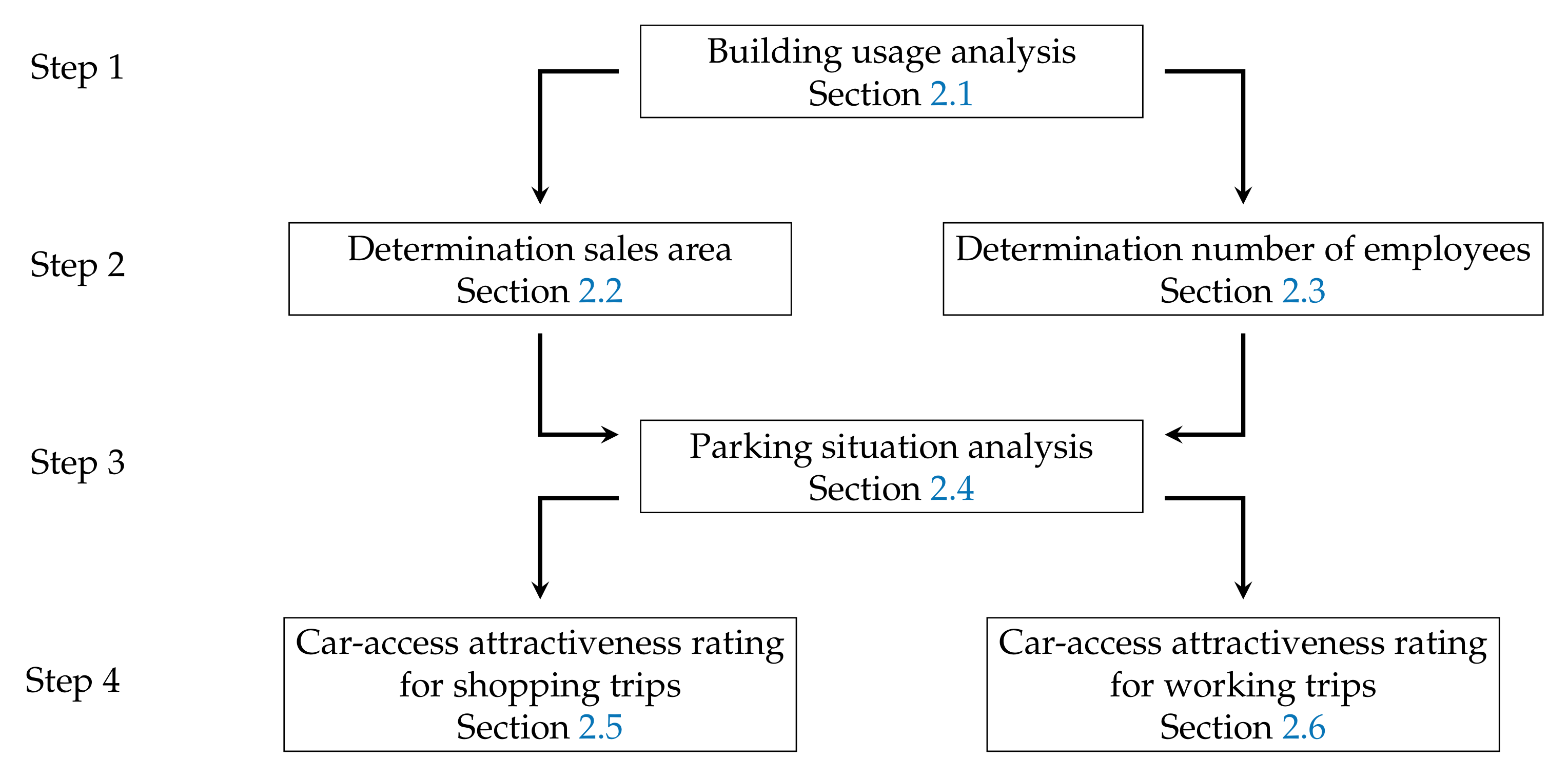
Typically, attractiveness is represented by the “size” of locations, assuming that larger places attract more persons than smaller ones [16]. Horni et al. [17] as well as Kubis and Hartmann [18] proposed an attractiveness factor depending on store size to model the location choice of individuals for shopping trips. They assume that larger stores attract more persons than smaller ones. In order to relate retailing attractiveness of an urban district with its resulting freight and shopping trip attraction rates, Gonzalez-Feliu and Peris-Pla [19] assume that districts with a high number of employees attract more trips as their attractiveness increases. Caceres et al. [20] assume that districts with high population attract more trips and propose a relative attractiveness factor to estimate traffic flow profiles. Drezner and Drezner [21] propose that the annual sales of a retail facility indicate its attractiveness.

The described models can only be applied when all modes of transport are considered. They cannot be applied when cars are the only mode of transport under consideration. This is mostly because these models do not consider the availability of parking spaces. An example is that of large department stores, which are usually located in the city centres. Since they offer a large amount of sales area, they are characterized by very high car-access attractiveness if evaluated with conventional attractiveness models. However, within the city centres, usually limited or no space is available for parking.

Since the evaluation of the car-access attractiveness of locations has not been addressed so far in the literature, this research gap is filled by this paper. The car-access attractiveness is evaluated separately for shopping and working trips and is based on the consideration of the available parking space in relation to the sales area per district and the number of employees per district, respectively. To refine our attractiveness rating, we also consider the distance of the parking spaces from the shops and working locations, the distance of the working location to the nearest public transportation stop and information about the parking fees. We apply our method to the urban area of Berlin, Germany, and its 448 sub-districts. The car-access attractiveness rating is based on open geodata and freely available data sets, making the approach traceable and reproducible.

Since the car-access attractiveness of the districts is determined solely for shopping and work trips, vehicle routing can only determine the locations for shopping and work activities. However, in addition to the places of residence, these are the locations with the highest charging potential, as they have the highest average car idle times in Berlin (places of residence: 20.9 h per day, workplaces: 1.7 h and shopping locations: 0.1 h) [5].

This paper is structured as follows: in Section 2, the method for the attractiveness-based district rating is introduced. The results are presented and analysed in Section 3, which is divided into two main parts. In Section 3.1, the results of the attractiveness-based district rating are shown for shopping trips. The results are shown for working trips in Section 3.2. The conclusions are presented in Section 4.

2. Methodology

The methodology used to rate districts regarding their car-access attractiveness consists of four main parts, which are depicted in Figure 3. As a first step, we divide the city of Berlin into districts and analyse the usage of each building inside the districts. The building usage describes how the building is used, e.g., as a commercial or residential building. For the division we make use of the official classification of the Berlin administration, which divides the twelve Berlin districts into 448 sub-districts called ”Lebensweltlich orientierte Räume“ (Eng.: neighbourhood-oriented districts, abbr.: LORs). Within each LOR, the structure of the contained buildings and the socio-economic status of the inhabitants are similar. The LORs are usually separated from each other by major roads, rivers or rails [22,23]. The analysis of the buildings’ usage is based on geodata, which is information about geographic positions in a computer-processable format. For the analysis of the buildings’ usage within the LORs, we use OpenStreetMap (OSM) geodata [24], derived from the Geofabrik GmbH Karlsruhe [25]. We chose OSM geodata because it is freely available under an open database license 1.0 [26] for the whole earth. The car-access attractiveness of a district is based on the available parking space in relation to the sales area per district and the number of employees per district, respectively. Therefore, in the second step we use the results of the building usage analysis to derive the sales area and the number of employees for all buildings in the Berlin LORs. We analyse the parking space availability in the Berlin LORs in step three. As a last step, we combine the obtained results and introduce the methodology for the attractiveness-based district rating.

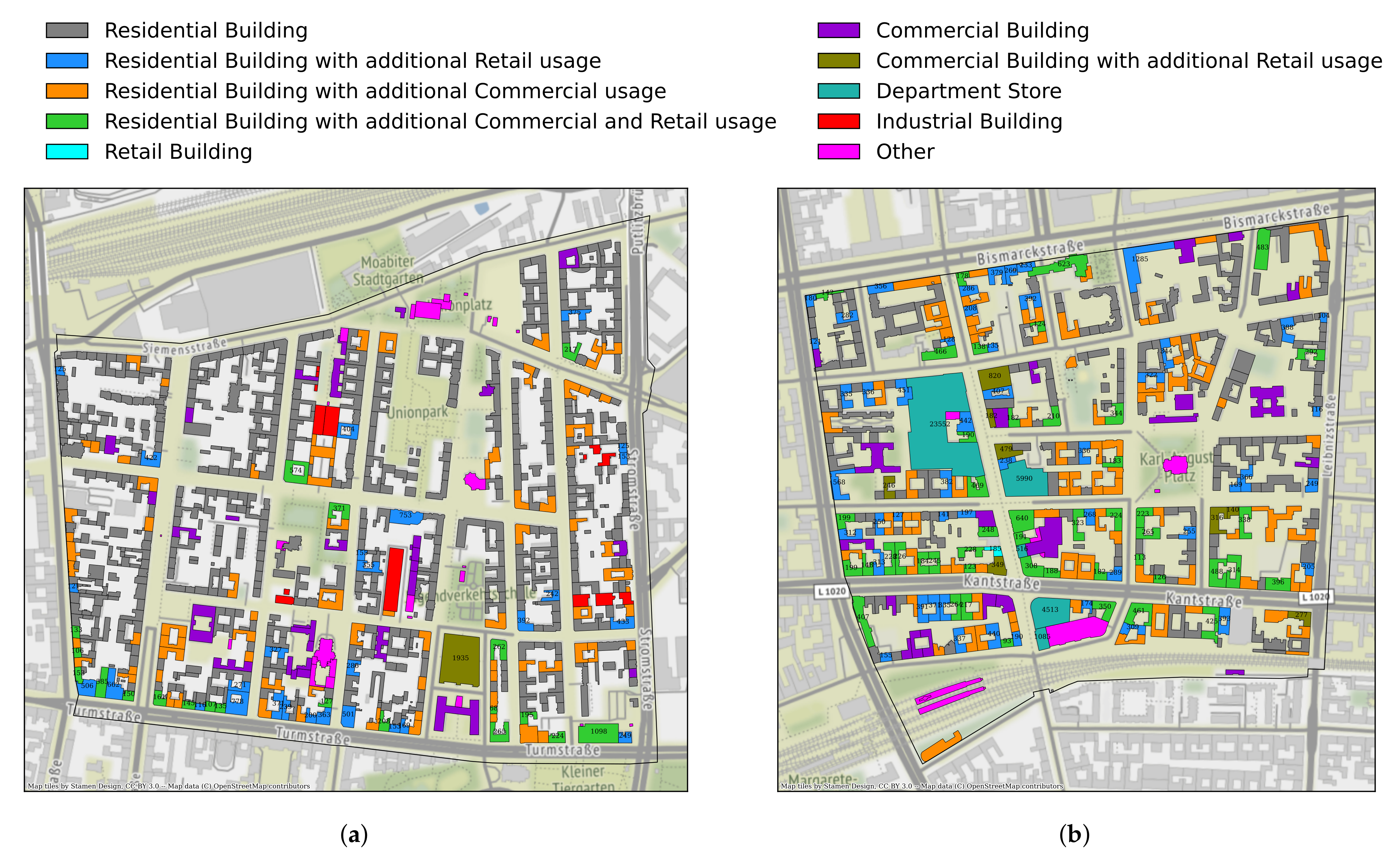
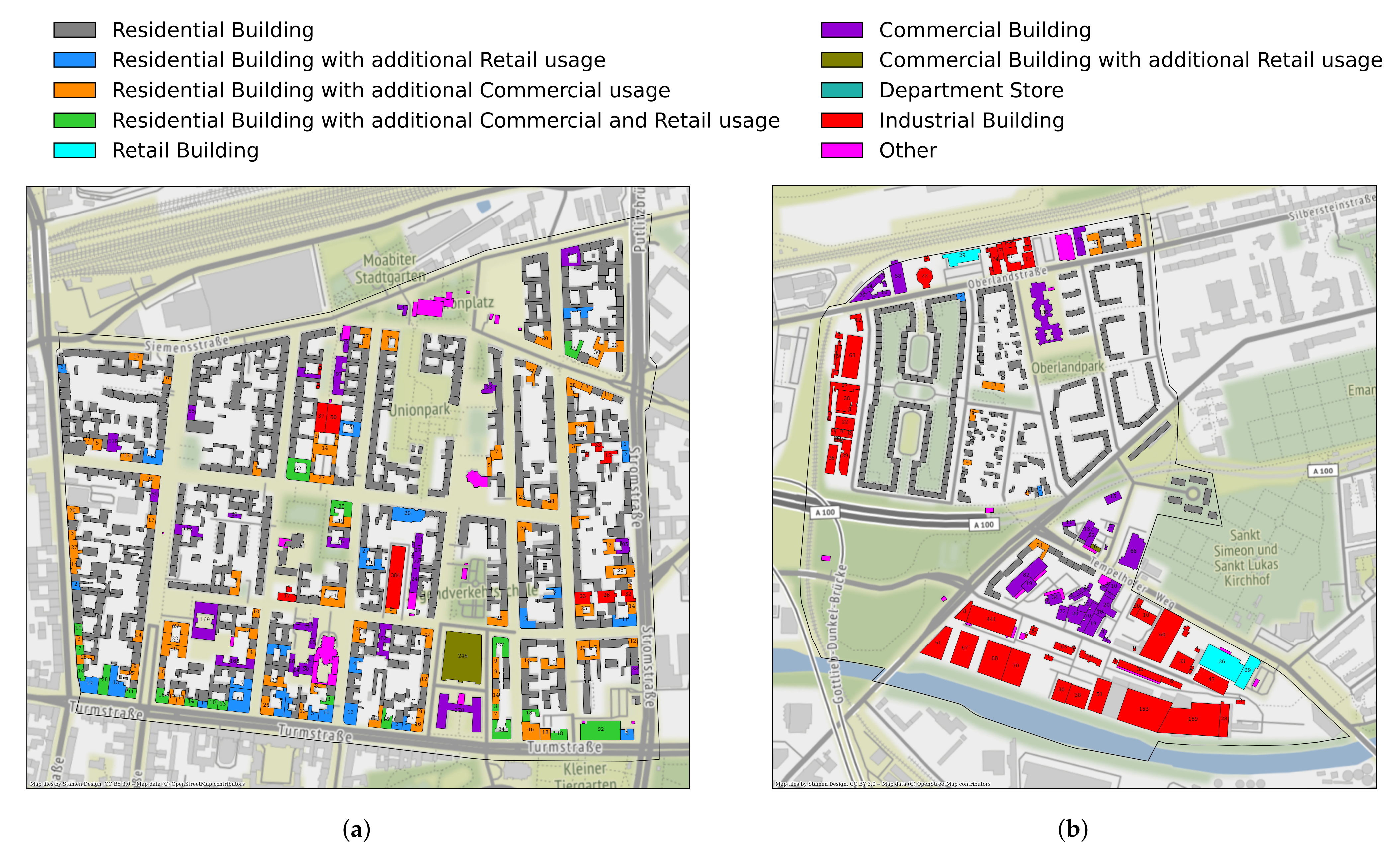
2.1. Building Usage Analysis in the Berlin LORs

In this section, we derive the building’s usage for every building inside the Berlin LORs. Additionally, we determine the number of floors for each building, which is necessary to compute the sales area and the number of employees per building. For the building usage analysis we solely rely on OSM raw data, which is xml-formatted. The OSM raw data structure is composed of the three elements—“nodes”, “ways” and “relations”—as well as “tags” associated with the elements [27].

• “Nodes” are points defined by their latitude and longitude and therefore correspond to locations on the surface of the earth.
• “Ways” are ordered lists of nodes. Up to 2000 nodes define a polyline, which can be used to define linear features (e.g., rivers or roads) or boundaries of areas in the form of a polygon (e.g., buildings or parking spaces).
• “Relations” are used to model logical or geographical relationships between elements.
• “Tags” describe the element they are attached to. A tag consists of a key and a value. For example, a supermarket would be assigned the key =“shop” and the value =“supermarket”.

For each building, three main pieces of information can be obtained from the OSM data set: firstly, the predominant land use of the area the building lies in (e.g., residential, industrial or retail land use); secondly, the building type such as an office, church or residential building; and thirdly the points of interest (POIs) within the building. While the land use and the building type are mainly given as polygons, POIs are usually given as nodes and give deeper insights into the building’s usage.

The Berlin OSM geodata set includes 19 different land uses, 191 different building types and 852 different POIs. Conditions are defined to categorize the Berlin buildings into their corresponding building usage class, taking the buildings land use, type and POIs within it into account. For example, if no POI is given and the building’s land use and the building’s type are “residential”, the building is considered as a residential building. The POI “supermarket” within a building of the land use and building type “residential” would reveal that a supermarket is located inside the building, and the building would be considered as a residential building with additional retail usage. For the categorization, we consider 10 different building usage classes in total:

• Residential buildings;
• Residential buildings with additional commercial usage, such as small offices or doctor’s practices;
• Residential buildings with additional retail usage, such as small supermarkets or bakeries;
• Residential buildings with additional commercial and retail usage;
• Commercial buildings, such as an office building;
• Retail buildings, such as supermarkets or furniture stores;
• Commercial buildings with additional retail usage;
• Industrial buildings, such as factories;
• Department stores;
• Others, such as churches, monuments or stadiums.

The number of floors can be directly derived from the OSM geodata set for most Berlin buildings. However, since the data set is not complete, the floor numbers for the buildings without information need to be determined. The Berlin LORs are defined in such a way that the building structure within each LOR is similar [22,23]; hence, the number of floors of the buildings is similar. Therefore, we estimate the number of floors for buildings without information by calculating the average number of floors for each building usage class in the LOR and assign the results to buildings without information.

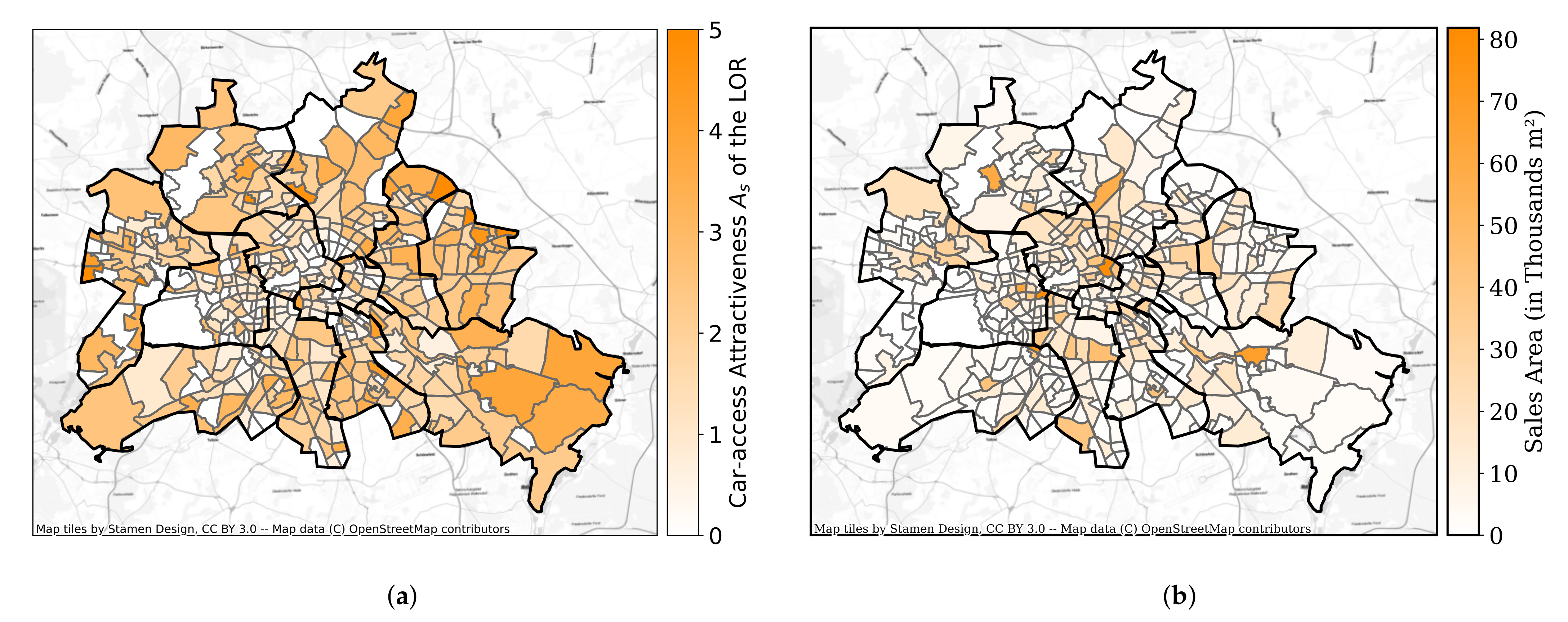
2.2. Determination of the Sales Area of the Buildings in the Berlin LORs

In order to calculate the sales area of a building, two major pieces of information need to be known: namely, the sales area per floor and the number of floors within the building containing sales areas. To derive the relevant information for a building, we make use of its usage class and its number of floors, derived in Section 2.1. We calculate sales areas for the following building usage classes:

• Residential buildings with additional retail usage;
• Residential buildings with additional commercial and retail usage;
• Retail buildings;
• Commercial buildings with additional retail usage;
• Department stores.

As the OSM data set reveals no information concerning the number of floors per building that contain sales area, we assume that for a residential and a commercial building with additional retail usage, only one floor contains sales area. For retail buildings and department stores, we assume that each floor contains sales area. We further assume that each floor contains the same amount of sales area. To avoid overestimating the sales areas of department stores with additional commercial usage such as offices or a hotel, we limit the number of floors containing sales area to two floors for those.

Two steps are then necessary to derive the sales area per floor from the gross floor area of a building. First, the net internal area needs to be calculated. The net internal area equals the gross floor area minus the area used for, e.g., stairs and elevators, electrical services or walls and columns. As second step, the sales area needs to be determined from the net internal area. The sales area only contains the shelf areas and the paths running between them, as well as counters and the checkout area. The sales area does not include storage areas or administration offices. For Germany, Tillman et al. [28] have published guideline factors to derive the net internal area from the gross floor area for residential and commercial buildings. For both building types, this factor $K_1$ can be computed as

$$K_1=\frac{\mathrm{Net}\mathrm{Internal}\mathrm{Area}}{\mathrm{Gross}\mathrm{Floor}\mathrm{Area}}=0.8$$

(1)

The authors additionally provided a guideline factor of $K_2=0.8$ for the estimation of the sales area from the net internal area, resulting in a total factor of $K_3=0.64$ for the estimation of the sales area from the gross floor area.

$$K_2=\frac{\mathrm{Sales}\mathrm{Area}}{\mathrm{Net}\mathrm{Internal}\mathrm{Area}}=0.8$$

(2)

$$K_3=K_1·K_2=\frac{\mathrm{Sales}\mathrm{Area}}{\mathrm{Gross}\mathrm{Floor}\mathrm{Area}}=0.64$$

(3)

While the factor $K_2$ is also applicable for the usage classes “retail building” and “department store”, no values are available to estimate the net internal area from the gross floor area for these two usage classes. We therefore assume $K_1=0.8$ as well for these building usage classes. To check this assumption, we compare the calculated sales areas of retail buildings and department stores with reference values in the following. As Berlin is highly populated and construction land is rare, pure retail buildings are uncommon. The few that exist are mostly supermarkets. Accordingly, we take Aldi Nord and Kaufland supermarkets into account for the comparison. Aldi Nord supermarkets are chosen for the verification, since they offer an “average” product assortment on an average sales area size of 850 m${}^2$ and hence can be considered as an “average” Berlin supermarket [29]. Kaufland supermarkets are chosen, since they offer a wide product assortment on large sales areas of 4340 m${}^2$ on average [30] and therefore differ in means of building structure compared to Aldi Nord supermarkets. Thus, they provide a useful second comparison value. The results of the comparison are depicted in

Table A1. Comparison of the average sales area of retail buildings and the total sales area of three department stores with computed values.

Building Usage Class	Type	Average/ Total Sales Area (m${}^2$)	Average/ Total Computed Sales Area (m${}^2$)	Relative Error (%)
Retail Building	Aldi Nord [29]	850	826	−2.8
	Kaufland [30]	4340	4390	−1.1
Department Store	Wima Shopping [52]	25,000	23,552	−5.8
	Spandauer Arcarden [53]	33,000	32,046	−2.9
	Bikini Berlin [54]	17,000	17,954	5.6

. Since the relative error between the computed average sales area and its reference value is −2.8% for Aldi Nord supermarkets and −1.1% for Kaufland supermarkets, we consider a factor of $K_3=0.64$ as applicable to derive the sales area from the gross floor area for retail buildings. For department stores, we verify the assumption by comparing the calculated sales areas with known numbers for 15 department stores in Berlin. As the calculated mean relative error is 4.2%, we assume an applicability of the factor $K_3=0.64$ to derive the sales area from the gross floor area for department stores as well. The results of the comparison are depicted for three departments stores in Table A1.

The computed total sales areas for the Berlin buildings needs to be verified. Therefore, we compare our computed results with a study on Berlin retail structures and sales areas, commissioned by Berlin authorities in 2014 [31]. The study provides information on the sales area per inhabitant in the 12 Berlin districts in the year 2016. In order to calculate the sales area per district, we use census data, which provides the number of inhabitants for the Berlin districts in 2016 [32]. The number of inhabitants in Berlin has grown by 1.9% from 3,537,100 in 2016 [32] to 3,604,100 in 2019 [33]. Accordingly, we assume that the total sales area increased by 1.9% from 2016 to 2019. The results of the comparison can be found in

Table A2. Sales area per district; comparison of authority data with computed values.

District	Inhabitants	Sales Area per Inhabitant (m${}^2$)	Total Sales Area (m${}^2$)	Computed Sales Area (m${}^2$)	Relative Error (%)
Mitte	375,500	1.79	672,145	691,234	2.8
Friedrichshain-Kreuzberg	275,400	0.86	236,844	246,543	4.1
Pankow	395,100	1.14	450,414	435,786	−3.2
Charlottenburg-Wilmersdorf	317,100	1.55	491,505	485,342	−1.3
Spandau	237,400	1.29	306,246	288,523	−5.8
Steglitz-Zehlendorf	289,600	1.16	335,936	349,876	4.1
Tempelhof-Schöneberg	340,300	1.47	500,241	451,478	−9.7
Neukölln	318,000	1.09	346,620	334,893	−3.4
Treptow-Köpenick	265,500	1.15	305,325	298,652	−2.2
Marzahl-Hellersdorf	255,800	1.24	317,192	267,639	4.6
Lichtenberg	278,900	0.91	253,799	261,757	3.1
Reinickendorf	255,700	1.02	260,814	255,739	−1.9

. The maximum relative error is 5.8% for all districts, except for the district Tempelhof-Schöneberg, indicating high accuracy of the computation. The high error of −9.7% in the district Tempelhof-Schöneberg is most likely due to the incomplete data set available for this district.

Figure 4 shows the computed sales area of each building in the LORs “Emdener Straße” and “Karl-August-Platz”. The usage distribution of the buildings in the LOR “Emdener Straße” can be considered as rather typical for Berlin. The LOR contains mostly residential buildings, intermixed with some commercial buildings and a main street (in the south of the LOR), where most of the buildings are used for retail or commercial purposes. The total sales area is 16,287 m${}^2$. In comparison, the buildings in the LOR “Karl-August-Platz” are mainly used for retail and commercial purposes. In addition, this LOR contains a shopping street with department stores. The total sales area is 66,555 m${}^2$.

2.3. Determination of the Number of Employees of the Buildings in the Berlin LORs

The calculation of the employees per building is carried out for each usage class introduced in Section 2.1, except for “residential buildings” and “other” usage classes, as they only have few or no employees. For the calculation, three major pieces of information need to be known: first, the number of companies per building, which we derived by analysing the POIs for each building; second, the number of employees per m${}^2$ of operating area for each company; and third, the share of the buildings operating area used by the individual companies. The total operating area of a building equals the gross floor area multiplied by the number of floors.

The number of employees per m${}^2$ of operating area $E_o$ can be directly derived for more than 30 types of businesses from [34]. Reference [34] is a study on the energy consumption of different economic sectors in Germany and also gives the average operating area $c_a$ of the business types. Exemplary values for five types of businesses can be found in

Table 1. Number of employees per m${}^2$ of operating area and average operating area for different types of businesses.

Type of Business	Employees per m${}^2$	Average
	Operating Area ${\mathit{E}}_{\mathit{o}}$	Operating Area ${\mathit{c}}_{\mathit{a}}$
Restaurants	0.023	260 m${}^2$
Retail non-food	0.011	530 m${}^2$
Insurances	0.036	477 m${}^2$
Small offices (e.g., law firm)	0.039	210 m${}^2$
Public institutions	0.019	2890 m${}^2$

.

According to the determination of the sales area per building, we limit the number of floors used by the companies to one for residential buildings with additional retail and/or commercial usage. If the building’s usage class is a retail building, a department store or an industrial building, we consider all floors of the building for commercial activities. We limit the number of floors of department stores with additional commercial usage to two. The remaining floors are treated as a commercial building. If several companies are located in the same building, the total operating area is distributed among the companies according to their weighted average operating area, as expressed in Equation (4).

$$O_i=O_t·\frac{c_{ai}}{{\displaystyle \sum _{j=1}^n}{c}_{aj}}$$

(4)

where $O_t$ is the building’s total operating area, $O_i$ the operating area of the company i located in the building and $c_{ai}$ is the average operating area of the company i, while n equals the total number of companies in the building and their corresponding average operating area $c_{aj}$.

Based on the values determined, the number of employees for all buildings in Berlin can be determined. For each building, its total number of employees $E_b$ can be calculated as

$$E_b=\sum _{i=1}^n{O}_i·E_{oi}$$

(5)

where $O_i$ is the operating area of the company i located in the building, and $E_{oi}$ is the number of employees per m${}^2$ of operating area of the company i, while n equals the total number of companies in the building.

In order to evaluate the generated results, we compare them to the 2019 Berlin census data [33]. The census data specify the total number of employees in Berlin and their distribution among three major commercial sectors: the manufacturing sector (e.g., automotive industry or chemical industry); the trade, hospitality and transport sector; and third, other commercial services sector (e.g., doctors or lawyers). The generated numbers from the OSM data, the numbers from the census and the relative error between them are depicted in

Table 2. Number of employees in Berlin in 2019 by summarized economic sector. Comparison of census data and computed results.

	Manufacturing Sector	Trade, Hospitality and Transport	Other Commercial Services	Total Number
Census Data	284,319	580,933	1,201,074	2,066,326
Computed Results	284,844	239,903	677,209	1,201,956
Relative Error (%)	0.185	−58.7	−43.6	−41.8

. The numbers of employees as derived from the census data are scaled to take commuters into account [35,36]. The computed total number of employees deviates by −41.8% compared to the census data. While the relative error is only 0.185% for the manufacturing sector, it is −58.7% for the trade, hospitality and transport sector and −43.6% for the other commercial services sector. Since OpenStreetMap is a community project, geographic data are collected on a voluntary basis by project members using their GPS devices [25]. Therefore, the large error for the trade, hospitality and transport sector and other commercial services sector is most likely due to the incompleteness of the OSM data set. The comparison of the OSM data with local knowledge confirms this assumption. Many small offices (e.g., architects, lawyers, consultancies), small doctor’s practices, restaurants or the offices of self-employed persons are not included in the data set, while large companies and factories of the manufacturing sector are fully included. In order to fit the calculated results to the census data, we linearly scale the computed results for each building with employees by economic sector.

The results of the determination of the number of employees are shown in Figure 5 for the LORs “Emdener Straße” and “Germaniagarten”. For each building, the calculated total number of employees is given. The usage of the buildings in the LOR “Emdener Straße” has been discussed in Section 2.2. The calculated total number of employees is 4901. Although the LOR “Germaniagarten” contains two industrial areas in the south and west as well as a commercial area in the centre, the number of employees in the LOR “Germaniagarten” is 3078 and thus is lower than in the LOR “Emdener Straße”. This is due to the fact that most of the industrial and commercial buildings in the LOR “Germaniagarten” have only one floor, while most buildings in the LOR “Emdener Straße” have more than two floors. Furthermore, industrial buildings have fewer employees per square metre operating area compared to buildings with solely or partly commercial usage which are common in the LOR “Emdener Straße”.

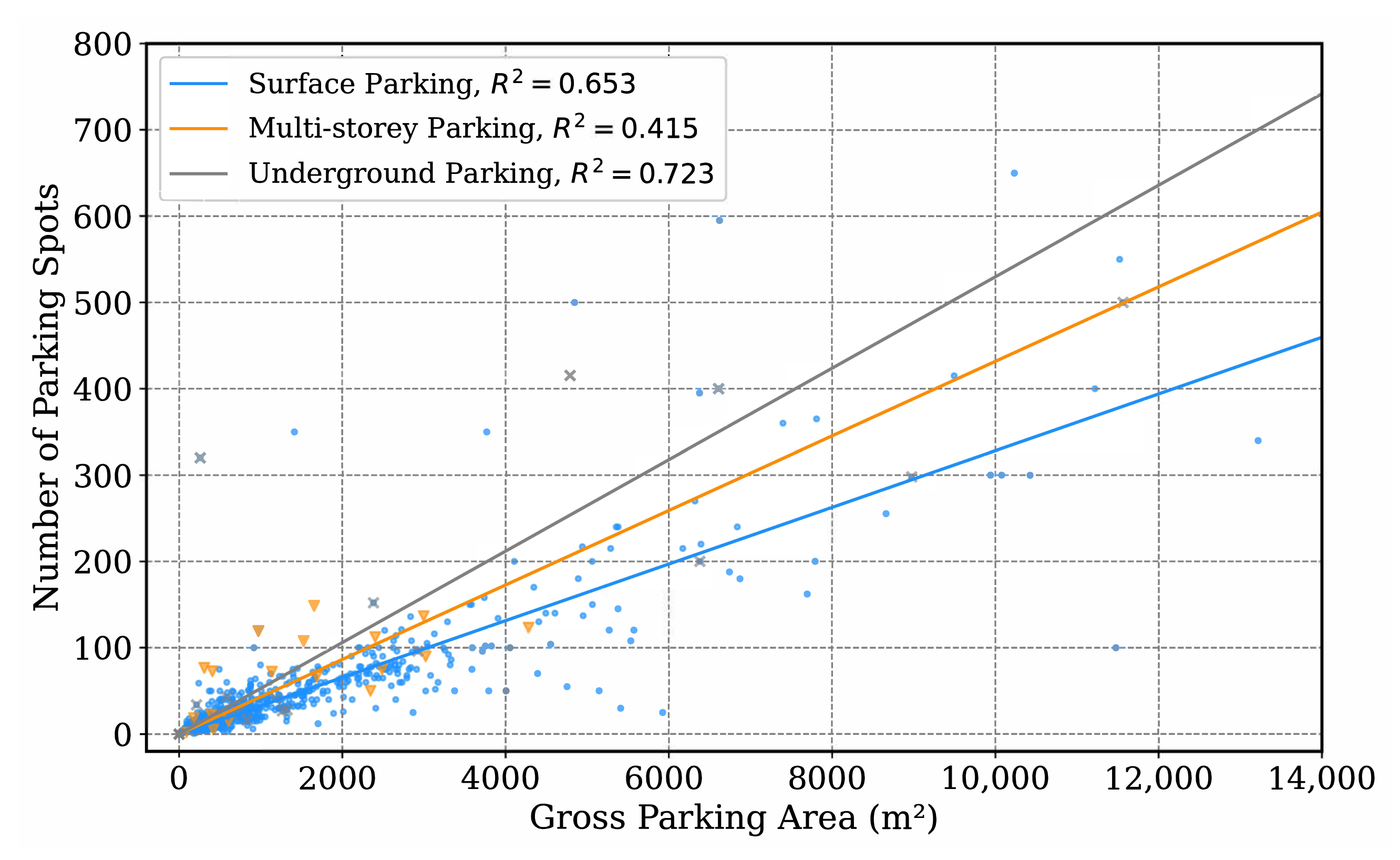
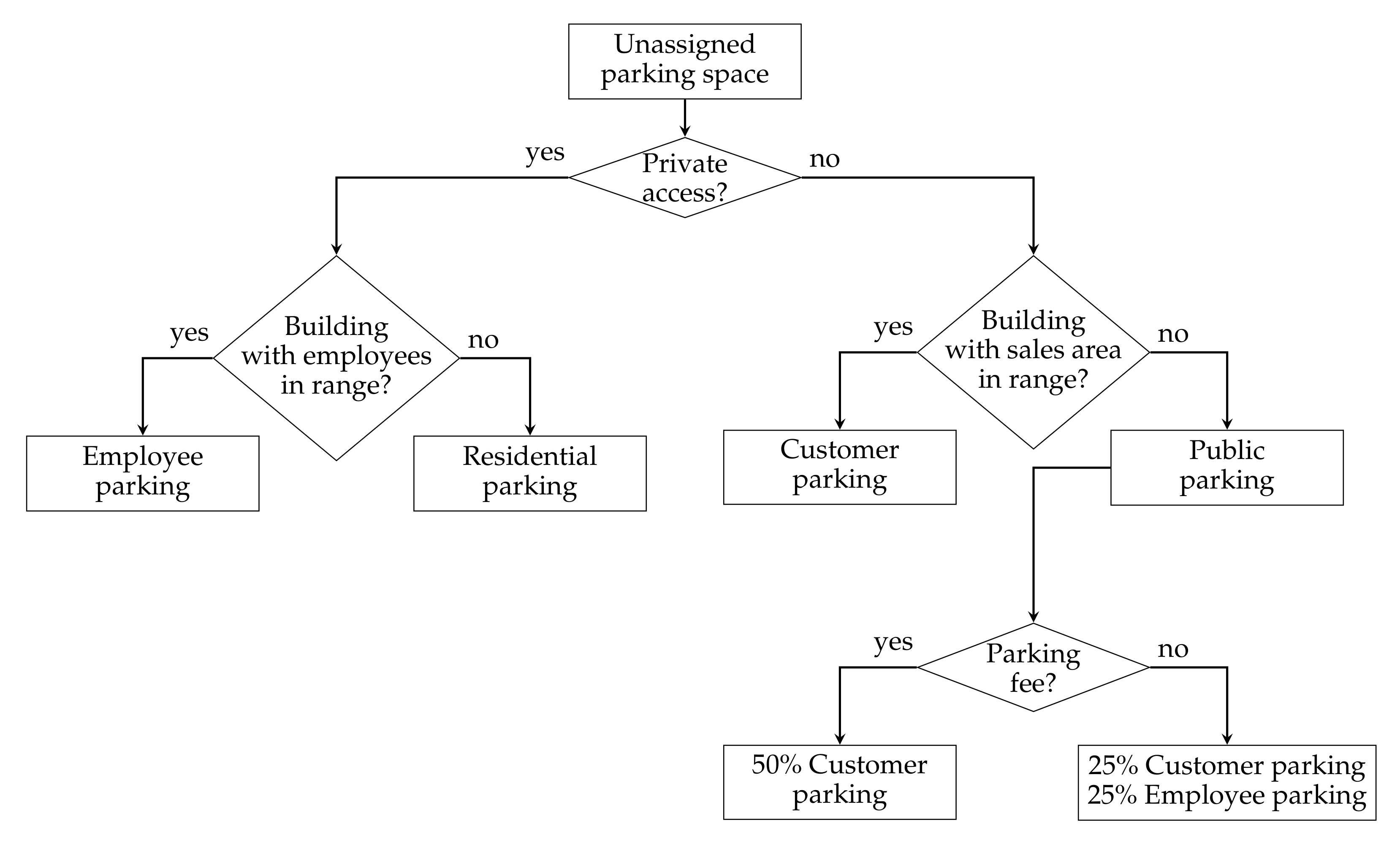
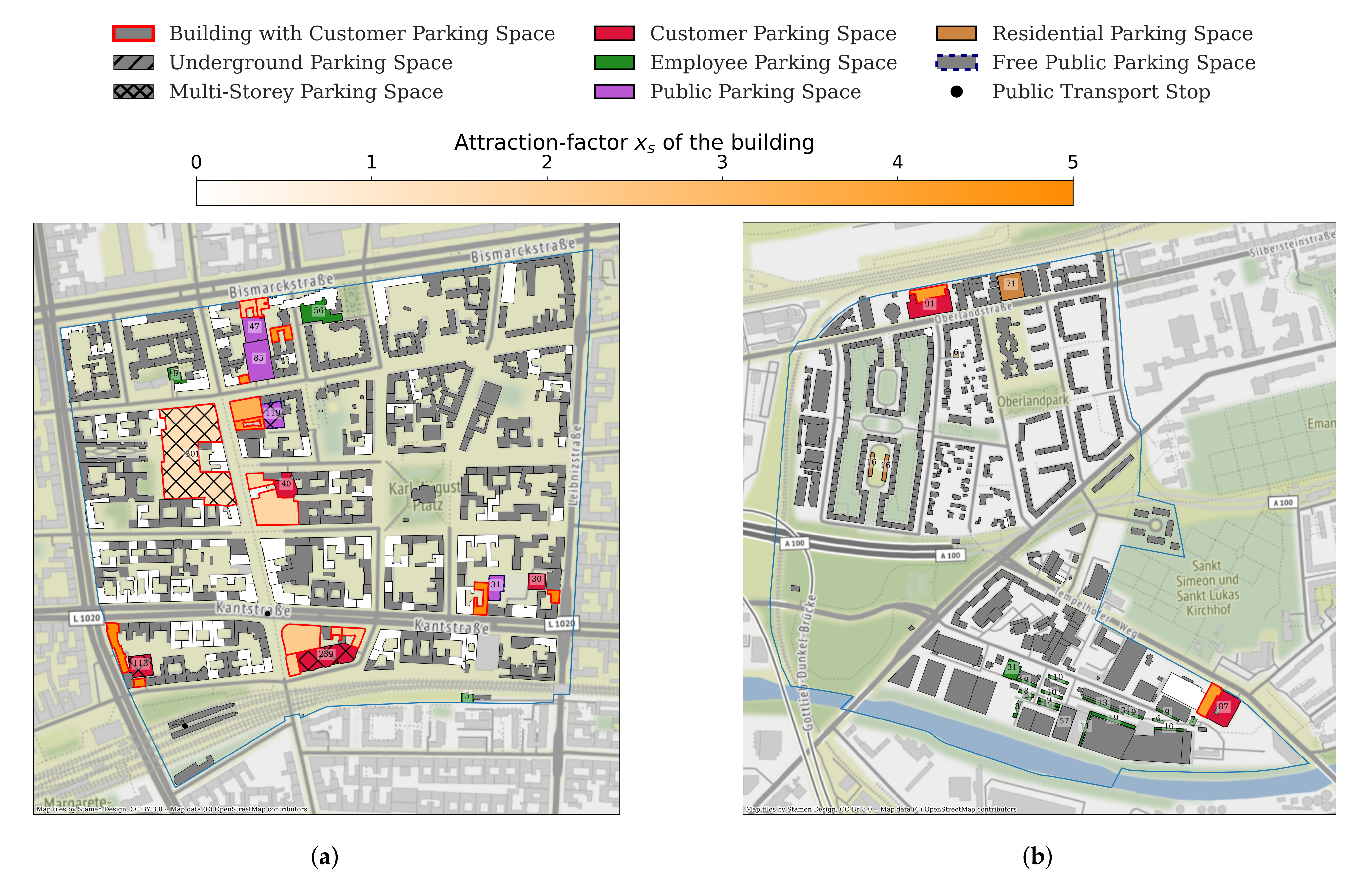
2.4. Parking Situation Analysis in the Berlin LORs

The goal of the parking situation analysis is to determine the number of parking spaces and their individual capacity within each LOR. The capacity of a parking space equals its number of parking spots. In addition, the intended use of the parking spaces is determined by the assignment of the parking spaces to one or more buildings. Since we aim to determine the attractiveness of the Berlin LORs for access by car for the activities working and shopping, this step is necessary to differentiate between employee, customer and other parking spaces.

For the analysis, we make use of the OSM data set which distinguishes between three different parking space classes that are suitable for cars.

• Surface parking spaces, which are single-level on the surface. Their gross parking area is equal to the surface area they cover, which can be directly derived from the OSM data set. The gross parking area includes areas for parking spots as well as areas that are part of the parking space but cannot be used for parking (e.g., columns or roads between parking spots).
• Multi-storey parking spaces such as parking garages. Their gross parking area equals the gross parking area per floor multiplied with the number of parking floors. The gross parking area per floor can be directly derived from the OSM data set, whereas the determination of the amount of parking floors is described in Section 2.1.
• Underground parking spaces, which are usually located beneath a building. Their gross parking area is calculated identically to that of multi-storey parking spaces. However, the OSM data set does not specify the gross parking area per floor as a percentage of the gross floor area of the building nor does it indicate the number of parking floors. Due to the high building density in Berlin and the resulting necessity for efficient use of construction space, we assume that the total gross floor area of the building is used for underground parking.

For each parking space class, there are parking spaces in the OSM data set for which their capacity is specified. In total, the capacity is known for 12.3% of the parking spaces. This allows easy back-calculation to parking spots per m${}^2$ of gross parking area. This correlation is shown in Figure 6, where each data point equals the given capacity information. By using linear regression, linear curves can be fitted to the data tuples. This relation can be used to determine the number of parking spots for parking spaces without capacity information. In order to confirm the applicability of this approach, we compared the number of parking spots estimated using the curves in Figure 6 with the correct number which was determined by manual counting for several parking spaces in all three parking space classes. The comparison showed reasonable deviations. In Figure 6, it can be seen that the curve for multi-storey parking spaces is steeper compared to the curve of surface parking spaces, which is due to the more efficient use of space. Since no information is provided on the number of parking floors for underground parking spaces, their capacities are normalized to one floor. This results in an underestimation of gross parking area. The curve is therefore steeper compared to surface and multi-storey parking spaces since parking floors are implicitly included.

Since the number of parking spots of each parking space is known from the previous step, the usage class for each parking space needs to be determined through the assignment of the parking spaces to one or more buildings. The general assignment process is depicted in Figure 7 and is described below.

The access type for each parking space is given in the OSM data set. This information can be used to differentiate the parking spaces into four different usage classes: customer parking spaces (only accessible for shopping trips), private parking spaces for employee parking (accessible only for working trips), private parking spaces for residential parking (not accessible) and public parking spaces, which are accessible for shopping and working trips.

Parking spaces with private access need to be distinguished as parking spaces for employees or residential parking spaces. For this purpose, we consider all buildings that have a minimum distance of less than 50 m from the parking space (the influence of different distances on the result is investigated in Section 3.1 and Section 3.2) as potentially assignable to the parking space. If none of the potential buildings contains employees, the parking space is considered as a residential parking space. If one of the potential buildings contains employees, the parking space is assigned to this building and is considered as an employee parking space. If the parking space can be assigned to several buildings containing employees, the parking space is shared among those buildings according to their weighted number of employees, as expressed in Equation (6).

$$C_i=C_t·\frac{E_{bi}}{{\displaystyle \sum _{j=1}^m}{E}_{bj}}$$

(6)

where $C_t$ is the number of parking spots of the parking space, $C_i$ the number of the parking space’s spots assigned to the building i and $E_{bi}$ is the number of employees in building i, while m is the total number of buildings which are assigned to the parking space and their corresponding number of employees $E_{bj}$. If the access to the parking space is non-private, we check whether buildings exist that contain sales area and have a minimum distance of less than 10 m from the parking space. If one building meets these requirements, the parking space is assigned to this building as a customer parking space. If several buildings meet the requirements, the parking space is shared among those buildings according to their weighted sales area, as expressed in Equation (7).

$$C_i=C_t·\frac{S_{bi}}{{\displaystyle \sum _{j=1}^k}{S}_{bj}}$$

(7)

where $C_t$ is the capacity of the parking space, $C_i$ the amount of the parking space’s spots assigned to the building i and $S_{bi}$ is the sales area in building i, while k equals the total number of buildings which are assigned to the parking space and their corresponding sales area $S_{bj}$.

If no building meets the aforementioned requirements, the parking space is considered as a public parking space. The usage of public parking spaces varies greatly. Depending on their location and size, a different share of the parking space capacity is used for different activities. Therefore, it is difficult to make a general statement about their usage. We therefore assume that 50% of their capacity is used for activities which are not considered in this paper, such as leisure activities or doctor visits. For public charged parking, the remaining 50% of the parking space’s capacity is assigned to the buildings with sales area that have a minimum distance of less than 100 m from the parking space. The information on parking fees can be obtained directly from the OSM data set. The parking space’s spots are distributed among those buildings according to their weighted sales area (see Equation (7)). For free public parking spaces, we assign 25% of their capacity to buildings with sales areas and 25% to buildings with employees, according to their weighted sales area and number of employees. For this assignment we only consider buildings with sales area which have a minimum distance of less than 100 m from the parking space and buildings with employees which have a minimum distance of less than 200 m from the parking space (the influence of different distances on the result is investigated in Section 3.1 and Section 3.2).

2.5. Attractiveness-Based District Rating for Shopping Trips

In order to compute the attractiveness of districts to drive to by car for shopping trips, we use a two-step approach. In the first step, we determine the car-access attractiveness of the individual buildings in the LOR. In the second step, we aggregate the results at the LOR level to derive an overall rating for the district. In the literature, the attractiveness of shopping locations is typically represented by their amount of sales area [17,18]. The parking situation, which is crucial for the car-access attractiveness of shopping locations, is not considered. To overcome this limitation, in this paper, we determine the attractiveness of each building in the LORs by considering both the sales area and the overall availability of parking spots. To achieve this, we combine the following three criteria:

• Criterion $y_{1s}$: the amount of parking spots per m${}^2$ sales area.
• Van der Waerden et al. [37] as well as Zhang et al. [38] showed that persons prefer low walking distances between a parking facility and their final destination. Thus, as a second criterion, $y_{2s}$, we consider the distance of the parking space to the building.
• Hymel [39] and van der Waerden et al. [40] showed that when a shopping location charges for parking, the number of shopping trips there decreases. Therefore, the third criterion for car-access attractiveness evaluation $y_{3s}$ is whether parking fees have to be paid for the use of the parking space.

To determine the car-access attractiveness of a building from the three criteria, we apply the weighted sum model, which is typically used for multicriteria decision analysis [41]. The fundamental concept behind this technique is the additive utility assumption. If each criterion is measurable and has the same unit, then the best alternative is the one with the largest cumulative value [41,42]. The value P of each alternative j can be computed as

$$P_j=\sum _{i=1}^n{a}_i·w_i\mathrm{for}j=1,2,\dots ,m$$

(8)

where n is the number of criteria, $a_i$ is the value of the criterion i and $w_i$ is the individual weighting-coefficient of the criterion i. In principle, the higher the weighting, the more important the criterion. Normally, the weighting-coefficients are normalized so that they sum to one [41]. For the application of the weighted sum model, all criteria must have the same unit. For this purpose, we use the rating-coefficients ${\beta }_{1s}$, ${\beta }_{2s}$ and ${\beta }_{3s}$ that assign a discrete value between 1 (very unattractive) and 5 (very attractive) to value ranges of the criteria $y_{1s}$, $y_{2s}$ and $y_{3s}$. In

Table 3. Value ranges of the parking spots per m${}^2$ sales area $y_{1s}$, the building’s distance to the parking space $y_{2s}$, parking fees $y_{3s}$ and their corresponding rating.

Rating-	Parking Spots per m${}^2$	Distance to	Parking Fees
Coefficient	Sales Area ${\mathit{y}}_{1\mathit{s}}$	Parking Space ${\mathit{y}}_{2\mathit{s}}$	${\mathit{y}}_{3\mathit{s}}$
1 (very unattractive)	$y_{1s}\le 0.025$	$80m<y_{2s}\le 100m$	yes
2 (unattractive)	$0.025<y_{1s}\le 0.05$	$60m<y_{2s}\le 80m$	-
3 (medium)	$0.05<y_{1s}\le 0.075$	$40m<y_{2s}\le 60m$	-
4 (attractive)	$0.075<y_{1s}\le 0.1$	$20m<y_{2s}\le 40m$	-
5 (very attractive)	$y_{1s}>0.1$	$y_{2s}\le 20m$	no

, the value ranges of the criteria and their corresponding rating-coefficients are given. Since there is no parking space ordinance in Berlin that prescribes the number of parking spots for buildings with retail usage, the value ranges for $y_{1s}$ are derived in this paper by manually calculating the number of parking spots per m${}^2$ of sales area for fifteen “Aldi” supermarkets. “Aldi” supermarkets are chosen, as they can be regarded as “average” Berlin supermarkets (see Section 2.2). The computed average value of 0.1 parking spots per m${}^2$ sales area is considered as very attractive. Linear division is used to specify the remaining value ranges. As we described in Section 2.4, parking spaces can only be assigned to buildings with sales area to which they have a minimal distance of less than 100 m. Accordingly the value ranges of $y_{2s}$ are divided linearly. For the criterion parking fee $y_{3s}$, we do not consider ranges. We differentiate between free parking spaces which are very attractive and parking spaces with fees which are very unattractive. In Section 3.1, the influence of modified value ranges of the factors $y_{1s}$, $y_{2s}$ and $y_{3s}$ on the result is investigated.

For each building with sales area and assigned parking spaces, its car-access attractiveness, hereinafter called attraction-factor $x_s$, is computed as the weighted sum of the three aforementioned criteria according to Equation (9). It is possible that several parking spaces can be assigned to a building, each with a different distance to the building and different parking fees. Therefore, in order to receive a global rating-coefficient ${\beta }_{2s}$ and ${\beta }_{3s}$ for each building, the rating-coefficients of the parking spaces are weighted according to their number of parking spots assigned to the building.

$$\begin{array}{cc}\hfill & x_s=a_{1s}·w_{1s}+a_{2s}·w_{2s}+a_{3s}·w_{3s}\mathrm{with}\sum _{i=1}^3{w}_{is}=1\hfill \\ \hfill & a_{1s}={\beta }_{1s}\hfill \\ \hfill & a_{2s}=\frac{1}{C_{tb}}\sum _{i=1}^n{C}_{ib}·{\beta }_{i2s}\hfill \\ \hfill & a_{3s}=\frac{1}{C_{tb}}\sum _{i=1}^n{C}_{ib}·{\beta }_{i3s}\hfill \end{array}$$

(9)

In Equation (9), $C_{tb}$ is the total number of parking spots assigned to the building, n is the total number of parking spaces assigned to the building and $C_{ib}$ is the number of parking spots of the parking space i. $w_{1s}$, $w_{2s}$ and $w_{3s}$ are the weighting-coefficients of the criteria. Their values can range from 0 to 1, and their sum equals 1. Hence, the attraction-factor $x_s$ of the building can take continuous values between 1 and 5. Buildings with sales area that have not been assigned a parking space receive an attraction-factor $x_s$ of 0.

Since the attraction-factor $x_s$ of each building is known, the total LOR attractiveness $A_s$ for shopping trips by car can be calculated by weighting each building by its sales area according to Equation (10).

$$A_s=\frac{1}{S_t}\sum _{i=1}^m{S}_{bi}·x_{is}$$

(10)

In Equation (10), $S_t$ is the total number of sales areas in the LOR, m is the total number of buildings with sales area in the LOR and $S_{bi}$ is the sales area of the building i. Since the attraction-factor $x_s$ can take values between 0 and 5, the attractiveness $A_s$ of the LOR can take continuous values between 0 and 5 as well. A high car-access attractiveness $A_s$ means that an LOR is highly likely to be accessed by car for a shopping activity, while low attractiveness means that people who shop at the LOR are more likely to choose another mode of transportation to travel there.

2.6. Attractiveness-Based District Rating for Working Trips

In order to compute the attractiveness of districts to drive to by car for working trips, we use the same two-step approach as for the attractiveness-based district rating for shopping trips. In the literature, the attractiveness of working locations is typically represented by its number of employees [19]. We describe the car-access attractiveness of the buildings with employees by combining three criteria related to the parking situation.

• Criterion $y_{1w}$: the parking spots per employee.
• Criterion $y_{2w}$: the distance of the parking space to the building [37,38].
• Boulange et al. [43] and Limtanakool et al. [44] showed that short distances to public transportation services encourage public transport use. Therefore, the third criterion $y_{3w}$ is the average distance of the building to the nearest public transportation stop.

To apply the weighted sum model, all criteria must have the same unit. Therefore, we use the rating-coefficients ${\beta }_{1w}$, ${\beta }_{2w}$ and ${\beta }_{3w}$ that assign a discrete value between 1 and 5 to the value ranges of the criteria $y_{1w}$, $y_{2w}$ and $y_{3w}$. This relationship is shown in

Table 4. Value ranges of the parking spots per employee $y_{1w}$, the building’s distance to the parking space $y_{2w}$ and public transport stop $y_{3w}$ and their corresponding rating.

Rating-Coefficient	Parking Spots per Employee ${\mathit{y}}_{1\mathit{w}}$	Distance to Parking Space ${\mathit{y}}_{2\mathit{w}}$	Distance to Public Transport Stop ${\mathit{y}}_{3\mathit{w}}$
1 (very unattractive)	$y_{1w}\le 0.01\overline{6}$	$160m<y_{2w}\le 200m$	$y_{3w}<200m$
2 (unattractive)	$0.0\overline{3}<y_{1w}\le 0.01\overline{6}$	$120m<y_{2w}\le 160m$	$200m\le y_{3w}<400m$
3 (medium)	$0.05<y_{1w}\le 0.0\overline{3}$	$80m<y_{2w}\le 120m$	$400m\le y_{3w}<600m$
4 (attractive)	$0.0\overline{6}<y_{1w}\le 0.05$	$40m<y_{2w}\le 80m$	$600m\le y_{3w}<800m$
5 (very attractive)	$y_{1w}>0.0\overline{6}$	$y_{2w}\le 40m$	$y_{3w}\ge 800m$

.

In the city of Berlin, there is no parking space ordinance that prescribes the number of parking spots for buildings with commercial usage. Therefore, the value ranges of $y_{1w}$ are derived by manually calculating the number of parking spots per employee for 15 companies with 250+ employees. The computed average value of $0.0\overline{6}$ parking spots per employees is considered as very attractive. Linear division is used to specify the remaining value ranges. As we described in Section 2.4, parking spaces can only be assigned to buildings to which they have a minimal distance of less than 200 m. Accordingly, the value ranges for the criterion $y_{2w}$ are divided linearly.

According to Wibowo and Olszewski [45], a distance of 400 to 800 m can be considered as acceptable walking distance to the nearest public transportation stop. In the state of Zürich in Switzerland, a distance of 400 to 750 m is considered as acceptable walking distance according to Schäffeler [46]. For the city of London, [47] considered 960 m as the maximum acceptable walking distance for rail, underground and light rail services. For Sydney, Daniels and Mulley [48] showed that people walk on average 573 m to a public transportation stop. In accordance with these findings, the value ranges of the criterion $y_{3w}$ are divided linearly. A walking distance of less than 200 m is considered as very unattractive, and a walking distance greater than 800 m is considered as very attractive to undertake the trip by car. Since the computation time to compute the average air distance between a building and its nearest public transportation stop is much faster compared to the computation of a walking distance, we introduce a general conversion factor of 1.494 ≈ 1.5, which means that 100 m of air distance equals 150 m of walking distance in the city of Berlin. This factor is determined by using the OpenRouteService Distance Matrix API [49] to compute the walking distance between two coordinates. For a data set containing 50,000 randomly distributed coordinates on Berlin roads (motorways, forests and parks are excluded), the conversion factor for all coordinate pairs with a walking distance of less than one kilometre is computed. The average result is used as a general conversion factor. In Figure 8, the average walking distance of the district buildings to the nearest public transportation is depicted for the district “Mitte”, which is located in the centre of Berlin, and the peripheral district “Spandau” in the west of Berlin. As expected, the comparison shows a high density of public transportation stops in the centre district “Mitte” and a low density in the peripheral district “Spandau”.

For each building with employees that also has assigned parking spaces, its attraction-factor $x_w$ is computed as the weighted sum of the three aforementioned criteria according to Equation (11). Since several parking spaces can be assigned to a building, each with a different distance to the building, the rating-coefficients ${\beta }_{2w}$ of the parking spaces are weighted.

$$\begin{array}{cc}\hfill & x_w=a_{1w}·w_{1w}+a_{2w}·w_{2w}+a_{3w}·w_{3w}\mathrm{with}\sum _{i=1}^3{w}_{iw}=1\hfill \\ \hfill & a_{1w}={\beta }_{1w}\hfill \\ \hfill & a_{2w}=\frac{1}{C_{tb}}\sum _{i=1}^n{C}_{ib}·{\beta }_{i2w}\hfill \\ \hfill & a_{3w}={\beta }_{3w}\hfill \end{array}$$

(11)

In Equation (11), $C_{tb}$ is the total number of parking spots assigned to the building, n is the total number of parking spaces assigned to the building and $C_{ib}$ is the number of parking spots of the parking space i. $w_{1w}$, $w_{2w}$ and $w_{3w}$ are the weighting-coefficients of the criteria. Buildings with employees that have not been assigned a parking space receive an attraction-factor $x_w$ of 0.

Since the attraction-factor $x_w$ of each building is known, the total LOR attractiveness $A_w$ for working trips by car can be calculated by weighting each building by its number of employees.

$$A_w=\frac{1}{E_t}\sum _{i=1}^m{E}_{bi}·x_{iw}$$

(12)

In Equation (12), $E_t$ is the total number of employees in the LOR, m is the total number of buildings with employees in the LOR and $E_{bi}$ is the number of employees of the building i. As shown for shopping trips in Section 2.5, the attractiveness $A_w$ of the LOR can take continuous values between 0 and 5. While a high car-access attractiveness indicates that a LOR is highly likely to be accessed by car for a working activity, a low attractiveness $A_w$ means that people who work at the LOR are more likely to choose another mode of transportation to travel there.

3. Results and Discussion

This section is organized as follows: the results of the attractiveness-based district rating are presented for shopping trips in Section 3.1 and for working trips in Section 3.2. In Section 3.3, the limits of the developed model are discussed, as well as possible future steps to improve the accuracy.

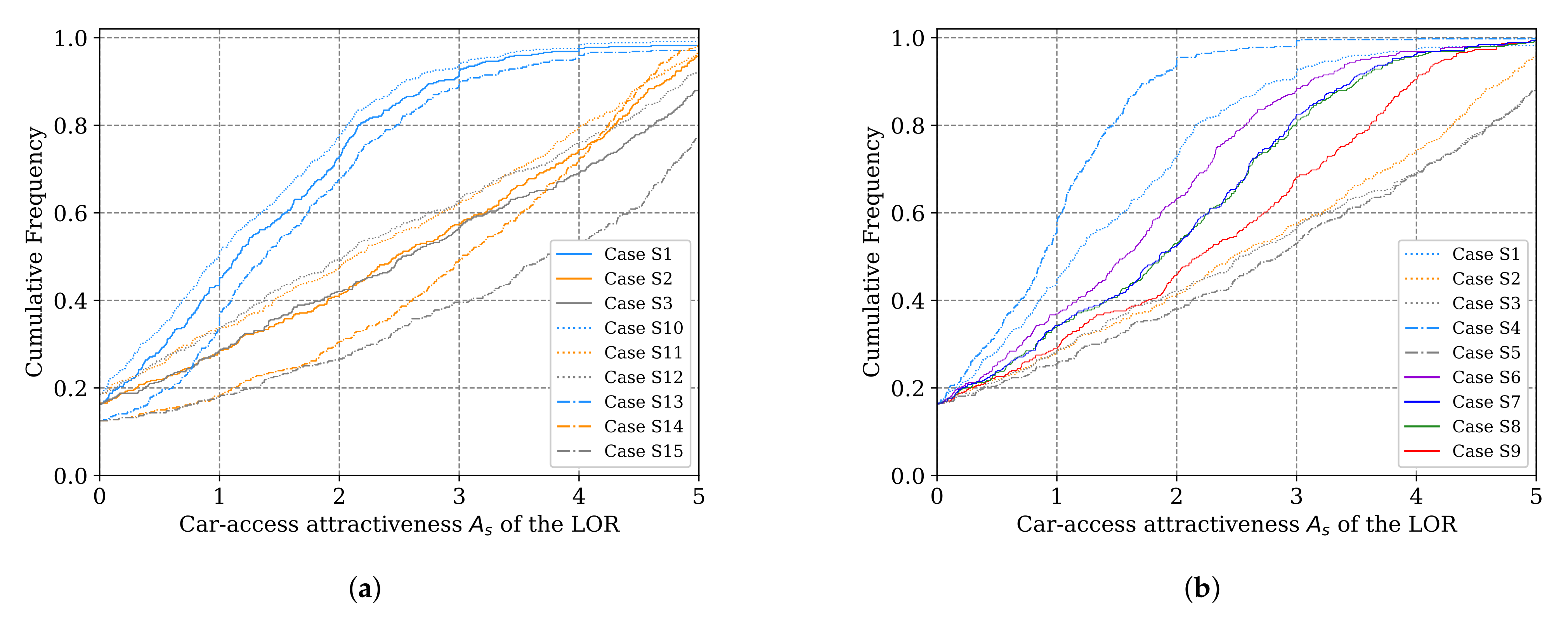
3.1. Attractiveness-Based District Rating for Shopping Trips

This section is divided into two parts. First, the results of the district rating are presented and discussed for the entire city of Berlin. Subsequently, the results for the buildings in two LORs are analysed.

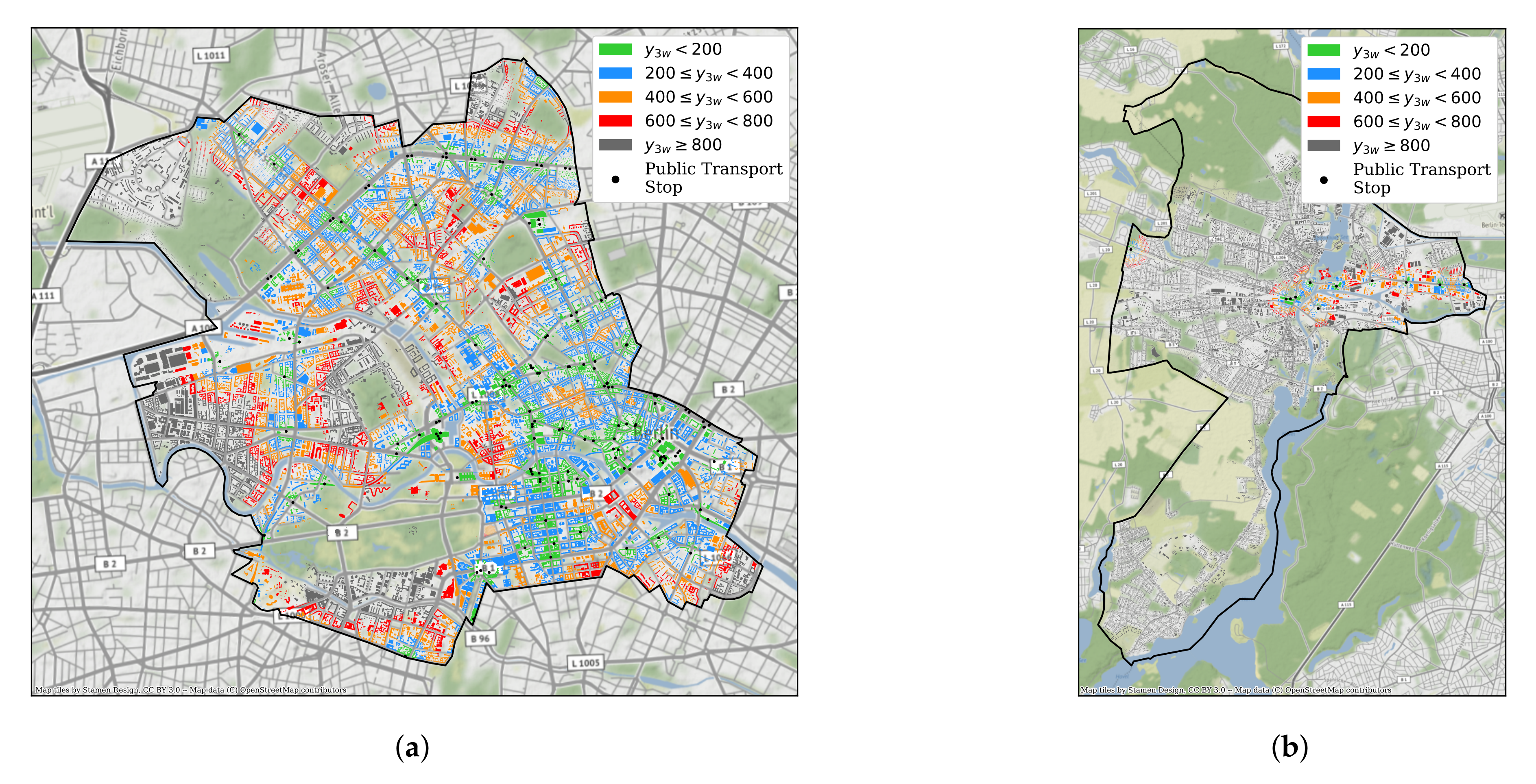
3.1.1. Results on Berlin Level for Shopping Trips

As we described in Section 2.5, the car-access attractiveness of the districts is computed by applying the weighted sum model. Depending on the choice of parameters, different results are obtained. Therefore, in this section, we conduct a sensitivity analysis based on 15 parameter combinations (hereafter referred to as cases) to assess the impact of different combinations on the car-access attractiveness of the LORs (see

Table 5. Investigated cases and selected parameters to compute the attractiveness of the Berlin LORs to drive to by car for shopping trips.

Cases	Weighting-Factors			Search Range Parking Space (m)			Parking Spots per m${}^2$ Sales Area		Distance to Parking Space ${\mathit{y}}_{2\mathit{s}}$		Parking Fees
	${\mathit{w}}_{1\mathit{s}}$	${\mathit{w}}_{2\mathit{s}}$	${\mathit{w}}_{3\mathit{s}}$	Employee	Public	Customer	Very Attractive	Very Unattractive	Very Attractive	Very Unattractive	No Fee	Fee
Case S1	1.0	0.0	0.0	50.0	100.0	10.0	$y_{1s}>0.1$	$y_{1s}\le 0.025$	$y_{2s}\le 20.0m$	$y_{2s}>80.0m$	very attractive	very unattractive
Case S2	0.0	1.0	0.0
Case S3	0.0	0.0	1.0
Case S4	1.0	0.0	0.0				$y_{1s}>0.2$	$y_{1s}\le 0.05$
Case S5	0.0	0.0	1.0				$y_{1s}>0.1$	$y_{1s}\le 0.025$			very attractive	medium
Case S6	0.8	0.1	0.1								very attractive	very unattractive
Case S7	0.6	0.3	0.1
Case S8	0.6	0.1	0.3
Case S9	0.3	0.3	0.3
Case S10	1.0	0.0	0.0		50.0	5.0			$y_{2s}\le 10.0m$	$y_{2s}>40.0m$
Case S11	0.0	1.0	0.0
Case S12	0.0	0.0	1.0
Case S13	1.0	0.0	0.0		300.0				$y_{2s}\le 60.0m$	$y_{2s}>240.0m$
Case S14	0.0	1.0	0.0
Case S15	0.0	0.0	1.0

). In the first step, the influence of the search range (i.e., the maximum distance between a parking space and the building it is assigned to) is analysed. In a further comparison, the influence of different value ranges of the criteria and different weighting-coefficients on the results is investigated.

In order to investigate the sensitivity of LOR attractiveness to search ranges, the cumulative distribution function of the car-access attractiveness $A_s$ of the LORs is depicted in Figure 9a for three different combinations of search ranges. For each combination, we also investigate the sensitivity of the LOR attractiveness to the criteria $y_{1s}$, $y_{2s}$ and $y_{3s}$ by successively setting the corresponding weighting-coefficient to 1 (as shown in Table 5). First, it can be seen that for each case investigated, the cumulative frequency is non-zero for $A_s=0$. This is due to the fact that there are LORs in which no parking space has been assigned to a building with sales area. In addition, there are LORs which do not contain buildings with sales areas, as in the case of forest, lake or industrial areas. As a result, those LORs receive an attractiveness $A_s$ of 0. It can be observed that the smaller the search ranges, the greater the number of LORs with a car-access attractiveness $A_s$ of 0, as simply fewer parking spaces are assigned to buildings.

The highest attractiveness ratings are obtained by the cases S3, S12 and S15 (grey), where only the criterion parking fee is considered, since the weighting-coefficient $w_{3s}$ is set to 1. The high rating is due to the fact that buildings that have been assigned one or more parking spaces without parking fees automatically receive an attraction factor $x_s$ of 5 (very attractive). However, this neglects the fact that only a very small number of parking spots may be assigned to the building or that the assigned parking spaces might be far away, since the weighting-coefficients $w_{1s}$ and $w_{2s}$ are set to 0. Good results are also obtained by cases S2, S11 and S14 (orange), where only the distance of the buildings from the parking spaces is considered to determine the attractiveness of the LORs. This is also mainly due to the fact that the number of parking spots is neglected. The lowest scores are achieved by cases S1, S10 and S13 (blue), where only the number of parking spots per m${}^2$ sales area is considered.

In order to investigate the sensitivity of LOR attractiveness to different value ranges of the criteria and different weighting-coefficients, the cumulative distribution function of car-access attractiveness $A_s$ is depicted in Figure 9b for a fixed search range. The comparison of case S1 and case S4 shows that when the threshold values of the criterion $y_{1s}$ (i.e., customer parking spots per sales area) are doubled, a significant decrease in LOR attractiveness $A_s$ is observed. This shows that the attractiveness rating is very sensitive to criterion $y_{1s}$. The car-access attractiveness rating is significantly less sensitive to a change in the parking fee criterion $y_{3s}$. This is shown by comparing cases S3 and S5, where it can be observed that the car-access attractiveness of the LORs increases only slightly when the threshold values of $y_{3s}$ are increased.

By comparing cases S6, S7, S8 and S9, the influence of different combinations of the weighting-coefficients on the results can be investigated. In accordance with the previous results, it can be seen that an increased weighting of the criterion $y_{1s}$ leads to a decreasing attractiveness of the LORs. Furthermore, the comparison of case S7 and case S8 shows that the influence of criteria $y_{2s}$ and $y_{3s}$ on the attractiveness of LORs is similar if the car-access attractiveness is determined using all three criteria.

In Figure 10, the spatial distribution of the car-access attractiveness $A_s$ of the Berlin LORs is shown for case S6 and is compared to the amount of sales area in the LORs. The parameter combination of case S6 is chosen because it results in medium attractiveness values for the entire city of Berlin (as shown in Figure 9b). The comparison of Figure 10a and Figure 10b shows that LORs with a high amount of sales area are mostly located in the city centre and do not match LORs with a high number of customer parking spaces per m${}^2$ of sales area, which are mostly located in the outer areas of the city. This is mainly due to the fact that the building density in the outer districts is low and therefore more space is available for parking. These results show that an attractiveness rating based only on total sales area is not an appropriate evaluation parameter to estimate the probability that a person will drive to a district for shopping by car, as the parking situation is neglected.

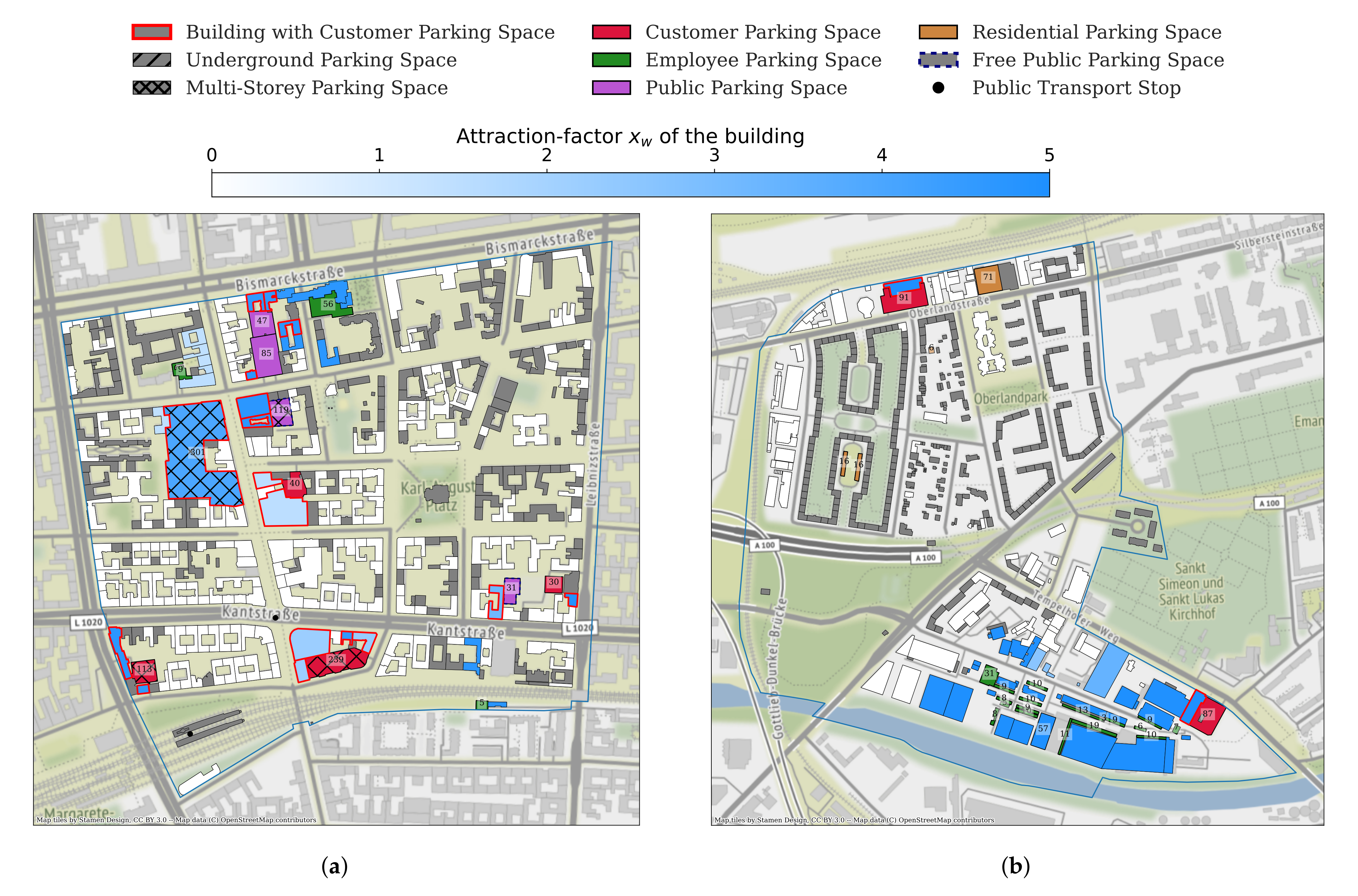
3.1.2. Results on LOR Level for Shopping Trips

For case S6, the results of the parking situation analysis and the attractiveness-based building rating are shown for two Berlin LORs in Figure 11. Buildings displayed in grey do not contain any sales area. Buildings displayed in white have an attraction-factor $x_s$ of 0 which means that no parking space has been assigned to these buildings. The numbers displayed on the parking spaces indicate the calculated number of parking spots. In case S6, the main weighting of car-access attractiveness is on the number of parking spots per m${}^2$ of sales area (weighting-coefficient $w_{1s}=0.8$). Accordingly, the buildings that have been assigned many parking spots receive a high attraction-factor. The average car-access attractiveness $A_s$ of the LOR “Karl-August-Platz” is 1.086. The average car-access attractiveness of the LOR “Germania Straße” is 1.772. The value for the “Germania Straße” is higher because a higher percentage of the buildings have been assigned parking spaces and thus do not receive an attraction-factor of 0. In addition, in the LOR “Karl-August-Platz”, several buildings often share one parking space. In contrast, in the “Germania Straße” LOR, customer parking spaces are each assigned to a single building, which then results in a higher number of parking spots per m${}^2$ of sales area.

3.2. Attractiveness-Based District Rating for Working Trips

The structure of this section is identical to Section 3.1. First, the results of the district rating for working trips are presented and discussed for the entire city of Berlin. Subsequently, the results for the buildings in two LORs are analysed.

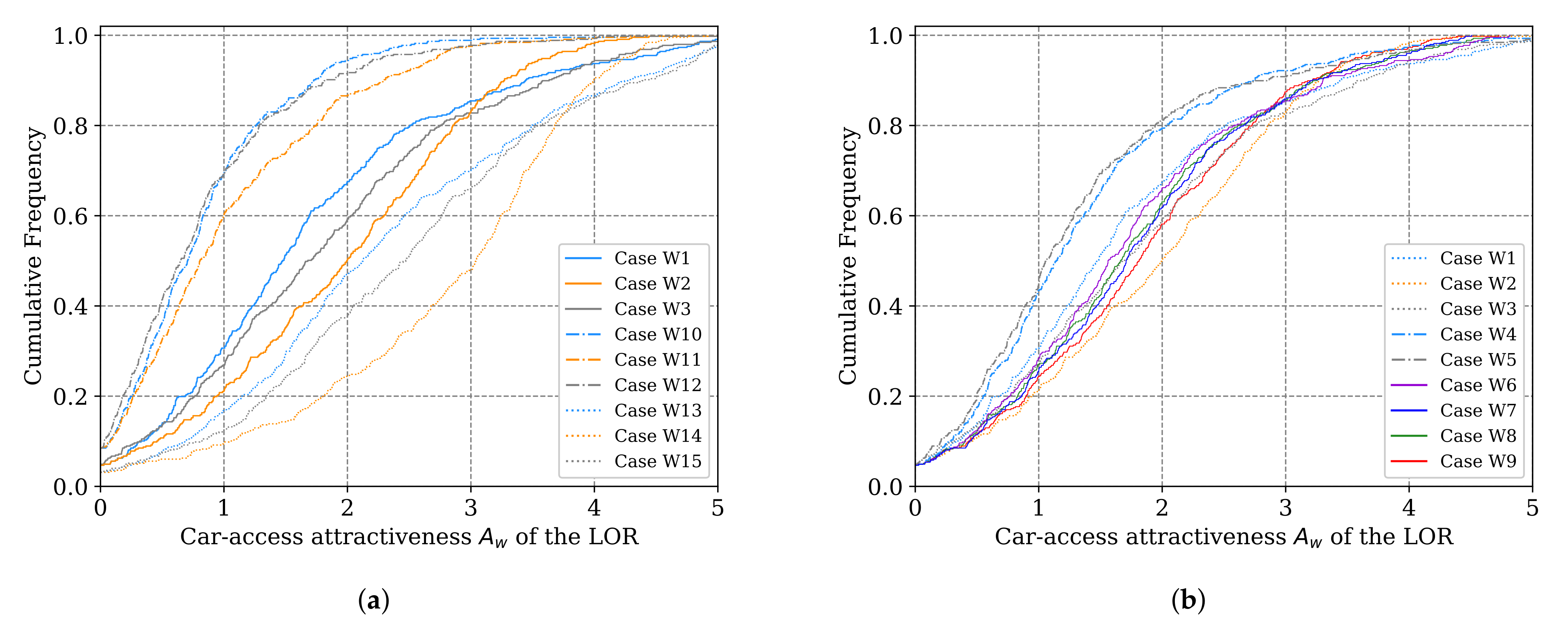
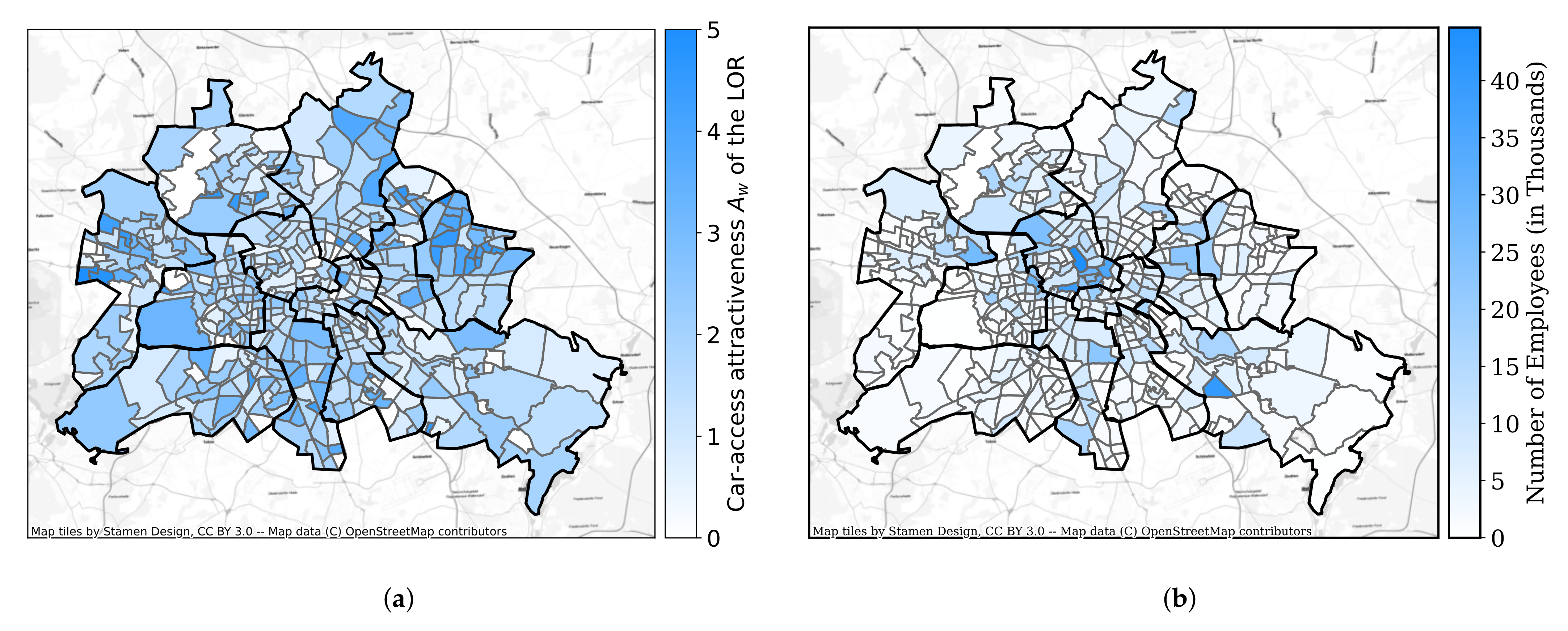
3.2.1. Results on Berlin Level for Working Trips

With the same objectives as in Section 3.1.1, a sensitivity analysis based on 15 parameter combinations is conducted in this section (see

Table 6. Investigated cases and selected parameters to compute the attractiveness of the Berlin LORs to drive to by car for working trips.

Cases	Weighting-Factor			Search Range Parking Space (m)			Parking Spots per Employee ${\mathit{w}}_{1\mathit{w}}$		Distance to Parking Space ${\mathit{y}}_{2\mathit{w}}$		Distance to Public Transport Stop ${\mathit{y}}_{3\mathit{w}}$
	${\mathit{w}}_{1\mathit{w}}$	${\mathit{w}}_{2\mathit{w}}$	${\mathit{w}}_{3\mathit{w}}$	Employee	Public	Customer	Very Attractive	Very Unattractive	Very Attractive	Very Unattractive	Very Attractive	Very Unattractive
Case W1	1.0	0.0	0.0	50.0	200.0	10.0	$y_{1w}>0.0\overline{6}$	$y_{1w}\le 0.01\overline{6}$	$y_{2w}\le 40.0m$	$y_{2w}>160.0m$	$y_{3w}\ge 800.0m$	$y_{3w}<200.0m$
Case W2	0.0	1.0	0.0
Case W3	0.0	0.0	1.0
Case W4	1.0	0.0	0.0				$y_{1w}>0.1\overline{3}$	$y_{1w}\le 0.0\overline{3}$
Case W5	0.0	0.0	1.0				$y_{1w}>0.0\overline{6}$	$y_{1w}\le 0.01\overline{6}$			$y_{3w}\ge 1600.0m$	$y_{3w}<400.0m$
Case W6	0.8	0.1	0.1								$y_{3w}\ge 800.0m$	$y_{3w}<200.0m$
Case W7	0.6	0.3	0.1
Case W8	0.6	0.1	0.3
Case W9	$0.\overline{3}$	$0.\overline{3}$	$0.\overline{3}$
Case W10	1.0	0.0	0.0	15.0	30.0	5.0			$y_{2w}\le 6.0m$	$y_{2w}>24.0m$
Case W11	0.0	1.0	0.0
Case W12	0.0	0.0	1.0
Case W13	1.0	0.0	0.0	150.0	400.0	10.0			$y_{2w}\le 80.0m$	$y_{2w}>320.0m$
Case W14	0.0	1.0	0.0
Case W15	0.0	0.0	1.0

).

For the investigation of the sensitivity of LOR attractiveness to search ranges, the cumulative distribution function of the car-access attractiveness $A_w$ is depicted in Figure 12a for three different combinations of search ranges. Additionally, the sensitivity of the LOR attractiveness to the criteria $y_{1w}$, $y_{2w}$ and $y_{3w}$ is investigated for each combination. It can be observed that for each case, the cumulative frequency is non-zero for $A_s=0$ and that smaller search ranges lead to a greater number of LORs with a car-access attractiveness $A_s=0$. These findings have already been justified in Section 3.1.1.

The highest attractiveness ratings are obtained by cases W2, W11 and W14 (orange), where only the distance of the buildings to the parking spaces is considered. This is because a building automatically receives a high attraction-factor $x_w$ if it is located near a parking space. However, this neglects that only a small number of parking spots may be assigned to the building. Intermediate results are obtained by cases W3, W12 and W15 (grey), where only the minimal distance of a building to the nearest public transportation stop is considered. The lowest scores are obtained by cases W1, W10 and W13 (blue), where only the number of parking spots per employee is considered.

For the investigation of the sensitivity of LOR attractiveness to different value ranges of the criteria and different weighting-coefficients, the cumulative distribution function of car-access attractiveness $A_w$ of the LORs is depicted in Figure 12b for a fixed search range. The comparison of case W3 and case W5 shows that the attractiveness rating is very sensitive to a change in the criterion distance to public transportation $y_{3w}$, since the doubling of its threshold values leads to a significant decrease in LOR attractiveness. This can be explained as follows: for case W5, an LOR attractiveness $A_w$ of 5 indicates that the distance of all buildings with employees to the nearest transportation stop is at least 1600 m. In Berlin, however, the public transport network is very well developed. Therefore, LORs in which all, or most, buildings meet these requirements are rare.

As observed for the district rating for shopping trips, the comparison of cases W6, W7, W8 and W9 shows that an increased weighting of the criterion $y_{1w}$ leads to a decreasing car-access attractiveness of the LORs, which is in accordance with the previous findings. In addition, the comparison of case W7 and case W8 shows that the influence of criteria $y_{2w}$ and $y_{3w}$ on the attractiveness of LORs is similar if the car-access attractiveness is determined using all three criteria.

In Figure 13, the spatial distribution of the car-access attractiveness $A_w$ of the Berlin LORs is shown for case W6 and is compared to the number of employees in the LORs. The parameter combination of case W6 is chosen because it results in medium attractiveness values for the entire city of Berlin (as shown in Figure 12b). By comparing Figure 13a,b, it can be observed that LORs with a high quantity of employees are mostly located in the city centre area and do not match LORs with a high number of parking spaces per employee, which are mostly located in the outer areas of the city. The reasons for this and the implications of the results have already been discussed in the analogous study for shopping trips (see Figure 10).

3.2.2. Results on LOR Level for Working Trips

For case W6, the results of the parking situation analysis and the attractiveness-based building rating are shown for the LORs ”Karl-August-Platz” and ”Germania Straße” in Figure 14. Buildings displayed in grey do not contain any employees. Buildings displayed in white have an attraction-factor $x_w$ of 0, which means that no parking space has been assigned to these buildings. Since the main weighting of the car-access attractiveness $A_w$ is on the number of parking spots per employee (weighting-coefficient $w_{1w}=0.8$), the buildings that have been assigned many parking spots receive a high attraction-factor. The average car-access attractiveness $A_w$ of the LOR “Karl-August-Platz” is 1.263. The average car-access attractiveness of the LOR “Germania Straße” is 2.057. The low value in the LOR “Karl-August-Platz” is due to the high percentage of buildings that have not been assigned a parking space and therefore receive an attraction-factor of 0. Additionally, in the LOR “Karl-August-Platz”, most parking spaces are customer and public parking spaces. In contrast, there are many employee parking spaces in the LOR “Germania Straße”. As a result, many buildings, especially in the south of the LOR, have a high attraction factor, resulting in a higher attractiveness $A_w$ of the LOR.

3.3. Discussion

After presenting the results of the attractiveness-based district rating and the method for determining it, a couple of aspects concerning the proposed approach should be discussed.

• The proposed method should be validated by extensive surveys of motorists about their location choice behaviour. From the parameter combinations presented in Section 3.1 and Section 3.2 for calculating the attractiveness-based district rating, the combination that most accurately describes reality can then be selected.
• The proposed computation of the building’s attraction-factors $x_s$ and $x_w$ is based on the combination of three different criteria, each of which should be understood as the initial point for further improvements. Due to the weighted sum approach, additional criteria can be easily added in order to further refine the results.

  1.

  It is conceivable to investigate the accessibility of the building by determining the distance of the building to a main road using the OpenRouteService Distance Matrix API [49].

  2.

  Since OSM is a community project, geographic data are collected on a voluntary basis. Therefore, not every parking space is labelled as such in the data set. Unlabelled parking spaces are mainly located on the roadside. Based on a district’s land area, road network, building density and degree of motorisation, it is possible to estimate the number of unmarked roadside parking spaces available for shopping and work activities. The density of the buildings can be derived from the results of the building usage analysis (Section 2.1). The road network can be extracted from the OSM data set. For Berlin, the degree of motorisation is given in [50].

  3.

  In order to evaluate the car-access attractiveness of the work locations, we consider, among other criteria, the accessibility of the locations by public transportation. The results can be further improved by considering pedestrian and bicycle accessibility. This accessibility could be evaluated, for example, by infrastructure per capita, as shown in [51].

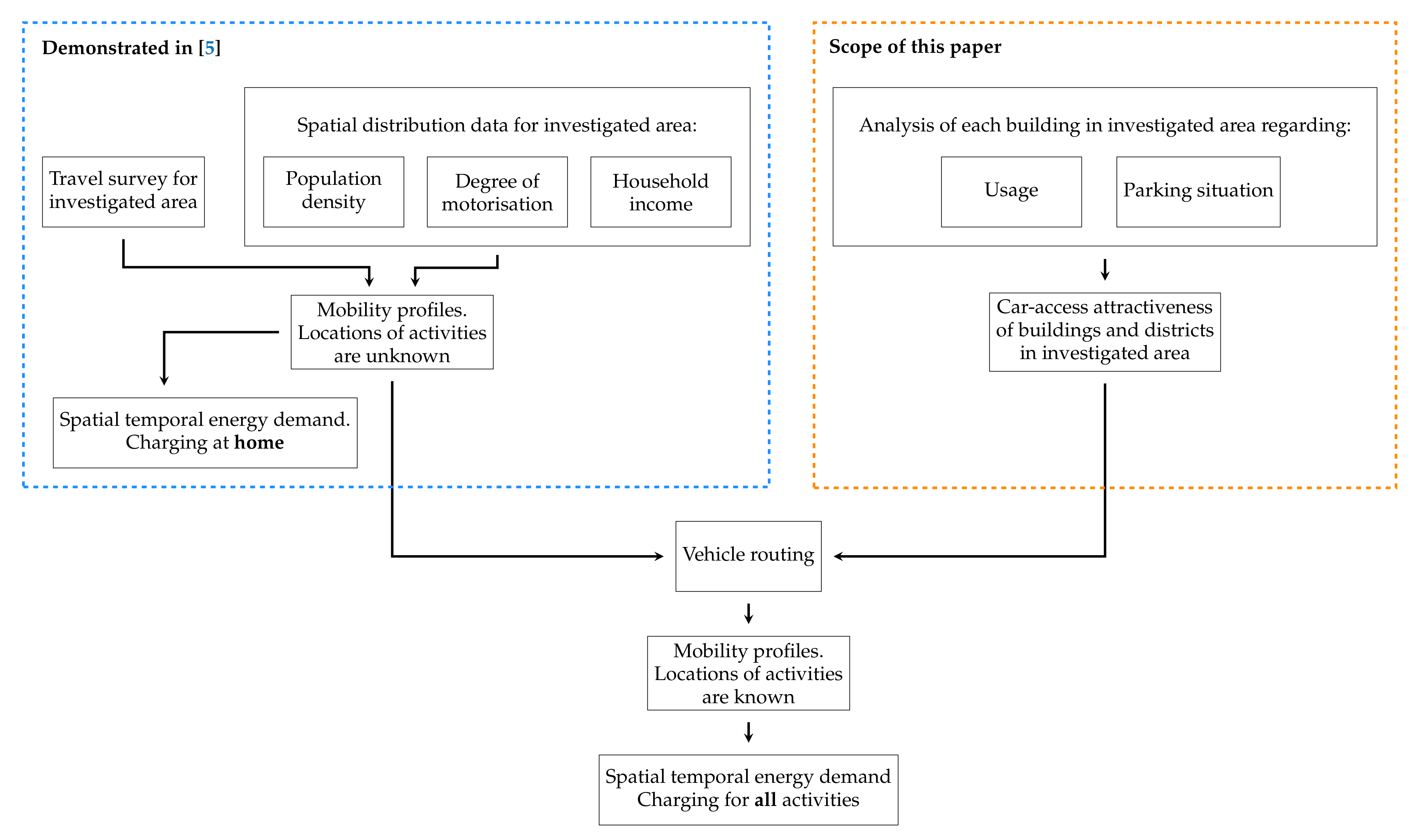
• As described in Figure 2, the vehicle-based mobility profiles and the attractiveness-based district rating can be combined with an appropriate routing algorithm to determine BEV routes. To avoid assigning too many BEVs to certain districts during the routing process, each district must be assigned a maximum intake capacity for each activity. One solution is to use the total number of customer or employee parking spots per district as an upper limit.

4. Conclusions and Outlook

The increasing number of battery electric vehicles (BEVs) and their demand for electrical power can lead to bottlenecks in the electrical grid infrastructure if it is not strengthened [3,4]. In order to locate those bottlenecks, the spatial distribution of the energy demand of BEVs needs to be known. For this purpose, travel schedules of individuals can be combined with an attractiveness rating of districts within an e-mobility traffic simulation to estimate traffic flows. Typically, attractiveness is represented by the “size” of locations (e.g., number of employees or sales area), assuming that larger places attract more persons than smaller ones [17,18,20]. Whereas this assumption can be applied when all modes of transportation are considered, it cannot be applied if cars are the only mode of transport under consideration, since the availability of parking spaces is neglected. Due to this neglect, department stores with a high amount of sales area and companies with many employees, for example, are classified as very attractive, regardless of whether sufficient parking infrastructure is available. Since the evaluation of car-access attractiveness of locations has not been addressed so far in the literature, this research gap is filled by this paper.

The car-access attractiveness of a district regarding shopping and working trips is determined in each case in a two-step process. First, we determine the car-access attractiveness of the individual buildings in the district by applying the weighted sum model and then aggregate the results on the district level. For shopping trips, the car-access attractiveness of a building is based on three criteria: the amount of parking spots per sales area of the building, the distance of the parking spaces to the building and whether there are fees for the usage of the parking spaces. For working trips, the car-access attractiveness is computed by considering the number of parking spots per employee of the building, the distance of the parking spaces to the building and the average distance of the building to the nearest public transportation stop. We have demonstrated the approach for the urban area of Berlin and its 448 sub-districts called LORs. Since the method is based on open geodata and freely available data sets, our approach is traceable and reproducible. The data sets we used to develop our method are available in a similar or identical form in many rural and urban regions in Germany. Therefore, an upscaling of our model is feasible. For Berlin, we show that LORs with a great amount of sales area or employees are mostly located in the city centre. Those LORs would obtain high attractiveness under the assumption that larger places are more attractive. However, this contradicts the fact that in Berlin, more parking spaces are available in the outer districts since the building density there is lower. In contrast, we showed that LORs with a high attractiveness according to our evaluation method are mostly located in the outer areas of the city, which matches the parking situation.

Our model provides an important building block for the complete evaluation of power demand due to the massive electrification of private urban mobility expected in upcoming years. Nevertheless, the validity of the model should be investigated in detail by surveying car drivers on their location choice behaviour in the near future.

References

1. Presse- und Informationsamt der Bundesregierung. Ziele der Bundesregierung: Bis 2030 die Treibhausgase Halbieren. 2019. Available online: https://www.bundesregierung.de/breg-de/themen/klimaschutz/klimaziele-und-sektoren-1669268 (accessed on 2 December 2020).
2. European Comission. The European Green Deal. 2019. Available online: https://eur-lex.europa.eu/legal-content/EN/TXT/?qid=1588580774040&uri=CELEX:52019DC0640 (accessed on 30 January 2021).
3. Lopes, J.A.P.; Soares, F.J.; Almeida, P.M.R. Integration of Electric Vehicles in the Electric Power System. Proc. IEEE 2011, 99, 168–183. [Google Scholar] [CrossRef] [Green Version]
4. Putrus, G.A.; Suwanapingkarl, P.; Johnston, D.; Bentley, E.C.; Narayana, M. Impact of electric vehicles on power distribution networks. In Proceedings of the VPPC ’09, Dearborn, MI, USA, 7–10 September 2009; IEEE: Piscataway, NJ, USA, 2009; pp. 827–831. [Google Scholar] [CrossRef]
5. Straub, F.; Streppel, S.; Göhlich, D. Methodology for Estimating the Spatial and Temporal Power Demand of Private Electric Vehicles for an Entire Urban Region Using Open Data. Energies 2021, 14, 2081. [Google Scholar] [CrossRef]
6. Knapen, L.; Kochan, B.; Bellemans, T.; Janssens, D.; Wets, G. Activity based models for countrywide electric vehicle power demand calculation. In Proceedings of the 2011 IEEE First International Workshop on Smart Grid Modeling and Simulation, Brussels, Belgium, 17 October 2011; pp. 13–18. [Google Scholar] [CrossRef] [Green Version]
7. Hidalgo, P.; Trippe, A.E.; Lienkamp, M.; Hamacher, T. Mobility Model for the Estimation of the Spatiotemporal Energy Demand of Battery Electric Vehicles in Singapore. In Proceedings of the 2015 IEEE 18th International Conference on Intelligent Transportation Systems (ITSC), Gran Canaria, Spain, 15–18 September 2015; pp. 578–583. [Google Scholar] [CrossRef]
8. Göhlich, D.; Nagel, K.; Syré, A.M.; Grahle, A.; Martins-Turner, K.; Ewert, R.; Miranda Jahn, R.; Jefferies, D. Integrated Approach for the Assessment of Strategies for the Decarbonization of Urban Traffic. Sustainability 2021, 13, 839. [Google Scholar] [CrossRef]
9. van Zuylen, H.J.; Willumsen, L.G. The most likely trip matrix estimated from traffic counts. Transp. Res. Part Methodol. 1980, 14, 281–293. [Google Scholar] [CrossRef]
10. Maher, M.J. Inferences on trip matrices from observations on link volumes: A Bayesian statistical approach. Transp. Res. Part Methodol. 1983, 17, 435–447. [Google Scholar] [CrossRef]
11. Savrasovs, M.; Pticina, I. Methodology of OD Matrix Estimation Based on Video Recordings and Traffic Counts. Procedia Eng. 2017, 178, 289–297. [Google Scholar] [CrossRef]
12. Bauer, D.; Richter, G.; Asamer, J.; Heilmann, B.; Lenz, G.; Kolbl, R. Quasi-Dynamic Estimation of OD Flows From Traffic Counts Without Prior OD Matrix. IEEE Trans. Intell. Transp. Syst. 2018, 19, 2025–2034. [Google Scholar] [CrossRef]
13. Alexander, L.; Jiang, S.; Murga, M.; González, M.C. Origin–destination trips by purpose and time of day inferred from mobile phone data. Transp. Res. Part Emerg. Technol. 2015, 58, 240–250. [Google Scholar] [CrossRef]
14. Iqbal, M.S.; Choudhury, C.F.; Wang, P.; González, M.C. Development of origin–destination matrices using mobile phone call data. Transp. Res. Part Emerg. Technol. 2014, 40, 63–74. [Google Scholar] [CrossRef] [Green Version]
15. Bachir, D.; Khodabandelou, G.; Gauthier, V.; El Yacoubi, M.; Puchinger, J. Inferring dynamic origin-destination flows by transport mode using mobile phone data. Transp. Res. Part Emerg. Technol. 2019, 101, 254–275. [Google Scholar] [CrossRef] [Green Version]
16. Ortúzar, J.d.D.; Willumsen, L.G. Modelling Transport, 4th ed.; Wiley: Chichester, UK, 2014. [Google Scholar]
17. Horni, A.; Scott, D.M.; Balmer, M.; Axhausen, K.W. Location Choice Modeling for Shopping and Leisure Activities with MATSim. Transp. Res. Rec. J. Transp. Res. Board 2009, 2135, 87–95. [Google Scholar] [CrossRef]
18. Kubis, A.; Hartmann, M. Analysis of Location of Large-area Shopping Centres. A Probabilistic Gravity Model for the Halle–Leipzig Area. Jahrb. Reg. 2007, 27, 43–57. [Google Scholar] [CrossRef]
19. Gonzalez-Feliu, J.; Peris-Pla, C. Impacts of retailing attractiveness on freight and shopping trip attraction rates. Res. Transp. Bus. Manag. 2017, 24, 49–58. [Google Scholar] [CrossRef]
20. Caceres, N.; Romero, L.M.; Benitez, F.G. Estimating Traffic Flow Profiles According to a Relative Attractiveness Factor. Procedia Soc. Behav. Sci. 2012, 54, 1115–1124. [Google Scholar] [CrossRef] [Green Version]
21. Drezner, T.; Drezner, Z. Validating the Gravity-Based Competitive Location Model Using Inferred Attractiveness. Ann. Oper. Res. 2002, 111, 227–237. [Google Scholar] [CrossRef]
22. Bömermann, H. Stadtgebiet und Gliederungen; Zeitschrift für amtliche Statistik: Berlin/Brandenburg, Germany, 2012; pp. 76–87. [Google Scholar]
23. Senatsverwaltung für Stadtentwicklung und Wohnen. Lebensweltlich Orientierte Räume (LOR) in Berlin: Planungsgrundlagen. 2021. Available online: https://www.stadtentwicklung.berlin.de/planen/basisdaten_stadtentwicklung/lor/ (accessed on 26 June 2021).
24. OpenStreetMap contributors. OpenStreetMap. 2021. Available online: https://www.openstreetmap.org (accessed on 4 February 2021).
25. Geofabrik GmbH. OpenStreetMap. 2021. Available online: https://www.geofabrik.de/en/geofabrik/ (accessed on 4 February 2021).
26. Open Knowledge Foundation. Open Data Commons: Open Data Commons Open Database License (ODbL). 2021. Available online: https://opendatacommons.org/licenses/odbl/ (accessed on 4 February 2021).
27. OpenStreetMap Wiki contributors. Elements. 2020. Available online: https://wiki.openstreetmap.org/w/index.php?title=Elements&oldid=2056268 (accessed on 4 February 2021).
28. Tillmann, H.G.; Kleiber, W.; Seitz, W. Tabellenhandbuch zur Ermittlung des Verkehrswerts und des Beleihungswerts von Grundstücken: Tabellen, Indizes, Formeln und Normen für die Praxis, 2nd ed.; Bundesanzeiger Verlag: Köln, Germany, 2017. [Google Scholar]
29. EHI Retail Institute GmbH. Entwicklung der Durchschnittlichen Verkaufsfläche der Lebensmittel-Discountmärkte Aldi Nord in Deutschland in den Jahren 2009 bis 2019 (in Quadratmetern). 2020. Available online: https://www.handelsdaten.de/lebensmittelhandel/durchschnittliche-verkaufsflaeche-discountmaerkte-aldi-nord-deutschland-zeitreihe (accessed on 7 February 2021).
30. EHI Retail Institute GmbH. Durchschnittliche Verkaufsfläche der Verkaufsstellen ausgewählter Lebensmittelhändler in Deutschland in den Jahren 2013 bis 2018 (in Quadratmetern). 2019. Available online: https://www.handelsdaten.de/lebensmittelhandel/durchschnittliche-verkaufsflaeche-der-standorte-ausgewaehlter (accessed on 7 February 2021).
31. Landesamt für Bauen und Verkehr. Einzelhandelsstruktur und Verkaufsflächen in der Hauptstadtregion Berlin-Brandenburg 2015/2016. 2017. Available online: https://lbv.brandenburg.de/dateien/stadt_wohnen/einzelhandelsstruktur_und_verkaufsraumfl_chen_in_der_hauptstadtregion_berlin-brandenburg_2015_2016.pdf (accessed on 27 June 2021).
32. Amt für Statistik Berlin-Brandenburg. Ergebnisse des Mikrozensus im Land Berlin 2016: Bevölkerung und Erwerbstätigkeit. 2017. Available online: https://www.statistik-berlin-brandenburg.de/publikationen/stat_berichte/2017/SB_A01-10-00_2016j01_BE.pdf (accessed on 7 February 2021).
33. Amt für Statistik Berlin-Brandenburg. Sozialversicherungspflichtig Beschäftigte im Land Berlin 30. Juni 2019. 2020. Available online: https://www.statistik-berlin-brandenburg.de/publikationen/Stat_Berichte/2020/SB_A06-20-00_2019j01_BE.pdf (accessed on 8 February 2021).
34. Fraunhofer-Institut für System- und Innovationsforschung. Energieverbrauch des Sektors Gewerbe, Handel, Dienstleistungen (GHD) in Deutschland für die Jahre 2011 bis 2013: Schlussbericht an das Bundesministerium für Wirtschaft und Energie (BMWi). 2015. Available online: https://www.bmwi.de/Redaktion/DE/Publikationen/Studien/sondererhebung-zur-nutzung-erneuerbarer-energien-im-gdh-sektor-2011-2013.pdf?__blob=publicationFile&v=6 (accessed on 27 June 2021).
35. Amt für Statistik Berlin-Brandenburg. Ergebnisse des Mikrozensus im Land Berlin 2019: Bevölkerung und Erwerbstätigkeit. 2020. Available online: https://www.statistik-berlin-brandenburg.de/publikationen/stat_berichte/2020/SB_A01-10-00_2019j01_BE.pdf (accessed on 7 February 2021).
36. Bundesagentur für Arbeit. Pendlerverflechtungen der sozialversicherungspflichtig Beschäftigten nach Kreisen: Berlin, Stichtag 30. Juni 2019. 2020. Available online: https://statistik.arbeitsagentur.de/SiteGlobals/Forms/Suche/Einzelheftsuche_Formular.html?nn=20934&topic_f=beschaeftigung-sozbe-krpend (accessed on 8 February 2021).
37. Van der waerden, P.; Timmermans, H.; de Bruin-Verhoeven, M. Car drivers’ characteristics and the maximum walking distance between parking facility and final destination. J. Transp. Land Use 2013. [Google Scholar] [CrossRef] [Green Version]
38. Zhang, W.; Gao, F.; Sun, S.; Yu, Q.; Tang, J.; Liu, B. A Distribution Model for Shared Parking in Residential Zones that Considers the Utilization Rate and the Walking Distance. J. Adv. Transp. 2020, 2020, 1–11. [Google Scholar] [CrossRef]
39. Hymel, K. Do parking fees affect retail sales? Evidence from Starbucks. Econ. Transp. 2014, 3, 221–233. [Google Scholar] [CrossRef]
40. Van der Waerden, P.; Borgers, A.; Timmermans, H. Consumer Response to Introduction of Paid Parking at a Regional Shopping Center. Transp. Res. Rec. J. Transp. Res. Board 2009, 2118, 16–23. [Google Scholar] [CrossRef]
41. Triantaphyllou, E.; Baig, K. The Impact of Aggregating Benefit and Cost Criteria in Four MCDA Methods. IEEE Trans. Eng. Manag. 2005, 52, 213–226. [Google Scholar] [CrossRef]
42. Fishburn, P.C. Additive Utilities with Incomplete Product Sets: Application to Priorities and Assignments. Oper. Res. 1967, 15, 537–542. [Google Scholar] [CrossRef]
43. Boulange, C.; Gunn, L.; Giles-Corti, B.; Mavoa, S.; Pettit, C.; Badland, H. Examining associations between urban design attributes and transport mode choice for walking, cycling, public transport and private motor vehicle trips. J. Transp. Health 2017, 6, 155–166. [Google Scholar] [CrossRef]
44. Limtanakool, N.; Dijst, M.; Schwanen, T. The influence of socioeconomic characteristics, land use and travel time considerations on mode choice for medium- and longer-distance trips. J. Transp. Geogr. 2006, 14, 327–341. [Google Scholar] [CrossRef]
45. Wibowo, S.S.; Olszewski, P. Modeling walking accessibility to public transport terminals: Case study of Singapore mass rapid transit. J. East. Asia Soc. Transp. Stud. 2005, 6, 147–156. [Google Scholar] [CrossRef]
46. Schäffeler, U. Netzgestaltungsgrundsätze für den öffentlichen Personennahverkehr in Verdichtungsräumen. Ph.D. Thesis, ETH, Zurich, Switzerland, 2005. [Google Scholar] [CrossRef]
47. Transport for London. Assessing Transport Connectivity in London. 2015. Available online: https://content.tfl.gov.uk/connectivity-assessment-guide.pdf (accessed on 23 February 2021).
48. Daniels, R.; Mulley, C. Explaining walking distance to public transport: The dominance of public transport supply. J. Transp. Land Use 2013, 6, 5. [Google Scholar] [CrossRef]
49. HeiGIT gGmbH. OpenRouteService: Services, Time-Distance Matrix. 2020. Available online: https://openrouteservice.org/services/ (accessed on 25 February 2021).
50. Senatsverwaltung für Umwelt, Verkehr und Klimaschutz. Mobilität der Stadt: Berliner Verkehr in Zahlen 2017. 2017. Available online: https://www.berlin.de/sen/uvk/verkehr/verkehrsdaten/zahlen-und-fakten/mobilitaet-der-stadt-berliner-verkehr-in-zahlen-2017/ (accessed on 2 September 2021).
51. Dingil, A.E.; Schweizer, J.; Rupi, F.; Stasiskiene, Z. Transport indicator analysis and comparison of 151 urban areas, based on open source data. Eur. Transp. Res. Rev. 2018, 10, 58. [Google Scholar] [CrossRef] [Green Version]
52. Verlag Der Tagesspiegel GmbH. Lückenschluss in der Fußgängerzone. 2007. Available online: https://www.tagesspiegel.de/berlin/lueckenschluss-in-der-fussgaengerzone/1052184.html (accessed on 20 March 2021).
53. IZ Immobilien Zeitung Verlagsgesellschaft mbH. Spandau Arcaden vor der Eröffnung. 2001. Available online: https://www.immobilien-zeitung.de/20401/spandau-arcaden-vor-eroeffnung (accessed on 20 March 2021).
54. BerlinOnline Stadtportal GmbH & Co. KG. Bikini Berlin. 2020. Available online: https://www.berlin.de/special/shopping/einkaufscenter/3305576-1724954-bikini-berlin.html (accessed on 20 March 2021).
Figure 1. Example of a general mobility profile.
Sustainability 13 11345 g001
Figure 2. Method for estimating the spatial and temporal energy and power demand from the electrification of private ICEVs.
Sustainability 13 11345 g002
Figure 3. Method for the attractiveness-based district rating for shopping and working trips.
Sustainability 13 11345 g003
Figure 4. Computed sales area per building for two Berlin LORs. (a) “Emdener Straße” LOR. (b) “Karl-August-Platz” LOR.
Sustainability 13 11345 g004
Figure 5. Computed number of employees per building for two Berlin LORs. (a) “Emdener Straße” LOR. (b) “Germaniagarten” LOR.
Sustainability 13 11345 g005
Figure 6. Linear approximation of the amount of parking spots per m 2 gross parking area from OSM data.
Sustainability 13 11345 g006
Figure 7. General process for the utilization assignment of parking spaces.
Sustainability 13 11345 g007
Figure 8. Average distance to the nearest public transportation stop y 3 w in the districts “Mitte” and “Spandau”. (a) District “Mitte”. (b) District “Spandau”.
Sustainability 13 11345 g008
Figure 9. Attractiveness-based district rating for shopping trips in the Berlin LORs. Cumulative distribution function. (a) Variable search range for parking spaces. (b) Constant search range for parking spaces.
Sustainability 13 11345 g009
Figure 10. Attractiveness-based district rating for shopping trips (case S6) and sales area in the Berlin LORs. (a) Case S6. (b) Sales area.
Sustainability 13 11345 g010
Figure 11. Attractiveness-based building rating for shopping trips for two Berlin LORs. Case S6. (a) “Karl-August-Platz” LOR. (b) “Germania Straße” LOR.
Sustainability 13 11345 g011
Figure 12. Attractiveness-based district rating for working trips in the Berlin LORs. Cumulative distribution function. (a) Variable search range for parking spaces. (b) Constant search range for parking spaces.
Sustainability 13 11345 g012
Figure 13. Attractiveness-based district rating for working trips (case W6) and number of employees in the Berlin LORs. (a) Case W6. (b) Number of Employees.
Sustainability 13 11345 g013
Figure 14. Attractiveness-based building rating for working trips for two Berlin LORs. Case W6. (a) “Karl-August-Platz” LOR. (b) “Germania Straße” LOR.
Sustainability 13 11345 g014