A Multi-Objective Meta-Heuristic Approach to Improve the Bus Transit Network: A Case Study of Fargo-Moorhead Area

Abstract

In this study, the Transit Network Design Problem (TNDP) is studied to determine the set of routes and frequency on each route for public transportation systems. To ensure the important concerns of planners like route length, route configuration, demand satisfaction, and attractiveness of the transit routes, the TNDP is solved to generate a set of routes by proposing an initial route set generation (IRSG) procedure embedded into the NSGA-II algorithm. The proposed IRSG algorithm aims to produce high-quality initial route set solutions to reach better optimization procedures. Moreover, the Multi-Objective Mixed-Integer Non-Linear Programming (MOMINLP) model is proposed to formulate the frequency setting problem on each route by minimizing the total travel time of passengers (user costs) and operator costs simultaneously, while maximizing the service coverage area near all the bus stops. The MOMINLP model is solved by applying the NSGA-II algorithm to produce a Pareto front between the first and the second objective functions. The model was applied to the Fargo-Moorhead Area (FMA), a small urban area. Results were compared with the existing transit network to measure the efficiency of the NSGA-II solution methodology. The proposed algorithm was found to considerably decrease the total travel time of passengers.

1. Introduction

Today, cities are growing faster than in the past in terms of population, congestion, and land use. Cities are experiencing challenges like worsening traffic congestion, increasing travel time, road accidents, insufficient public service, increasing pollution, etc. An optimally designed transit network is a crucial part of every urban transportation system that can help address many of these challenges. Transit is an effective service for supporting sustainable urban development. It also provides mobility options to transportation-disadvantaged populations not well served by other transportation options. Indeed, prioritizing transit is considered a strategy of urban development. However, while the transit network can have significant impacts on providing services to users and addressing urban transportation problems, services are costly to provide, and transit agencies have limited budgets. Transit agencies are tasked with attempting to satisfy multiple competing goals with a budget constraint. The Transit Network Design Problem (TNDP) model attempts to design an optimal transit network, given the constraints, that addresses many of the urban transportation problems while providing useful services to travelers and commuters. Several solutions have been addressed to solve the TNDP model.

The transit network consists of several connected routes, nodes, stations, and paths. Indeed, the TNDP is designed to consider multiple objectives including maximizing the number of travelers in the network [1,2], service coverage [3,4], demand density of the route including direct trips, one transfer, and two transfers [5], while also considering social and spatial equities [6]. It could also include objectives for minimizing total travel time, unsatisfied demand, total route length, the total number of routes taken by passengers, the total number of transfers, total user and operator cost, and total waiting time. The model includes natural constraints such as route length, number of stations, the distance between stations, bus frequency, the fleet size of vehicles, bus route, and travel demand in nature with different aspects of users and operators (see

Table A1. Literature Review.

References	Constraints	Objective Functions								Solution Methodology
		User Cost	Operator Cost	Travel Time	Unmet Demand	Fleet Size	Route Length	Waiting Time	Service Coverage
[12]	Timetable, Budget, Capacity, Assignment	✓	✓							Heuristic local search and scatter search algorithm
[13]	Headway feasibility, Load factor Fleet size, Trip length	✓	✓							Tabu search
[14]	Bus capacity, Frequency, Route length	✓	✓							Heuristic local search and scatter search algorithm
[15]	Demand Covering, Feasibility Constraints, Load factor, Fleet size, Travel time, Reliability		✓							Simulated annealing
[1]	Route feasibility			✓	✓					Genetic algorithm
[3]	Flow conservation, Route length, Service coverage, Range of subsidy						✓		✓	EUR—Constraint
[2]	The length of routes		✓							Parallel ant colony algorithm
[5]	Route length, Demand satisfaction, Route type									Ant colony optimization
[27]	Fleet size, minimum frequency setting			✓						Hybrid Genetic algorithm
[29]	Length of the transit route, Service frequency	✓			✓					Memetic Algorithm
[30]	Route configuration, Service frequency	✓	✓							Hybrid Algorithm
[31]	Route length, Frequency, Vehicle fleet		✓	✓						Genetic Algorithm
[46]	Routes and frequencies							✓		CPLEX 12 MILP solver
Current paper	Route length and frequency, Route configuration, and demand satisfaction			✓	✓		✓		✓	NSGA-II Algorithm

in Appendix A).

The TNDP is intended to find a series of routes for metropolitan public transport networks that optimize riders’ and operators’ competing goals with their respective frequencies. The key problem is the road network data and demand between various points of the cities. Constraints are typically linked to demand fulfillment, service level, and the availability of services, although additional constraints can occur. Frequencies are used in the optimization models of the transportation network, as they also have a significant effect on riders’ and operators’ cost structure.

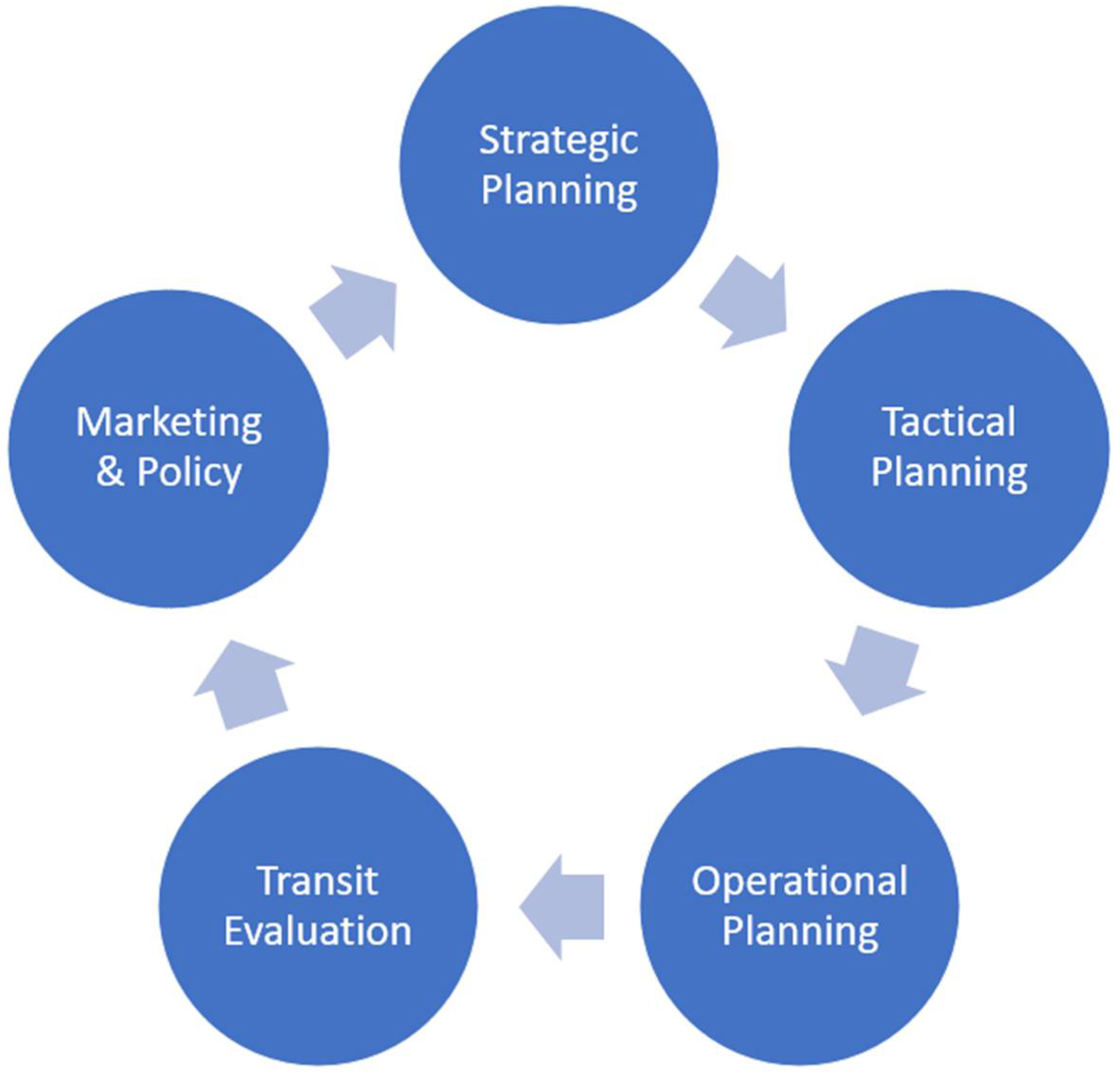
Transportation planning is embodied by five processes, including network design, frequency setting, timetable development, bus schedules, and driver scheduling [7]. In this study, the first two processes, network design and frequency setting, are addressed. Figure 1 displays these five plans in a schematic view. In another viewpoint, transportation planning can be divided into strategic planning (network design), tactical planning (frequency setting, timetable), and operational planning (bus scheduling and driver scheduling) [8]. The network design and frequency setting are components of long-term planning, which aims to create a balance between different objective functions such as minimizing passenger and operator costs [9].

The initial stage for each urban transit system is the strategic planning problems. Indeed, it determines the network layouts and some operational features. The goal is to optimize service quality within budget limits or to keep the cost for operators and users as low as possible [8]. Transferring transit design to a transport service requires tactical planning that links passengers with operators. The focus of tactical problems is to decide on public service delivery, in particular service frequencies along routes and timetables that can maximize service quality [10,11]. Operational planning addresses the problems of offering the proposed service at the lowest cost. This topic addresses various issues such as the planning and management of rolling stock, driver planning, scheduling of rolling stock, and maintenance. Transit network assessment is a way to receive passenger and operator feedback from the received service. It also shows where operators can improve service. Total transport accessibility, network reliability, and timing stability are part of the assessment for every transit network. Research on marketing strategies such as fare policies, investment strategies, and trade agreements as well as cooperation with other modes of transport is essential to the development of efficient transit systems which enhance their benefit for society and its residents.

Transit research often focuses on larger urban areas, but small urban systems face similar challenges. Further, because of lower population density and more dispersed demand, these systems face additional challenges in providing a high-quality service, without excessive travel times, that attracts riders and meets the needs of the public, while facing budget constraints. Therefore, this research focuses on the transit network in a small urban metropolitan area consisting of the cities of Fargo, North Dakota, and Moorhead, Minnesota, in the Midwest region of the United States.

In this study, a set of transit routes are designed in the existing Fargo-Moorhead Area (FMA) network. The bus route network is designed to improve the existing routes with predetermined bus stops to achieve an efficient transit network, minimizing the total travel time of passengers (user costs) and the number of operating buses (operator costs), while maximizing the service coverage in the network. This study attempts to answer the following questions:

• How should the routes be arranged, or bus stops be located in the FMA transit network?
• How many transit routes should be considered in the FMA transit network?
• How much will the new transit routes decrease travel time and the number of required buses operating?
• How much percent service coverage can be achievable?
• What would be an optimal number of buses as well as optimum bus headway in each route by proposing the new set of transit routes?

The rest of the paper is organized as follows. The literature review is discussed in Section 2. In Section 3, the mathematical model formulation and problem statement is proposed. The solution methodology is presented in Section 4. In Section 5, the case study of the existing network of FMA is explained and analyzed. Results of the proposed Non-dominated Sorting Genetic Algorithm II (NSGA-II) solution methodology are provided and discussed in Section 6. Finally, conclusions and further research directions are presented in Section 7.

2. Literature Review

Previous studies have developed models to address the TNDP, considering different objectives and using different techniques. This review examines the optimization objectives and solution techniques used in these studies. Table A1 in Appendix A provides more details on these studies.

2.1. Optimization Objectives

Studies that have developed TNDP models have proposed various objective functions. For example, some studies have considered minimizing operator costs, transit user costs, car user costs, and external costs [12,13,14,15]. Other studies only considered travel time and unsatisfied demand minimization [1]. Maximizing service coverage and minimizing route length was proposed by Chen et al. [3]. Islam et al. [16] minimized the total in-vehicle time, the total waiting time of all served passengers, percentage of passengers that bear transfers, fleet size as the total number of buses, total route length, percentage of unsatisfied demand, and degree of route overlap.

Some studies considered the concept of direct and indirect transfer [1,2,5,16,17]. Passengers who are traveling from one point to another point usually prefer to use the direct route which has a minimum number of direct transfers. Yu et al. [5] addressed this problem by defining a penalty in their objective functions that would minimize the number of transfers. They proposed a mathematical model to maximize transit demand density, which included direct trips and indirect trips with one transfer and two transfers. Moreover, Yang et al. [2] presented a formulation to maximize the total number of direct travelers per unit length. For more information, Table A1 classifies the past studies that employed the various constraints, objective functions, and solution methodology.

2.2. Solution Technique

During the past decades, with the emergence of search algorithms, researchers could solve optimization problems in a reasonable time. These algorithms are classified as metaheuristic and heuristic algorithms and are applied in a wide area of optimization problems. The TNDP model is classified as an NP-hard problem [18,19] and a non-convex (even concave) optimization problem [20]. So, some researchers proposed the heuristic algorithm at various levels of complexity to optimize parameters such as route spacing, route length, etc. [9,21,22,23].

On the other hand, most studies have considered heuristic algorithms at various levels of sophistication [9,21,22,24,25,26,27]. For example, Chakroborty and Wivedi [1] applied a technique of developing “optimum” routes using genetic algorithms in a real-world network. Yu [17] proposed the coarse-grain parallel ant colony algorithm (CPACA) to solve the problem utilizing search activities that are modified according to the objective value, to effectively find a globally optimal solution. A new CPACA algorithm was proposed by Yang et al. [2] to create a new technique for updating an increased pheromone called ant-weight, which adapts the path search behavior of ants to the objective purpose, and to use ant-colony algorithm parallelization (ACA) strategies to enhance time and efficiency of optimization. Fan and Machemehl [13] proposed the tabu search algorithm based on meta-heuristic algorithms. According to three variations of tabu search methods, they found the solution and tested it on a small network as a case study. A greedy algorithm was proposed by Careese and Gori [28] to determine the perfectly elastic demand for transit routes. Zhao et al. [29] used the Memetic algorithm (MA) to optimize the urban transit network. They considered four types of local search operators to improve the performance of the proposed algorithm. Buba and Lee [30] applied a Hybrid Differential Evolution-Particle Swarm Optimization (HDE-PSO) algorithm to configure the route as well as service frequency with multiple objectives simultaneously. Combining a genetic algorithm with agent-based travel demand modeling was proposed by Nnene et al. [31]. Finally, a heuristic-aided Stochastic Beam Search (SBS) algorithm was applied by Islam et al. [16] to provide a solution for the proposed TNDP model.

2.3. Research Gaps

Most of the research has studied minimization of user cost, operator cost, travel time, unsatisfied demand, and direct-undirect travelers [1,12,13,14,15,16,17]. Only a few studies have investigated the maximization of service coverage [17,32]. As an aspect of the solution, most studies employed the genetic algorithm in their solution methodology because of its wide applicability, such as [1,31]. Therefore, in this study, the NSGA-II algorithm is used to solve the proposed Multi-Objective Mixed-Integer Non-Linear Programming (MOMINLP) model. Indeed, the NSGA-II algorithm is powerful, and it is not widely used by many researchers in this field.

This paper attempts to address some of the challenges faced when proposing the MOMINLP model while applying it to the case study of the FMA network. So, the main contributions are as follows:

• Proposing the MOMINLP model including maximizing the service coverage of each transit route, minimizing the total travel time of passengers, and minimizing the total number of required buses operating in the network.
• Combining the IRSG procedure with the NSGA-II algorithm to generate a set of valid transit routes.
• Applying the proposed MOMINLP model to the real-world case study of the FMA to improve the existing network; and
• Conducting sensitivity analysis on parameters of the proposed NSGA-II algorithm to provide some insightful information for decision makers.

3. Proposed Model

In this study, a MOMINLP model is proposed to find the total travel time of passengers on each route, the round-trip time of each route, the bus headway of each route, the optimal number of required buses, the loading factor of each route, and the length of each generated route in the network.

3.1. Problem Statement

The TNDP model is defined as a network constituted by an undirected graph $G=\left(N,R\right)$ with a finite number of nodes (N) representing a transportation network and several arcs (R). N is devoted to the set of nodes (bus stations and terminals) and R is the set of existing network arcs (street route/street segment and path) that connects each bus stop to the other. Each element of R corresponds to a pair (i, j) where i is the origin and j is the destination. Each O-D has pair (i, j) and d_ij is denoted by travel demand between point i and j, and t_ij is denoted by travel time needed for passengers to move from point i to j. The solution of the TNDP model is a set of transit routes $R=\{r_1,r_2,r_3,\dots ,r_m\}$ in the network.

T and D are defined as the set of travel time and passenger trips between the node i and j, as follows:

$$T=\{t_{ij}|i,j\in [1,2,\dots ,N]\}$$

(1)

$$D=\{d_{ij}|i,j\in [1,2,\dots ,N]\}$$

(2)

The input data in this study is comprised of various matrices such as the distance matrix, the O-D (demand) matrix, and the travel time matrix. Then, these data are used as input to the model to get solutions consisting of transit routes and frequency settings.

3.2. Mathematical Model

The MOMINLP problem aims to determine the set of transit routes and frequency setting for a public transit system that should be convenient from the viewpoints of both users and operators. The TNDP model generates a set of transit routes and the frequency of each route, which determines the number of buses assigned to each route, to maximize demand served and avoid congestion and longer waiting times. This study has some assumptions, as follows:

• The number of transit routes is determined by the planner.
• The frequency in each route should be within a range.
• Route length should be within a minimum and maximum range.
• The fleet size is considered as the budget constraint on each route.
• The bus headway is considered as a constraint to avoid longer passenger waiting time.

Moreover, the following criteria are used to produce high-quality transit routes:

• The route feasibility check verifies that no repeated vertices are displayed on a route, that each route is feasible.
• If a route is identical to one segment or an entire route, then this route will be considered non-unique. So, this route will be removed directly.
• The network connectivity check determines if a route is linked to the public transit system.
• The area coverage check verifies that all vertices are shown in a set solution at least once. This process builds a list of appearing vertexes by searching all routes and checking when each vertex is listed.

In this study, the MOMINLP model is proposed to minimize the total travel time of users and the number of buses simultaneously, as well as to maximize the service coverage (potential demands) of generated transit routes in the network. The following sub-sections describe the parameters, variables, and the mathematical model.

3.2.1. Parameters

To build the model, the following parameters are used:

• $D_{ij}^{TotNet}$: Total passenger demand on the network (persons)
• $L_{\min }^{r_m}$: The minimum length of laid route for the route r_m (meters)
• $L_{\max }^{r_m}$: The maximum length of laid route for the route r_m (meters)
• $S_{\min }$: The minimum space of station between two nearby stations of i and j (meters)
• $S_{\max }$: The maximum space of station between two nearby stations of i and j (meters)
• $W_1,W_2$: The penalty coefficient reflecting the importance of each term of first objective functions including the user costs and operator costs
• $B{H}_{\min }$: The minimum bus headway required for each route (minutes)
• $B{H}_{\max }$: The maximum bus headway required for each route (minutes)
• $B$: The maximum bus fleet size on the existing network (buses)
• $R_{\max }$: The maximum number of transit routes in the network
• $U_d$: The value of unmet demand ($/person)
• $V_t$: The value of time ($/minute)
• $O_v$: The operating hours for the bus running on any route (minutes)
• $L{F}_{\max }$: The maximum load factor for any route in the network (per bus)
• $S$: Seating capacity of each operating bus (persons)

3.2.2. Variables

Variables are defined as follows:

• $T{R}_{ij}^{r_m}$: The total travel time between stops i and stop j on route r_m
• $D_{ij}^{r_m}$: Total passenger demand between stop i and stop j along route r_m
• $R{T}_{r_m}$: The round-trip time of route r_m (minutes)
• $B{H}_{r_m}$: The bus headway operating on route r_m (minutes)
• $L^{r_m}$: The length of route r_m
• $DI{S}_{ij}$: The distance between the stop i and stop j on the network
• $N$: The number of routes of the newly designed transit network
• $F{S}_{r_m}$: The number of operating buses required on route r_m
• $L{F}_{r_m}$: The load factor of route r_m
• $Q_{\max }^{r_m}$: The maximum flow on route r_m

3.2.3. Objective Functions

From the mathematical point of view, the MOMINLP model can be expressed as follows:

$$Min{Z}_1=W_1({\displaystyle \sum _{i\in N}^{}{\displaystyle \sum _{j\in N}^{}{\displaystyle \sum _{r_m\in R}^{}{D}_{ij}^{r_m}}}}·T{R}_{ij}^{r_m})+W_2·O_v·({\displaystyle \sum _{r_m\in R}^{}\frac{R{T}^{r_m}}{B{H}^{r_m}}})$$

(3)

$$Max{Z}_2=\frac{{\displaystyle \sum _{i\in N}{\displaystyle \sum _{j\in N}{\displaystyle \sum _{i,j\in r_m}^{}{D}_{ij}^{r_m}}}}}{{\displaystyle \sum _{i\in N}^{}{\displaystyle \sum _{j\in N}^{}{D}_{ij}^{TotNet}}}}$$

(4)

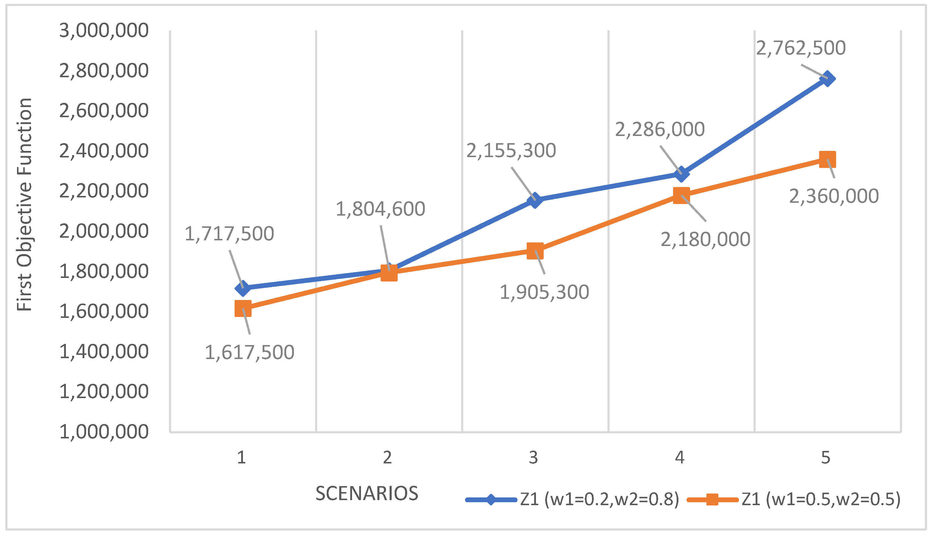
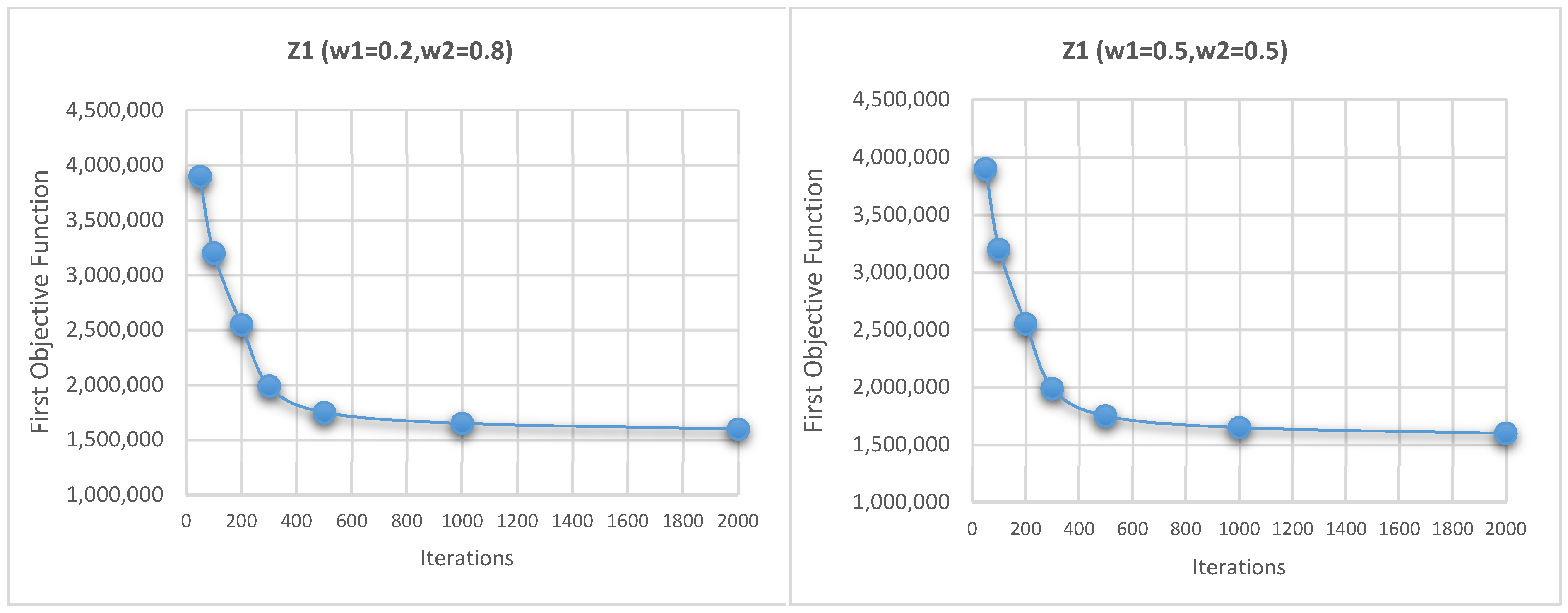
The first objective function shown by Equation (3) is constituted by two parts including user cost and operator cost. Generally, the user cost consists of four components such as walking time, waiting time, transfer time, and in-vehicle time (i.e., the in-vehicle time required for riding a bus to a destination), and the operator cost is the cost of operating buses. On the other hand, $W_1,W_2$ are penalty coefficients of these two parts that refer to the tradeoffs between the user costs and the operating costs. These coefficients are determined by decision-makers. Therefore, different rates of these coefficients result in a different set of optimal transit routes.

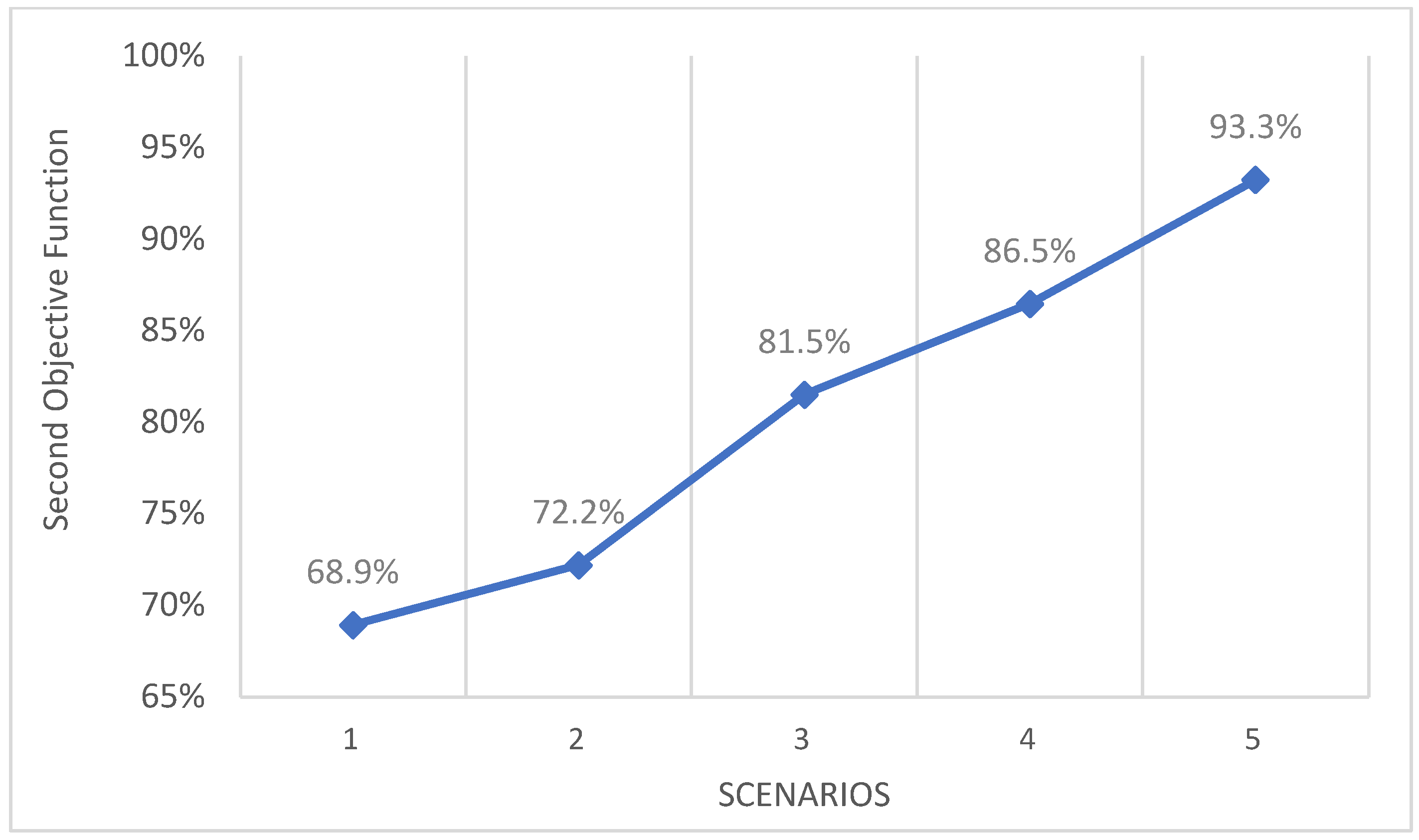
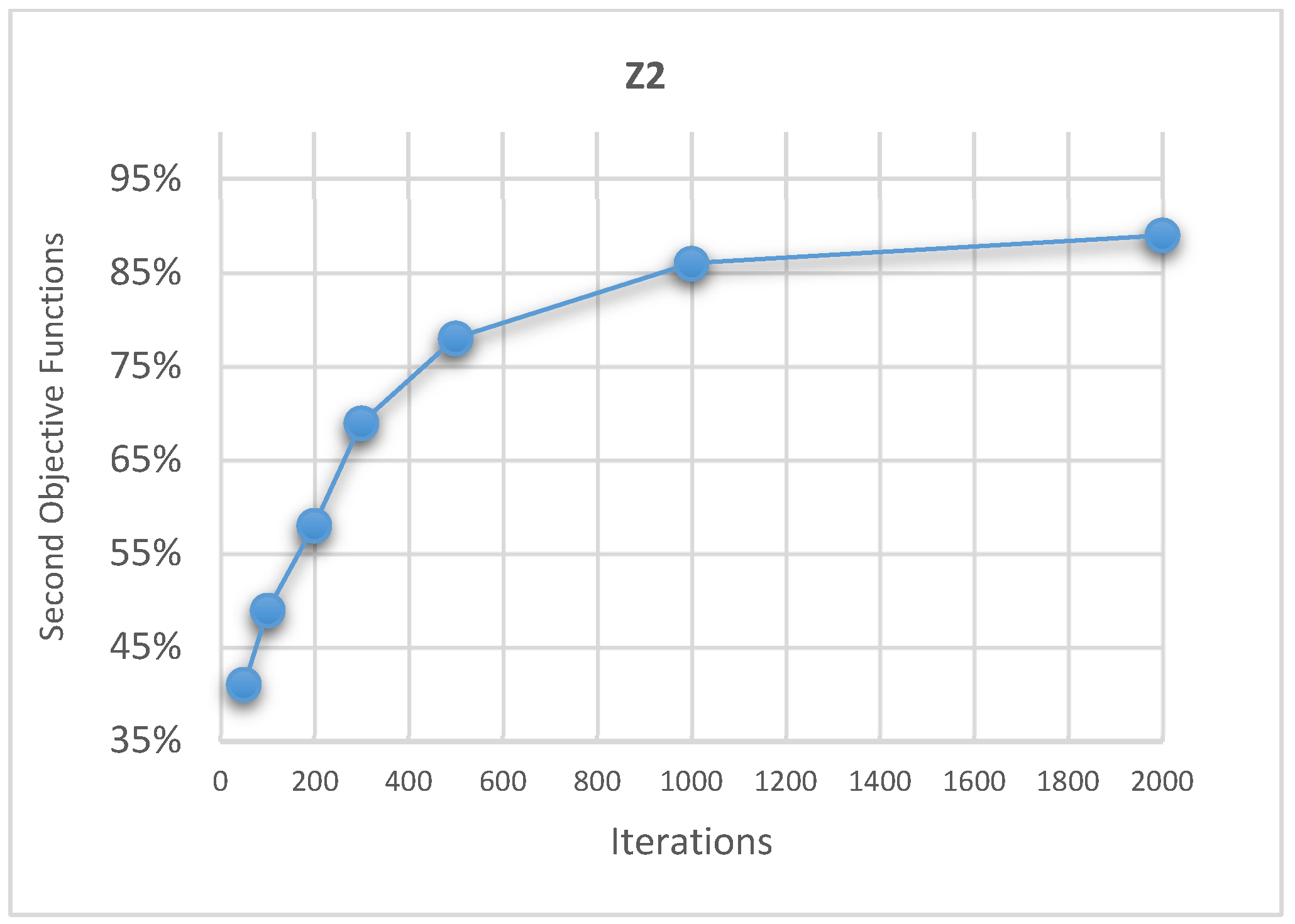
The second objective function displayed with Equation (4) aims to maximize the service coverage of generated transit routes in the network in terms of demand. Indeed, service coverage is referred to the percentage of the total estimated demand that may potentially be met by the public transit system.

3.2.4. Constraints

As discussed in Section 3.2, there are some assumptions that should be considered. The first is related to the length of the generated transit route. Equation (5) assures that the length of each route must be between a minimum and maximum length, which are determined based on factors such as driver fatigue and difficulty of maintaining the schedule. In other words, this equation prevents the generation of a route that is too long, because scheduling on a very long route can be difficult to be implement. Equation (6) shows that the distance between stop i and stop j should be between the minimum and maximum stop spacing distance. The maximum number of route constraints (transit route) in the network is shown by Equation (7).

$$L_{\min }^{r_m}\le L_{}^{r_m}\le L_{\max }^{r_m},\begin{array}{cc}& r_m\in R\end{array}$$

(5)

$$S_{\min }\le DI{S}_{ij}\le S_{\max },\begin{array}{cc}& i,j\in R\end{array}$$

(6)

$$N\le R_{\max },$$

(7)

Another important constraint, as shown in Equation (8), regards the bus headway feasibility in each generated transit route. This constraint provides the minimum and maximum headways. Equation (9) is designed to show the limitation of the available number of buses in the network. Indeed, this equation guarantees that the number of operating buses in an optimal public transit system cannot exceed the available number of buses. Equation (10) is the load factor constraint that assures that the maximum flow on each route cannot exceed the bus capacity on the same route.

$$B{H}_{\min }\le B{H}^{r_m}\le B{H}_{\max },\begin{array}{cc}& r_m\in R\end{array}$$

(8)

$${\displaystyle \sum _{r_m\in R}^{}F{S}^{r_m}=}{\displaystyle \sum _{r_m\in R}^{}\frac{R{T}^{r_m}}{B{H}^{r_m}}}\le B,\begin{array}{cc}& r_m\in R\end{array}$$

(9)

$$L{F}^{r_m}=\frac{Q_{\max }^{r_m}·B{H}^{r_m}}{S}\le L{F}_{\max },\begin{array}{cc}& r_m\in R\end{array}$$

(10)

Finally, Equation (11) displays the nature of variables that are used in our proposed model that would be integer numbers.

$$L^{r_m},DI{S}_{ij},D_{ij}^{r_m},T{R}_{ij}^{r_m},R{T}_{}^{r_m},B{H}_{}^{r_m},F{S}_{}^{r_m},L{F}_{}^{r_m},N\in Integer,\begin{array}{cc}& i,j,r_m\in R\end{array}$$

(11)

4. The Proposed Solution Methodology

The TNDP model is classified as an NP-Hard problem [18,19] and located as a non-convex (even concave) optimization problem [20]. Due to its hardness and difficulty to solve, researchers have tried to examine it from various viewpoints. As noted in the literature review, many developed heuristics, and meta-heuristic approaches are proposed by researchers to solving the TNDP model (see Table A1 in Appendix A). 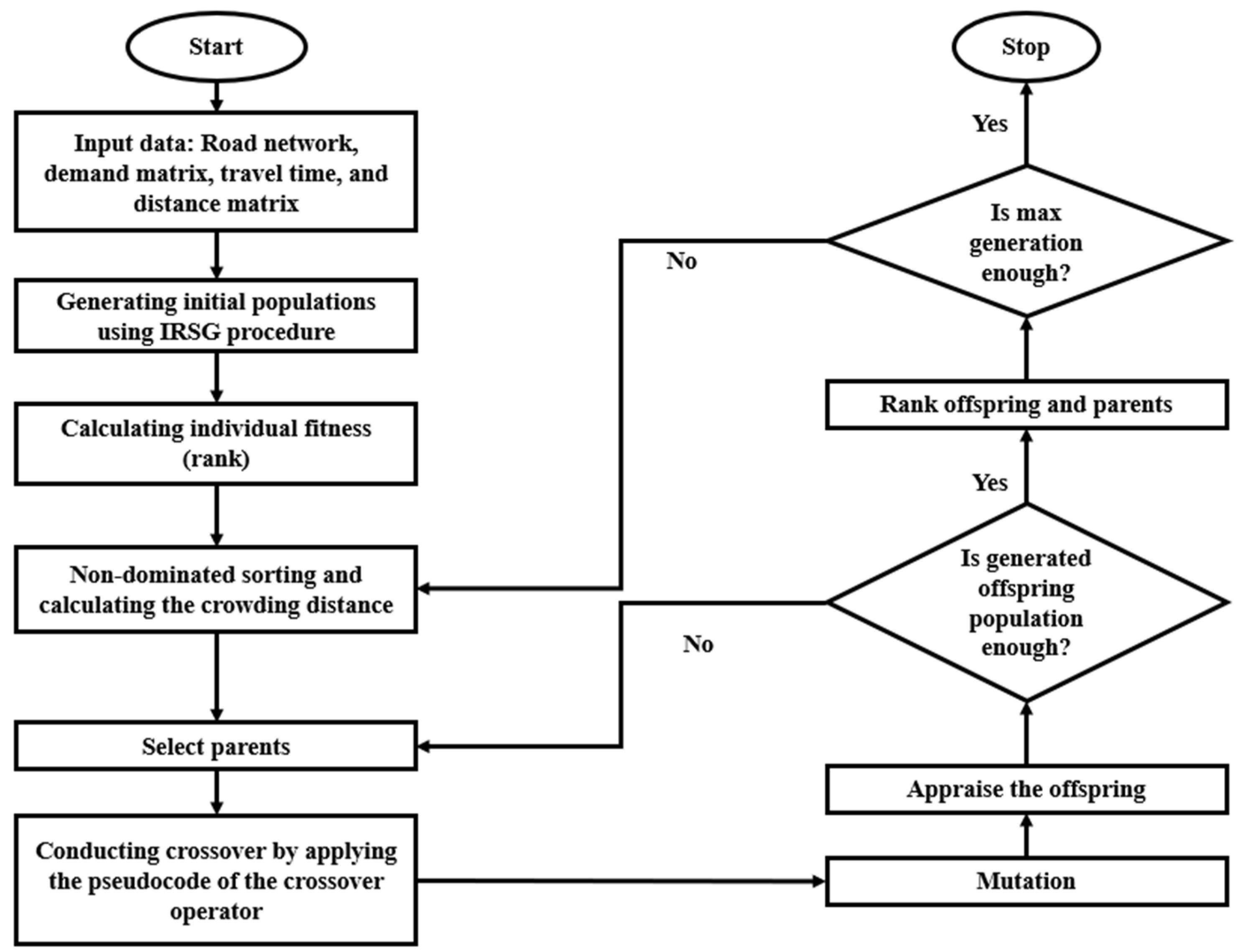Figure 2 shows the schematic view of the proposed IRSG procedure combined with NSGA-II algorithm in this study.

The extended version of the NSGA, called NSGA-II, is a fast and elitist multi-objective genetic algorithm introduced by Deb et al. [33]. This algorithm is an evolutionary multi-objective algorithm that improved upon NSGA. It is a population-based algorithm that would do unmistakable sorting to make the compromise between multi-objective functions. These characteristics enable NSGA II, rather than the best solution, to produce a set of non-dominated final solutions. The NSGA II algorithm is widely employed to solve multi-objective optimization problems in engineering and its applications. This algorithm is constructed based on the ranking selection method which is used to emphasize good points as well as the Niche Method to maintain stable sub-populations of generated good points [34].

4.1. Initial Route Set Generation (IRSG) Procedure

The Initial Route Set Generation (IRSG) procedure is combined with the NSGA-II algorithm to solve the proposed MOMINLP model. It should be noted that the proposed MOMINLP model in Section 3 is a non-linear model that needs to be solved by appropriate heuristic and meta-heuristic approaches [35,36,37]. Thus, the NSGA-II algorithm can be used to find promising, near-optimal solutions for the proposed MOMINLP model. Some studies have pointed out the robustness of the NSGA-II algorithm to pursue the distinguished benchmark problems without changing the value of algorithmic parameters [38,39].

In this study, each route is shown by an individual which is known as a transit route set from the given road network while each bus stop is shown by gen. Indeed, the IRSG algorithm presented here is based on a greedy algorithm that is a modification of Nikolić and Teodorović’s [36] initialization procedure.

Before presenting the proposed IRSG algorithm, a set of feasible transit routes needs to be produced in a way that does not require too much computational time and can lead to finding the best result. This would allow for the generation of a set of valid transit routes based on input data matrices, such as the distance matrix, the demand matrix, and the travel time matrix. The distance matrix is calculated and defined as the distance between each pair of the network. The demand matrix is the number of trips per time for each pair of nodes. The travel time matrix is calculated by the demand matrix toolbox of ArcGIS Pro 2.4.2 that shows the total travel time between each pair of nodes in the network. The proposed IRSG algorithm procedure starts with generating the initial route by an origin-destination matrix which is calculated by the demand matrix and the number of required transit routes. Next, bus stops are added into the initial route, considering constraints previously discussed. This is repeated until all required bus stops are added into the generated origin-destination terminal to complete the transit route generation. Algorithm 1 shows the pseudo-code of the proposed IRSG algorithm procedure in detail.

Algorithm 1. The pseudocode of IRSG algorithm.

1:  Input: Distance matrix (Distance), Origin-destination matrix (Origin-Destination), Minimum distance between two nodes (Min Distance Nodes), and Maximum distance between two nodes (Max Distance Nodes)

2:  Output: Valid chromosome (Initial Transit Routes)

3:  Initial Route = [Origin Destination Origin Destination]

4:  While true

5:   Bus Stop = Initial Route (size (Initial Route))

6:   Valid Distance = Find ((Distance (Bus Stop) > Min Distance Nodes) & (Distance (Bus Stop) < Max Distance Nodes))

7:    If size (Valid Distance) > 0 & all (is member (Valid Distance, Initial Route))

8:      Next Stop Status = True

9:      While Next Stop Status

10:        If size (Valid Distance) = 0

11:          break

12:        End

13:        Next Stop Index = Randi (1 size (Valid Distance))

14:        Next Stop = Valid Distance (Next Stop Index)

15:        If is empty (Find (Initial Route = Next Stop))

16:            Next Stop Status = False

17:            Initial Route = [Initial Route (end − 1) Next Stop Initial Route(end)]

18:        Else

19:            Valid Distance (Next Stop Index) = []

20:        End

21:      End

22:    Else

23:      Valid Chromosome = Initial Route

24:      break

25:    End

26:    If size (Initial Route) = Length Route

27:     Valid Chromosome = Initial Route

28:     Break

29:    End

30: End

4.2. Fitness Evaluation

After proposing the IRSG procedure for generating the transit route, the next step is to compute the fitness of each generated chromosome. In the NSGA-II algorithm, the fitness is calculated based on three factors including non-domination rank, crowding distance, and crowding comparison. These factors are calculated as follows:

1.

Fast non-dominated sort: the individual is the non-dominated solution if an individual objective function is not worse than the others. In the iterative process, every individual in non-inferior relationships is assigned to several fronts. Every individual is defined by a rank value of $P_{rank}^i$.

2.

Crowding distance: The average distance between two individuals must be measured to assess the distribution density of other individuals, which is known as the crowding distance. The distance is assigned for two boundary individuals to infinity and then distances are determined for other individuals through Equation (12).

$$c{d}^i={\displaystyle \sum _k^{}c{d}_k^i}={\displaystyle \sum _k^{}\frac{f_k^{i+1}-f_k^{i-1}}{f_{k,\max }^i-f_{k,\min }^i}}$$

(12)

where, $c{d}_k^i$ is the crowding distance of the kth objective function of the ith individual. $f_k^{i+1}$ and $f_k^{i-1}$ are the kth objective function values of the (i + 1) th and the (i − 1) th individuals, respectively. $f_{k,max}^i$ and $f_{k,min}^i$ are the maximum and minimum values of the kth objective function of the ith individual.

3.

Crowded comparison: if the ranks $P_{rank}^i$ and $P_{rank}^j$ are identical for two individuals i and j, the crowding distances of $c{d}_k^i$ and $c{d}_k^j$ should be compared. Then, if $P_{rank}^i<P_{rank}^j$ or $P_{rank}^i=P_{rank}^j$. but $c{d}_k^i>c{d}_k^j$, the ith individual is higher compared to the jth individual.

4.3. Tournament Selection

Before applying the genetic operation, the tournament selection should be performed. First, both parents are given the same chance to be selected. Second, parents S_i and S_k are chosen randomly and the parent who has the higher fitness value is selected. Finally, the second parent will be produced by repeating the process.

4.4. Modification Operators

The modification operators of the NSGA-II algorithm are employed to generate better solutions. The first operator is the crossover operator that ensures the exchange of genetic material between parents and creates chromosomes that are more likely better than the parents. Indeed, each gene is treated as a bus stop and by swapping genes of the chromosomes (transit route), the crossover of two-parent strings produces offspring as new solutions [40,41].

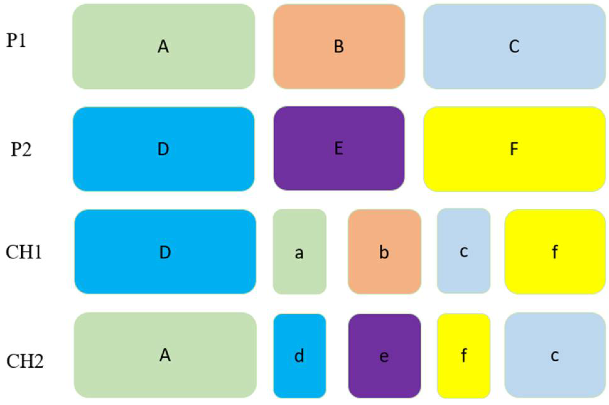
The crossover operator considered in this paper is schematically shown in Figure 3. Two parents P1 and P2 are chosen to be crossed to produce two children CH1 and CH2. The P1 and P2 are constituted by three parts of A, B, C and D, E, F. For building the first part of CH1, the first part of P2 (D) are copied. Then, for generating other parts of CH1 such as a, b, and c, these are obtained from the A, B, and C of P1. On the other hand, some elements that have already been added from P2 cannot be included again. This process is called nonrepetitive elements which avoid selecting the repeated elements into the CH1 and CH2. Finally, element f is selected from the set of F in P2. The same procedure is repeated to generate CH2. What is clear from Figure 3 is that the priority of generated new chromosomes by CH1 and CH2 are preserved by applying the proposed crossover operator. So, by doing this, the procedure generates feasible children’s solutions to the problem.

Algorithm 2 shows the pseudocode of the crossover operator which is proposed in this study, and it is written in MATLAB software 2021.

Algorithm 2. Pseudocode of Crossover operator.

1: If Crossover Type = 2,

2:   Feasibility_CH1 = 0

3:   Feasibility_CH2 = 0

4:   While Feasibility_CH1 + Feasibility_CH2 ~= 2

5:     C1, C2 = Creates two random numbers

6:     CH1 = [P1 (1: C1) P2 (C1 + 1: C2 − 1) P1 (C2: end)]

7:     CH2 = [P2 (1: C1) P1 (C1 + 1: C2 − 1) P2 (C2: end)]

8:    If CH1 is not Feasible

9:      Sub-tour elimination of CH1

10:    Feasibility_CH1 = 1

11:    End

12:  If CH2 is not Feasible

13:    Sub-tour elimination of CH2

14:    Feasibility_CH2 = 1

15:    End

16:    End

17:      End

After the crossover operator, the next operator is the mutation operator which starts playing a secondary role. To prevent a loss of potentially useful information, which can occasionally be caused by the crossover, the mutation operator is necessary to select one route among the generated routes to mutate the selected route. Every iteration can lead to solutions from the Pareto frontier and may only contain partial solutions to the original problem. New solutions generated following successive iterations may dominate the non-dominated solutions.

4.5. The NSGA-II Algorithm

In this study, the NSGA-II algorithm is employed to solve the proposed MOMINLP model. Indeed, the IRSG algorithm is proposed into the framework of NSGA-II to search for the approximate Pareto front in terms of the total travel time as well as service coverage area. These initial routes are considered into the framework of NSGA-II to generate higher quality final transit routes. Two objective functions are then calculated for each initial solution to calculate the fitness value. All initial solutions are regarded as parents and are used by genetic operators to produce offspring (i.e., tournament selection, crossover, and mutation operators). Algorithm 3 shows the NSGA-II algorithm to solve the proposed MOMINLP model in Section 3.

Algorithm 3. The NSGA-II algorithm.

1: Input: Road network, demand matrix, travel time, distance matrix

2: Output: Passenger time, operating costs, and number of required buses on each route.

3: Determining transit route of the network by IRSG procedure to generate the initial solution

4: Setting the parameters as the author has brought in Table 1. Parameters of running the algorithm. Name of Parameters. Quantity Descriptions nPop 50 Number of chromosomes or individual (transit route) MaxIteration 500 Maximum number of iterations nVar 667 Number of gens (Bus Stops) PMutation 0.4 Probability of mutation PCrossover 0.8 Probability of crossover VarMin 25 bus stops Minimum number of stations in each generated route VarMax 68 bus stops Maximum number of stations in each generated route nRoutes 16, 18, 20, 22, 24 transit routes Total number of required routes determined by transit planner AVG_Speed 30 mph The average speed of bus during the operation Headway_Min 15 min/bus The minimum headway in any route Headway_Max 30 min/bus The maximum headway in any route Max_Buses 39 The total number of available buses and then assign to each route

5: Calculating the frequency of each route

6: Evaluating the fitness based on three factors discussed in Section 4.2.

7: Set gen = 0,

8: While gen < Max gen

9:    Select parents using tournament selection

10:  Generate offspring by applying crossover and mutation

11:  Update frequency on each route

12:  Evaluate the fitness

13:  Accumulate the population of offspring and parents

14:  Assign rank to population

15:  Computing the crowding distance

16:  Gen = Gen + 1

17: End while

18: Final population (transit routes)

After applying the NSGA-II algorithm, the fleet size (operator costs) for each generated route by IRSG procedure is calculated along with the frequency of each route. Then, the total travel time of passengers (user costs), the length of each generated route, the average load factor of all transit routes, and the total amount of demand satisfied on each route (demand coverage) are computed for the network of FMA.

5. Case Study

The Fargo-Moorhead metropolitan area is constituted primarily of the city of Fargo in the state of North Dakota and the city of Moorhead in the state of Minnesota. Fargo has a land area of 128.82 square kilometers and a population of 123,736, while Moorhead has a population of 42,939 and a land area of 57.67 square kilometers [42]. These two cities are located on the North Dakota–Minnesota state border and are separated by the Red River. The city of Fargo has the highest population in the state of North Dakota [42].

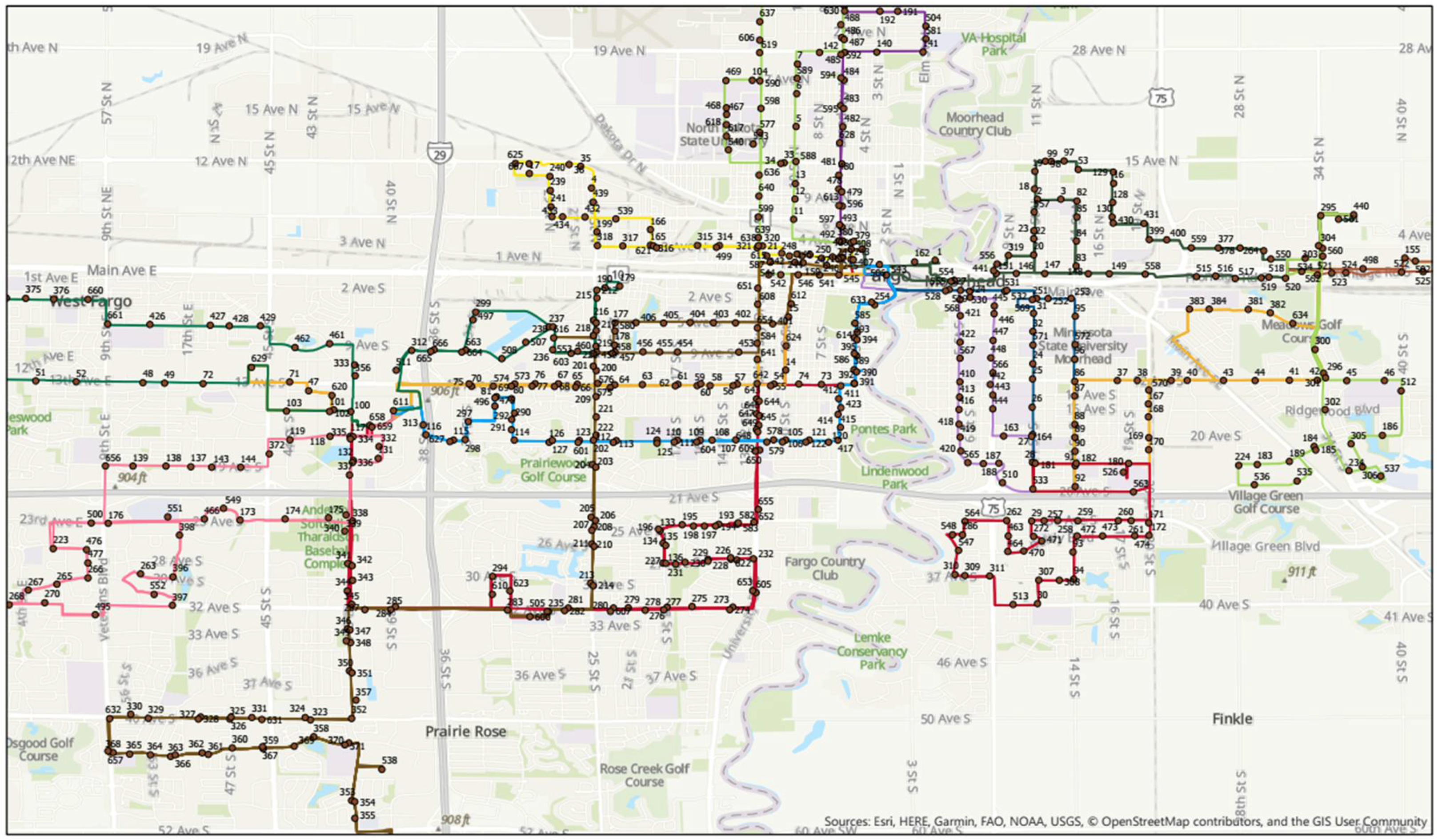
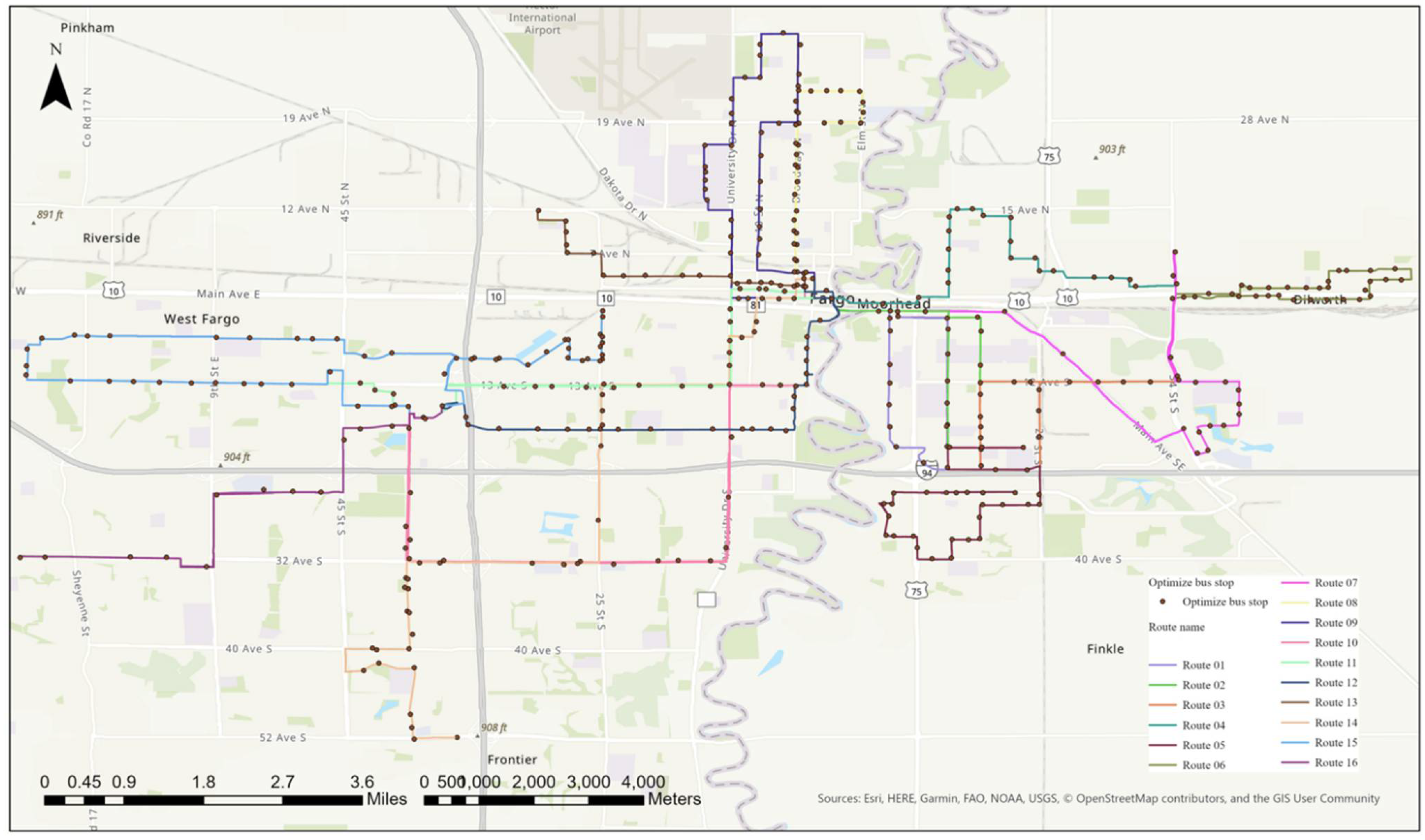
MATBUS is the public transportation provider in FMA. This transit system has 16 routes which are numbered from 1 through 16. The network is constructed by 667 nodes, 974 links, and 193,449 total transit demand and is shown in Figure 4. Public transportation in FMA can be seen by the MATBUS application [43]. In the MATBUS application, all the routes are shown by numbers, and by clicking on each route, transit users can see when the first available bus will arrive, how many buses there are in a specific route, the locations of bus stops, and the locations of buses and the direction in which they are moving. More interestingly, this application shows all the available buses in the total network. The background of this application is designed on Google Maps software.

As previously mentioned, the main purpose of this study is to design an efficient public transit system in the FMA to improve upon the existing network for transporting passengers from origins to destinations by applying an efficient NSGA-II algorithm. The benefit of using the NSGA-II algorithm is to find the best route among the existing routes near the optimal solution. The proposed algorithm in this study is coded on MATLAB software 2021 and it consisted of 16 modules such as Transportation Cost, Sort of Population, Roulette wheel selection, remove a repetitive element, Read GIS Data, Pre-processing, Plots Costs, Non-Dominated Sorting, Mutation, Dominates, Crossover, Create Valid Chromosome, Create GIS Information, Count Bus Passenger and Calculating Crowding Distance. The MATLAB software 2021 is connected to a worksheet in MS-Excel to get the information as needed, such as GIS Data, travel demand, and travel time of passengers. 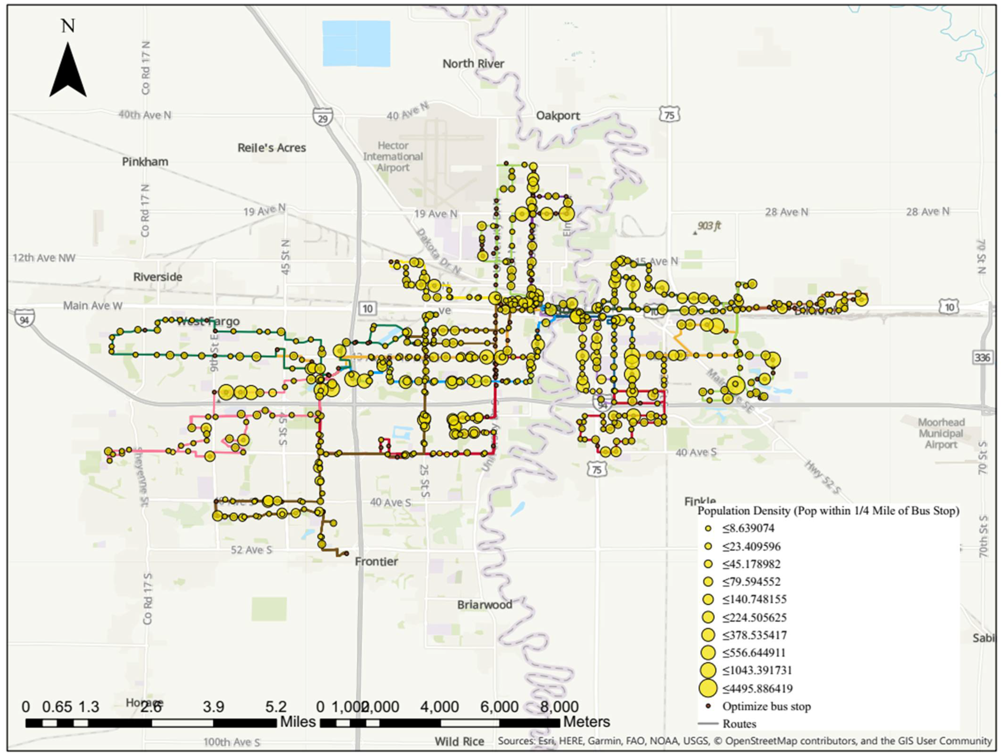Figure 4 shows the existing routes of the FMA network on ArcGIS Pro version 2.4.2, where each route is shown with different colors and each bus stop is identified by an index number to allow us for easy tracking. Moreover, Figure 5 displays the population density near each current bus stop by 10 different ranges. What is clear from Figure 5 is that in some regions of Fargo, the number of people who are living near the bus stop is more than in other areas of the city.

Three matrices are used as the main input data. These include travel time, total distance, and demand metrics. The demand matrix is constructed by a size of 218,089 elements, including 76,121 pairs of nodes with non-zero demand and 117,328 pairs with zero demand. The travel time and distance matrices have the same size as the demand matrix.

6. Results and Discussions

The proposed NSGA-II algorithm has been conducted on the FMA network to compare the effectiveness of the NSGA-II algorithm with the performance of the existing public transit system. Some researchers tested their proposed solution approach on the popular networks such as Mandl’s Swiss, Mumford1, Mumford2 and Mumford3, and Sioux Falls network to investigate its effectiveness by solving their models [1,13,24,36,44,45].

6.1. Defining Parameters Value

The proposed NSGA-II algorithm is coded on MATLAB software 2021 on a computer with a 1.60 GHz Intel Core TM i7-4200 CPU with 16GB of RAM. The performance of the proposed NSGA-II algorithm depends on the parameters defined in Table 1, which include the number of populations, number of generations, number of existing bus stops, probability of crossover and mutation, minimum and maximum length of each transit route, number or routes the planner decides to generate, the average speed of existing buses operating, minimum and maximum bus headway, and maximum number of available buses in the network.

In this study, five scenarios are considered, each with a different number of transit routes, as shown in

Table 2. Definition of scenarios based on number of routes defined.

Scenario	Number of Defined Routes
1	16
2	18
3	20
4	22
5	24

, to easily compare the newly designed network with the existing network. As previously discussed in Section 5, the existing network of FMA is based on 16 transit routes. Therefore, to compare the newly designed network with the existing network, scenario 1 should be considered.

6.2. Result of the Proposed IRSG Algorithm

The proposed IRSG algorithm generates many high-quality initial solutions that are inputted into the NSGA-II algorithm. In Figure 6, we have shown one set of near-optimal initial solutions. Because five different scenarios were considered, many routes were generated (a total of 100 transit routes). For the sake of brevity, only scenario 1 (16 routes) is reported in Figure 6.

Table 3. Set of origin and destination bus stops for different scenarios.

Route Size	16		18		20		22		24
Route Number	Origin	Destination	Origin	Destination	Origin	Destination	Origin	Destination	Origin	Destination
1	258	257	110	111	357	44	445	256	130	129
2	143	142	212	166	318	317	160	137	38	37
3	165	8	73	72	80	405	357	44	445	256
4	42	41	258	257	110	111	318	317	160	137
5	410	104	143	142	212	166	80	405	357	44
6	131	322	165	8	73	72	110	111	318	317
7	128	127	42	41	258	257	212	166	80	405
8	467	439	410	104	143	142	73	72	110	111
9	239	235	131	322	165	8	258	257	212	166
10	410	349	128	127	42	41	143	142	73	72
11	281	279	467	439	410	104	165	8	258	257
12	98	16	239	235	131	322	42	41	143	142
13	330	130	410	349	128	127	410	104	165	8
14	283	281	281	279	467	439	131	322	42	41
15	237	236	98	16	239	235	128	127	410	104
16	73	72	330	130	410	349	467	439	131	322
17	-	-	283	281	281	279	239	235	128	127
18	-	-	237	236	98	16	410	349	467	439
19	-	-	-	-	330	130	281	279	239	235
20	-	-	-	-	283	281	98	16	410	349
21	-	-	-	-	-	-	330	130	281	279
22	-	-	-	-	-	-	283	281	98	16
23	-	-	-	-	-	-	-	-	330	130
24	-	-	-	-	-	-	-	-	283	281

summarizes the origins and destinations for each route for all five scenarios. The reason for considering the various scenarios is that if planners require a different number of transit routes, the origin-destination terminal matrix calculated by the proposed NSGA-II algorithm changes. Considering different scenarios can help the planner decide how many transit routes are required to control the operating and user costs of the network. Therefore, Table 3 summarizes and reports the various scenarios of transit routes that are acquired by the IRSG algorithm designed in Section 4.1. As shown in Table 3, when the number of predefined transit routes changes by the planner, the origin and destination bus stop also change.

6.3. Result of the Proposed NSGA-II Algorithm

This section presents the result of the proposed MOMINLP model in Section 3 by applying the NSGA-II algorithm solution methodology.

Table 4. Comparing the number of bus stops in each route between existing and optimized FMA network.

Route Number	Existing FMA Network (Number of Bus Stops)	Optimized FMA Network (Number of Bus Stops)	Percentage of Change (%)
1	31	21	−48%
2	29	23	−26%
3	34	29	−17%
4	56	41	−37%
5	36	38	+5%
6	31	36	+14%
7	27	31	+13%
8	34	39	+13%
9	57	51	−12%
10	88	67	−31%
11	51	45	−13%
12	56	46	−22%
13	38	33	−15%
14	98	71	−38%
15	62	49	−27%
16	46	47	+2%

compares the route length of the optimized designed network with the existing network of FMA. As previously mentioned, the FMA network is constituted by 16 routes and constructed by 667 nodes, 974 links, and 193,449 total transit demands, including 76,121 pairs of nodes with non-zero demand and 117,328 pairs with zero demand. Therefore, the existing network is compared with scenario 1 (16 routes). As shown in Table 4, the number of bus stops in each transit route has changed. For instance, route numbers 1, 4, and 14 with 31, 56, and 98 bus stops are dramatically decreased to 21, 41, and 71 bus stops in an optimized designed network. This tells us that the proposed NSGA-II algorithm methodology could considerably decrease the total number of bus stops in the network by meeting two objective functions of demand coverage maximization and minimization of passenger travel time.

Moreover, Figure 7 compares the length of the optimized designed network (scenario 1) with the existing network of FMA. What is clear from Figure 7 is that in an optimized designed network, the length of each route is decreased. Another thing that is clear from Figure 7 is that the highest decrease happened for route numbers 4, 10, and 14 with 5130, 7326, and 9192 m, respectively.

After generating the initial route of the transit network and assigning the required number of buses to each generated route, the existing number of buses operating in the FMA network are compared with the optimal number of buses that could result from the proposed NSGA-II algorithm. Figure 8 displays the number of buses between the optimized network and the existing network for scenario 1 (16 routes). In this study, it is assumed that the minimum and maximum bus headways are 15 and 30 min. Therefore, the frequency of each route varies between 2 and 4 buses per hour. By running the proposed NSGA-II algorithm, the total number of buses decreases from 39 (existing network of FMA) to 35 buses (optimized designed network). Indeed, the proposed algorithm could save 4 buses, thereby reducing operating costs.

More interestingly, the optimal bus headway was computed for each generated route of the optimized network to compare them with the existing bus headway of the FMA network. As can be seen from

Table 5. Comparing the number of bus headway of different routes between existing and optimized network.

Route Number	Existing FMA Network (Bus Headway)	Optimized FMA Network (Bus Headway)
1	30	30
2	30	30
3	30	30
4	30	30
5	30	30
6	30	30
7	30	30
8	30	30
9	30	30
10	20	30
11	12	15
12	30	30
13	20	30
14	30	30
15	15	20
16	30	30

, only the bus headway of route numbers 10, 11, 13, and 15 have been changed (bold numbers).

6.4. Sensitivity Analysis

This sub-section is devoted to sensitivity analysis on some input parameters that have a direct impact on the solutions provided by the NSGA-II algorithm. These parameters include the probability of crossover, number of iterations (generations), number of candidate routes (five scenarios defined in Table 2), and maximum number of buses.

The effects of changing the value of penalty coefficients W₁ and W₂ on the first objective function for scenarios 1 to 5 are shown in Figure 9. Two changes in the value of penalty coefficients are considered. When the number of routes increases from scenario 1 (16 transit routes) to scenario 5 (24 transit routes), the value of Z₁ (first objective function) increases considerably when W₁ = 0.2 and W₂ = 0.8. This is because more weight is assigned to the second part of the first objective function as well as it is more costly to provide more routes. The same trend has happened for the condition that W₁ = 0.5 and W₂ = 0.5, but with a flatter slope. More interestingly, increasing the number of routes from scenario 1 to scenario 5 also increases the value of the second objective function, as shown in Figure 10. Indeed, by changing the routes, the slightly increasing trends are achieved by the second objective function. The second objective function maximizes the service coverage of the network. Figure 10 shows that scenario 5 (24 transit routes) covers the highest percentage of demand on the network, at 93 percent.

Figure 11 explains the convergence process of running the NSGA-II algorithm from 50 to 2000 generations by considering two penalty coefficients of W₁ = 0.2, W₂ = 0.8, and W₁ = 0.5, W₂ = 0.5 (scenario 1) for the first objective function. Figure 11 shows that the algorithm needs to run around 2000 iterations, because of the complexity of the proposed MOMINLP model. Additionally, at the start of the generation, the value of the first objective function starts decreasing suddenly, and then it tends to be stable gradually at the end of the generation. This trend shows the convergence process of running the NSGA-II algorithm. The optimum iteration that can satisfy the reasonable result is about 500 generations for the two conditions defined for the first objective function. The reverse trend happened for the second objective function, which is shown in Figure 12. Indeed, when the number of generations for the second objective function is increased from 50 to 2000, the graph at the beginning started to abruptly grow and then reached the stable line with the generation of 2000.

The impacts of changing values for crossover probability were also examined. Figure 13 displays the impacts of different crossover probabilities on the two objective functions when W₁ = 0.2, W₂ = 0.8, for scenario 1. When the probability of crossover increases, the value of the first and second objective functions are shown to also change. This figure shows that as much as the probability of crossover increases, a better solution can be reached for both objective functions. Therefore, the planner can do a trade-off between the two objective functions to select the best operator value for running the model to get the solution by satisfying two opposite objective functions values.

Finally, the effects of the number of available buses in the network were analyzed for scenario 1. As shown in Figure 14, when the number of buses increases, the total value of the first objective function that is constituted by user costs and operator costs also increases. The slope of the line in Figure 14 increases when the number of buses is greater than 39, showing that costs are increasing at an increasing rate. This is due to the penalty assigned to the second part of the first objective function when the maximum number of available buses exceeds 39 buses. In this way, the planner can decide based on their budget how many buses to assign.

The Pareto optimal solutions for the first and second objective functions in scenario 1 (16 transit routes) with two different conditions of (W1 = 0.2, W2 = 0.8) and (W1 = 0.5, W2 = 0.5) is reported in Figure 15. The first thing that is visible from Figure 15 is that when the value of the first objective function increases, the value of the second objective function decreases, which highlights the conflicting nature of the two objective functions. The solutions shown in Figure 15 in the Pareto front are non-dominated solutions. It means that no solution in the frontier is better than another. Another important thing that Figure 15 says is that the obtained Pareto optimal set has a varied set of solutions that allow the planner to choose a desirable set of passenger interest or operator interest or a combination of two of them among the non-dominated frontier without linear trade-off.

Table 6. Comparing the result of the optimized network with the existing network (scenario 1).

Studied Variables	Existing FMA Network	Optimized FMA Network	Difference (Percent)
Total user costs (minutes)	1,218,648	1,103,704	−9.4
Total operating costs (minutes)	112,200	90,720	−19.14
Total number of operating buses (buses)	39	35	−10.25
The average frequency of all routes (buses per hours)	2.43	2.18	−10.28
Average length of all routes (km)	14.560	11.922	−18.11
Average load factor of all routes (per buses)	68.25%	72.73%	+6.5

summarizes one of the Pareto frontiers of the optimal solution achieved by running the NSGA-II algorithm to verify the effectiveness of the proposed solution methodology. The table shows six variables to compare the result obtained by running the algorithm with the existing network. The number of operating buses in the existing network decreased from 39 to 35 in the optimized network. This outcome was obtained by generating a new set of transit routes by proposing the IRSG procedure. On the other hand, changing the sequence of bus stops could affect the result of the existing network. Another performance metric used to compare the existing network with the optimized network was to consider the load factor of each route to prevent the maximum flow on any route from exceeding the capacity on that route. The load factor is shown to increase in the optimized network. Another performance metric was the average frequency of all routes, which decreased from 2.43 to 2.18 buses per hour.

7. Conclusions

This paper studied the TNDP model in public transit systems. The TNDP model aims to determine the set of routes and frequency on each route for public transportation systems. The TNDP model is classified as an NP-Hard combinatorial optimization problem [18,19], whose optimal solution is difficult to be found. In this study, by proposing the IRSG algorithm procedure, the TNDP model is solved to generate a set of transit routes. Indeed, the purpose of the proposed IRSG algorithm was to produce high-quality initial route set solutions to reach better optimization procedures. Second, the MOMINLP model is proposed to formulate the frequency setting problem on each route by minimizing the total travel time of passengers (user costs) to serve a greater number of travelers and minimizing operator costs simultaneously as well as maximizing the service coverage area near all the existing bus stops in FMA network.

Because of the complexity of the proposed model, the NSGA-II algorithm was applied, considering two objective functions at the same time. Based on the nature of the two proposed objective functions, the NSGA-II algorithm is employed to produce a Pareto front optimal solution. The obtained solutions by the proposed algorithm in the Pareto front are non-dominated solutions which means that no solutions in the frontier are better than others. On the other hand, the obtained solutions by Pareto frontier are the set of solutions that encourage the planner to choose a solution to satisfy passenger or operator interest as much as they want.

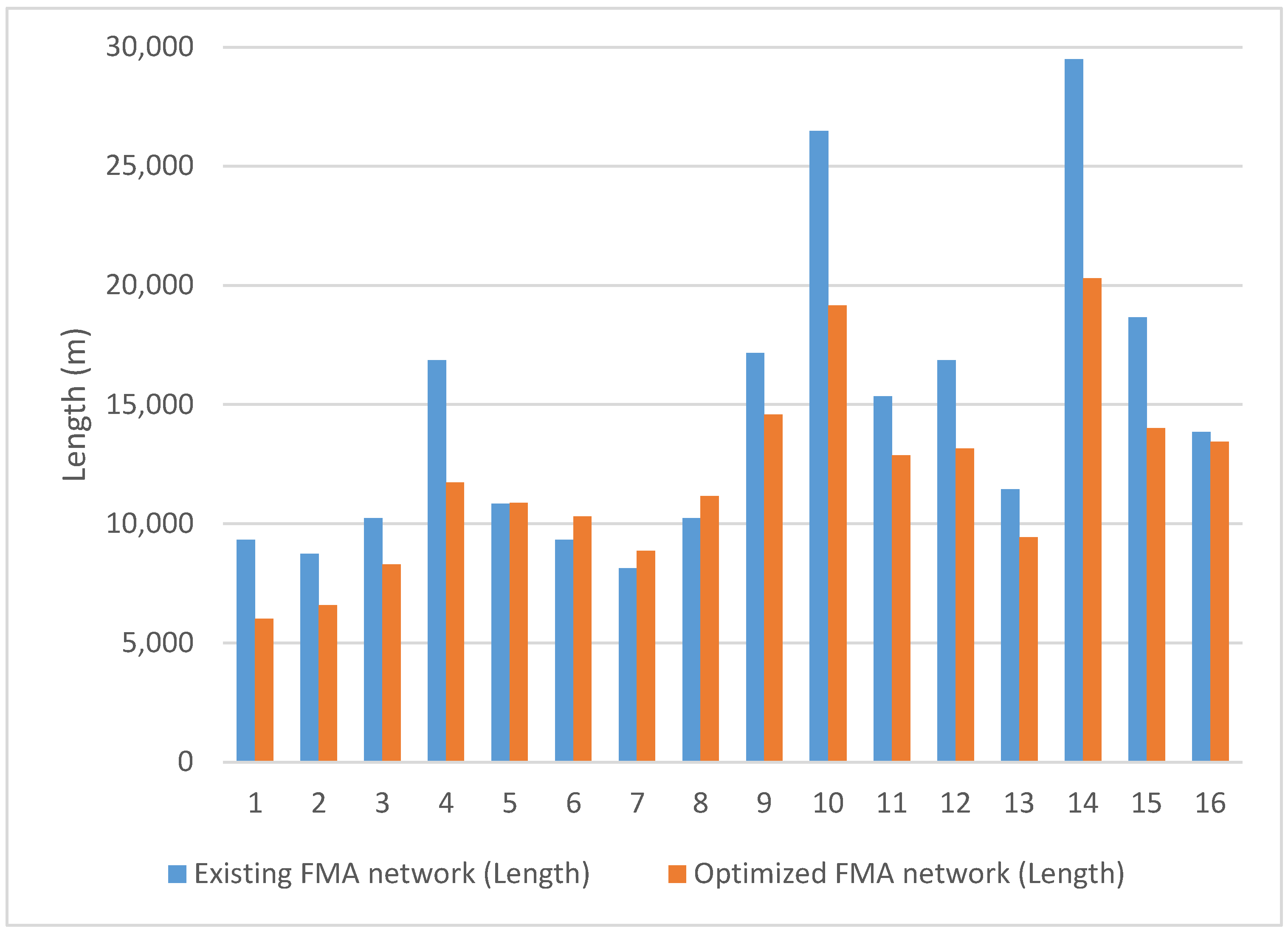
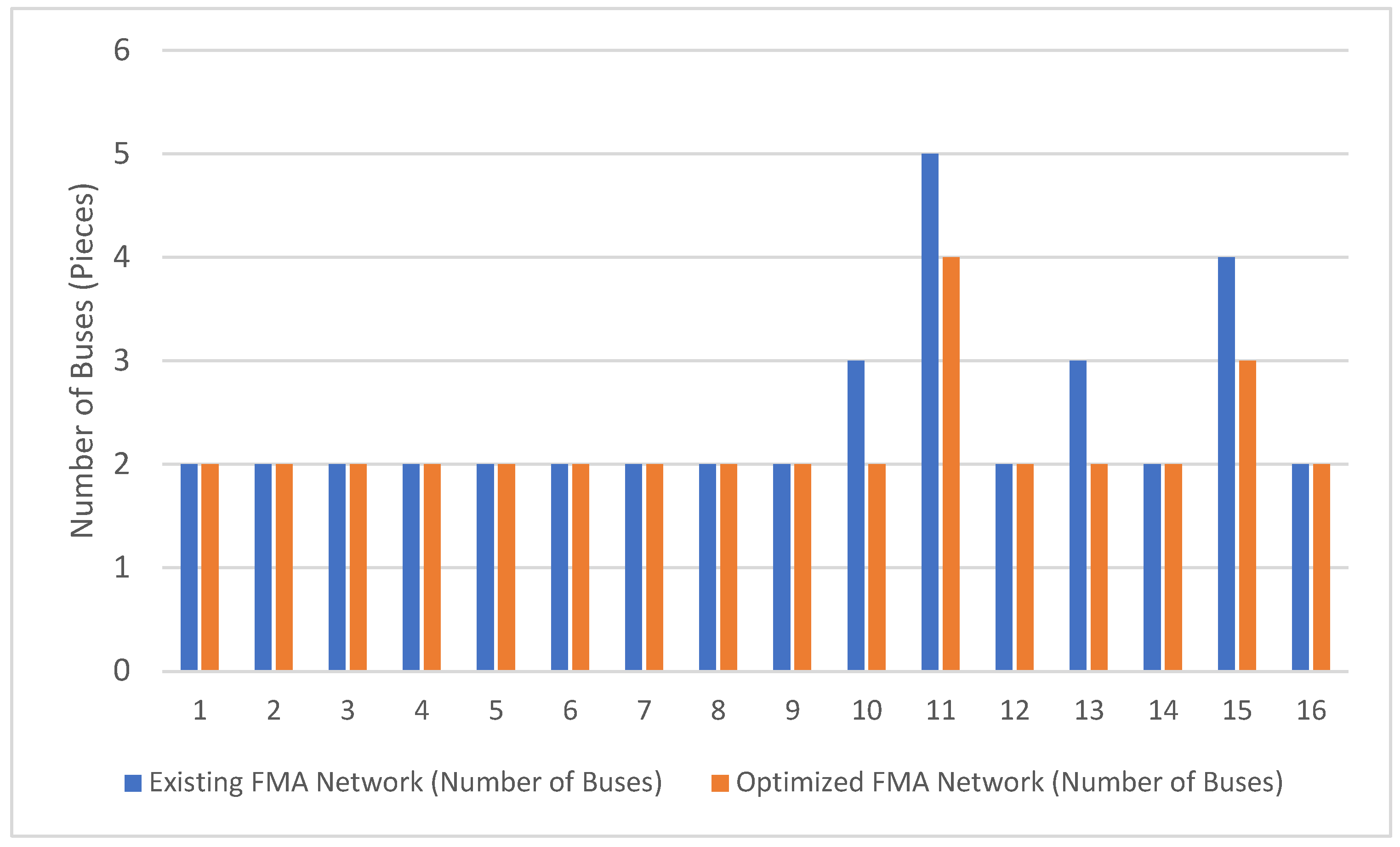
This paper for the first time considered the case study of FMA to improve the existing condition of operating buses and transit routes. Indeed, by applying the model to the case study, the existing network could be improved in several ways. The optimized network is shown to meet more demand, reduce travel time of passengers, and require fewer operating buses. Total user costs could decrease more than 9 percent and operating costs by 19 percent. Average route length in the new network decreased from 14,560 m to 11,922 m, showing that the proposed IRSG algorithm could produce a set of efficient transit routes. The load factors could increase from 68 to 73 percent. Finally, the number of buses operating in the network decreased by 4 buses. Results show that the proposed methodology works remarkably well.

By conducting this research, people living in FMA can benefit in terms of improved public welfare and access to social needs. By reducing the number of operating buses, the amount of pollution into the air can be decreased. Moreover, designing a new set of transit routes could considerably decrease the investment in public transit systems in FMA. Alternatively, the cost savings provided by the model could allow the transit agency to expand its service, either by providing more routes or improving frequency so that it can better serve the transportation needs of the public. Moreover, by reducing the total travel time of passengers, people are more likely to use the bus instead of using their vehicles, which leads to a decrease in fuel consumption. Furthermore, by maximizing the service coverage, the optimized network could meet more of the demand. Therefore, by improving the existing network of FMA in North America, more passengers can be served. While this model was shown to be successfully applied to the FMA network, it could be applied to transit networks in other cities. Results show that transit systems in small urban areas, which are challenged to provide efficient service in an environment of dispersed demand and low population densities, can improve their system design using this optimization model.

For future research, the proposed algorithm can be tested on the popular Mandl’s Swiss Network, which is proposed by Mandl [21]. Moreover, the model can be expanded by considering congestion, vehicle performance, different policy requirements, new bus stop locations, and making some simple modifications to the proposed objective function by including cost minimization and maximization of the number of trips without transfers. The dynamic design of bus services on each generated route can be considered as a real-time condition in future work. Finally, other heuristics algorithms such as multi-objective particle swarm optimization with multiple search strategies, bee colony, and tabu-search can be an alternative for this study to generate better results.

References

1. Chakroborty, P.; Wivedi, T. Optimal Route Network Design for Transit Systems Using Genetic Algorithms. Eng. Optim. 2002, 34, 83–100. [Google Scholar] [CrossRef]
2. Yang, Z.; Yu, B.; Cheng, C. A Parallel Ant Colony Algorithm for Bus Network Optimization. Comput. Civ. Infrastruct. Eng. 2006, 22, 44–55. [Google Scholar] [CrossRef]
3. Chen, L.-W.; Hu, T.-Y.; Shih, L.-C.; Liao, T.-Y. An ε-Constraint Multi-objective Algorithm for Transit Route Design with Subsidy Consideration. In Proceedings of the 2018 IEEE International Conference on Service Operations and Logistics, and Informatics (SOLI), Singapore, 31 July–2 August 2018; pp. 163–168. [Google Scholar]
4. Zhao, F.; Zeng, X. Simulated Annealing–Genetic Algorithm for Transit Network Optimization. J. Comput. Civ. Eng. 2006, 20, 57–68. [Google Scholar] [CrossRef]
5. Yu, B.; Yang, Z.-Z.; Jin, P.-H.; Wu, S.-H.; Yao, B.-Z. Transit route network design-maximizing direct and transfer demand density. Transp. Res. Part C Emerg. Technol. 2012, 22, 58–75. [Google Scholar] [CrossRef]
6. Kim, M.; Kho, S.-Y.; Kim, D.-K. A Transit Route Network Design Problem Considering Equity. Sustainability 2019, 11, 3527. [Google Scholar] [CrossRef] [Green Version]
7. Ceder, A. Public Transit Planning and Operation: Theory, Modeling and Practice; Elsevier: Oxford, UK, 2007. [Google Scholar]
8. Ibarra-Rojas, O.; Delgado, F.; Giesen, R.; Muñoz, J. Planning, operation, and control of bus transport systems: A literature review. Transp. Res. Part B Methodol. 2015, 77, 38–75. [Google Scholar] [CrossRef]
9. Ceder, A.; Wilson, N.H. Bus network design. Transp. Res. Part B Methodol. 1986, 20, 331–344. [Google Scholar] [CrossRef]
10. Bussieck, M.R.; Kreuzer, P.; Zimmermann, U.T. Optimal lines for railway systems. Eur. J. Oper. Res. 1997, 96, 54–63. [Google Scholar] [CrossRef]
11. Binder, S.; Maknoon, Y.; Bierlaire, M. The multi-objective railway timetable rescheduling problem. Transp. Res. Part C Emerg. Technol. 2017, 78, 78–94. [Google Scholar] [CrossRef] [Green Version]
12. Gallo, M.; Montella, B.; D’Acierno, L. The transit network design problem with elastic demand and internalisation of external costs: An application to rail frequency optimisation. Transp. Res. Part C Emerg. Technol. 2011, 19, 1276–1305. [Google Scholar] [CrossRef]
13. Fan, W.; Machemehl, R.B. Tabu Search Strategies for the Public Transportation Network Optimizations with Variable Transit Demand. Comput. Civ. Infrastruct. Eng. 2008, 23, 502–520. [Google Scholar] [CrossRef]
14. Cipriani, E.; Gori, S.; Petrelli, M. Transit network design: A procedure and an application to a large urban area. Transp. Res. Part C Emerg. Technol. 2012, 20, 3–14. [Google Scholar] [CrossRef]
15. Yan, Y.; Liu, Z.; Meng, Q.; Jiang, Y. Robust Optimization Model of Bus Transit Network Design with Stochastic Travel Time. J. Transp. Eng. 2013, 139, 625–634. [Google Scholar] [CrossRef]
16. Islam, K.A.; Moosa, I.M.; Mobin, J.; Nayeem, M.A.; Rahman, M.S. A heuristic aided Stochastic Beam Search algorithm for solving the transit network design problem. Swarm Evol. Comput. 2019, 46, 154–170. [Google Scholar] [CrossRef]
17. Yu, B.; Yang, Z. Optimizing bus transit network with parallelant colony algorithm. In Proceedings of the Eastern Asia Society for Transportation Studies, Tokyo, Japan; 2005; Volume 5, pp. 374–389. [Google Scholar]
18. Israeli, Y.; Ceder, A. Transit Route Design Using Scheduling and Multiobjective Programming Techniques. In Multiple Criteria Decision Making; Springer: Berlin/Heidelberg, Germany, 1995; Volume 430, pp. 56–75. [Google Scholar]
19. Magnanti, T.L.; Wong, R.T. Network Design and Transportation Planning: Models and Algorithms. Transp. Sci. 1984, 18, 1–55. [Google Scholar] [CrossRef] [Green Version]
20. Newell, G.F. Some Issues Relating to the Optimal Design of Bus Routes. Transp. Sci. 1979, 13, 20–35. [Google Scholar] [CrossRef]
21. Mandl, C.E. Evaluation and optimization of urban public transportation networks. Eur. J. Oper. Res. 1980, 5, 396–404. [Google Scholar] [CrossRef]
22. Dubois, D.; Bel, G.; Llibre, M. A Set of Methods in Transportation Network Synthesis and Analysis. J. Oper. Res. Soc. 1979, 30, 797–808. [Google Scholar] [CrossRef]
23. Krivda, V.; Petru, J.; Macha, D.; Novak, J. Use of Microsimulation Traffic Models as Means for Ensuring Public Transport Sustainability and Accessibility. Sustainability 2021, 13, 2709. [Google Scholar] [CrossRef]
24. Baaj, M.H.; Mahmassani, H.S. An AI-based approach for transit route system planning and design. J. Adv. Transp. 1991, 25, 187–209. [Google Scholar] [CrossRef]
25. Lampkin, W.; Saalmans, P.D. The Design of Routes, Service Frequencies, and Schedules for a Municipal Bus Undertaking: A Case Study. J. Oper. Res. Soc. 1967, 18, 375. [Google Scholar] [CrossRef]
26. Chakroborty, P. Genetic Algorithms for Optimal Urban Transit Network Design. Comput. Civ. Infrastruct. Eng. 2003, 18, 184–200. [Google Scholar] [CrossRef]
27. Szeto, W.; Wu, Y. A simultaneous bus route design and frequency setting problem for Tin Shui Wai, Hong Kong. Eur. J. Oper. Res. 2011, 209, 141–155. [Google Scholar] [CrossRef] [Green Version]
28. Carrese, S.; Gori, S. An Urban Bus Network Design Procedure. In Applied Optimization; Kluwer Academic Publishers: Boston, MA, USA, 2004; pp. 177–195. [Google Scholar]
29. Zhao, H.; Xu, A.; Jiang, R. The Memetic algorithm for the optimization of urban transit network. Expert Syst. Appl. 2015, 42, 3760–3773. [Google Scholar] [CrossRef]
30. Buba, A.T.; Lee, L.S. Hybrid Differential Evolution-Particle Swarm Optimization Algorithm for Multiobjective Urban Transit Network Design Problem with Homogeneous Buses. Math. Probl. Eng. 2019, 2019, 5963240. [Google Scholar] [CrossRef] [Green Version]
31. Nnene, O.A.; Joubert, J.W.; Zuidgeest, M.H. Transit network design with meta-heuristic algorithms and agent based simulation. IFAC-PapersOnLine 2019, 52, 13–18. [Google Scholar] [CrossRef]
32. Chen, J.; Liu, Z.; Wang, S.; Chen, X. Continuum approximation modeling of transit network design considering local route service and short-turn strategy. Transp. Res. Part E Logist. Transp. Rev. 2018, 119, 165–188. [Google Scholar] [CrossRef]
33. Deb, K.; Pratap, A.; Agarwal, S.; Meyarivan, T. A fast and elitist multiobjective genetic algorithm: NSGA-II. IEEE Trans. Evol. Comput. 2002, 6, 182–197. [Google Scholar] [CrossRef] [Green Version]
34. Srinivas, N.; Deb, K. Muiltiobjective Optimization Using Nondominated Sorting in Genetic Algorithms. Evol. Comput. 1994, 2, 221–248. [Google Scholar] [CrossRef]
35. Jha, S.B.; Jha, J.; Tiwari, M.K. A multi-objective meta-heuristic approach for transit network design and frequency setting problem in a bus transit system. Comput. Ind. Eng. 2019, 130, 166–186. [Google Scholar] [CrossRef]
36. Nikolić, M.; Teodorović, D. Transit network design by Bee Colony Optimization. Expert Syst. Appl. 2013, 40, 5945–5955. [Google Scholar] [CrossRef]
37. Arbex, R.; da Cunha, C.B. Efficient transit network design and frequencies setting multi-objective optimization by alternating objective genetic algorithm. Transp. Res. Part B Methodol. 2015, 81, 355–376. [Google Scholar] [CrossRef]
38. Mousavi, S.M.; Sadeghi, J.; Niaki, S.T.A.; Tavana, M. A bi-objective inventory optimization model under inflation and discount using tuned Pareto-based algorithms: NSGA-II, NRGA, and MOPSO. Appl. Soft Comput. 2016, 43, 57–72. [Google Scholar] [CrossRef]
39. Maiyar, L.M.; Thakkar, J.J. A combined tactical and operational deterministic food grain transportation model: Particle swarm based optimization approach. Comput. Ind. Eng. 2017, 110, 30–42. [Google Scholar] [CrossRef]
40. Goldberg, D.E. Genetic Algorithms in Search Optimization and Machine Learning; Addison-Wesley Longman Publishing Co., Inc.: Boston, MA, USA, 1989. [Google Scholar]
41. Michalewicz, Z. Genetic Algorithms + Data Structures = Evolution Programs; Springer: Berlin/Heidelberg, Germany, 1996. [Google Scholar]
42. United States Census Bureau. North Dakota Cities by Population. Available online: https://www.northdakota-demographics.com/cities_by_population (accessed on 27 July 2021).
43. G. T. C. (GTC); MATBUS. Ground Transportation Center (GTC). 2021. Available online: http://matbus.com/fixedroute/ (accessed on 27 July 2021).
44. Nayeem, M.A.; Rahman, K.; Rahman, M.S. Transit network design by genetic algorithm with elitism. Transp. Res. Part C Emerg. Technol. 2014, 46, 30–45. [Google Scholar] [CrossRef]
45. Liu, X.; Chen, Q. An Algorithm for the Mixed Transportation Network Design Problem. PLoS ONE 2016, 11, e0162618. [Google Scholar] [CrossRef] [Green Version]
46. Cancela, H.; Mauttone, A.; Urquhart, M.E. Mathematical programming formulations for transit network design. Transp. Res. Part B Methodol. 2015, 77, 17–37. [Google Scholar] [CrossRef]
Figure 1. Five parts of the transit system [9].
Sustainability 13 10885 g001
Figure 2. Flowchart of the proposed solution methodology.
Sustainability 13 10885 g002
Figure 3. The crossover operator.
Sustainability 13 10885 g003
Figure 4. Existing route of the FMA (16 routes) on ArcGIS Pro version 2.4.2.
Sustainability 13 10885 g004
Figure 5. The population density of the FMA network (16 routes).
Sustainability 13 10885 g005
Figure 6. One of set of near-optimal initial solutions by running the IRSG algorithm (scenario 1).
Sustainability 13 10885 g006
Figure 7. Comparing the length of optimized network versus existing network.
Sustainability 13 10885 g007
Figure 8. Comparing the number of buses between optimized network versus existing network.
Sustainability 13 10885 g008
Figure 9. Impact of the first objective function value (two conditions) on five different scenarios.
Sustainability 13 10885 g009
Figure 10. Impact of second objective function value on five different scenarios.
Sustainability 13 10885 g010
Figure 11. Comparison of NSGA-II algorithm convergence for the first objective functions (two conditions).
Sustainability 13 10885 g011
Figure 12. Convergence of NSGA-II algorithm for the second objective function.
Sustainability 13 10885 g012
Figure 13. Probability of crossover versus the first and second objective functions.
Sustainability 13 10885 g013
Figure 14. Impacts of existing buses on the first objective function.
Sustainability 13 10885 g014
Figure 15. Pareto optimal solutions for scenario 1 (nPop = 50, Iteration = 200).
Sustainability 13 10885 g015