Efficiency Maps of Shifted Inductances Axes Permanent Magnet Synchronous Motors

Abstract

In this contribution, a tool developed for the study of the efficiency maps of shifted inductances axes permanent magnet synchronous motors (SIAPMSMs) is presented and made available to the readers. The research builds upon a shared foundation that has already been established in previous works focused on the power capability of synchronous machines. This contribution is an extension of previous works dedicated to the power capabilities of shifted inductances axes synchronous motors where the losses were not considered. In this new contribution, the SIAPMSM models, which include the electromagnetic losses (joule and iron losses), are discussed. The mechanical losses are not included. The classical permanent magnet synchronous machines can be considered a particular case of a SIAPMSM. They will be used to validate the developed tools. The validation study is conducted by comparing the power capabilities and the efficiency maps of SIAPMSMs and classical PMSMs obtained by the newly developed modeling tool and a previously developed modeling tool.

1. Introduction

Permanent magnet (PM) machines are developed and designed to suit a diverse range of applications [1]. Their properties enhance the torque density of synchronous machines and provide opportunities for developing a broad array of electromagnetic structures. However, due to the fluctuating costs of certain components, such as rare earth materials, there is a growing drive to create new electromagnetic structures that can achieve the same torque capability while reducing their overall volume [2,3]. Research endeavors are underway to eliminate the use of PM materials entirely [2].

Recently, the notion of shifted inductances axes permanent magnet synchronous motors (SIAPMSMs) have been introduced [4,5,6,7,8]; it is crucial to emphasize that there has not been any universally adopted terminology. The authors predominantly employed the term “asymmetrical rotor structure PM machines” in the mentioned references.

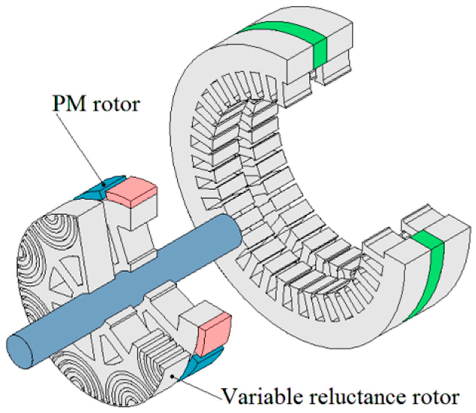
These machines can be considered an integration of a non-salient permanent magnet (PM) rotor and a variable reluctance rotor within the same stator (Figure 1) [6,8].

This contribution builds upon previous research on the power capabilities of SIAPMSMs. However, unlike earlier studies that did not take losses into account [9], it focuses on SIAPMSM models that consider electromagnetic losses (joule and iron losses). This study focuses on investigating the power capability of SIAPMSMs, examining both low-speed operations (maximum torque region) and high-speed operations (flux weakening region). The goal is to validate the newly developed tool by comparing it with previous works dedicated to the power capability of synchronous motors [3,10,11,12,13,14,15] and lossless SIAPMSMs [9]. The newly developed tool also includes electromagnetic losses; it will also be validated against previously developed tools for classical PM machines [13,14,15].

The main novelty of this contribution is the extension of previous works on the power capabilities and efficiency maps of synchronous machines [13,14,15] in the case of SIAPMSMs. Indeed, very few contributions have been dedicated to the efficiency maps of SIAPMSMs [16]. Furthermore, the developed tools are made available to the readers. They can use them to deepen the presented study.

The principle of SIAPMSMs and some structures are introduced in Section 2. In Section 3, the lossless model is presented before the model taking the electromagnetic losses into account is introduced. Section 4 presents the tools developed to investigate the power capability under motoring mode. In addition, the validations of the tools with some analyses and comparisons with the previous tools are also presented in Section 4. Finally, some conclusions and perspectives of the work are presented.

2. Shifted Inductances Axes Permanent Magnet Synchronous Motors (SIAPMSMs)

In order to introduce the principle of SIAPMSMs, it is helpful to represent the context in which this idea is based. It will aid in clarifying how these structures enhance torque capacity in comparison to classical PM machines.

2.1. SIAPMSM Machines Principle

Different SIAPMSM machine structures exist. Some have 3D structures (Figure 1) and some have 2D structures. The design in Figure 1 consists of two axially parallel rotors, a PM rotor, and a variable reluctance rotor. As highlighted in [6], and designed in order to improve the flux-weakening performance, Prof. B. J. Chalmers has proposed the concept of a parallel hybrid rotor design [17,18,19,20]. As is also highlighted in [6], since then, various parallel rotor designs were presented in terms of hybrid excitation structures [21,22].

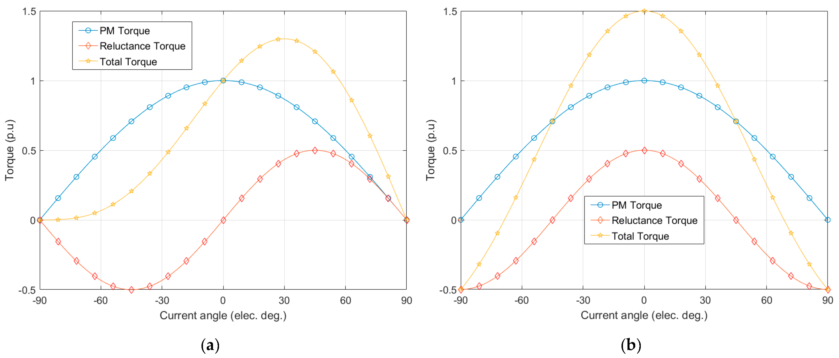
The principle of shifted inductances axis permanent magnet synchronous machines has already been presented in many contributions [4,5,6,7,8]. It consists of aligning the maximum permanent magnet torque and reluctance torque components. Figure 2 illustrates this principle. In these figures (Figure 2), the torques are normalized according to the maximum value of the PM torque component.

.

2.2. SIAPMSM Structures

Some structures presented in the scientific literature are overviewed in this section [4,5,6,7,8]. Various structures of SIAPMSMs can be created [8]; the one depicted in Figure 1 can be considered a quasi-3D structure.

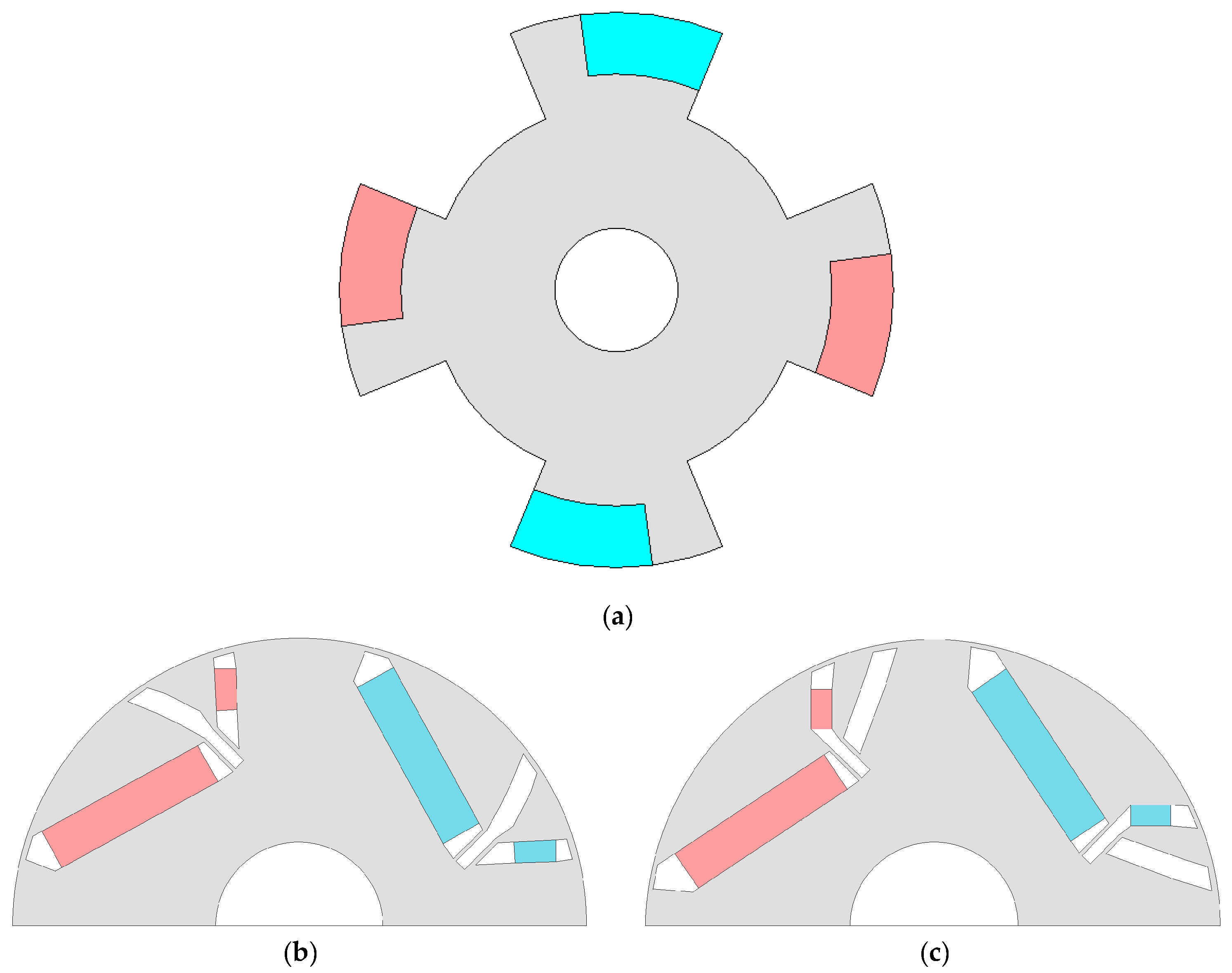
Additionally, several 2D structures of SIAPMSMs are available and some rotor designs are presented in Figure 3. For a comprehensive review of SIAPMSM structures, readers may refer to [8].

3. Modeling of SIAPMSMs

In order to fully understand the principle of SIAPMSMs, a modeling approach based on equivalent electrical circuits is presented. The work starts with the lossless model and then shifts to the model with losses. In this regard, it is useful to note that a power invariant Park transformation is employed to convert the three-phase stationary ABC variables into 0dq variables. It is worth noting that the zero-axis has no effect on the mechanical output power; thus, its study is limited only in terms of the ($d,q$) referential frame.

3.1. Decomposition into Two Machines

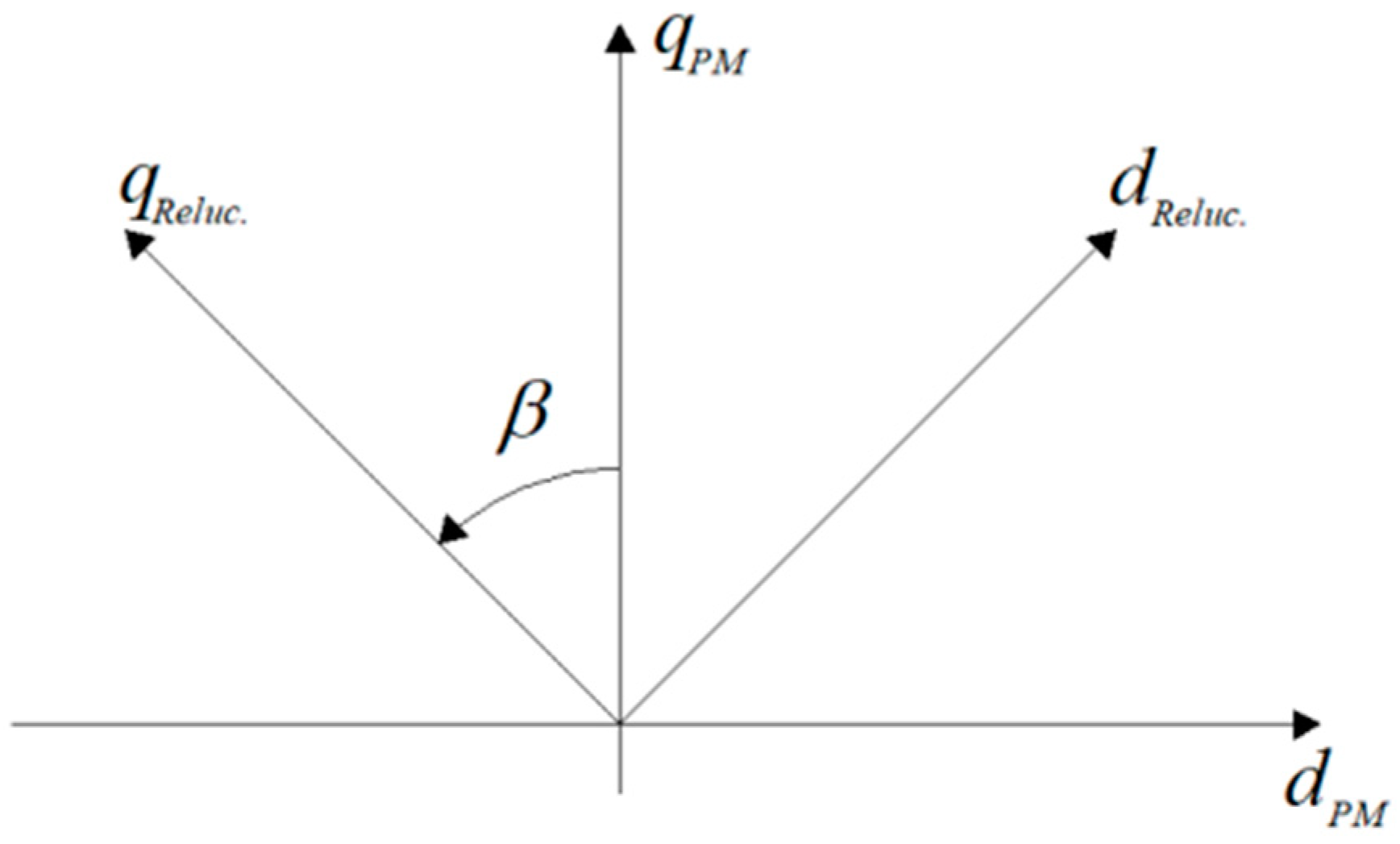
A SIAPMSM can be defined as the combination of two rotors under the same stator, a non-salient PM rotor and a variable reluctance rotor. Two Park’s referential frames can be then defined, one for the non-salient PM rotor part ($d_{PM},q_{PM}$) and a second for the variable reluctance rotor part ($d_{Reluc.},q_{Reluc.}$), shifted by the angle β (Figure 4). The model of a SIAPMSM is defined using the principle of superposition. The $d_{PM}$ axis is defined as the axis of maximum flux linkage and the $d_{Reluc.}$ axis can be chosen as the axis of minimum ($\rho$ < 1) or maximum ($\rho$ > 1) inductance. It is worth mentioning that, for a given value of β, the machine’s characteristics are dependent on the direction of rotation [19].

3.2. Lossless Model

Figure 5 represents the equivalent circuits’ models for shifted inductance axes permanent magnet machines in $(d_{PM},q_{PM})$ or $(d_{Reluc.},q_{Reluc.})$ reference frames.

Relations between the quantities in the two reference frames, $(d_{PM},q_{PM})$ and $(d_{Reluc.},q_{Reluc.})$, are defined by (1):

$$\left\{\begin{array}{c}{f}_{d,qPM}=T_{\beta }{f}_{d,qReluc.}\\ f_{d,qReluc.}={T_{\beta }}^{-1}{f}_{d,qPM}\end{array}\right.,$$

(1)

where $T_{\beta }$ is the transfer matrix defined by:

$$T_{\beta }=\left[\begin{array}{cc}\cos \left(\beta \right)& -\sin \left(\beta \right)\\ \sin \left(\beta \right)& \cos \left(\beta \right)\end{array}\right]\Rightarrow {T_{\beta }}^{-1}=\left[\begin{array}{cc}\cos \left(\beta \right)& \sin \left(\beta \right)\\ -\sin \left(\beta \right)& \cos \left(\beta \right)\end{array}\right].$$

(2)

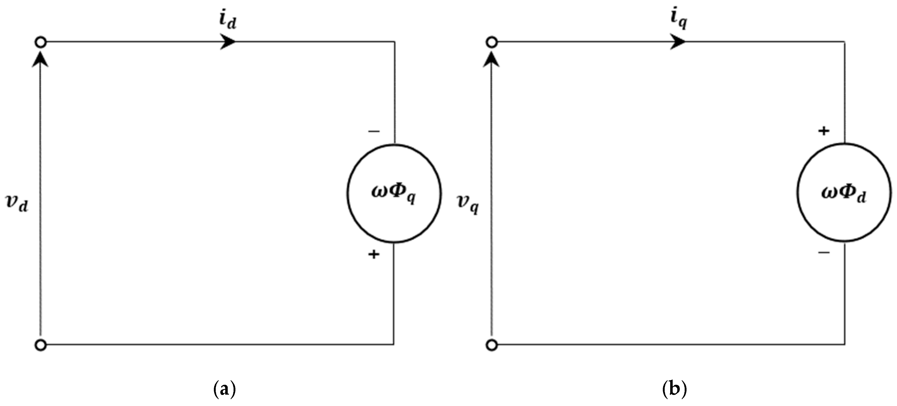
It is worth mentioning that this matrix is orthonormal and it allows for power conservation. The symbols in Figure 5 are defined as:

• Symbols $i_d,i_q$: d and q axes components of armature current;
• Symbols $v_d,v_q$: d and q axes components of terminal voltage;
• Symbols ${\Phi }_d,{\Phi }_q$: d and q axes components of magnetic flux.

3.2.1. Representation in the ${(d}_{PM},q_{PM})$ Referential Frame

The expressions of the armature terminal voltage components for a lossless SIAPMSM in the ${(d}_{PM},q_{PM})$ referential frame are expressed as:

$$\begin{gathered} \left[\genfrac{}{}{0pt}{}{v_d}{v_q}\right]=\omega \left[\genfrac{}{}{0pt}{}{{-\Phi }_q}{{\Phi }_d}\right] \\ =\frac{\omega L_d}{2}\left[\begin{array}{cc}-\left(1-\rho \right)\mathit{sin}\left(2\beta \right)& -\left(1+\rho \right)+\left(1-\rho \right)\mathit{cos}\left(2\beta \right)\\ \left(1+\rho \right)+\left(1-\rho \right)\mathit{cos}\left(2\beta \right)& \left(1-\rho \right)\mathit{sin}\left(2\beta \right)\end{array}\right]\left[\genfrac{}{}{0pt}{}{i_d}{i_q}\right]+\omega {\Phi }_a\left[\genfrac{}{}{0pt}{}{0}{1}\right] \end{gathered}$$

(3)

where $\rho$ is the saliency ratio$(=L_q/L_d)$, with $L_d$ and $L_q$ being the d and q axes components of synchronous inductance; ${\Phi }_a$ is the permanent magnet flux linkage.

The active power P, neglecting the loss, is given by:

$$P=v_d{i}_d+v_q{i}_q=\omega \left[{\Phi }_a{i}_q+\left(L_d-L_q\right)\mathit{cos}\left(2\beta \right)i_d{i}_q+\frac{\left(L_d-L_q\right)}{2}\mathit{sin}\left(2\beta \right)\left({i_q}^2-{i_d}^2\right)\right]$$

(4)

where $\omega (=p\Omega )$ is the electric pulsation ($p$ is the number of pole pairs and $\Omega$ is the rotational mechanical speed).

The equation of the torque is given by:

$$\Gamma =\frac{P}{\Omega }=p\left[{\Phi }_a{i}_q+\left(L_d-L_q\right)\mathit{cos}\left(2\beta \right)i_d{i}_q+\frac{\left(L_d-L_q\right)}{2}\mathit{sin}\left(2\beta \right)\left({i_q}^2-{i_d}^2\right)\right]$$

(5)

By representing the armature current components as:

$$\left\{\begin{array}{c}{i}_d=-I\mathit{sin}\left(\psi \right)\\ i_q=I\mathit{cos}\left(\psi \right)\end{array}\right.$$

(6)

where I is the armature current amplitude and $\psi$ is the phase shift between armature current and electromotive force EMF.

The expressions of the terminal voltage components are given by:

$$\left\{\begin{array}{c}{v}_d=-\frac{\omega }{2}I\left[\left(L_d+L_q\right)\mathit{cos}\left(\psi \right)-\left(L_d-L_q\right)\mathit{cos}\left(\psi -2\beta \right)\right]\\ v_q=\omega \left[{\Phi }_a-\frac{I}{2}\left(\left(L_d+L_q\right)\mathit{sin}\left(\psi \right)+\left(L_d-L_q\right)\mathit{sin}\left(\psi -2\beta \right)\right)\right]\end{array}\right.$$

(7)

The active power expression becomes:

$$P=\omega \left[{\Phi }_{a}I\mathit{cos}\left(\psi \right)-\frac{I^2}{2}\left(L_d-L_q\right)\mathit{sin}\left(2(\psi -\beta )\right)\right]$$

(8)

The torque $\Gamma$ expression is then:

$$\Gamma =p\left[{\Phi }_{a}I\mathit{cos}\left(\psi \right)-\frac{I^2}{2}\left(L_d-L_q\right)\mathit{sin}\left(2(\psi -\beta )\right)\right]$$

(9)

3.2.2. Representation in the ${(d}_{Reluc.},q_{Reluc.})$ Referential Frame

In the ${(d}_{Reluc.},q_{Reluc.})$ referential frame, the expressions of the armature terminal voltages components are given by:

$$\left[\genfrac{}{}{0pt}{}{v_d}{v_q}\right]=\omega \left[\genfrac{}{}{0pt}{}{{-\Phi }_q}{{\Phi }_d}\right]=\omega L_d\left[\begin{array}{cc}0& -\rho \\ 1& 0\end{array}\right]\left[\genfrac{}{}{0pt}{}{i_d}{i_q}\right]+\omega {\Phi }_a\left[\genfrac{}{}{0pt}{}{\mathit{sin}\left(\beta \right)}{\mathit{cos}\left(\beta \right)}\right]$$

(10)

The active power P is given by:

$$P=v_d{i}_d+v_q{i}_q=\omega \left[{\Phi }_a\left(\mathit{sin}\left(\beta \right)i_d+\mathit{cos}\left(\beta \right)i_q\right)+\left(L_d-L_q\right)i_d{i}_q\right]$$

(11)

The equation of the torque results is given by:

$$\Gamma =p\left[{\Phi }_{\mathrm{a}}\left(\mathit{sin}\left(\beta \right)i_d+\mathit{cos}\left(\beta \right)i_q\right)+\left(L_d-L_q\right)i_d{i}_q\right]$$

(12)

Considering the armature current components:

$$\left\{\begin{array}{c}{i}_d=-I\mathit{sin}\left(\psi -\beta \right)\\ i_q=I\mathit{cos}\left(\psi -\beta \right)\end{array}\right.$$

(13)

The expression of the terminal voltage components is given by:

$$\left\{\begin{array}{c}{v}_d=\omega {\Phi }_{\mathrm{a}}\mathit{sin}\left(\beta \right)-I\omega L_q\mathit{cos}\left(\psi -\beta \right)\\ v_q=\omega {\Phi }_{\mathrm{a}}\mathit{cos}\left(\beta \right)-I\omega L_d\mathit{sin}\left(\psi -\beta \right)\end{array}\right.$$

(14)

Since a power invariant transformation is used, the active power and the torque expressions are identical to those of the ${(d}_{PM},q_{PM})$ referential frame.

On the other hand, using the relations of Equations (1) and (2), the expression of the power in the ${(d}_{Reluc.},q_{Reluc.})$ referential frame is:

$$\begin{gathered} P_{Reluc.}={v_{Reluc.}}^T·i_{Reluc.}={\left(\genfrac{}{}{0pt}{}{v_{dReluc.}}{v_{qReluc.}}\right)}^T·\left(\genfrac{}{}{0pt}{}{i_{dReluc.}}{i_{qReluc.}}\right)={\left({T_{\beta }}^{-1}·\left(\genfrac{}{}{0pt}{}{v_{dPM}}{v_{qPM}}\right)\right)}^T·{T_{\beta }}^{-1}·\left(\genfrac{}{}{0pt}{}{i_{dPM}}{i_{qPM}}\right) \\ ={v_{PM}}^T·{\left({T_{\beta }}^{-1}\right)}^T·{T_{\beta }}^{-1}·i_{PM}={v_{PM}}^T·T_{\beta }·{T_{\beta }}^{-1}·i_{PM}={v_{PM}}^T·I_{2x2}·i_{PM}=P_{PM} \end{gathered}$$

(15)

Similarly:

$$\left\{\begin{array}{c}{V_{Reluc.}}^2={V_{Reluc.}}^T·V_{Reluc.}={V_{PM}}^T·V_{PM}={V_{PM}}^2\\ {I_{Reluc.}}^2={I_{Reluc.}}^T·I_{Reluc.}={I_{PM}}^T·I_{PM}={I_{PM}}^2\end{array}\right.$$

(16)

with V and I being the voltage and current amplitudes.

So, finally, it is clear that the study of the power capability in the reference frames ${(d}_{PM},q_{PM})$ and ${(d}_{Reluc.},q_{Reluc.})$ gives the same results.

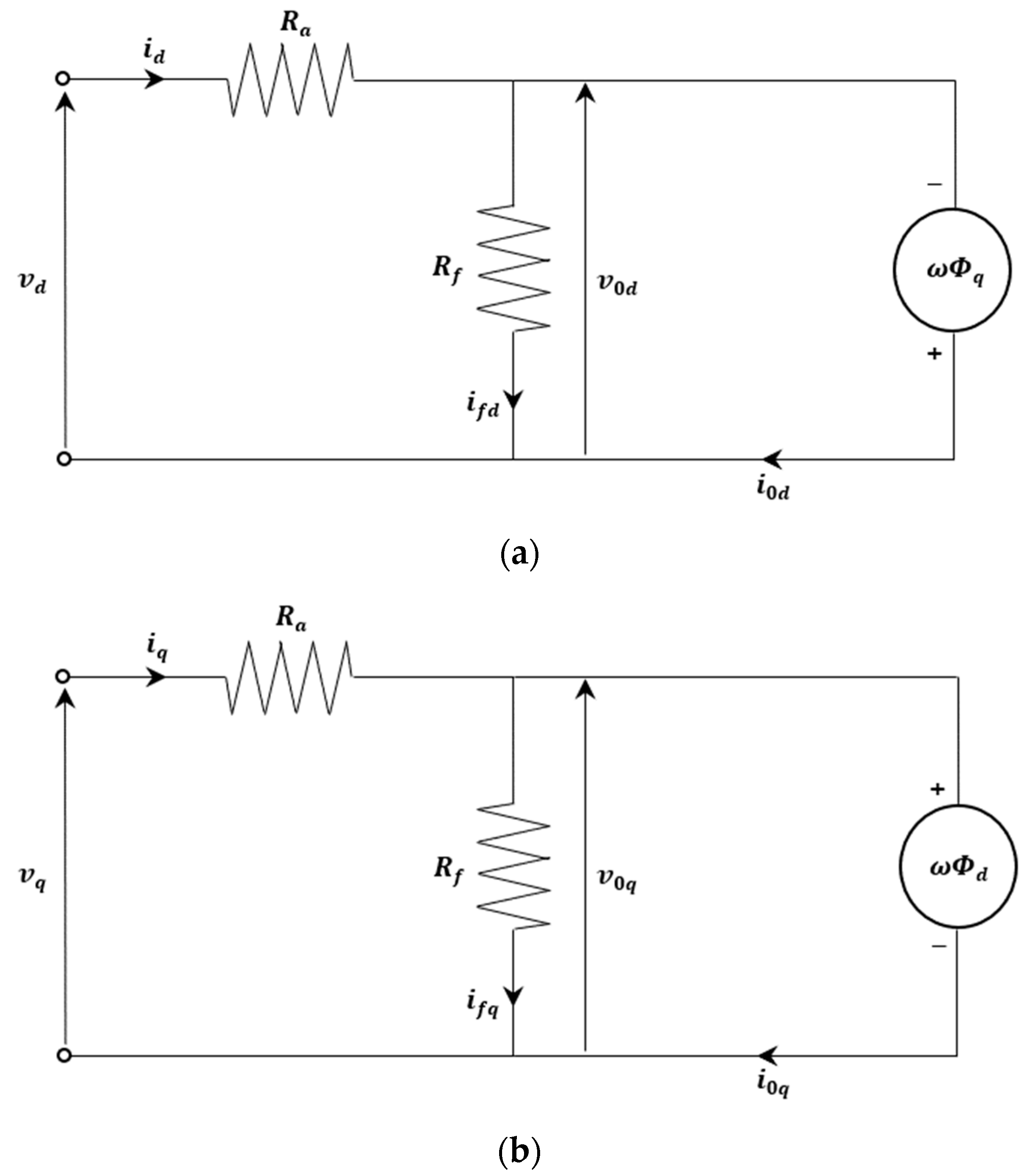
3.3. Model including the Electromagnetic Losses

In order to consider the electromagnetic losses, first resistance is added in parallel with the lossless model. This resistance represents iron loss. A second resistance is then added in series with the circuit corresponding to the paralleling of the iron loss resistance and the lossless model circuits. The second resistance represents the joule losses. Figure 6 shows the equivalent electric circuit models, including these resistances [23,24,25].

The new symbols in Figure 6 are defined as:

• Symbols $i_{fd},i_{fq}$: d and q axes components of iron loss current;
• Symbols $R_a$: armature winding resistance per phase;
• Symbols $R_f$: iron loss resistance.

From Figure 6, the armature voltage equations in both referential frames can be expressed as:

$$\left[\genfrac{}{}{0pt}{}{v_d}{v_q}\right]=R_a\left[\genfrac{}{}{0pt}{}{i_d}{i_q}\right]+\left[\genfrac{}{}{0pt}{}{v_{0d}}{v_{0q}}\right],$$

(17)

where,

$$i_d=i_{0d}+i_{fd}=i_{0d}+\frac{v_{0d}}{R_f}$$

(18)

$$i_q=i_{0q}+i_{fq}=i_{0q}+\frac{v_{0q}}{R_f}$$

(19)

In following subsections, the model including the losses is presented in the two referential frames ${(d}_{PM},q_{PM})$ and ${(d}_{Reluc.},q_{Reluc.})$.

3.3.1. Representation in the ${(d}_{PM},q_{PM})$ Referential Frame

The components $v_{0d}$ and $v_{0q}$ in the ${(d}_{PM},q_{PM})$ referential frame can be expressed as:

$$\left[\genfrac{}{}{0pt}{}{v_{0d}}{v_{0q}}\right]=\frac{\omega L_d}{2}\left[\begin{array}{cc}-\left(1-\rho \right)\mathit{sin}\left(2\beta \right)& -\left(1+\rho \right)+\left(1-\rho \right)\mathit{cos}\left(2\beta \right)\\ \left(1+\rho \right)+\left(1-\rho \right)\mathit{cos}\left(2\beta \right)& \left(1-\rho \right)\mathit{sin}\left(2\beta \right)\end{array}\right]\left[\genfrac{}{}{0pt}{}{i_{0d}}{i_{0q}}\right]+\omega {\Phi }_a\left[\genfrac{}{}{0pt}{}{0}{1}\right]$$

(20)

Considering the electromagnetic losses, the total active power is given by:

$$\begin{array}{cc}\hfill P_{Total}& =v_d{i}_d+v_q{i}_q=P_{Cu}+P_{Fe}+P_{out}\hfill \\ \hfill & =\mathrm{c}\mathrm{o}\mathrm{p}\mathrm{p}\mathrm{e}\mathrm{r}\mathrm{l}\mathrm{o}\mathrm{s}\mathrm{s}\mathrm{e}\mathrm{s}+\mathrm{i}\mathrm{r}\mathrm{o}\mathrm{n}\mathrm{l}\mathrm{o}\mathrm{s}\mathrm{s}\mathrm{e}\mathrm{s}+\mathrm{m}\mathrm{e}\mathrm{c}\mathrm{h}\mathrm{a}\mathrm{n}\mathrm{i}\mathrm{c}\mathrm{a}\mathrm{l}\mathrm{o}\mathrm{u}\mathrm{t}\mathrm{p}\mathrm{u}\mathrm{t}\mathrm{p}\mathrm{o}\mathrm{w}\mathrm{e}\mathrm{r}\hfill \end{array}$$

(21)

The mechanical output power is given by:

$$\begin{array}{cc}\hfill P_{out}& =v_{0d}{i}_{0d}+v_{0q}{i}_{0q}\hfill \\ \hfill & =\omega \left[{\Phi }_a{i}_{0q}+\left(1-\rho \right)L_d\mathit{cos}\left(2\beta \right)i_{0d}{i}_{0q}+\frac{\left(1-\rho \right)L_d}{2}\mathit{sin}\left(2\beta \right)\left({i_{0q}}^2-{i_{0d}}^2\right)\right]\hfill \end{array}$$

(22)

Then, the torque expression is given by:

$$\Gamma =\frac{P_{out}}{\Omega }=p\left[{\Phi }_a{i}_{0q}+\left(1-\rho \right)L_d\mathit{cos}\left(2\beta \right)i_{0d}{i}_{0q}+\frac{\left(1-\rho \right)L_d}{2}\mathit{sin}\left(2\beta \right)\left({i_{0q}}^2-{i_{0d}}^2\right)\right]$$

(23)

From Equations (18)–(20), it is possible to determine the relations between components ${(i}_{0d},i_{0q})$ and ${(i}_d,i_q)$:

$$\left[\genfrac{}{}{0pt}{}{i_{0d}}{i_{0q}}\right]=\frac{1}{∆}\left[\begin{array}{cc}{A}_{PM}& B_{PM}\\ C_{PM}& D_{PM}\end{array}\right]\left[\genfrac{}{}{0pt}{}{i_d}{i_q-\frac{\omega {\Phi }_a}{R_f}}\right],$$

(24)

with,

$$∆=1+\rho {\left(\frac{\omega L_d}{R_f}\right)}^2,$$

$$A_{PM}=1+\frac{\omega L_d}{{2R}_f}\left(1-\rho \right)\sin \left(2\beta \right),$$

$$B_{PM}=\frac{\omega L_d}{{2R}_f}\left(\left(1+\rho \right)-\left(1-\rho \right)\cos \left(2\beta \right)\right),$$

$$C_{PM}=-\frac{\omega L_d}{{2R}_f}\left(\left(1+\rho \right)+\left(1-\rho \right)\cos \left(2\beta \right)\right),$$

$$D_{PM}=1-\frac{\omega L_d}{{2R}_f}\left(1-\rho \right)\sin \left(2\beta \right).$$

From Equations (6), (22)–(24), it is possible to express the output power and torque in the function of the armature current amplitude:

$$P_{\mathrm{o}\mathrm{u}\mathrm{t}}=\frac{\omega }{{∆}^2}\left[A_1{I}^2+B_{1}I+C_1\right],$$

(25)

$$\Gamma =\frac{P_{out}}{\Omega }=\frac{p}{{∆}^2}\left[A_1{I}^2+B_{1}I+C_1\right],$$

(26)

with,

$$A_1=\frac{\left(1-\rho \right)L_d}{2}\left(\frac{\omega L_d}{R_f}\left(\left(1+\rho \right)\mathit{cos}\left(2\left(\psi -\beta \right)\right)-\left(1-\rho \right)\right)-\left(1-\rho {\left(\frac{\omega L_d}{R_f}\right)}^2\right)\mathit{sin}\left(2\left(\psi -\beta \right)\right)\right),$$

$$\begin{gathered} B_1={\Phi }_a\left(\frac{\omega L_d}{R_f}\left(\left(1+\rho {\left(\frac{\omega L_d}{R_f}\right)}^2\right)\frac{\left(1+\rho \right)}{2}\mathit{sin}\left(\psi \right)+\left(3-\rho {\left(\frac{\omega L_d}{R_f}\right)}^2\right)\frac{\left(1-\rho \right)}{2}\mathit{sin}\left(\psi -2\beta \right) \\ -\left(1-{\rho }^2\right)\frac{\omega L_d}{R_f}\mathit{cos}\left(\psi -2\beta \right)\right)+\left(1+\left(1-\rho +{\rho }^2\right){\left(\frac{\omega L_d}{R_f}\right)}^2\right)\mathit{cos}\left(\psi \right)\right), \end{gathered}$$

$$C_1=\frac{{{\Phi }_a}^2}{R_f}\omega \left(\frac{\omega L_d}{R_f}\left(1-\rho \right)\mathit{sin}\left(2\beta \right)+\frac{\left(1-{\rho }^2\right)}{2}{\left(\frac{\omega L_d}{R_f}\right)}^2\mathit{cos}\left(2\beta \right)-\left(1+\frac{\left(1+{\rho }^2\right)}{2}{\left(\frac{\omega L_d}{R_f}\right)}^2\right)\right).$$

It is worth mentioning that by eliminating the losses from this model, by setting $R_a=0\mathsf{\Omega }\mathrm{a}\mathrm{n}\mathrm{d}{R}_f=+\infty \mathsf{\Omega }$, the expressions of power and torque coincide with those of the lossless model. Furthermore, by imposing $\beta$ to zero, the model with the losses coincides with the model of the classic PM machines with losses [13,14].

3.3.2. Representation in the ${(d}_{Reluc.},q_{Reluc.})$ Referential Frame

The components $v_{0d}$ and $v_{0q}$ in the ${(d}_{Reluc.},q_{Reluc.})$ referential frame can be expressed as:

$$\left[\genfrac{}{}{0pt}{}{v_{0d}}{v_{0q}}\right]=\omega L_d\left[\begin{array}{cc}0& -\rho \\ 1& 0\end{array}\right]\left[\genfrac{}{}{0pt}{}{i_{0d}}{i_{0q}}\right]+\omega {\Phi }_a\left[\genfrac{}{}{0pt}{}{\mathit{sin}\left(\beta \right)}{\mathit{cos}\left(\beta \right)}\right]$$

(27)

The expression of the total active power given by Equation (21) is still valid in the ${(d}_{Reluc.},q_{Reluc.})$ referential frame. The mechanical output power is given by:

$$P_{out}=v_{0d}{i}_{0d}+v_{0q}{i}_{0q}=\omega \left[{\Phi }_a\left(\mathit{sin}\left(\beta \right)i_{0d}+\mathit{cos}\left(\beta \right)i_{0q}\right)+\left(1-\rho \right)L_d{i}_{0d}{i}_{0q}\right]$$

(28)

Then, the torque expression is given by:

$$\Gamma =\frac{P_{out}}{\Omega }=p\left[{\Phi }_a\left(\mathit{sin}\left(\beta \right)i_{0d}+\mathit{cos}\left(\beta \right)i_{0q}\right)+\left(1-\rho \right)L_d{i}_{0d}{i}_{0q}\right]$$

(29)

From Equations (18), (19), and (27), it is possible to determine the relations between components ${(i}_{0d},i_{0q})$ and ${(i}_d,i_q)$:

$$\left[\genfrac{}{}{0pt}{}{i_{0d}}{i_{0q}}\right]=\frac{1}{∆}\left[\begin{array}{cc}{A}_{Reluc.}& B_{Reluc.}\\ C_{Reluc.}& D_{Reluc.}\end{array}\right]\left[\genfrac{}{}{0pt}{}{i_d-\frac{\omega {\Phi }_a}{R_f}\left(\mathit{sin}\left(\beta \right)+\rho \frac{\omega L_d}{R_f}\mathit{cos}\left(\beta \right)\right)}{i_q-\frac{\omega {\Phi }_a}{R_f}\left(\mathit{cos}\left(\beta \right)-\frac{\omega L_d}{R_f}\mathit{sin}\left(\beta \right)\right)}\right],$$

(30)

with,

$$∆=1+\rho {\left(\frac{\omega L_d}{R_f}\right)}^2,$$

$$A_{Reluc.}=1,$$

$$B_{Reluc.}=\rho \frac{\omega L_d}{R_f},$$

$$C_{Reluc.}=-\frac{\omega L_d}{R_f},$$

$$D_{Reluc.}=1.$$

Seeking to express the output power and torque in the function of the armature current amplitude from Equations (28)–(30), the same equations as (25) and (26) are respectively obtained. Again, the power is conserved whether expressed in the ${(d}_{Reluc.},q_{Reluc.})$ referential frame or the ${(d}_{PM},q_{PM})$ referential frame.

3.4. Per-Unit System

The per-unit system model facilitates a deeper comprehension of how parameters impact machine performance, enabling the derivation of general conclusions regarding the power capability of these motors. Furthermore, it serves as a powerful tool for the classification of electric machine drives [10,12,26]. At rated speed (base speed ${\Omega }_b$), the base values of EMF $\left(p{\Phi }_a{\Omega }_b\right)$ and armature current $\left(I_m\right)$ are chosen as the rated values of the motor.

The per-unit values of the resistances and inductances are defined as:

$$R_{an}=\frac{R_a{I}_m}{{\Phi }_{a}p{\Omega }_b},R_{fn}=\frac{R_f{I}_m}{{\Phi }_{a}p{\Omega }_b},$$

(31)

$$L_{dn}=\frac{L_d{I}_m}{{\Phi }_a},L_{qn}=\rho L_{dn}.$$

(32)

It should be noticed that $I_m$ is the rated amplitude in the $(d,q)$ referential frame. The subscript n indicates the per-unit value.

The per-unit values of the armature currents and the armature terminal voltage are given by:

$$I_n=\frac{\sqrt{I_d^2+I_q^2}}{I_m},V_n=\frac{\sqrt{v_d^2+v_q^2}}{{\Phi }_{a}p{\Omega }_b},$$

(33)

In addition, the per-unit values of output power $P_{out}$, copper loss $P_{Cu}$, and iron loss $P_{Fe}$ are given by:

$$P_{outn}=\frac{P_{out}}{V_m{I}_m},P_{Cun}=\frac{P_{Cu}}{V_m{I}_m},P_{Fen}=\frac{P_{Fe}}{V_m{I}_m},$$

(34)

where $V_m$ is the maximum (rated) armature terminal voltage amplitude in the $(d,q)$ referential frame.

Finally, the per-unit values of the speed and torque are defined as:

$${\Omega }_n=\frac{\Omega }{{\Omega }_b},{\Gamma }_n=\frac{P_{outn}}{{\Omega }_n}.$$

(35)

It should be noticed that the normalized power defined in Equation (34) corresponds to the power factor for the lossless model. This is also the case for the normalised torque, as defined in Equation (35) at the base speed.

Having defined the normalization bases, it worth defining the normalized value of torque:

$${\Gamma }_n=\frac{1}{{V_{nmax}.{∆}_n}^2}\left[A_{1n}{I_n}^2+B_{1n}{I}_n+C_{1n}\right],$$

(36)

with,

$${∆}_n=∆=1+\rho {\left(\frac{{\mathsf{\Omega }}_n{L}_{dn}}{R_{fn}}\right)}^2,$$

$$A_{1n}=\frac{\left(1-\rho \right)L_{dn}}{2}\left(\frac{{\mathsf{\Omega }}_n{L}_{dn}}{R_{fn}}\left(\left(1+\rho \right)\mathit{cos}\left(2\left(\psi -\beta \right)\right)-\left(1-\rho \right)\right)-\left(1-\rho {\left(\frac{{\mathsf{\Omega }}_n{L}_{dn}}{R_{fn}}\right)}^2\right)\mathit{sin}\left(2\left(\psi -\beta \right)\right)\right),$$

$$\begin{gathered} B_{1n}=\frac{{\mathsf{\Omega }}_n{L}_{dn}}{R_{fn}}\left(\left(1+\rho {\left(\frac{{\mathsf{\Omega }}_n{L}_{dn}}{R_{fn}}\right)}^2\right)\frac{\left(1+\rho \right)}{2}\mathit{sin}\left(\psi \right)+\left(3-\rho {\left(\frac{{\mathsf{\Omega }}_n{L}_{dn}}{R_{fn}}\right)}^2\right)\frac{\left(1-\rho \right)}{2}\mathit{sin}\left(\psi -2\beta \right) \\ -\left(1-{\rho }^2\right)\left(\frac{{\mathsf{\Omega }}_n{L}_{dn}}{R_{fn}}\right)\mathit{cos}\left(\psi -2\beta \right)\right)+\left(1+\left(1-\rho +{\rho }^2\right){\left(\frac{{\mathsf{\Omega }}_n{L}_{dn}}{R_{fn}}\right)}^2\right)\mathit{cos}\left(\psi \right), \end{gathered}$$

$$C_{1n}=\frac{{\mathsf{\Omega }}_n}{R_{fn}}\left(\left(\frac{{\mathsf{\Omega }}_n{L}_{dn}}{R_{fn}}\right)\left(1-\rho \right)\mathit{sin}\left(2\beta \right)+\frac{\left(1-{\rho }^2\right)}{2}{\left(\frac{{\mathsf{\Omega }}_n{L}_{dn}}{R_{fn}}\right)}^2\mathit{cos}\left(2\beta \right)-\left(1+\frac{\left(1+{\rho }^2\right)}{2}{\left(\frac{{\mathsf{\Omega }}_n{L}_{dn}}{R_{fn}}\right)}^2\right)\right).$$

4. Efficiency Maps of SIAPMSMs

The efficiency map estimation discussed in this contribution is produced for optimal control, allowing for maximizing the efficiency while respecting the current and voltage limits constraints.

The study discussed in this contribution relies on the work presented in [13,14,15]. The newly developed algorithm, presented in this contribution, constitutes the main novelty in the sense that it is more general than previously developed algorithms. Readers are invited to access the MATLAB scripts allowing for the estimation of the efficiency maps for these machines through the link given as reference [27].

Due to complicated equations, the analytical developments are limited and most of the steps allowing for the determination of the triple $(I,\psi ,\beta )$ maximizing of the efficiency are processed numerically. The previous cases (lossless classical PM motor, lossless SIAPMSM, and classical PM motor with losses) could be regarded as particular cases of these more general developments. Results from the previous developments, that have been assessed are exploited to assess the validity of these more general developments.

4.1. Presentation of Developed Tool

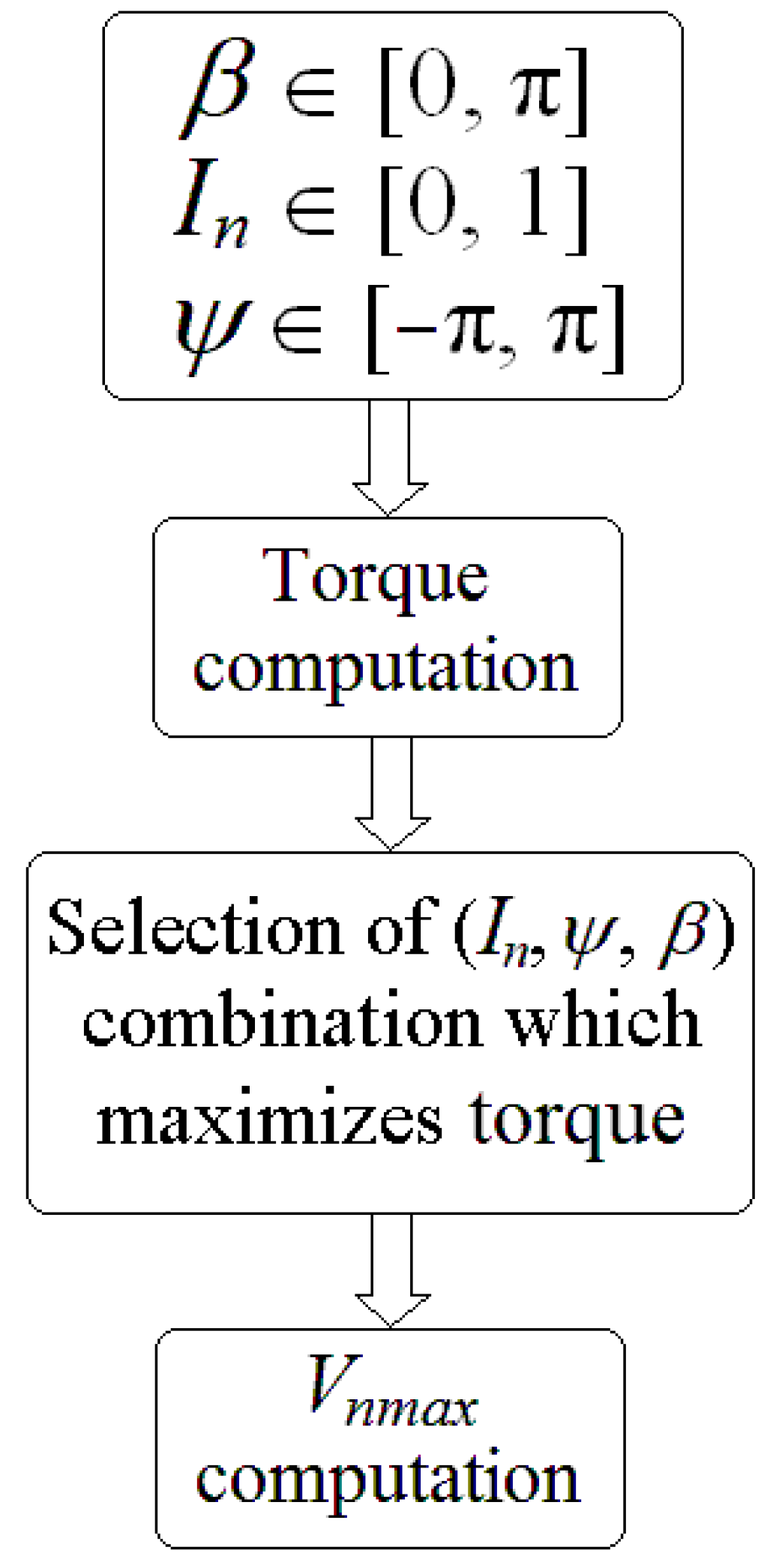
The calculation of $V_{nmax}$, the normalized value of armature windings terminals maximum voltage, constitutes the initial step towards the determination of efficiency maps. This corresponds with the determination of the base speed ${\Omega }_b$. Algorithm 1 represents the MATLAB scripts used in order to determine the value of $V_{nmax}$ for a SIAPMSM with losses as a general structure.

The $h\left(I_n,\psi ,\beta \right)$ function shown in Algorithm 1 is the expression of normalized torque, with respect to PM torque $\left(p{\Phi }_a{I}_m\right)$. As result, this script gives, for each $(L_{dn},\rho )$ couple, the optimal values of $\left(I_{nOpt},{\psi }_{Opt},{\beta }_{Opt}\right)$, which maximizes the torque (Figure 7). For the lossless model, Appendix A presents the analytical developments allowing for the determination of $\left(I_{nOpt},{\psi }_{Opt},{\beta }_{Opt}\right)$ values. Note that, in this case (lossless model), ${\psi }_{Opt}$ is imposed as being equal to zero (${\psi }_{Opt}=0$).

It should be noticed that in all conducted simulations, the highest torque values were always achieved for the maximum armature current $I_m(I_n=1)$. Despite the fact that there is a direct relationship between torque and armature current, this feature has not been confirmed through the analytical model in the general case including the losses.

Algorithm 1. MATLAB script for the determination of $V_{nmax}$.
$\mathbf{S}\mathbf{t}\mathbf{a}\mathbf{r}\mathbf{t}$
$\mathrm{V}\mathrm{a}\mathrm{l}\mathrm{u}\mathrm{e}\mathrm{s}\mathrm{o}\mathrm{f}{L}_{dn},\rho ,R_{an}\mathrm{a}\mathrm{n}\mathrm{d}{R}_{fn}\mathrm{s}\mathrm{h}\mathrm{o}\mathrm{u}\mathrm{l}\mathrm{d}\mathrm{h}\mathrm{a}\mathrm{v}\mathrm{e}\mathrm{b}\mathrm{e}\mathrm{e}\mathrm{n}\mathrm{d}\mathrm{e}\mathrm{f}\mathrm{i}\mathrm{n}\mathrm{e}\mathrm{d};$
$I_n=[0:∆I_n:1];$
$\psi =[-\pi :∆\psi :\pi ];$
$\beta =[0:∆\beta :\pi ];$
$Fori=1:length\left(I_n\right);$
	$Forj=1:length\left(\psi \right)$
		$Fork=1:length\left(\beta \right)$
			${\Gamma }_n^{\prime }\left(k\right)=h\left(I_n\left(i\right),\psi \left(j\right),\beta \left(k\right)\right);\left[\mathrm{s}\mathrm{e}\mathrm{e}\mathrm{E}\mathrm{q}\mathrm{u}\mathrm{a}\mathrm{t}\mathrm{i}\mathrm{o}\mathrm{n}\left(36\right)\right]$
		$End$
		$\left[Y1\left(j\right),X1\left(j\right)\right]=max\left({\Gamma }_n^{\prime }\right);$
		${\Gamma }_{n1}^{\prime }\left(j\right)={\Gamma }_n^{\prime }\left(X1\left(j\right)\right);$
		${\beta }_1\left(j\right)=\beta \left(X1\left(j\right)\right);$
	$End$
	$\left[Y2\left(i\right),X2\left(i\right)\right]=max\left({\Gamma }_{n1}^{\prime }\right);$
	${\Gamma }_{n2}^{\prime }\left(i\right)={\Gamma }_{n1}^{\prime }\left(X2\left(i\right)\right);$
	${\beta }_2\left(i\right)={\beta }_1\left(X2\left(i\right)\right);$
	${\psi }_1\left(i\right)=\psi \left(X2\left(i\right)\right);$
$End$
$\left[Y3,X3\right]=max\left({\Gamma }_{n2}^{\prime }\right);$
$I_{nOpt}=I_n\left(X3\right);$
${\psi }_{Opt}={\psi }_1\left(X3\right);$
${\beta }_{Opt}={\beta }_2\left(X3\right);$
$V_{nmaxd}=f\left(I_{nOpt},{\psi }_{Opt},{\beta }_{Opt}\right);\left[\mathrm{s}\mathrm{e}\mathrm{e}\mathrm{E}\mathrm{q}\mathrm{u}\mathrm{a}\mathrm{t}\mathrm{i}\mathrm{o}\mathrm{n}\left(17\right)\right]$
$V_{nmaxq}=g(I_{nOpt},{\psi }_{Opt},{\beta }_{Opt});[\mathrm{s}\mathrm{e}\mathrm{e}\mathrm{E}\mathrm{q}\mathrm{u}\mathrm{a}\mathrm{t}\mathrm{i}\mathrm{o}\mathrm{n}(17)]$
$V_{nmax}=\mathrm{s}\mathrm{q}\mathrm{r}\mathrm{t}(V_{nmaxd}^2+V_{nmaxq}^2);$
$\mathbf{E}\mathbf{n}\mathbf{d}$

By using the normalized form of the torque in Equation (36), it is possible to derive a second-order polynomial of the normalized current amplitude in Equation (37).

$$A.{I_n}^2+B.I_n+C=0,$$

(37)

where ${A=A}_{1n},B=B_{1n}\mathrm{a}\mathrm{n}\mathrm{d}C=C_{1n}-{\Gamma }_n.{V_{nmax}.{∆}_n}^2$.

For a given $({\Omega }_{\mathrm{n}},{\Gamma }_n,\psi )$ set, if Equation (37) does not have a solution $(∆<0)$, the efficiency is set to null $\eta =0$. In case solutions exist, the current limit constraint $(I_{\mathrm{n}}\le 1)$ and the voltage limit constraint ($V_n\le V_{nmax}$) both have to be respected, otherwise the efficiency is set to null $\eta =0$. In case Equation (37) has two solutions and both allow for respecting the current and voltage limit constraints; the one allowing for maximizing the efficiency is retained.

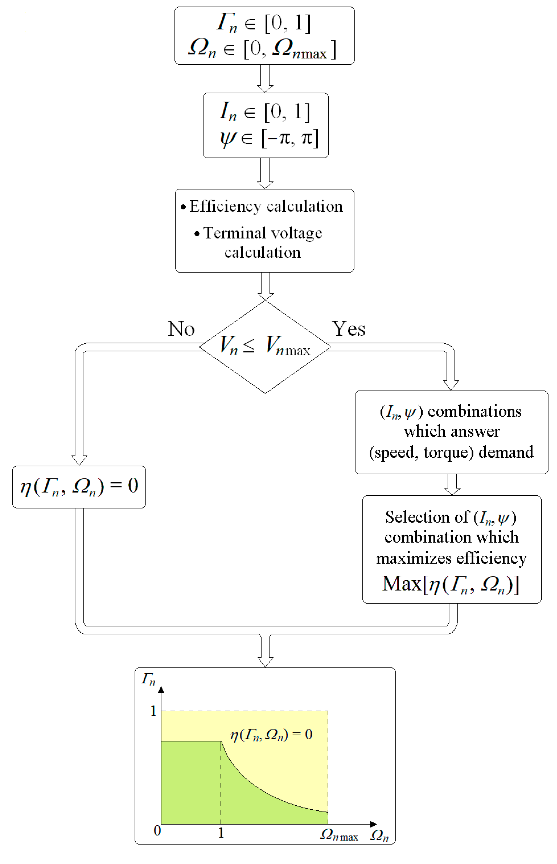
Figure 8 shows the algorithms used to calculate the efficiency maps. The algorithm allows for determining the ${(I}_n,\psi )$ couple maximizing regarding the efficiency for each operating point $({\Omega }_{\mathrm{n}},{\Gamma }_n)$. For lossless synchronous machines, the efficiency of all $({\Omega }_{\mathrm{n}},{\Gamma }_n)$ couples for which it is possible to find couples ($I_n,\psi$) answering the demand while respecting at the same time the current and voltage constraints is set equal to one. For the lossless model, the algorithm does not help to determine the efficiency maps; it is used to determine the envelopes corresponding to the maximum power capability, which is the border between $({\Omega }_{\mathrm{n}},{\Gamma }_n)$ couples for which the efficiency is respectively equal to 0 and 1.

The following step in this work is the validation of the algorithm and the subsequent developed codes [27].

4.2. Validation of Developed Tool

In this section, the newly developed codes are assessed against previous codes. First, the lossless case is considered (Section 4.2.1). The contribution of SIAPMSMs is highlighted in this section. Then, in Section 4.2.2, the model including the electromagnetic losses is assessed.

Table 1. Normalized quantities’ and parameters’ variation intervals.

Quantities and Parameter	Variation Interval
${\Omega }_n$	[0, +∞)
${\Gamma }_n$	[0, 1]
$I_n$	[0, 1]
$L_{dn}$	(0, +∞)
$\rho$	(0, +∞)
$R_{an}$	[0, 10]
$R_{fn}$	(0, +∞)

presents variation intervals for some normalized quantities and parameters. Several references have been analyzed in order to establish reasonable variations intervals of the different quantities and parameters [15,26].

4.2.1. Validation of Developed Tool for the Lossless Case

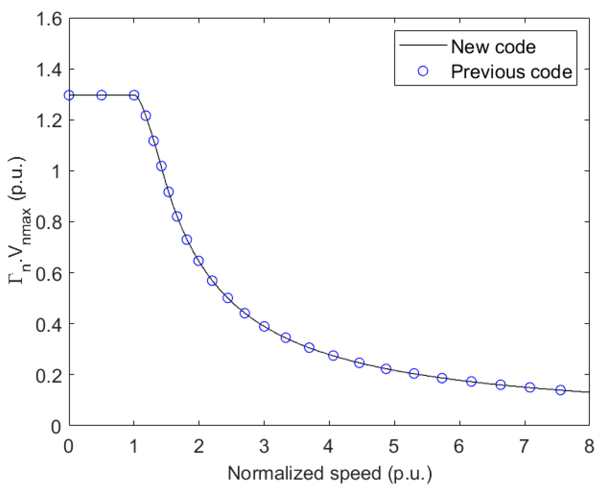
The newly developed codes [27] are first assessed in the lossless case ($R_a=0\mathsf{\Omega }\mathrm{a}\mathrm{n}\mathrm{d}{R}_f=+\infty \mathsf{\Omega }$). Figure 9 compares maximum power capabilities, for a machines with $(L_{dn}=2.5, \rho =0.6)$, obtained using the new codes and previously developed codes [3,9]. As can be seen, good agreement is achieved. The results from the new and old codes have also been compared to other values of $(L_{dn},\rho )$ couples and good agreement was always achieved (curves are matching).

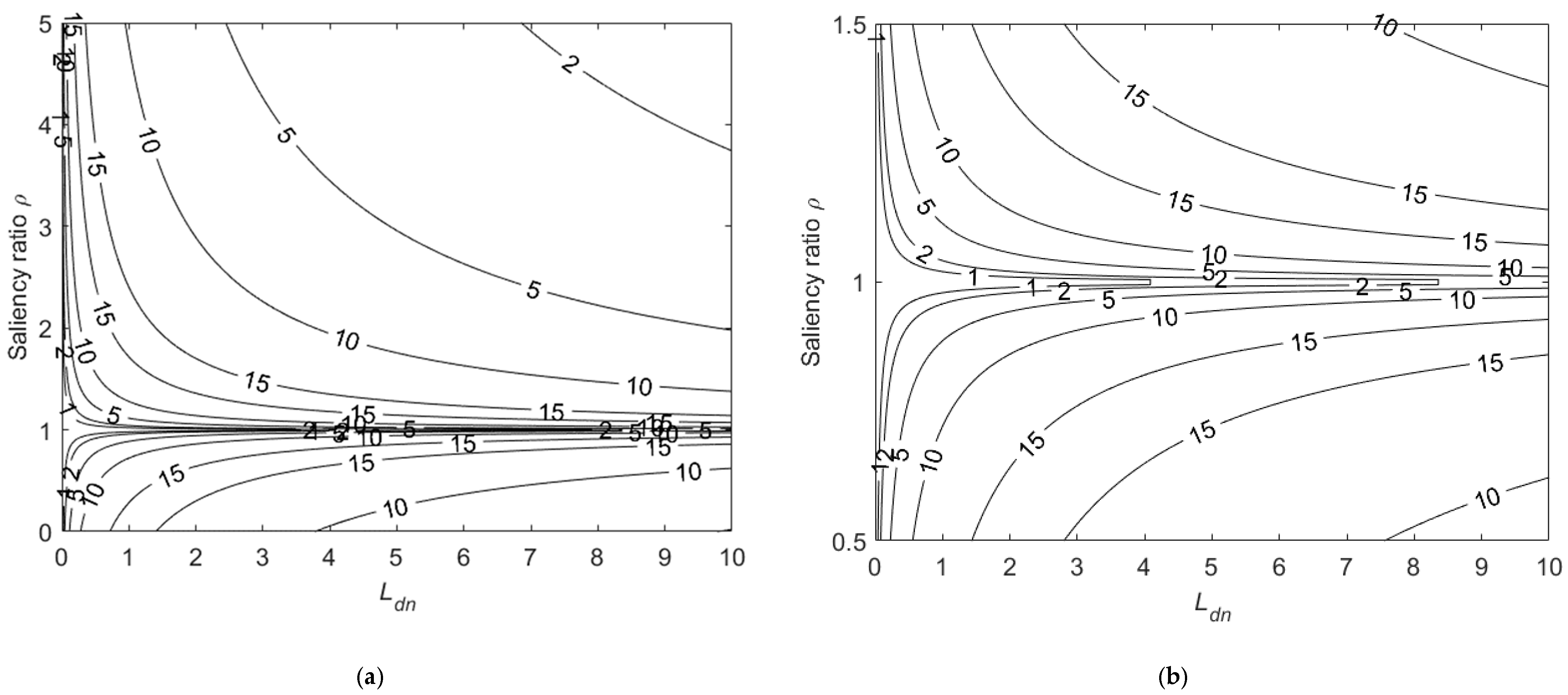
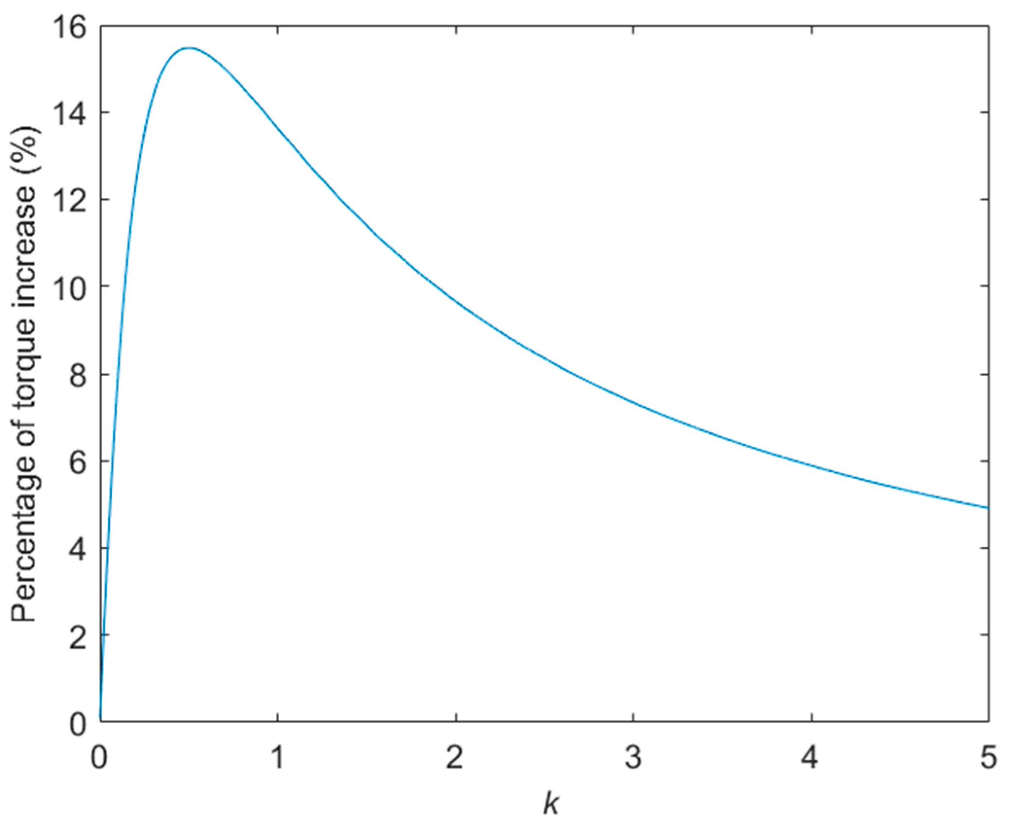
In order to highlight the impact on torque capacity, the percentage of “maximum torque” increase for SIAPMSMs as compared to classical PM machines ($\beta$ = 0) with the same set ($L_{dn},\rho$) and the same value of ($p{\Phi }_a{I}_m$) quantity is calculated as $\left(100\right({\Gamma }_{\mathrm{S}\mathrm{I}\mathrm{A}\mathrm{P}\mathrm{M}\mathrm{M}}-{\Gamma }_{\mathrm{P}\mathrm{M}})/{\Gamma }_{\mathrm{P}\mathrm{M}}$), where ${\Gamma }_{\mathrm{S}\mathrm{I}\mathrm{A}\mathrm{P}\mathrm{M}\mathrm{M}}$ and ${\Gamma }_{\mathrm{P}\mathrm{M}}$ are the SIAPMSM maximum torque and the PM motor maximum torque, respectively. The results are shown in Figure 10.

It is worth noting that, comparing to classical PM motors, the SIAPMSMs consistently permit higher torque. In addition, the maximum torque percentage increase is about 15.47% and is attained for particular ($L_{dn},\rho$) regions. Appendix A contains the analytical analysis of the percentage increase of the torque with some notes.

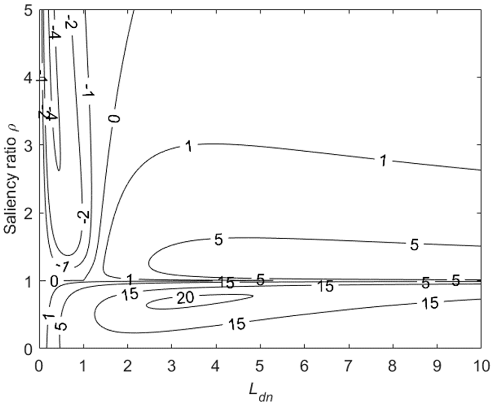
Figure 11 shows the power factor difference percentage between SIAPMSMs and classical PM synchronous motors in the ($L_{dn},\rho$) plane. The percentage increase is computed as $\left(100\right({PF}_{\mathrm{S}\mathrm{I}\mathrm{A}\mathrm{P}\mathrm{M}\mathrm{M}}-{PF}_{\mathrm{P}\mathrm{M}})/{PF}_{\mathrm{P}\mathrm{M}}$), where ${PF}_{\mathrm{S}\mathrm{I}\mathrm{A}\mathrm{P}\mathrm{M}\mathrm{M}}$ and ${PF}_{\mathrm{P}\mathrm{M}}$ are the SIAPMSM and PM motor power factors, respectively.

It should be highlighted that while the SIAPMSMs always help increase the torque compared to classical PM synchronous motors, this is not the case for the power factor. Indeed, as shown in Figure 11, for a significant area of the ($L_{dn},\rho$) plane, the SIAPMSMs will have a lower power factor compared to the classical PM synchronous motors. Nevertheless, the power factor drop is not large (≈$-4.2\%$ as a maximum).

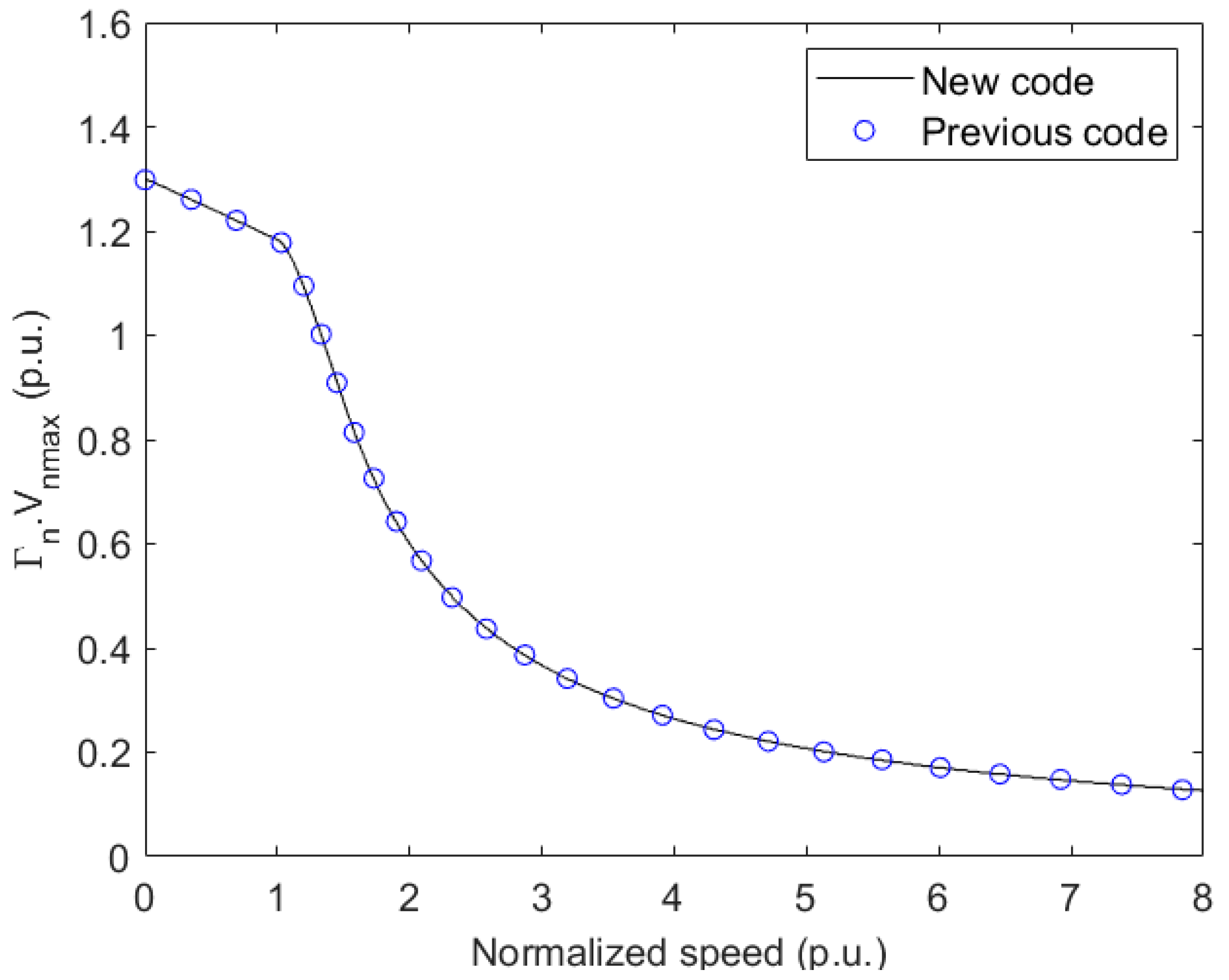
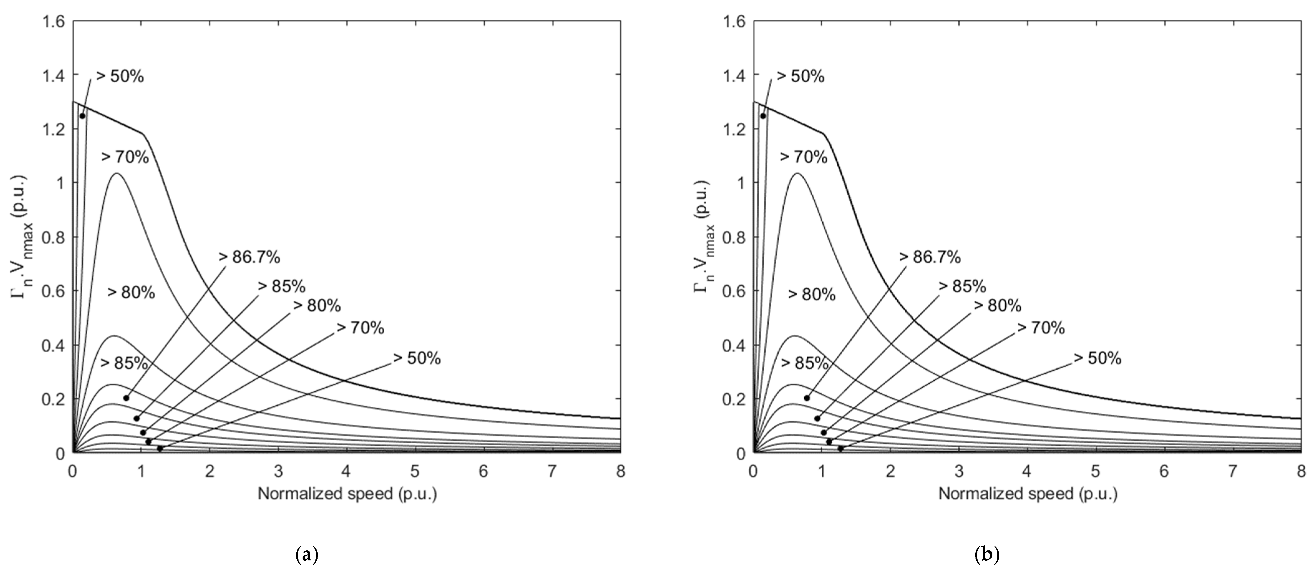
4.2.2. Validation of Developed Tool for the Case including the Electromagnetic Losses

Figure 12 compares maximum power capability curves for a SIAPMSM having $L_{dn}=2.5$, $\rho =0.6$, $R_{an}=0.1$, and $R_{fn}=20$ obtained using the new and old developed codes. Again, a good agreement is achieved.

Figure 13 compares, for the same machine, the efficiency maps drawn using the old and new code. As can be seen, the efficiency maps are also matching. As for the lossless case, the results from new and old codes have been also been compared for other values of $(L_{dn},\rho )$ couples; good agreements were always achieved.

As is the case with the old tools [9,13,14,15], this new tool can be used for the study of synchronous machines’ parameters’ effects on their performance. Since it is more general, more structures can be compared; this is very useful from an optimal design perspective.

5. Conclusions

This contribution presented a study that evaluated the effectiveness and accuracy of an algorithm used to compute the efficiency maps of Shifted Inductance Axes Permanent Magnet Synchronous Machines, taking into account electromagnetic losses. This tool can be used for both analysis and design purposes. The tool only considers simple electromagnetic loss models. However, it can be readily modified to incorporate more precise loss models and mechanical losses. From the obtained results, it can be concluded that the newly developed algorithm, while being assessed against previous ones, is more general and constitutes an interesting tool to conduct further interesting studies. The software codes, developed under the MATLAB environment, are made available for readers to test, evaluate, and perform their own proper studies.

Future works will focus on using a salient PM rotor instead of a non-salient one, studying classes of SIAPMSMs, and including the hybrid excitation.

References

- Gieras, J.F. Permanent Magnet Motor Technology: Design and Applications, 3rd ed.; CRC Press: Boca Raton, FL, USA, 2010. [Google Scholar]
- Boldea, I.; Tutelea, L.N.; Parsa, L.; Dorrell, D. Automotive electric propulsion systems with reduced or no permanent magnets: An overview. IEEE Trans. Ind. Electron. 2014, 61, 5696–5711. [Google Scholar] [CrossRef]
- Amara, Y.; Hlioui, S.; Ben Ahmed, H.; Gabsi, G. Power capability of hybrid excited synchronous motors in variable speed drives applications. IEEE Trans. Magn. 2019, 55, 1–12. [Google Scholar] [CrossRef]
- Zhao, W.; Lipo, T.A.; Kwon, B.-I. Optimal design of a novel asymmetrical rotor structure to obtain torque and efficiency improvement in surface inset PM motors. IEEE Trans. Magn. 2015, 51, 8100704. [Google Scholar]
- Zhao, W.; Chen, D.; Lipo, T.A.; Kwon, B.-I. Performance improvement of ferrite-assisted synchronous reluctance machines using asymmetrical rotor configurations. IEEE Trans. Magn. 2015, 51, 8108504. [Google Scholar] [CrossRef]
- Yang, H.; Li, Y.; Lin, H.; Zhu, Z.Q.; Lyu, S.; Wang, H.; Fang, S.; Huang, Y. Novel reluctance axis shifted machines with hybrid rotors. In Proceedings of the 2017 IEEE Energy Conversion Congress and Exposition (ECCE), Cincinnati, OH, USA, 1–5 October 2017. [Google Scholar]
- Takahashi, T.; Miyama, Y.; Nakano, M.; Yamane, K. Permanent Magnet Rotating Electric Machine. Japan PCT Patent Appl. WO 2019/064801 A1, 4 April 2019. [Google Scholar]
- Zhu, Z.Q.; Xiao, Y. Novel magnetic-field-shifting techniques in asymmetric rotor pole interior PM machines with enhanced torque density. IEEE Trans. Magn. 2022, 58, 8100610. [Google Scholar] [CrossRef]
- Diab, H.; Asfirane, S.; Amara, Y. Power Capability of Shifted Inductances Axes Permanent Magnet Machines. In Proceedings of the 2022 Joint MMM-Intermag Conference INTERMAG, New Orleans, LA, USA, 10–14 January 2022. [Google Scholar]
- Schiferl, R.F.; Lipo, T.A. Power capability of salient pole permanent magnet synchronous motors in variable speed drive applications. IEEE Trans. Ind. Appl. 1990, 26, 115–123. [Google Scholar] [CrossRef]
- Morimoto, S.; Takeda, Y.; Hirasa, T.; Taniguchi, K. Expansion of operating limits for permanent magnet motor by current vector control considering inverter capacity. IEEE Trans. Ind. Appl. 1990, 26, 866–871. [Google Scholar] [CrossRef]
- Soong, W.L.; Miller, T.J.E. Field-weakening performance of brushless synchronous AC motor drives. IEE Proc. Electr. Power Appl. 1994, 141, 331–340. [Google Scholar] [CrossRef]
- Amara, Y.; Hlioui, S.; Ben Ahmed, H.; Gabsi, M. Pre-optimization of hybridization ratio in hybrid excitation synchronous machines using electrical circuits modelling. Math. Comput. Simul. 2021, 184, 118–136. [Google Scholar] [CrossRef]
- Diab, H.; Asfirane, S.; Amara, Y.; Ben Ahmed, H.; Gabsi, M. Efficiency maps of synchronous machines based on electrical circuits modelling. In Proceedings of the Electrimacs 2022, Nancy, France, 16–19 May 2022. [Google Scholar]
- Amara, Y.; Ben Ahmed, H.; Gabsi, M. Hybrid Excited Synchronous Machines: Topologies, Design and Analysis; Wiley-ISTE: London, UK, 2023. [Google Scholar]
- Xie, Y.; Shao, J.; He, S.; Ye, B.; Yang, F.; Wang, L. Novel PM-Assisted Synchronous Reluctance Machines Using Asymmetrical Rotor Configuration. IEEE Access 2022, 10, 79564–79573. [Google Scholar] [CrossRef]
- Gosden, D.F.; Chalmers, B.J.; Musaba, L. Drive system design for an electric vehicle based on alternative motor types. In Proceedings of the 1994 Fifth International Conference on Power Electronics and Variable-Speed Drives, London, UK, 26–28 October 1994. [Google Scholar]
- Chalmers, B.J.; Akmese, R.; Musaba, L. PM reluctance motor with two-part rotor. In Proceedings of the IEE Colloquium on New Topologies for Permanent Magnet Machines (Digest No: 1997/090), London, UK, 18 June 1997. [Google Scholar]
- Chalmers, B.J.; Akmese, R.; Musaba, L. Design and field-weakening performance of permanent-magnet/reluctance motor with two-part rotor. IEE Proc. Electr. Power Appl. 1998, 145, 133–139. [Google Scholar] [CrossRef]
- Bianchi, N.; Bolognani, S.; Chalmers, B.J. Salient-rotor PM synchronous motors for an extended flux-weakening operation range. IEEE Trans. Ind. Appl. 2000, 36, 1118–1125. [Google Scholar] [CrossRef]
- Geng, W.; Zhang, Z.; Jiang, K.; Yan, Y. A new parallel hybrid excitation machine: Permanent-magnet/variable-reluctance machine with bidirectional field-regulating capability. IEEE Trans. Ind. Electron. 2015, 62, 1372–1381. [Google Scholar] [CrossRef]
- Wang, Y.; Deng, Z.; Wang, X. A Parallel hybrid excitation flux-switching generator DC power system based on direct torque linear control. IEEE Trans. Energy Convers. 2012, 27, 308–317. [Google Scholar] [CrossRef]
- Fernandez-Bernal, F.; Garcia-Cerrada, A.; Faure, R. Determination of parameters in interior permanent-magnet synchronous motors with iron losses without torque measurement. IEEE Trans. Ind. Appl. 2001, 37, 1265–1272. [Google Scholar] [CrossRef]
- Morimoto, S.; Tong, Y.; Takeda, Y.; Hirasa, T. Loss minimization control of permanent magnet synchronous motor drives. IEEE Trans. Ind. Electron. 1994, 41, 511–517. [Google Scholar] [CrossRef]
- Amara, Y.; Vido, L.; Gabsi, M.; Haong, E.; Ben Ahmed, A.H.; Lécrivain, M. Hybrid excitation synchronous machines: Energy-efficient solution for vehicles propulsion. IEEE Trans. Veh. Technol. 2009, 58, 2137–2149. [Google Scholar] [CrossRef]
- Soulard, J.; Multon, B. Maximum power limits of small single-phase permanent magnet drives. IEE Proc.-Electr. Power Appl. 1999, 146, 457–462. [Google Scholar] [CrossRef]
- New Generalized MATLAB Scripts Allowing for the Estimation of the Efficiency Maps for Synchronous Machines. Available online: https://1drv.ms/u/s!Ajoijjw3xSEGgQ5X5oEwhTCM9VXQ?e=zRUYP2 (accessed on 28 April 2023).
Figure 1.
SIAPMSM with two separate rotors (PM and variable reluctance rotors) [
6,
8].
Figure 2.
Improvement of torque density using SIAPMSM structures (current angle is the phase shift between phase armature currents and EMF). (a) Classical PM Machine, (b) SIAMPMSM .
Figure 3.
Examples of 2D SIAPMSM structures rotors [
4,
7,
8]. (
a) Asymmetrical rotor taken from [
4], (
b) Asymmetrical rotor taken from [
7], (
c) Asymmetrical rotor taken from [
Figure 4.
Park’s referential frames associated with the two rotors.
Figure 5.
Lossless SIAMPMSM equivalent circuits under motor mode operation in the () referential frame. (a) d axis equivalent circuit, (b) q axis equivalent circuit.
Figure 6.
SIAMPMM equivalent circuits including the electromagnetic losses. (a) d axis equivalent circuit, (b) q axis equivalent circuit.
Figure 7.
computation algorithm.
Figure 8.
Efficiency mapping computation algorithm.
Figure 9.
Comparison of maximum torque capabilities obtained using new and old codes .
Figure 10.
Torque increase in the () plane. (a) and (b) and
Figure 11.
Power factor difference in the () plane.
Figure 12.
Comparison of maximum torque capabilities obtained using new and old codes and
Figure 13.
Comparison of efficiency maps obtained using new and old codes , and . (a) Efficiency maps drawn using the old tool. (b) Efficiency maps drawn using the new tool.