Thermal Analysis of a Flux-Switching Permanent Magnet Machine for Hybrid Electric Vehicles

Abstract

This paper investigates the loss and thermal characteristics of a three-phase 10 kW flux-switching permanent magnet (FSPM) machine, which is used as an integrated starter generator (ISG) for hybrid electric vehicles (HEVs). In this paper, an improved method considering both DC-bias component and minor hysteresis loops in iron flux-density distribution is proposed to calculate core loss more precisely. Then, a lumped parameter thermal network (LPTN) model is constructed to predict transient thermal behavior of the FSPM machine, which takes into consideration various losses as heat sources determined from predictions and experiments. Meanwhile, a simplified one-dimensional (1D) steady heat conduction (1D-SHC) model with two heat sources in cylindrical coordinates is also proposed to predict the thermal behavior. To verify the two methods above, transient and steady thermal analyses of the FSPM machine were performed by computational fluid dynamics (CFD) based on the losses mentioned above. Finally, the predicted results from both LPTN and 1D-SHC were verified by the experiments on a prototyped FSPM machine.

1. Introduction

With the energy dilemma and environmental pollution becoming worse, electric-powered vehicles have attracted considerable attention due to their lower green gas emission and oil consumption [1]. Recent hybrid electric vehicles (HEVs) provide long-distance operation due to the optimal match between an engine powered by oil and electric motors powered by electricity stored in batteries. HEVs are widely researched by academics and have become dominant commercial products in EV markets [2,3]. For micro-hybrid EVs, an integrated starter generator (ISG) is the key component of both driving and generating systems, since it plays two major roles, namely, as a starter and a generator. Due to space and weight limitations, the rotor of an ISG is normally directly coupled to the flywheel of the engine in HEVs, where high torque (power) density, large overload torque capability, and high efficiency are expected. Hence, the flux-switching permanent magnet (FSPM) machine is considered as a promising candidate to be applied in electric vehicles, and aerospace and ship propulsion due to its high torque (power) density, high efficiency, and compact structure [4].

With the ever-increasing demand for power (torque) density, research on machine loss and temperature has become a hot topic. An accurate thermal model is an essential tool not only at the machine design stage but also for online prediction of temperature distribution [5]. While finite element method (FEM)-based and computational fluid dynamics (CFD)-based thermal models can achieve high accuracy, a lumped parameter thermal network (LPTN)-based model is often preferred thanks to its lower computational requirement and good accuracy [6,7,8].

In [9], the thermal influence of vehicle integration on the thermal load of an ISG was discussed by a FEM-based thermal model. In [10], an axially segmented FEM model of a FSPM machine was proposed to analyze the coupled electromagnetic–thermal performances. A thermal resistance network was established based on a nine-node model for an interior PM (IPM) machine and the transient temperature characteristics were obtained [11]. In [12], a numerical approach for estimation of convective heat transfer coefficient in the end region of an ISG was proposed, and both the local and averaged heat transfer coefficients were estimated. A systematic procedure to study the impact of each thermal phenomenon in IPM machines used for ISG was presented in [13]. In [14], a reduced model in a multi-physical electric machine optimization procedure was proposed.

The contribution of this paper is to propose two temperature prediction models for a 10 kW FSPM machine as an ISG for micro-hybrid vehicles; namely, a LPTN thermal model, and a one-dimensional (1D) steady heat conduction (SHC) (1D-SHC) model. The two methods can both quickly predict the internal temperature distribution of the FSPM machine. The results were verified by CFD and experiments to prove their accuracy.

Section 2 will propose an improved core loss model considering both the DC-bias component and minor hysteresis loops in iron flux-density, and the core loss of the FSPM machine is calculated and verified by experiments. Then, in Section 3 a LPTN model is proposed firstly to predict transient thermal behavior. After that, a simplified 1D-SHC thermal model is proposed to reveal the relationship between design parameters of a cooling jacket and thermal distribution of stator, and verified by experiments under different cooling conditions. In Section 4, both steady and transient thermal predictions are compared with those from ANSYS fluent-based CFD. Experiments with rising temperatures were conducted on a prototyped FSPM machine and are detailed in Section 5, followed by conclusions in Section 6.

2. Loss Prediction Model

The key dimensions of the studied FSPM machine are listed in

Table 1. Design specifications of the FSPM machine.

Parameter	Symbol	Value	Unit
DC-link voltage	UDC	144	V
Phase number	m	3	-
Stator slots	Ns	12	-
Rotor pole pairs	Nr	10	-
PM pole pairs	NPM	6	-
Rated power	PN	10	kW
Rated speed	nN	1000	r/min
Rated torque	TN	95.5	Nm
Stator outer diameter	Dso	260	mm
Rotor inner diameter	Dri	50	mm
Air-gap length	g0	0.9	mm
Stack length	La	55	mm

. In addition to electromagnetic parameters, the thermal conductivities, the specific heats, and densities of materials used for transient thermal analysis are presented in

Table 2. Thermal conductivities of materials.

Materials	Thermal Conductivity (W/m/°C)	Specific Heat Capacity (J/kg/°C)	Density (kg/m3)
Steel silicon	23	460	7650
Copper	380	385	8978
PM	9	504	7500
Aluminum	237	833	2688
Air	0.02624	1005	1.205

. The employed PM material was N35 and the silicon steel sheet was 35WW310.

The loss of the FSPM machine includes winding joule loss, core loss, eddy current loss in PMs, housing and frictional loss, and excess loss. According to the Bertotti G. model [15], the core loss of PM machines P_Fe consists of hysteresis loss, eddy current loss and excess loss, and the core loss yields:

$$P_{Fe}=P_h+P_c+P_e=k_{h}f{B}_m^{\alpha }+k_c{f}^{1.5}{B}_m^{1.5}+k_e{f}^2{B}_m^2$$

(1)

where Ph is hysteresis loss in W, Pc is the classical eddy current loss in W, P_e is the excess loss in W, k_h, k_c, and k_e are the corresponding coefficient of the above losses, respectively, f is the fundamental frequency of a magnetizing flux in Hz, and B_m is the maximum flux density in core in T.

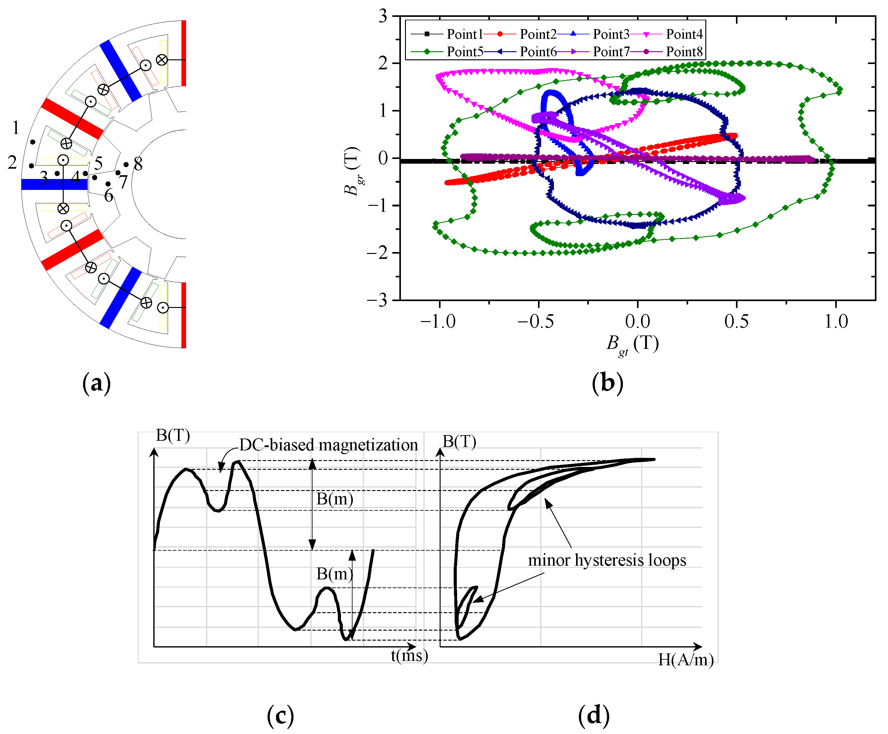
However, Equation (1) only works given a purely sinusoidal magnetizing flux. To exactly obtain the magnetizing flux-density characteristics in the FSPM machine core, eight key points located in stator and rotor respectively are selected, as shown in Figure 1a. Correspondingly, the resultant loci of the flux-density radial and tangential components (B_gr/B_gt) are predicted, as shown in Figure 1b. Clearly, for the stator points 1 and 2, the surrounded areas by the B_gr/B_gt loci are to be almost zero, which means the averaged B_gr/B_gt values are nearly zero. However, for points 3 and 4, the corresponding areas (the blue one and the pink one) are not centrosymmetric, which means a DC-biased component exists. For the points 5~8 in the rotor, the B_gr/B_gt loci are all centrosymmetric and the averaged values are close to zero. A typically DC-biased component and a minor hysteresis loop are shown in Figure 1c,d, respectively.

Unfortunately, the influence of magnetized DC-biased components and minor hysteresis loops are not well recognized in the commercial FEM software packages [16]. Hence, to predict the core loss of FSPM machines more precisely, an improved model considering both DC-biased component and minor hysteresis loops is proposed as follows. Assuming that the minor loop is similar to the major loop, the core loss can be divided into radial and tangential components. The total core loss, including the hysteresis loss [17], eddy current loss [18], and excess loss [19], can be obtained as follows:

$$P_h=k_{h}f{L}_a{\displaystyle \sum _{i=1}^{N_{elem}}\Delta A_i\left[\left({\displaystyle \sum _{j=1}^{N_{pr}^i}{B}_{rm}^{ij}{}^2}\right)\epsilon \left(\Delta B_r\right)+\left({\displaystyle \sum _{j=1}^{N_{pt}^i}{B}_{tm}^{ij}{}^2}\right)\epsilon \left(\Delta B_t\right)\right]}$$

(2)

$$P_c=\frac{K_c}{2{\pi }^2}\frac{L_a}{N_{setp}}\cdot {\displaystyle \sum _{k=1}^{N_{step}}{\displaystyle \sum _{i=1}^{N_{elem}}\Delta A_i\left[{\left(\frac{B_{rmi}^{k+1}-B_{rmi}^k}{\Delta t}\right)}^2+{\left(\frac{B_{tmi}^{k+1}-B_{tmi}^k}{\Delta t}\right)}^2\right]}}$$

(3)

$$P_e=\frac{K_e{L}_a}{N_{setp}}{\displaystyle \sum _{k=1}^{N_{step}}{\displaystyle \sum _{i=1}^{N_{elem}}\Delta A_i\left[{\left(\frac{B_{rmi}^{k+1}-B_{rmi}^k}{\Delta t}\right)}^{1.5}+{\left(\frac{B_{tmi}^{k+1}-B_{tmi}^k}{\Delta t}\right)}^{1.5}\right]}}$$

(4)

$$P_{Fe}=P_h+P_c+P_e$$

(5)

where N_elem is the finite elements number, ΔA_i is the ith finite element area in m², N_prⁱ and N_ptⁱ are the radial and tangential minor loops numbers of the ith element during one period, respectively, N_step is the calculation steps number, B_rm^ij and B_tm^ij are the maximum radial and tangential flux-densities of the jth hysteresis loop in the ith element in T, respectively, B_rmi^k and B_tmi^k are the maximum radial and tangential flux-density of the ith element in the kth calculation step in T, and Δt is the time step in s.

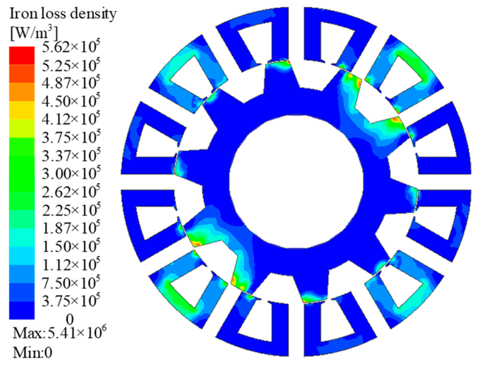
According to Equations (2)–(5), the core loss can be obtained by a combination platform of ANSYS and MATLAB, where based on ANSYS the detailed B_gr/B_gt results of each meshed iron element can be acquired, and based on MATLAB the core loss versus rotating speeds under different conditions can be assessed by a series of data processing calculations according to Equations (2)–(5). 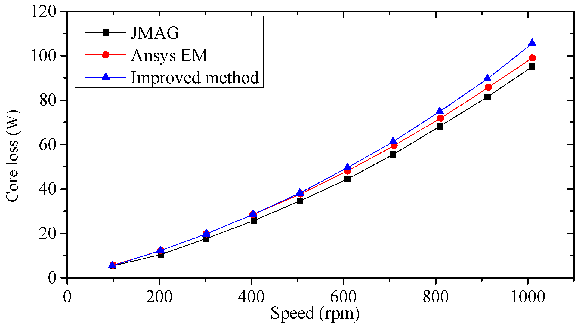The no-load core loss density distribution of the stator and rotor is shown in Figure 2. Consequently, the predicted core losses versus rotor speed are compared with those obtained by commercial software, e.g., by JMAG and ANSYS EM as shown in Figure 3. It can be seen that the core losses obtained by the improved method are slightly higher than those from software, which validates the influence of the DC-biased component and minor hysteresis loop, and also validates the feasibility of the improved core loss prediction method.

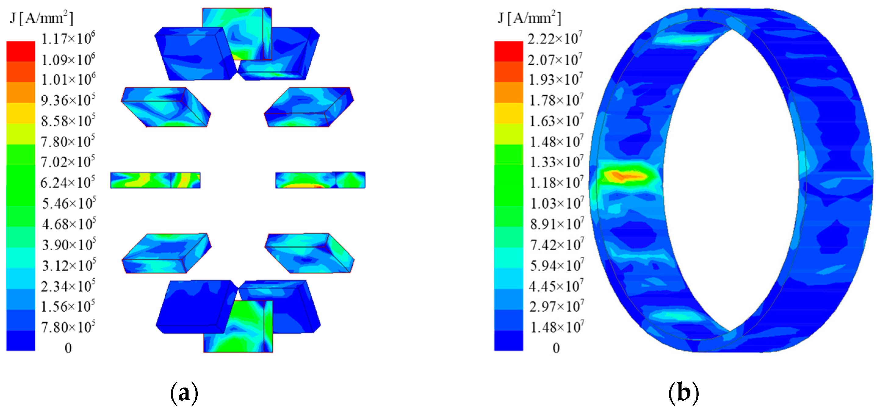
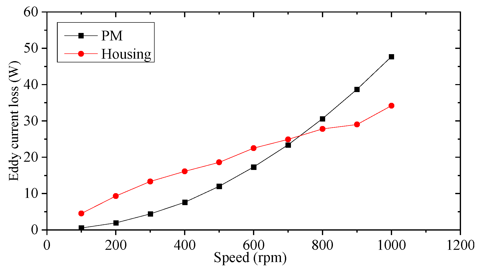
In addition, the no-load eddy current density distribution derived by 3D-FEM is shown in Figure 4. The resulting no-load eddy loss in PMs P_pmc and housing P_hc versus rotating speeds are shown in Figure 5. It can be found that with the increase of the speed, the eddy current losses in PMs and housing increase gradually, which is caused by the air-gap harmonic fields and can be calculated by Equation (6) [20],

$$P_{eddy}=\frac{1}{T}{\displaystyle \underset{t_c}{\int }{\displaystyle \sum _{i=1}^k{J}_e^2{\Delta }_{Ai}{\sigma }_r^{-1}{L}_{a}dt}}$$

(6)

where P_eddy is the eddy current loss in PM and housing in W, J_e is the current density in each element in A/m², Δ_Ai is the ith element area in m², σ_r is the conductivity of the eddy current zone in S/m, and t_c is the time corresponding to a period in each element in s.

The frictional loss P_fri of the FSPM machine yields [21]:

$$P_{fri}=16N_r{\left(\frac{v_r}{40}\right)}^3\sqrt{\frac{L_a}{19}\times {10}^3}$$

(7)

where v_r is the rotor peripheral speed in m/s. It is found that P_fri = 10.7 W under the rated speed of 1000 r/min.

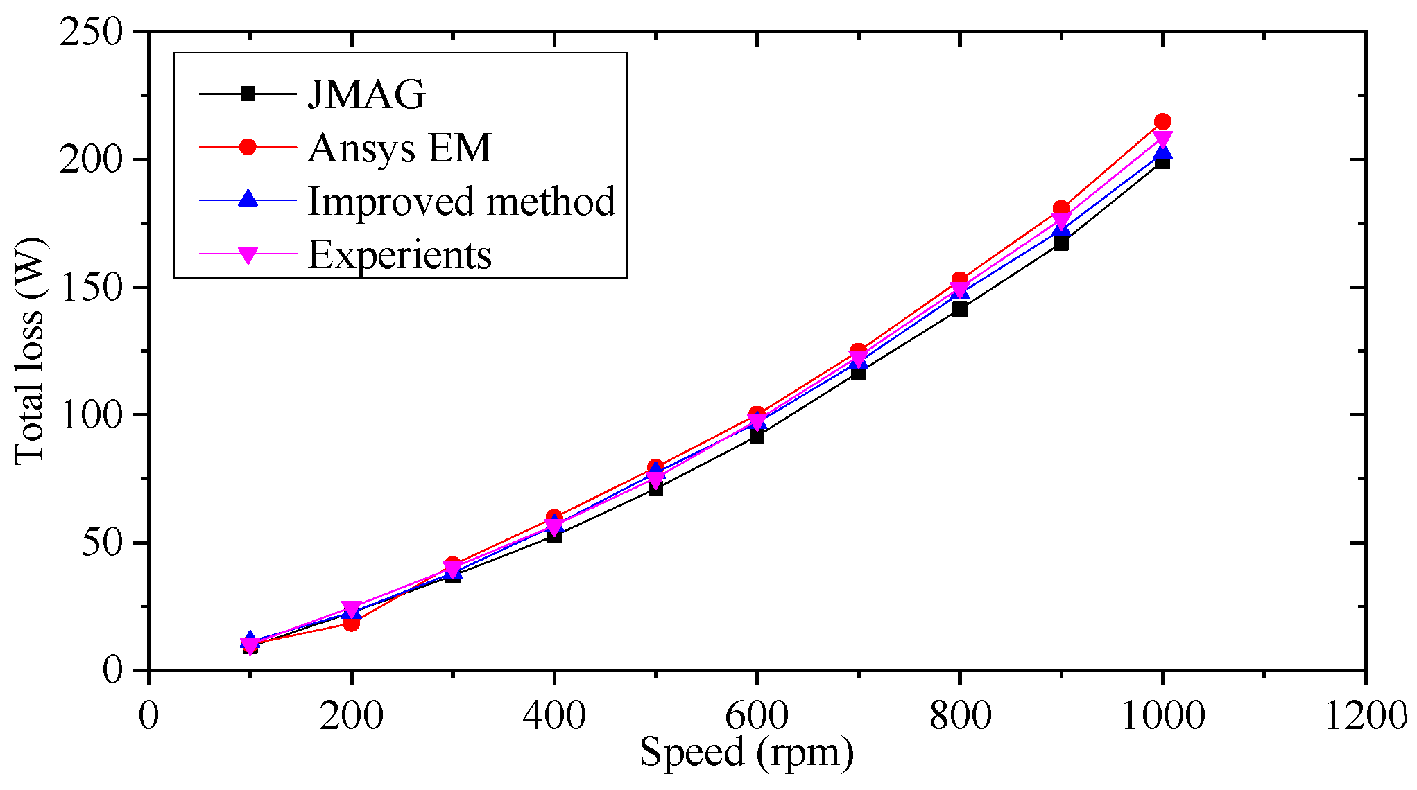
Finally, a no-load test under different rotation speeds is conducted on a prototyped FSPM machine to verify the predicted results, where the machine is controlled by a DSP-based controller and the input power is obtained by a power analyzer. The frictional loss is so small that it can be neglected. Therefore, the input power is equal to the total loss. The total losses versus rotor speeds by different methods are compared in Figure 6. Compared with the results obtained by commercial software, the predicted core losses derived by the improved method agree with the measurements with the smallest deviations.

3. Two Thermal Models

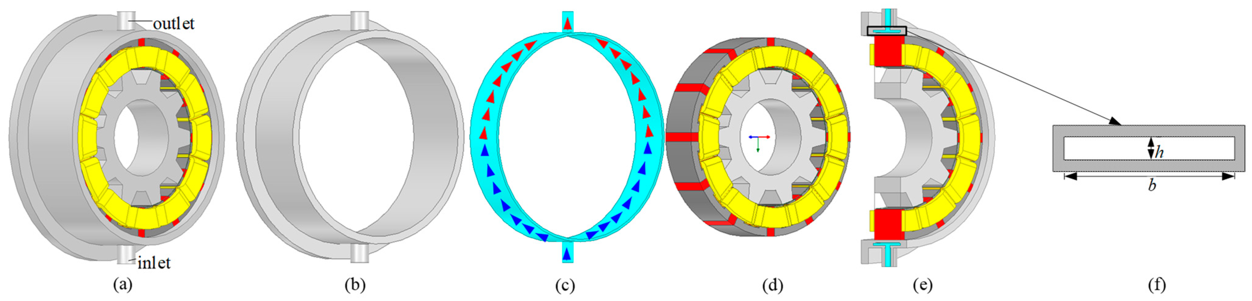
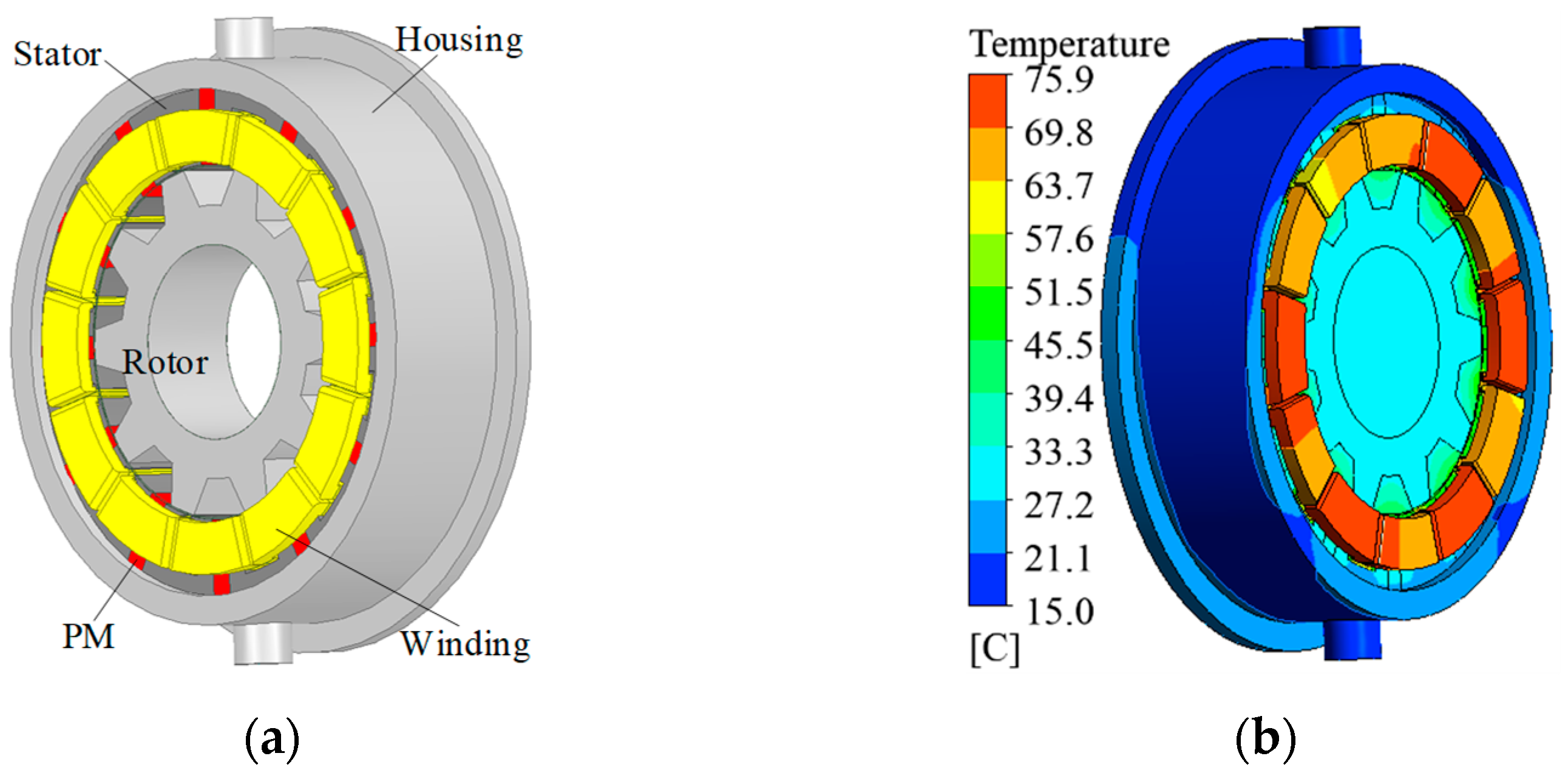
For the prototyped FSPM machine, a circumferential water jacket with one cooling duct is introduced in the stator housing as shown in Figure 7. The coolant channel of the casing adopts a single-layer water jacket cooling structure. Figure 7a shows the schematic diagram of the FSPM machine structure. Figure 7b–d show the housing, coolant flow path, and machine assembly, respectively. Figure 7b shows the cross-sectional diagram of the machine, and Figure 7c shows the cross-sectional diagram of the cooling duct. Arrows are used in Figure 7c to indicate the flow path of the coolant. The blue arrow represents the low temperature coolant near the inlet, while the red arrow represents the coolant that has been heated through heat exchange. The fluid running inside the cooling duct can be modeled as the movement of fluid in a rectangular channel using dimensionless numbers. Consequently, the convection coefficient can be obtained in the following stages.

Firstly, with the cooling jacket cross-section in Figure 7c, the Prandtl number of the fluid P_rf yields

$$P_{rf}=\frac{c_f{\eta }_f}{{\lambda }_f}$$

(8)

where c_f is the specific heat capacity of fluid in J/(kg·°C), η_f is fluid dynamic viscosity in N·s/m², and λ_f is the fluid thermal conductivity in W/(m·°C).

Secondly, the Reynolds number of fluid R_e yields

$$R_e=\frac{\upsilon d_e}{v_f}$$

(9)

where υ is the velocity of fluid in m/s, v_f is the fluid kinetic viscosity in m²/s, and d_e is the hydraulic radius in m by Equation (10).

$$d_e=\frac{4A_{cs}}{s}=\frac{4bh}{2\left(b+h\right)}$$

(10)

where A_cs is a cross-section area of a single cooling duct in m². s, b, and h are the wetted perimeter, width, and height of cooling duct in m, respectively.

Approximately, in a circumferential cooling duct, the velocity of fluid can be figured out as

$$\upsilon =\frac{Q}{A_{cs}}$$

(11)

where Q is the fluid quantity in kg/s.

According to the value of Re, the fluid flow can be divided into turbulence flow and laminar flow. The Nusselt number of the laminar flow N_ufl yields [22],

$$N{u}_{f\mathrm{l}}=0.644(R{e}^{0.5})P_r{{}_f}^{\frac{1}{3}}$$

(12)

For turbulence flow, the Nusselt number N_uft yields

$$N{u}_{ft}=0.023\left({Re}^{0.8}\right)P_{rf}{}^{0.4}{\left(\frac{{\eta }_f}{{\eta }_w}\right)}^{0.14}$$

(13)

where η_w is the dynamic viscosity of housing in N·s/m².

Based on the similarity criterion of fluid [22], the convection heat transfer coefficient h_f0 yields

$$h_{f0}=\frac{N{u}_f{\lambda }_f}{d_e}$$

(14)

Considering that turbulence flow shows a better heat dissipation than laminar flow, the former is employed in the cooling jacket, where the convection heat transfer coefficient h_f of the cooling jacket is affected by the geometric parameters and the velocity of the fluid, and can be given by

$$h_f={\lambda }_f\frac{b+h}{2bh}{\left(\frac{2Q}{v_f\left(b+h\right)}\right)}^{0.8}{P}_r{}_f^{0.4}{\left(\frac{{\eta }_f}{{\eta }_w}\right)}^{0.14}$$

(15)

From Equation (15), when the fluid quantity keeps constant, as the cross-sectional area of the cooling ducts decreases, the convection coefficient of the cooling jacket increases. However, a small cross-section cooling duct is not only difficult to manufacture, but also may lead to high inlet velocity and high hydraulic pressure, which causes the corrosion of cooling duct and deteriorates the operation stability. In the following, two thermal models are proposed, one a LPTN model and the other a 1D-SHC model.

3.1. Lumped Parameter Thermal Network Model

A LPTN model enables the heat flow and the temperature distribution inside the machine by means of an equivalent thermal circuit, which is composed of heat sources, thermal resistances, and thermal capacitances. For the convenience of calculation and improved accuracy, three assumptions are made as follows [23,24,25]:

• Symmetrical temperature distribution and the same cooling conditions along the circumference;
• Uniformly distributed thermal capacity and heat generation;
• Independent heat flow in radial and axial directions

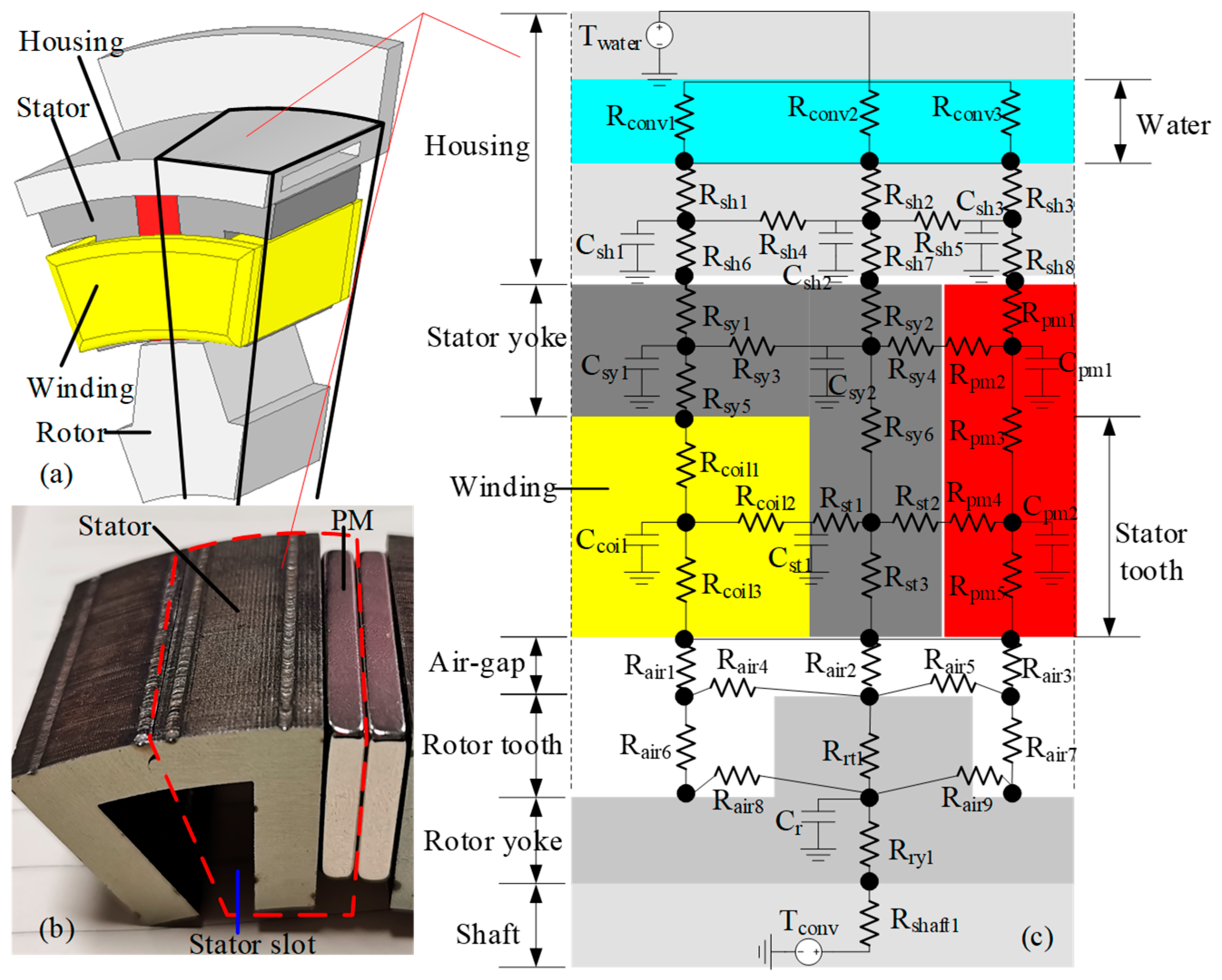
To simplify the calculation load, only 1/24 of the FSPM machine is modeled as shown in Figure 8 due to symmetry, where the heat sources including stator/rotor core losses, PM/housing eddy current losses, and windings joule loss are considered. The thermal resistances and capacitances can be determined according to the machine geometry and the physical properties of materials.

Table 3. Component thermal resistances of the LPTN model.

Thermal Resistances	Value (°C/W)	Thermal Resistances	Value (°C/W)
Rsh1, Rsh2, Rsh3	0.0004307	Rst1, Rst2	0.1479
Rsh4	0.1094	Rst3	0.01449
Rsh5	0.07664	Rcoil1	0.6297
Rsh6, Rsh7, Rsh8	0.0004469	Rcoil2	4.895
Rsy1, Rsy2	0.00359	Rcoil3	0.7244
Rsy3	0.2107	Rpm1	0.01197
Rsy4	0.1128	Rpm2	0.04699
Rsy5	0.003729	Rpm3	0.05441
Rsy6	0.01632	Rpm4	0.2054
Rair1, Rair2, Rair3	1.096	Rpm5	0.04829
Rair4, Rair5	596	Rrt1	0.02435
Rair6, Rair7	27.84	Rry1	0.03246
Rair8	30.76	Rshaft1	0.2613
Rair9	56.14	-	-

and

Table 4. Thermal capacitances of the LPTN model.

Thermal Capacitance	Value (J/°C)	Thermal Capacitance	Value (J/°C)
Csh1	30.82	Cst1	71.37
Csh2	21.86	Ccoil1	0.0036
Csh3	10.75	Cpm1	10.67
Csy1	31.63	Cpm2	33.14
Csy2	22.98	Cr	497.2

list the corresponding resistances and capacitances of the LPTN model. A preliminary selection of the resistances and capacitances can be determined according to the machine geometry and physical properties of the materials used [26].

With the convection heat transfer coefficient, the thermal resistance R_convi (i = 1, 2, 3) representing the heat dissipation by cooling medium convection between the housing external surface and ambient can be calculated by Equation (16) [25],

$$R_{convi}=\frac{1}{h_{convi}{A}_{convi}}$$

(16)

where R_convi is the thermal resistance due to convection heat transfer in °C/W, h_convi is the convection heat transfer coefficient in W/(m²·°C), and A_convi is the convective area in m². Here, the area of the end-part winding is considered.

Since the heat exchange between stator and rotor through the air-gap is assumed to be only by convection, Equation (16) is also used for the calculation of the thermal resistances R_airi.

In addition to heat convection, heat conduction is also an important way for heat dissipation. The resistance representing the heat flow in the radial direction is modeled by using Equation (17),

$$R_{radial}=\frac{ln\left(r_o/r_i\right)}{2\pi \lambda L}$$

(17)

where r_o and r_i are the outer and inner diameter of the cylinder in m, λ is the thermal conductivity of the material in W/m/°C, and L is the cylinder length in m.

In the tangential direction, the thermal resistance due to conduction heat transfer is given by,

$$R_{tangential}=\frac{l}{\lambda A_{cond}}$$

(18)

where l is a portion length of the path considered in m, and A_cond is the area for the conduction in m².

Figure 8a,b show the 3D module structure and modular stator element of the FSPM machine. Based on the thermal resistances above, a thermal resistance network of the 1/24 machine is constructed as shown in Figure 8c, where R_sh1-R_sh8, R_sy1-R_sy6, R_air1-R_air9, R_st1-R_st3, R_coil1-R_coil3, and R_pm1-R_pm5 represent the thermal resistances of the housing, stator yoke, air-gap, stator tooth, stator winding coils, and PMs. R_rt1, R_ry1, and R_shaft1 represent the thermal resistances of rotor tooth, rotor yoke, and shaft, respectively. C_sh1-C_sh3, C_sy1-C_sy2, C_st1, C_coil1, C_pm1-C_pm2, and C_rt represent the thermal capacitances of the housing, stator yoke, stator tooth, winding coils, PMs, and rotor tooth. Here, since the heat dissipated by forced convection is much larger than that by radiation, the radiation heat dissipation is ignored.

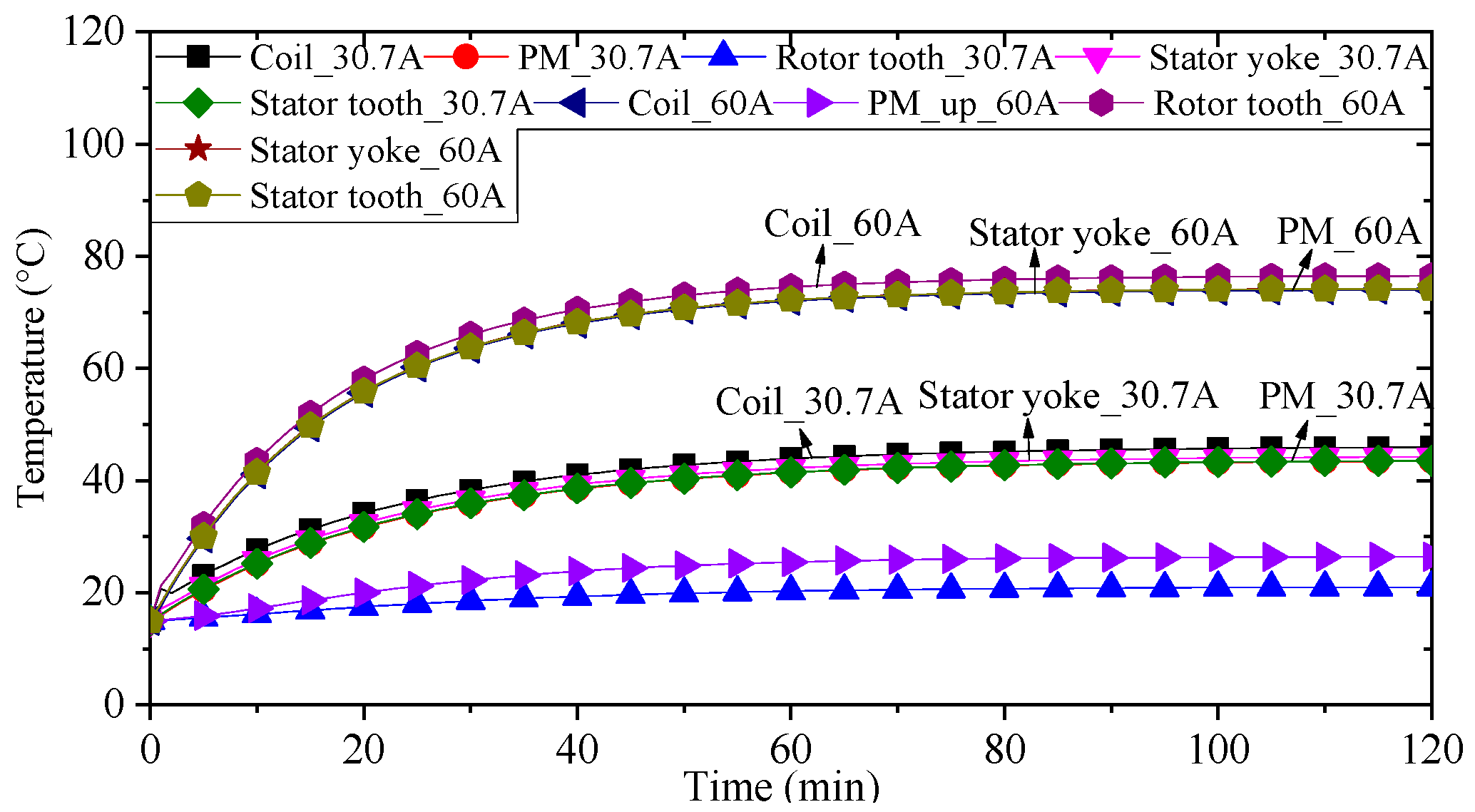
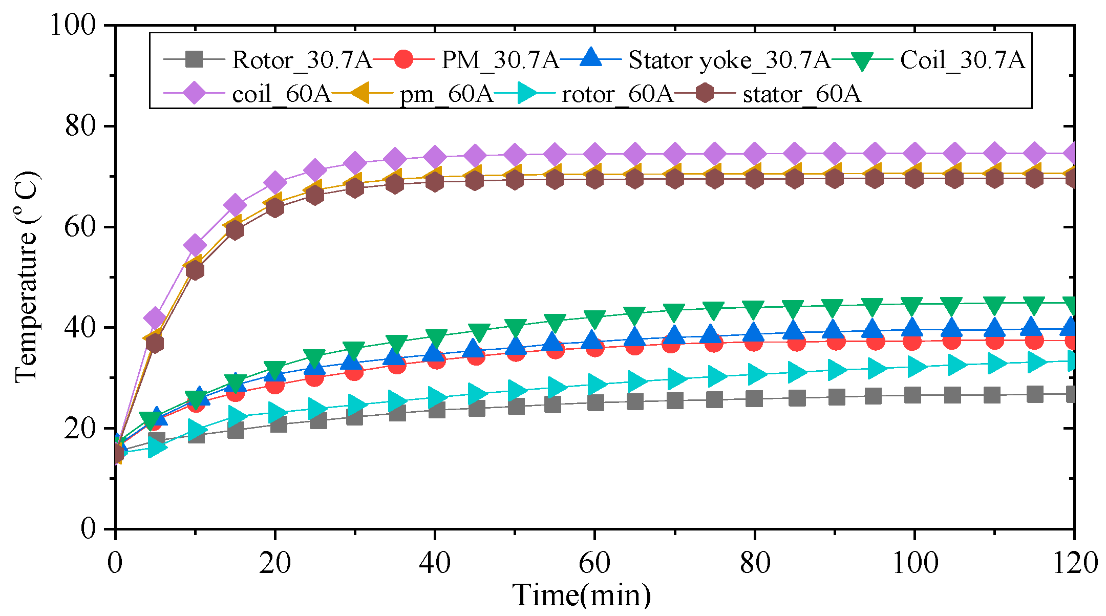
Under two typical operation conditions, i.e., the speed of 1000 r/min and the phase current of 30.7 A (RMS) and 60 A (RMS), the transient temperature rises of different components under forced water cooling are obtained by the LPTN model, and the results are shown in Figure 9. It takes around 70 min for the machine under water cooling to reach a thermal steady state where the armature windings have the highest temperatures (45.7 °C@30.7 A and 82.8 °C@60 A under water cooling). In addition, since the PMs are mounted on the stator, the temperature of the PMs is very close to that of the stator core, exhibiting the advantage of FSPM machines.

3.2. One-Dimensional Steady Heat Conduction Model

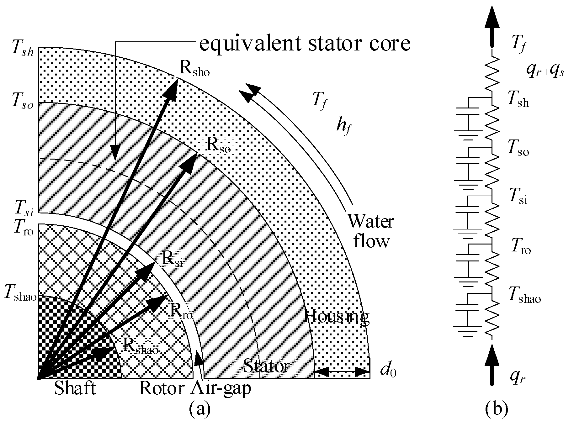
Generally, LPTN and FEM have been widely employed in thermal analysis of electrical machines. However, these two methods are normally time-consuming and require complicated modeling. For water-cooling machines, in order to select a reasonable flow rate of coolant, a 1D-SHC approach is proposed based on heat transfer and fluid mechanics as shown in Figure 10, and the relationship between the internal temperature of the stator and the coolant flow rate and coolant temperature is obtained.

It should be noted that the 1D-SHC model is based on the following assumptions. (1) The loss is uniformly distributed in each component of the machine. (2) The heat generated by joule loss and stator core loss is only dissipated by the housing. (3) The stator laminations, windings, and PMs are simplified to a homogeneous heating unit and the equivalent averaged thermal conductivity λ_avg yields [26,27]:

$${\lambda }_{ave}=\frac{A_s+A_{wind}+A_{pm}}{\frac{A_s}{{\lambda }_s}+\frac{A_{wind}}{{\lambda }_{cu}}+\frac{A_{pm}}{{\lambda }_{pm}}}$$

(19)

where A_s, A_wind, and A_pm are the cross-section area of the stator, windings, and PMs in m², respectively, λ_s, λ_wind, and λ_pm are the thermal conductivity of stator, windings, and PMs in W/(m·°C).

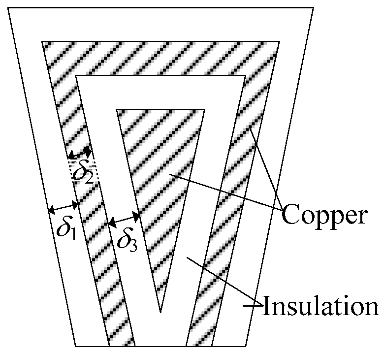
The winding and insulation layering is used to calculate the thermal conductivity of the stator windings. Figure 11 shows the equivalent diagram of the winding structure, where the insulation and windings are arranged with intervals. The slot filling factor is set as 0.35 according to the prototyped machine. The equivalent winding thermal conductivity yields:

$${\lambda }_{wind}={\displaystyle \sum _{\mathrm{i}=1}^n{\delta }_i/{\displaystyle \sum _{i=1}^n\frac{{\delta }_i}{{\lambda }_i}}}$$

(20)

where δ_I is the thickness of the ith layer in m, λ_i is the thermal conductivity of the ith layer in W/(m·°C).

Then, the equivalent volumetric heat generation of stator q_Vs and rotor q_Vr can be obtained by

$$\{\begin{array}{l}{P}_{eave}=\frac{P_s{V}_s+P_{cu}{V}_{cu}+P_{pm}{V}_{pm}}{V_s+V_{cu}+V_{pm}}\\ q_{Vs}=\frac{P_{eave}}{V_{equ}} \\ q_{Vr}=\frac{P_r}{V_r} \end{array}$$

(21)

where P_eave is equivalent average loss in W, P_s, P_cu, P_pm, and P_r are the stator core loss, winding joule loss, eddy current loss in PMs, and rotor core loss in W, respectively, V_s, V_cu, V_pm, V_equ, and V_r are the volume of stator, winding, PM, equivalent stator, and rotor in m³, respectively.

Since the thermal model is simplified into a 1D-SHC model, the heat flux density of stator/rotor (q_s/q_r) yields

$$\{\begin{array}{c}{q}_s=q_{Vs}/S_s\\ q_r=q_{Vr}/S_r\end{array}$$

(22)

where S_s/S_r is the cross-section area of stator/rotor lamination in m².

The inlet and outlet temperature of the cooling fluid can be detected by a hand-held infrared thermometer. Thus, the temperature of the fluid T_f equals

$$T_f=\frac{T_i+T_o}{2}$$

(23)

where Ti/To is the inlet/outlet temperature of the fluid in °C.

According to the 1D thermal circuit in Figure 10b, the temperature of housing T_sh can be derived by

$$T_{sh}=T_f+\frac{q_r}{\pi h_f\left(R_{sho}-R_{shao}\right)}+\frac{q_s}{\pi h_f\left(R_{sho}-R_{si}\right)}$$

(24)

where hf is the fluid convection coefficient in W/(m²·K), Rsho is the housing outer radius in m, Rshao is the shaft outer radius in m, and Rsi is the stator inner radius in m.

The temperature of stator yoke T_sy yields

$$T_{sy}=T_{sh}+\left(q_r+q_s\right)\frac{ln\left(R_{sho}/R_{so}\right)}{2\pi h_{sh}}$$

(25)

where R_so is the stator outer radius in m, and h_sh is the housing thermal conductivity in W/(m·°C).

The differential equations of the heat conduction and the boundary conditions for a cylinder with uniform heat generation are as follows [23]:

$$\{\begin{array}{c}\frac{1}{r}\cdot \frac{d}{dr}\left(r\cdot \frac{dt}{dr}\right)+\frac{q_r}{{\lambda }_r}+\frac{q_r+q_s}{{\lambda }_{avg}}=0\\ T=T_{sy},r=R_{so};\frac{dt}{dr}=0,r=0\end{array}$$

(26)

where λ_r is the rotor thermal conductivity in W/(m·°C).

The thermal distribution of the machine can be given by

$$\{\begin{array}{c}{h}_f={\lambda }_f\frac{b+h}{2bh}{\left(\frac{2v}{v_f}\right)}^{0.8}{Pr}_f^{0.4}{\left(\frac{{\eta }_f}{{\eta }_w}\right)}^{0.14}\\ T\left(r\right)=\frac{R_{so}{}^2}{4}\left(\frac{q_r}{{\lambda }_r}+\frac{q_r+q_s}{{\lambda }_{avg}}\right)\end{array}$$

(27)

Hence, the stator teeth temperature can be obtained by

$$\begin{array}{l}{T}_{st}=\frac{T_i+T_o}{2}+\left(q_r+q_s\right)\left(\frac{ln\left(R_{sho}/R_{so}\right)}{2\pi h_{sh}}+\frac{R_{so}{}^2-R_{si}{}^2}{4{\lambda }_{avg}}\right)+\\ \hspace{1em}\hspace{1em}\frac{1}{\pi h_f}\left(\frac{q_r}{R_{sho}-R_{shao}}+\frac{q_s}{R_{sho}-R_{si}}\right)+\frac{\left(R_{so}{}^2-R_{si}{}^2\right)q_r}{4{\lambda }_r}\end{array}$$

(28)

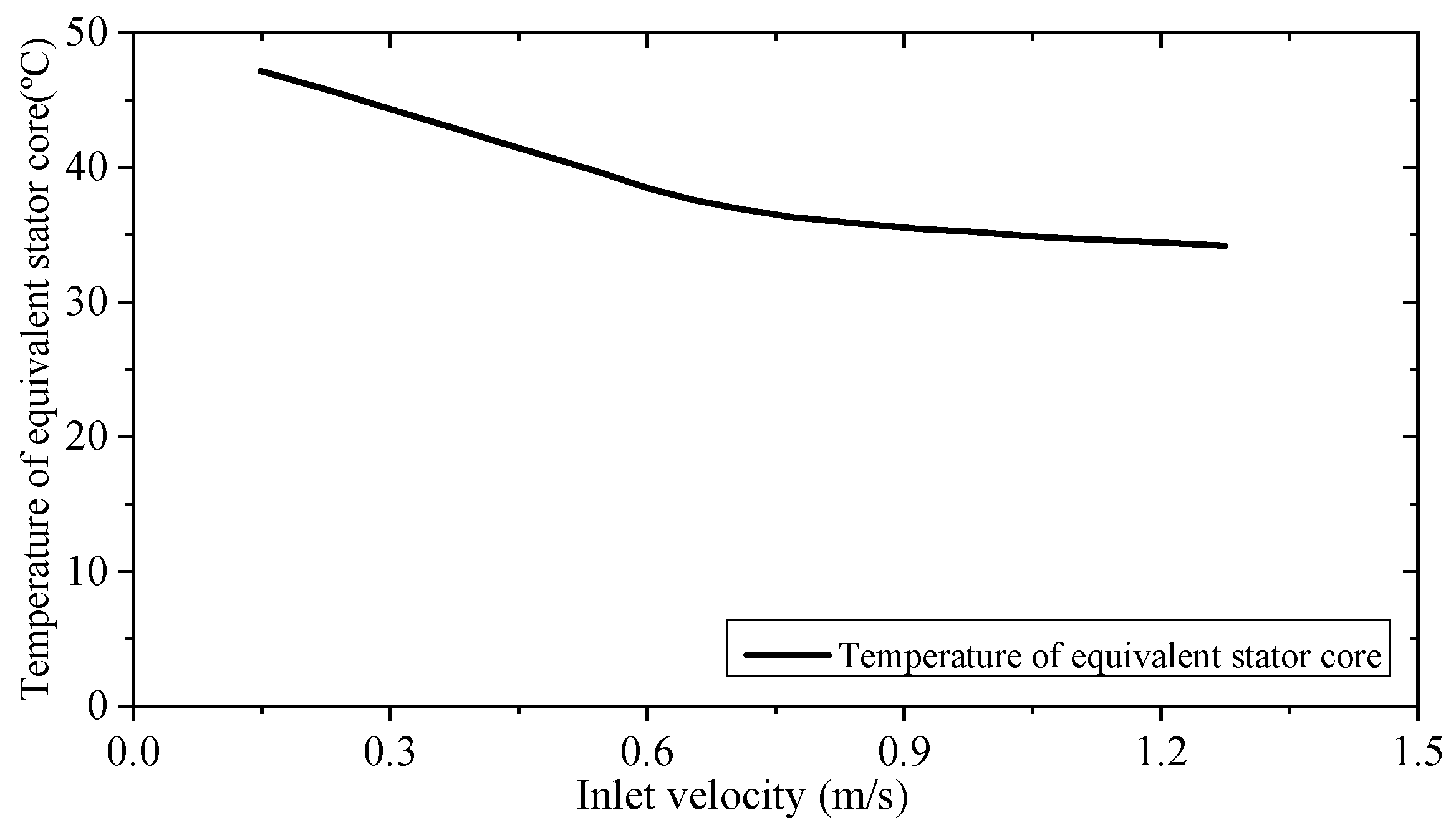
According to Equations (11), (15) and (28), as the average velocity of fluid increases, the convection coefficient of the cooling jacket increases and the stator temperature decreases. According to the prototype dimensions, when the no-load machine is running at the speed of 1000 r/min, the relationship between the temperature of the equivalent stator core (marked in Figure 10) and the inlet velocity can be obtained as shown in Figure 12. Obviously, as the inlet velocity of water increases to 0.6 m/s, the equivalent stator core temperature decreases almost linearly. When the inlet velocity increases to 1 m/s, the stator core temperature varies nonlinearly and slowly, so 1 m/s is set as the rated cooling inlet velocity of the FSPM machine, corresponding to a pump flow of 1800 L/h.

4. CFD-Based 3D Temperature Field Verification

In order to verify the proposed LPTN and 1D-SHC models, based on the loss calculated by FEM, a 3D-CFD thermal model is built as shown in Figure 13a. Figure 13b corresponds to water cooling.

When the cooling jacket is injected with an total inlet flow of 1800 L/h, a phase current of 30.7 A and 60 A, as well as a speed of 1000 r/min, the transient temperature rises of different components under forced water cooling are obtained as shown in Figure 14. It can be seen that the armature windings achieve the highest temperature under forced water-cooling conditions, whereas the armature windings temperature difference is 31 °C when the armature current is 30.7 A and 60 A, respectively. In addition, compared with the results obtained by the LPTN model shown in Figure 9, both the steady-state and transient results agree well.

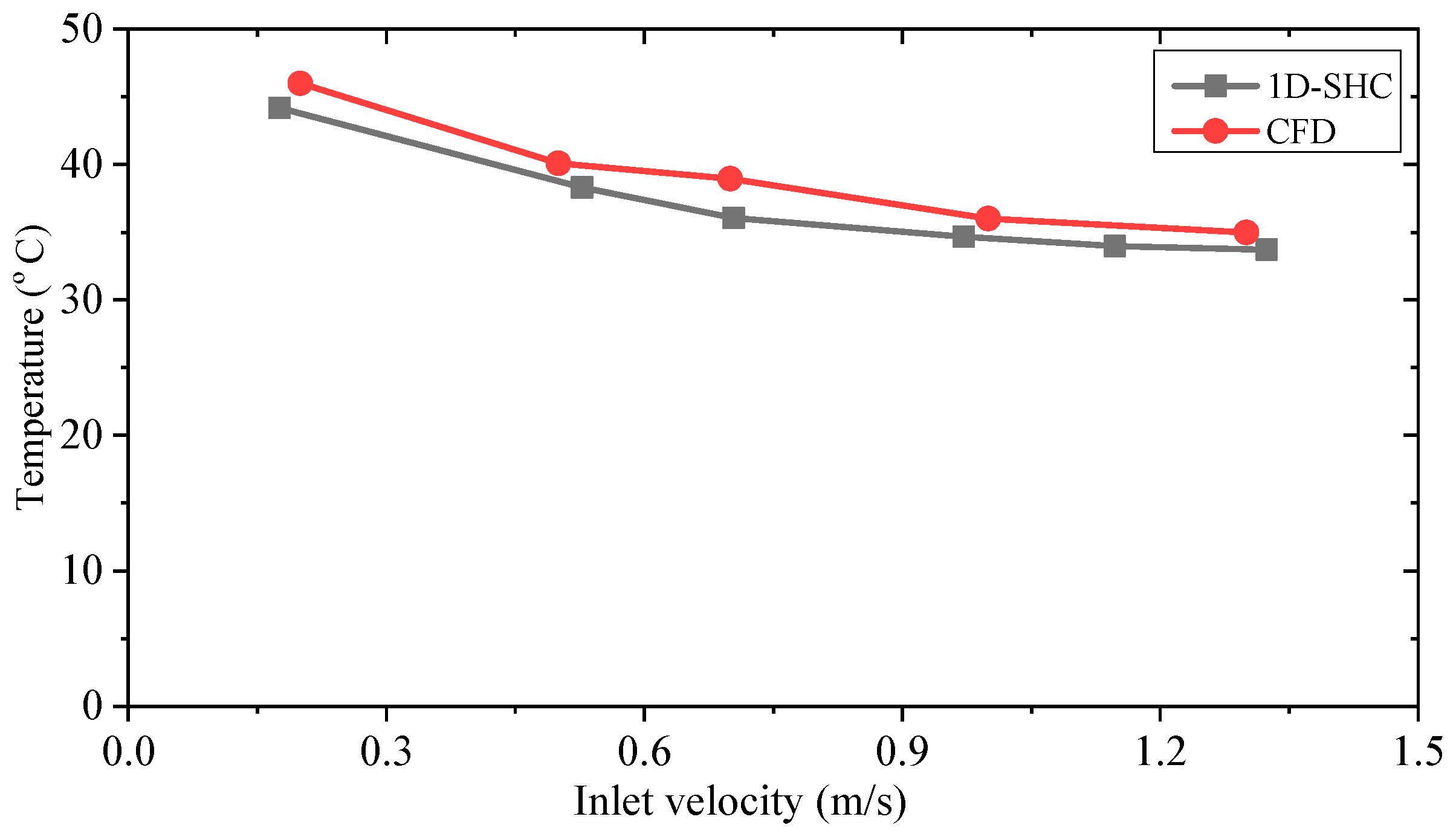
On the other hand, to verify the 1D-SHC model, the predicted equivalent stator core temperatures vs. inlet velocity by 1D-SHC and CFD are compared in Figure 15, where the operation status and cooling conditions are consistent with the 1D-SHC model. In addition to predicted temperatures, the time consumed by the three methods is compared in

Table 5. Comparison of time consumed by temperature prediction methods.

Temperature Prediction Methods	Steady State	Transient
LPTN method	2 s	7 s
1D-SHC method	0.6 s	1.4 s
CFD method	11 min	100 min

. Obviously, both the LTPN and 1D-SHC methods can save considerable time, which is favorable for the optimal design of machines.

5. Experiment Verification

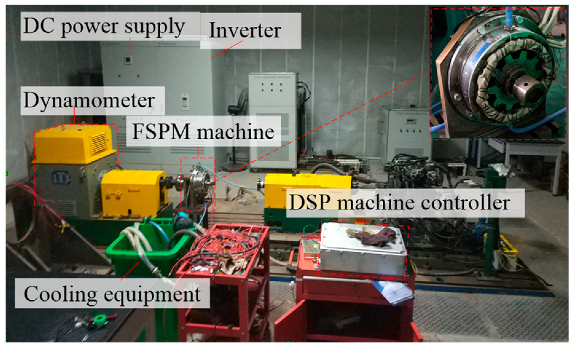
To validate the proposed thermal prediction models, a prototyped FSPM machine was manufactured and tested as shown in Figure 16. The prototyped FSPM machine was driven by an inverter supplied by a DC power source and the output shaft was directly connected with a dynamometer machine, in which a torque transducer and a resolver were equipped to measure torque and (rotor position) speed, respectively. 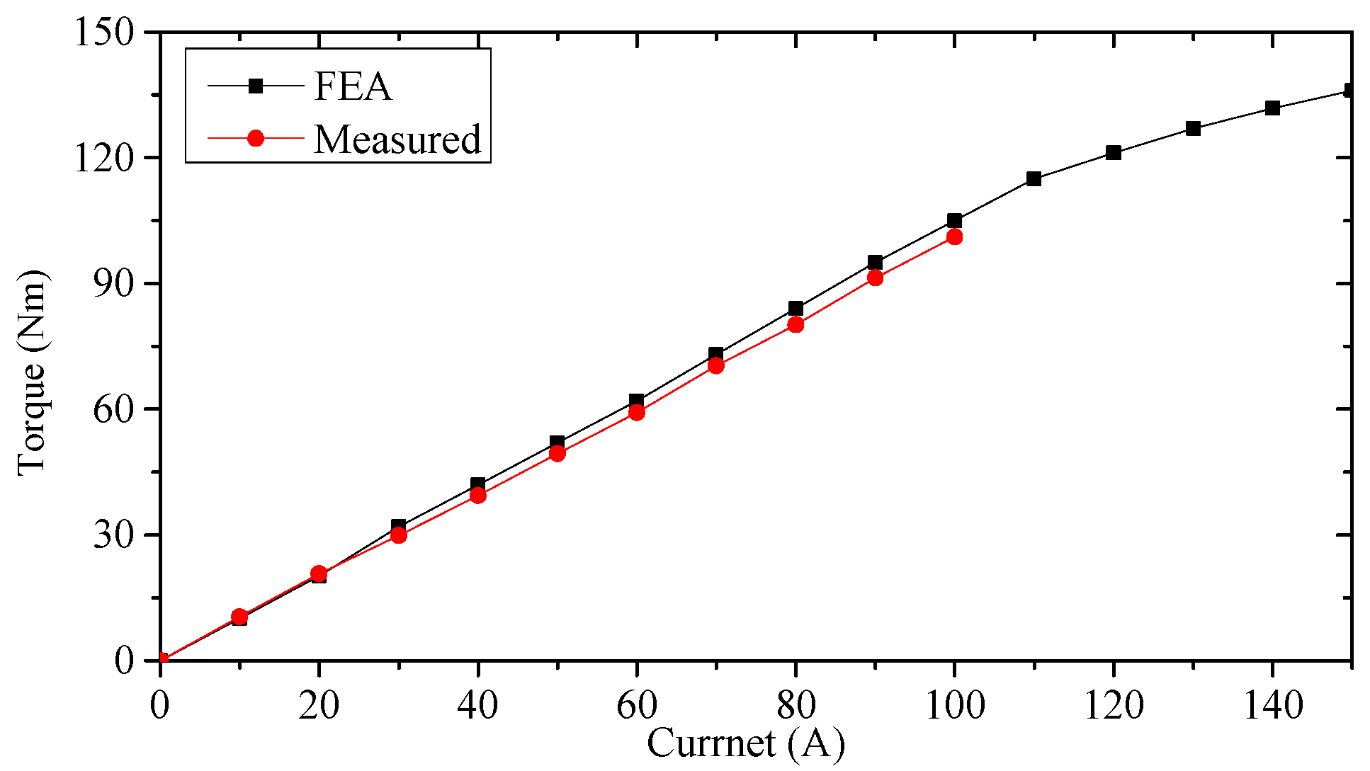Figure 17 compares the FEA-predicted and experimental results of torque versus phase currents. It can be seen that good agreements can be achieved with a deviation below 8%.

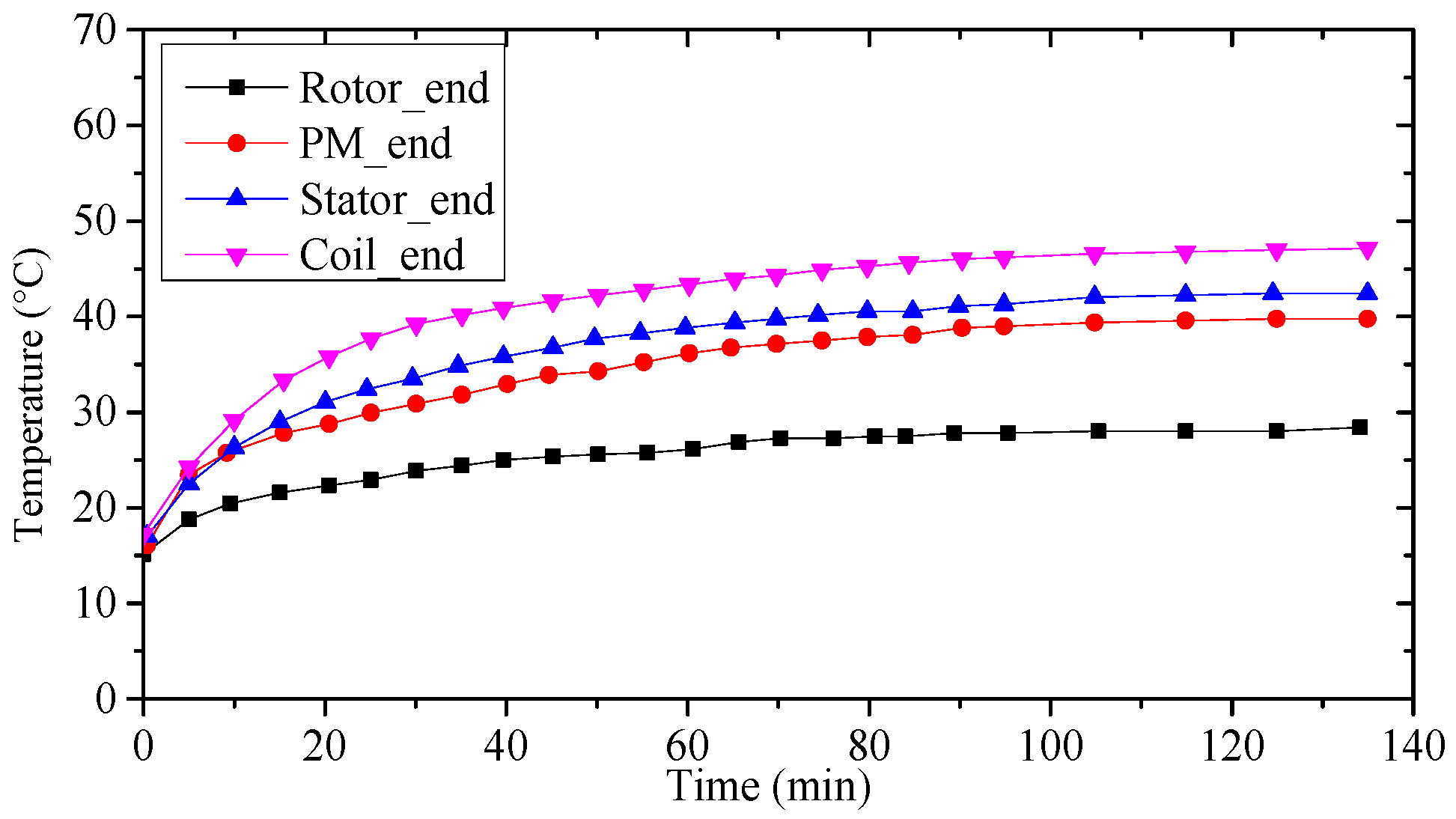
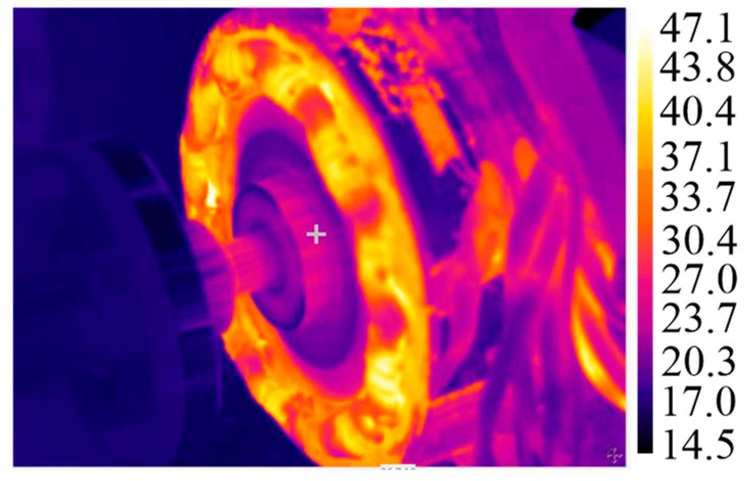
To verify the LPTN model, experiments on transient temperature rise were performed. Under the phase current of 30.7 A and rated speed of 1000 r/min, the transient temperature rises of different components under forced water cooling were obtained as shown in Figure 18, where the temperature was detected with a hand-held infrared thermometer. Under forced water-cooling conditions, the measured highest temperature was 47.1 °C. Compared with the results obtained by LPTN (Figure 9) and CFD (Figure 14), it was found that the steady-state and transient results of the three methods were very close. Figure 19 shows the experimental steady-state temperatures under forced water cooling. Obviously, agreement between the experiments and LPTN was achieved, validating the effectiveness of the LPTN model.

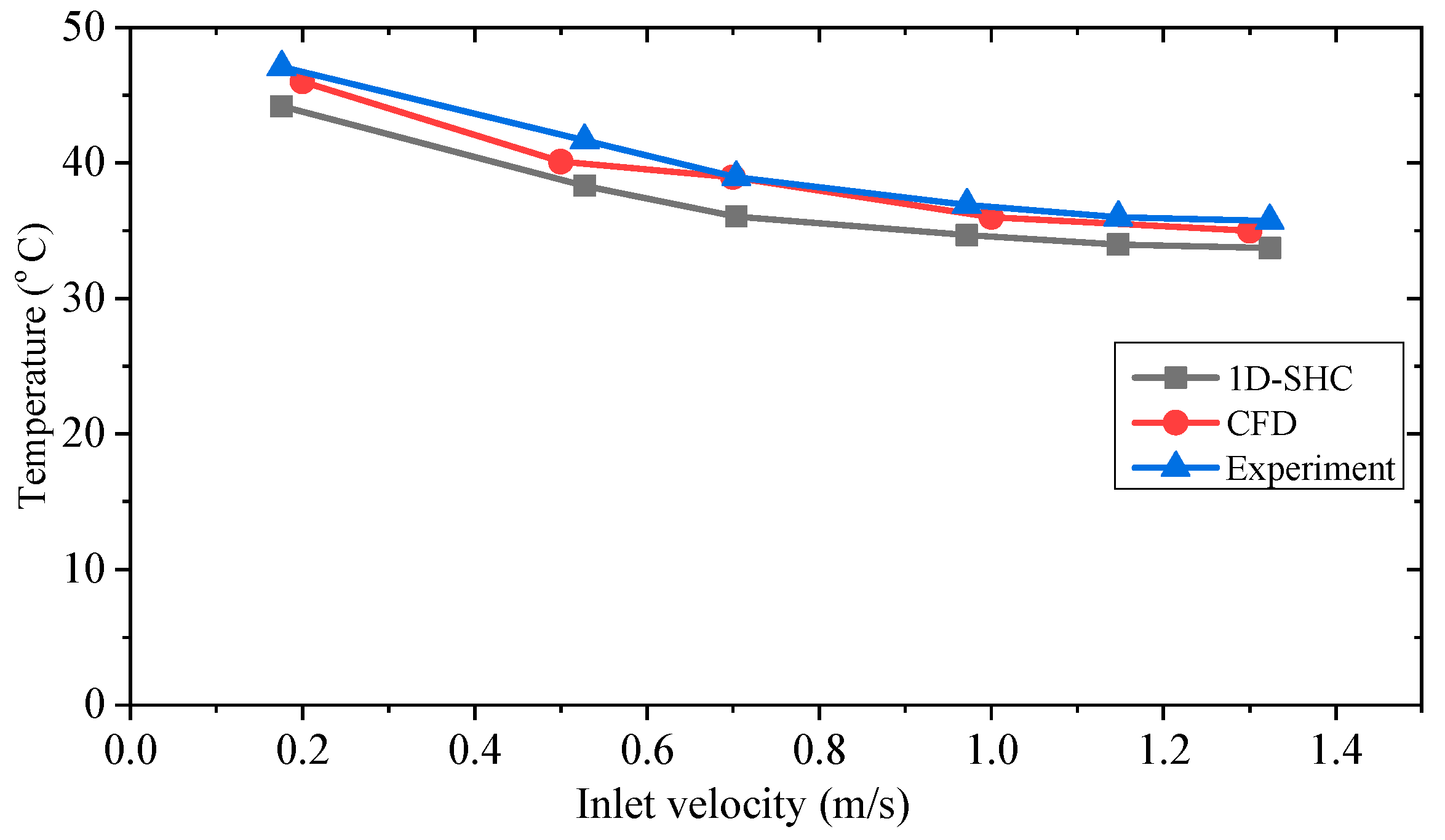
To verify the 1D-SHC model, experiments with temperature rising and various fluid inlet velocities of the no-load machine at the rated speed of 1000 r/min were conducted, as shown in Figure 20. It can be seen that when the inlet velocity was bigger than 1.1 m/s, the temperature of the equivalent stator core decreased slowly, which agrees with the simulations giving both 1D-SHC and CFD results.

Overall, satisfactory agreement was achieved between the calculation and measured results, considering manufacturing and testing tolerances.

6. Conclusions

In this paper, a LPTN model is constructed to predict transient thermal behavior of the FSPM machine. Meanwhile, a simplified 1D-SHC model is also proposed to obtain the relationship between the internal temperature of the stator and the coolant flow rate and coolant temperature. The time consumption of the LPTN and 1D-SHC models was significantly less than that of the CFD model, which has advantages in machine design and optimization with large amounts of data. Based on the housing water jacket cooling FSPM machine studied in this manuscript, the LPTN and 1D-SHC methods have accelerated the steady-state temperature calculation speed by 330 and 1100 times, respectively, compared to the CFD method, and have accelerated the transient calculation speed by 857 and 4285 times, respectively. The static and transient temperatures under different conditions were verified by the CFD calculations and experiments. The predicted results from the models agree well with experimental results. This work will be useful in further investigation of thermal analysis of FSPM machines.