

Energy-Optimal Speed Control for Autonomous Electric Vehicles Up- and Downstream of a Signalized Intersection
 , , and
Abstract
:1. Introduction
1.1. Context
1.2. Literature Review
- Incorporating the vehicle dynamics and time-dependent auxiliary consumption as a single objective function that accurately models the real-world situation.
- Implementation of a joint eco-approach-and-departure strategy to achieve a global optimum.
- Analytical parameterization of vehicle’s possible motion strategies to eliminate the time variable in the optimization.
2. Materials and Methods
2.1. Energy Consumption Modeling
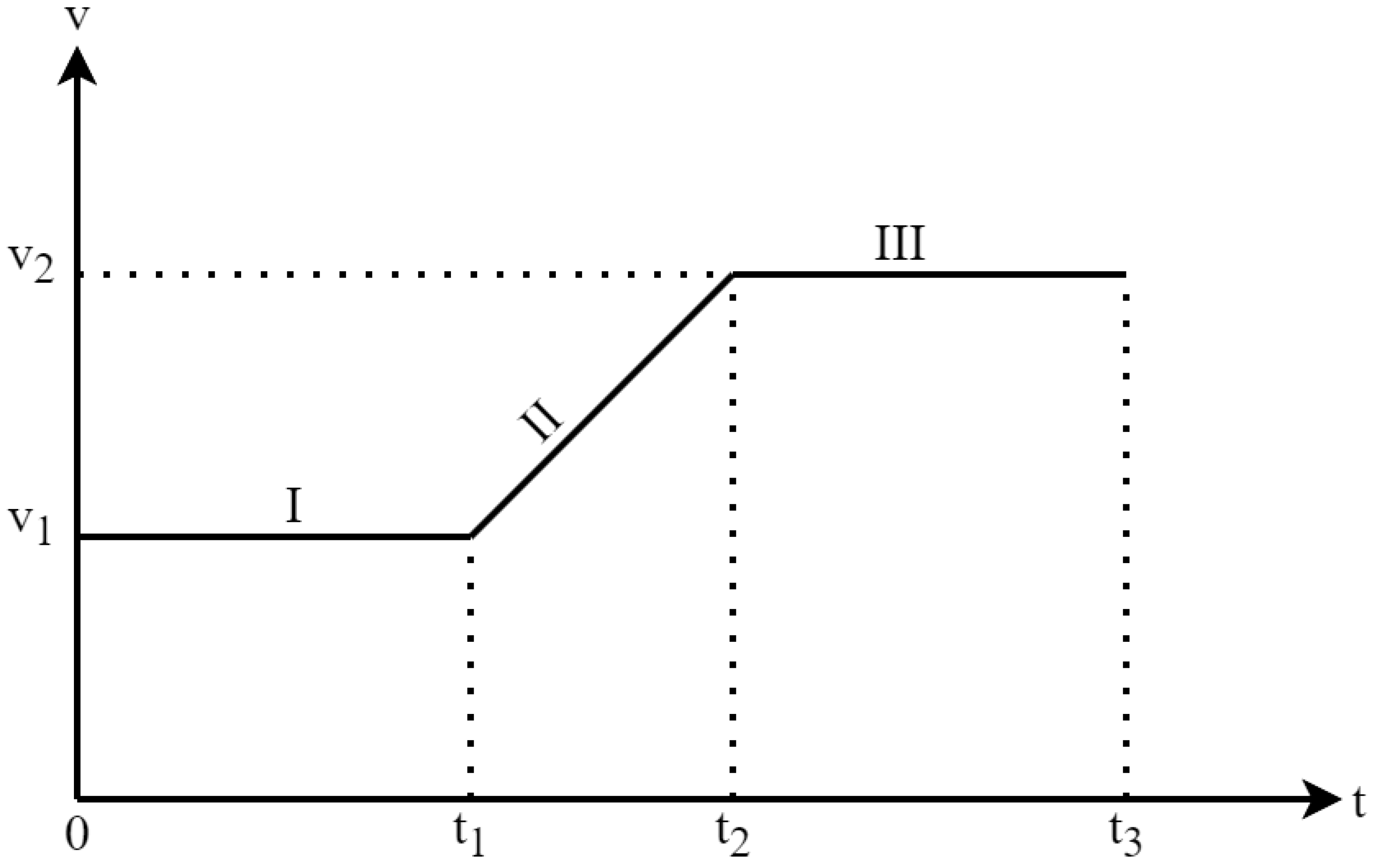
2.2. Energy Consumption Analytical Parameterization
- Cruise (C): Cruising with a constant speed over the whole trajectory.
- Accelerate (A): Accelerating or decelerating at a constant rate over the whole trajectory.
- Cruise–accelerate (C-A): First, cruising at a constant speed over a part of the trajectory; then, accelerating or decelerating with a constant rate over the remainder of the trajectory.
- Accelerate–cruise (A-C): First. accelerating or decelerating with a constant rate over a part of the trajectory; then, cruising with a constant speed over the remainder of the trajectory.
2.3. Eco-Ff Problem
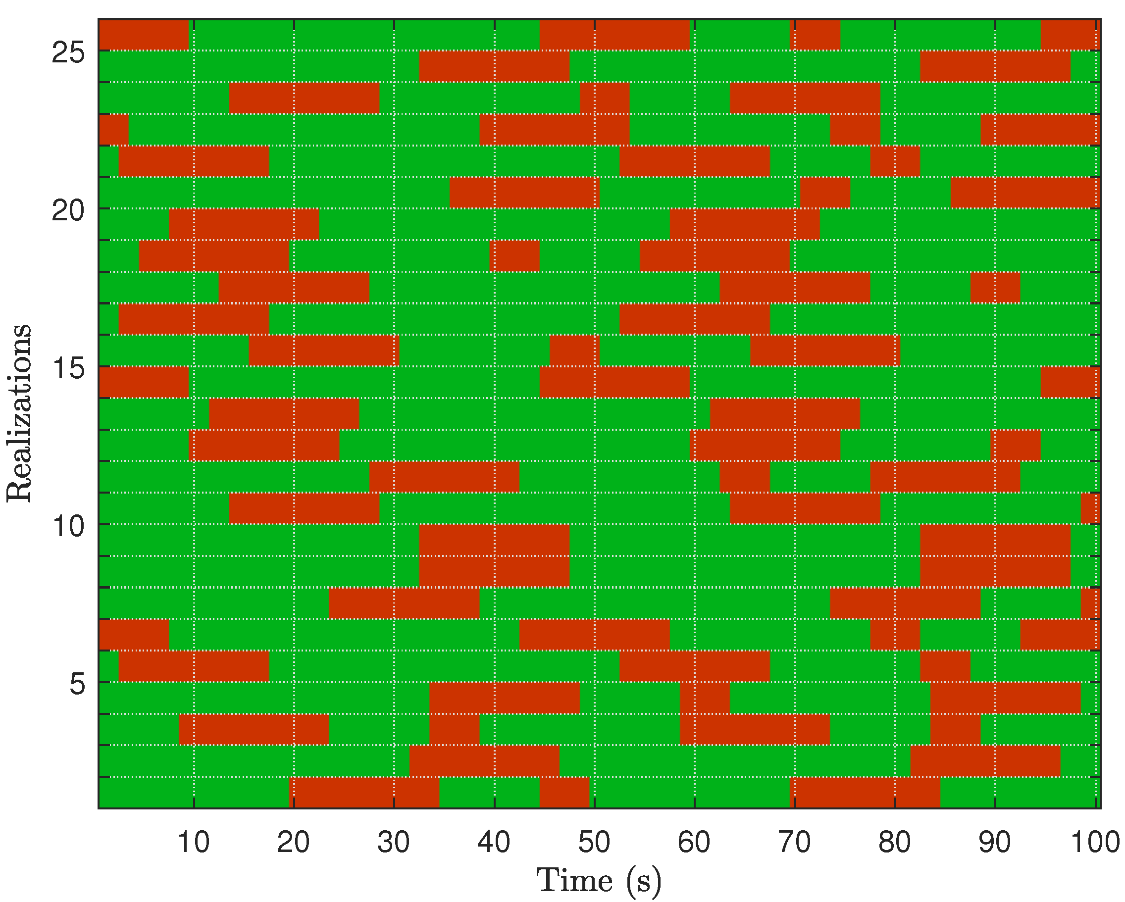
2.4. Human Driver Simulation
3. Results
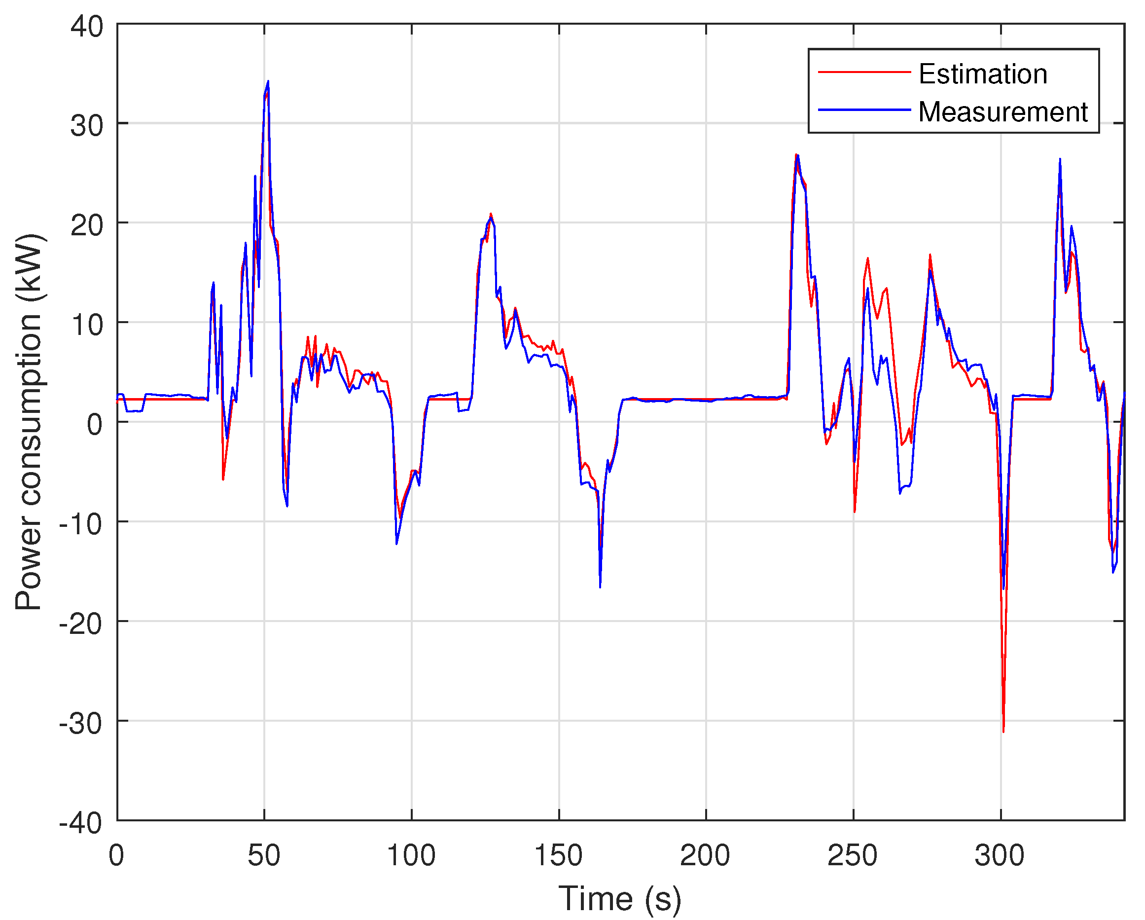
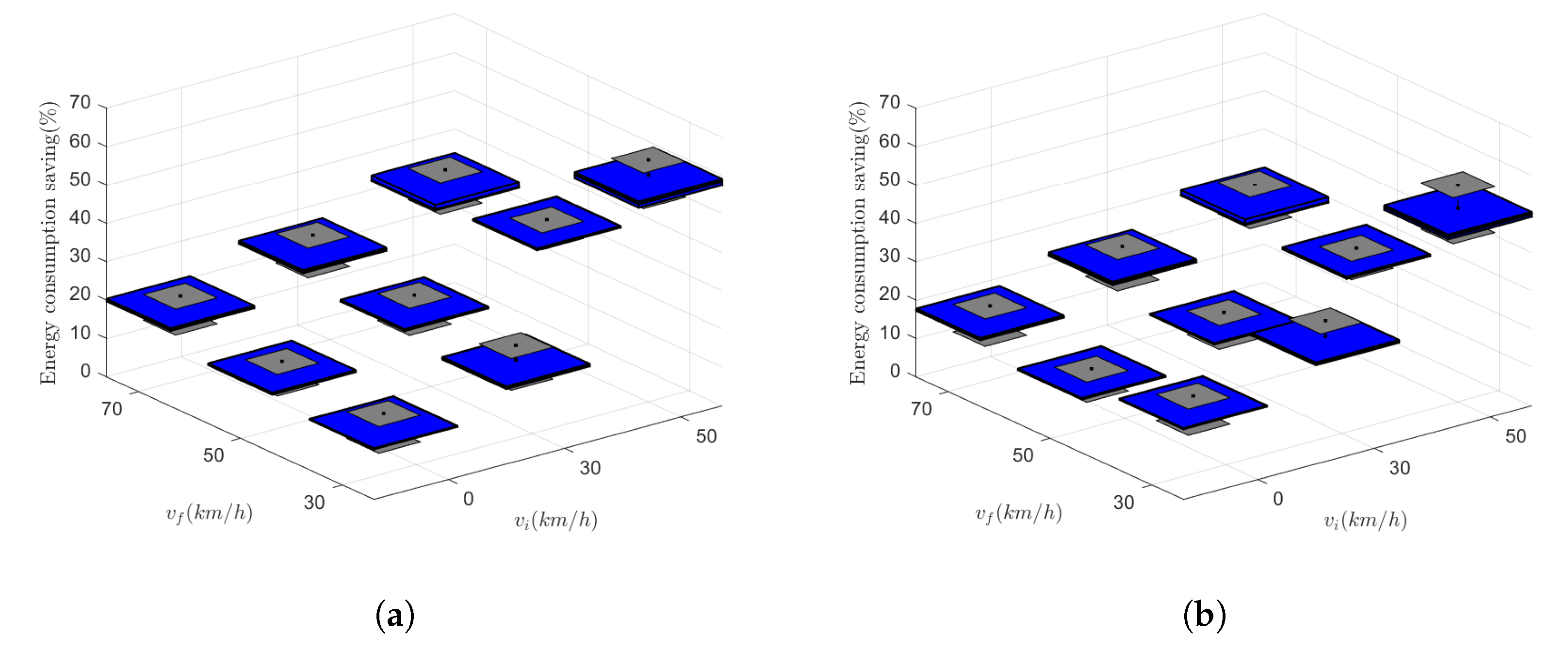
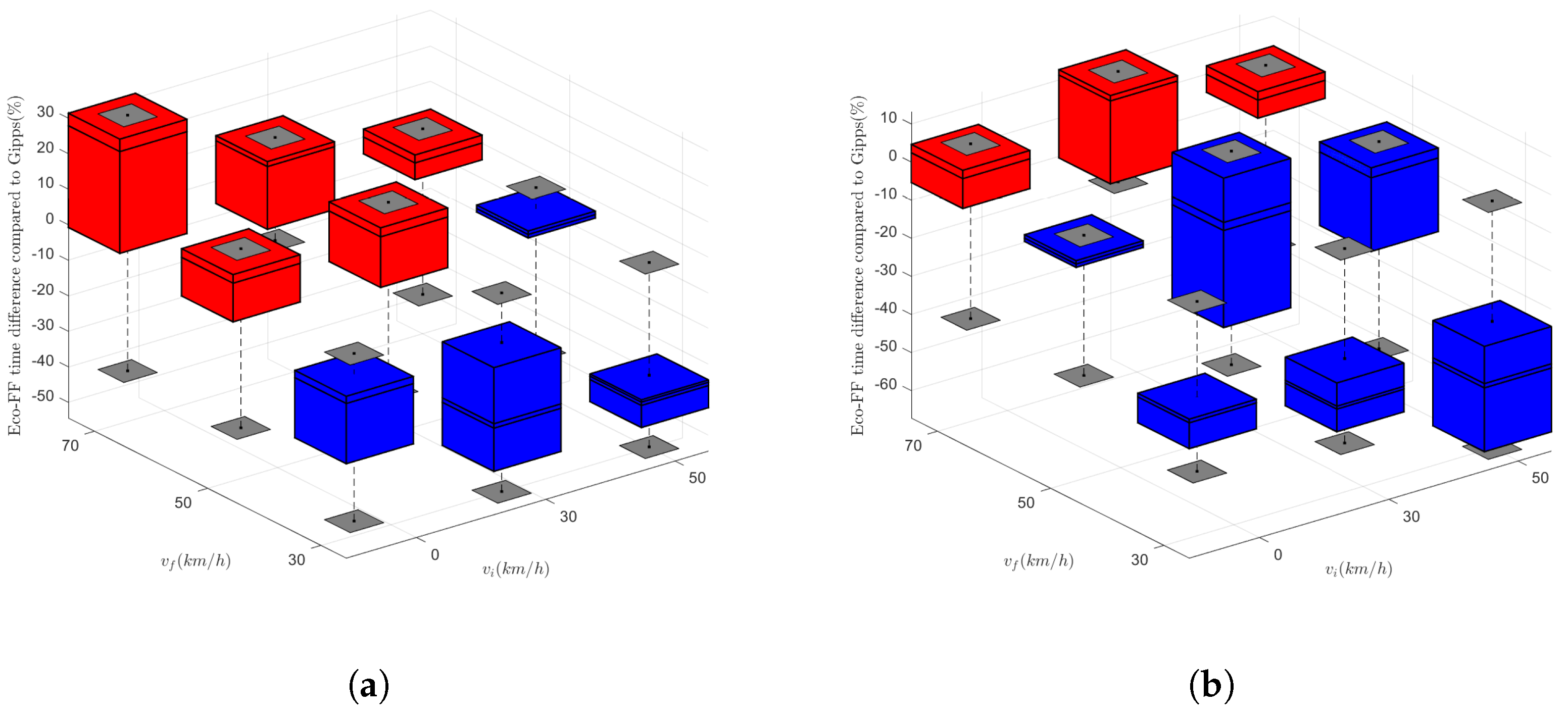
3.1. Measurement
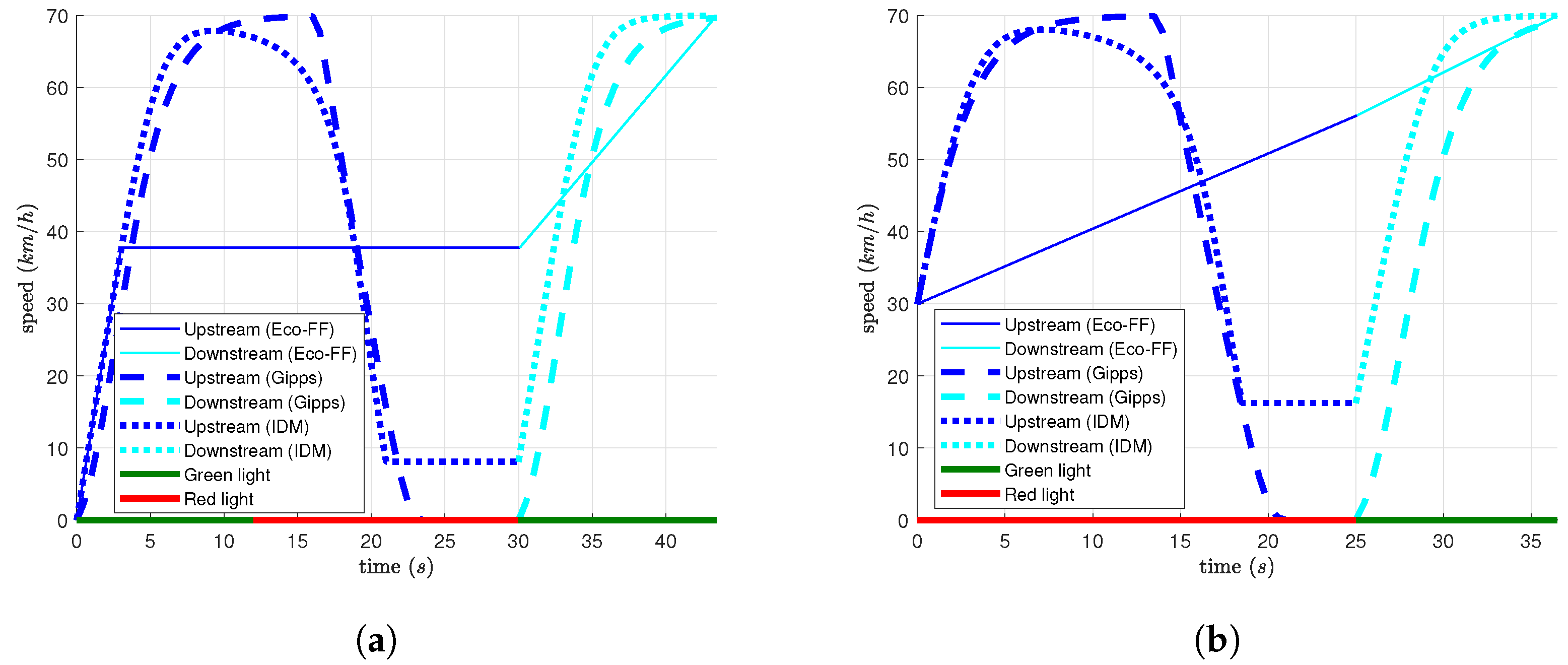
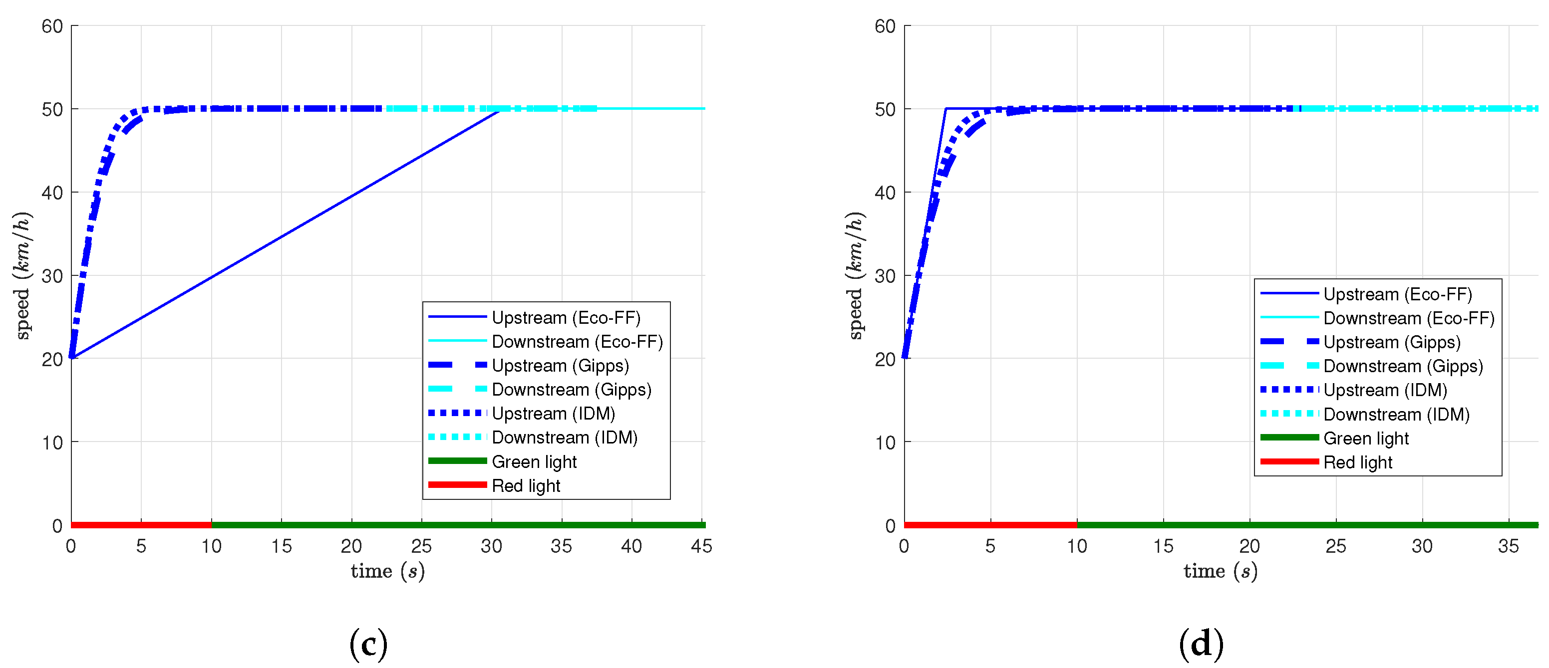
3.2. Results and Comparison
4. Conclusions
Author Contributions
Funding
Institutional Review Board Statement
Informed Consent Statement
Data Availability Statement
Conflicts of Interest
References
- Hao, P.; Wu, G.; Boriboonsomsin, K.; Barth, M.J. Eco-approach and departure (EAD) application for actuated signals in real-world traffic. IEEE Trans. Intell. Transp. Syst. 2018, 20, 30–40. [Google Scholar] [CrossRef] [Green Version]
- De Nunzio, G.; Gomes, G.; Canudas-de Wit, C.; Horowitz, R.; Moulin, P. Speed advisory and signal offsets control for arterial bandwidth maximization and energy consumption reduction. IEEE Trans. Control. Syst. Technol. 2016, 25, 875–887. [Google Scholar] [CrossRef] [Green Version]
- Xia, H.; Boriboonsomsin, K.; Schweizer, F.; Winckler, A.; Zhou, K.; Zhang, W.B.; Barth, M. Field operational testing of eco-approach technology at a fixed-time signalized intersection. In Proceedings of the 2012 15th International IEEE Conference on Intelligent Transportation Systems, Pittsburgh, PA, USA, 15–18 July 2012; pp. 188–193. [Google Scholar]
- Yang, H.; Almutairi, F.; Rakha, H. Eco-driving at signalized intersections: A multiple signal optimization approach. IEEE Trans. Intell. Transp. Syst. 2020, 22, 2943–2955. [Google Scholar] [CrossRef] [Green Version]
- Ma, F.; Yang, Y.; Wang, J.; Li, X.; Wu, G.; Zhao, Y.; Wu, L.; Aksun-Guvenc, B.; Guvenc, L. Eco-driving-based cooperative adaptive cruise control of connected vehicles platoon at signalized intersections. Transp. Res. Part Transp. Environ. 2021, 92, 102746. [Google Scholar] [CrossRef]
- Gilbert, E.G. Vehicle cruise: Improved fuel economy by periodic control. Automatica 1976, 12, 159–166. [Google Scholar] [CrossRef] [Green Version]
- Hooker, J.N. Optimal driving for single-vehicle fuel economy. Transp. Res. Part A Gen. 1988, 22, 183–201. [Google Scholar] [CrossRef]
- Hellström, E.; Åslund, J.; Nielsen, L. Design of an efficient algorithm for fuel-optimal look-ahead control. Control Eng. Pract. 2010, 18, 1318–1327. [Google Scholar] [CrossRef] [Green Version]
- Rakha, H.; Kamalanathsharma, R.K. Eco-driving at signalized intersections using V2I communication. In Proceedings of the 2011 14th International IEEE Conference on Intelligent Transportation Systems (ITSC), Washington, DC, USA, 5–7 October 2011; pp. 341–346. [Google Scholar]
- Ala, M.V.; Yang, H.; Rakha, H. Modeling evaluation of eco–cooperative adaptive cruise control in vicinity of signalized intersections. Transp. Res. Rec. 2016, 2559, 108–119. [Google Scholar] [CrossRef]
- Jiang, H.; Hu, J.; An, S.; Wang, M.; Park, B.B. Eco approaching at an isolated signalized intersection under partially connected and automated vehicles environment. Transp. Res. Part Emerg. Technol. 2017, 79, 290–307. [Google Scholar] [CrossRef]
- Yang, H.; Rakha, H.; Ala, M.V. Eco-cooperative adaptive cruise control at signalized intersections considering queue effects. IEEE Trans. Intell. Transp. Syst. 2016, 18, 1575–1585. [Google Scholar] [CrossRef]
- Mandava, S.; Boriboonsomsin, K.; Barth, M. Arterial velocity planning based on traffic signal information under light traffic conditions. In Proceedings of the 2009 12th International IEEE Conference on Intelligent Transportation Systems, St. Louis, MO, USA, 4–7 October 2009; pp. 1–6. [Google Scholar]
- Barth, M.; Mandava, S.; Boriboonsomsin, K.; Xia, H. Dynamic ECO-driving for arterial corridors. In Proceedings of the 2011 IEEE Forum on Integrated and Sustainable Transportation Systems, Vienna, Austria, 29 June–1 July 2011; pp. 182–188. [Google Scholar]
- HomChaudhuri, B.; Vahidi, A.; Pisu, P. A fuel economic model predictive control strategy for a group of connected vehicles in urban roads. In Proceedings of the 2015 American Control Conference (ACC), Chicago, IL, USA, 1–3 July 2015; pp. 2741–2746. [Google Scholar]
- Wang, Z.; Wu, G.; Hao, P.; Boriboonsomsin, K.; Barth, M. Developing a platoon-wide eco-cooperative adaptive cruise control (CACC) system. In Proceedings of the 2017 Ieee Intelligent Vehicles Symposium (iv), Los Angeles, CA, USA, 11–14 June 2017; pp. 1256–1261. [Google Scholar]
- Asadi, B.; Vahidi, A. Predictive cruise control: Utilizing upcoming traffic signal information for improving fuel economy and reducing trip time. IEEE Trans. Control. Syst. Technol. 2010, 19, 707–714. [Google Scholar] [CrossRef]
- Mahler, G.; Vahidi, A. Reducing idling at red lights based on probabilistic prediction of traffic signal timings. In Proceedings of the 2012 American Control Conference (ACC), Montreal, QC, Canada, 27–29 June 2012; pp. 6557–6562. [Google Scholar]
- Mahler, G.; Vahidi, A. An optimal velocity-planning scheme for vehicle energy efficiency through probabilistic prediction of traffic-signal timing. IEEE Trans. Intell. Transp. Syst. 2014, 15, 2516–2523. [Google Scholar] [CrossRef]
- Chen, P.; Yan, C.; Sun, J.; Wang, Y.; Chen, S.; Li, K. Dynamic eco-driving speed guidance at signalized intersections: Multivehicle driving simulator based experimental study. J. Adv. Transp. 2018, 2018, 6031764. [Google Scholar] [CrossRef]
- Oh, G.; Peng, H. Eco-driving at signalized intersections: What is possible in the real-world? In Proceedings of the 2018 21st International Conference on Intelligent Transportation Systems (ITSC), Maui, HI, USA, 4–7 November 2018; pp. 3674–3679. [Google Scholar]
- Sun, C.; Guanetti, J.; Borrelli, F.; Moura, S.J. Optimal eco-driving control of connected and autonomous vehicles through signalized intersections. IEEE Internet Things J. 2020, 7, 3759–3773. [Google Scholar] [CrossRef]
- Kamalanathsharma, R.K.; Rakha, H.A. Multi-stage dynamic programming algorithm for eco-speed control at traffic signalized intersections. In Proceedings of the 16th International IEEE Conference on Intelligent Transportation Systems (ITSC 2013), The Hague, The Netherlands, 6–9 October 2013; pp. 2094–2099. [Google Scholar]
- Mousa, S.R.; Ishak, S.; Mousa, R.M.; Codjoe, J. Developing an eco-driving application for semi-actuated signalized intersections and modeling the market penetration rates of eco-driving. Transp. Res. Rec. 2019, 2673, 466–477. [Google Scholar] [CrossRef]
- Tang, T.Q.; Yi, Z.Y.; Zhang, J.; Wang, T.; Leng, J.Q. A speed guidance strategy for multiple signalized intersections based on car-following model. Phys. A Stat. Mech. Its Appl. 2018, 496, 399–409. [Google Scholar] [CrossRef]
- Han, J.; Vahidi, A.; Sciarretta, A. Fundamentals of energy efficient driving for combustion engine and electric vehicles: An optimal control perspective. Automatica 2019, 103, 558–572. [Google Scholar] [CrossRef]
- De Nunzio, G.; De Wit, C.C.; Moulin, P.; Di Domenico, D. Eco-driving in urban traffic networks using traffic signals information. Int. J. Robust Nonlinear Control 2016, 26, 1307–1324. [Google Scholar] [CrossRef] [Green Version]
- Zhang, J.; Tang, T.Q.; Yan, Y.; Qu, X. Eco-driving control for connected and automated electric vehicles at signalized intersections with wireless charging. Appl. Energy 2021, 282, 116215. [Google Scholar] [CrossRef]
- Boyd, S.; Boyd, S.P.; Vandenberghe, L. Convex Optimization; Cambridge University Press: Cambridge, UK, 2004. [Google Scholar]
- Gipps, P.G. A behavioural car-following model for computer simulation. Transp. Res. Part B Methodol. 1981, 15, 105–111. [Google Scholar] [CrossRef]
- Kesting, A.; Treiber, M.; Helbing, D. Enhanced intelligent driver model to access the impact of driving strategies on traffic capacity. Philos. Trans. R. Soc. Math. Phys. Eng. Sci. 2010, 368, 4585–4605. [Google Scholar] [CrossRef] [PubMed] [Green Version]
- Available online: https://www.press.bmwgroup.com/global/article/attachment/T0284828EN/415571 (accessed on 18 December 2022).
- Asamer, J.; Graser, A.; Heilmann, B.; Ruthmair, M. Sensitivity analysis for energy demand estimation of electric vehicles. Transp. Res. Part D Transp. Environ. 2016, 46, 182–199. [Google Scholar] [CrossRef]


| Strategy | |||
|---|---|---|---|
| C | 0 | 0 | |
| A | 0 | ||
| C-A | |||
| A-C | 0 |
| Parameter | Value | Parameter | Value |
|---|---|---|---|
| Driveline efficiency: | Frontal area: | 2.38 (m2) | |
| Regenerative efficiency: | Vehicle’s mass: m | 1270 (Kg) | |
| Rotating parts’ mass factor: | Upstream distance: | 300 (m) | |
| Friction coefficient: | Downstream distance: | 200 (m) | |
| Gravitational acceleration: g | (m/s2) | Min. acceleration: | (m/s2) |
| Air density: | (Kg/m3) | Max. acceleration: | (m/s2) |
| Air drag coefficient: | Max. speed limit: | 70 (km/h) |
Disclaimer/Publisher’s Note: The statements, opinions and data contained in all publications are solely those of the individual author(s) and contributor(s) and not of MDPI and/or the editor(s). MDPI and/or the editor(s) disclaim responsibility for any injury to people or property resulting from any ideas, methods, instructions or products referred to in the content. |
© 2023 by the authors. Licensee MDPI, Basel, Switzerland. This article is an open access article distributed under the terms and conditions of the Creative Commons Attribution (CC BY) license (https://creativecommons.org/licenses/by/4.0/).
Share and Cite
Hesami, S.; De Cauwer, C.; Rombaut, E.; Vanhaverbeke, L.; Coosemans, T. Energy-Optimal Speed Control for Autonomous Electric Vehicles Up- and Downstream of a Signalized Intersection. World Electr. Veh. J. 2023, 14, 55. https://doi.org/10.3390/wevj14020055
Hesami S, De Cauwer C, Rombaut E, Vanhaverbeke L, Coosemans T. Energy-Optimal Speed Control for Autonomous Electric Vehicles Up- and Downstream of a Signalized Intersection. World Electric Vehicle Journal. 2023; 14(2):55. https://doi.org/10.3390/wevj14020055
Chicago/Turabian StyleHesami, Simin, Cedric De Cauwer, Evy Rombaut, Lieselot Vanhaverbeke, and Thierry Coosemans. 2023. "Energy-Optimal Speed Control for Autonomous Electric Vehicles Up- and Downstream of a Signalized Intersection" World Electric Vehicle Journal 14, no. 2: 55. https://doi.org/10.3390/wevj14020055