
PerfECT Design Tool: Electric Vehicle Modelling and Experimental Validation


Abstract
:1. Introduction
2. Modelling Theoretical Background
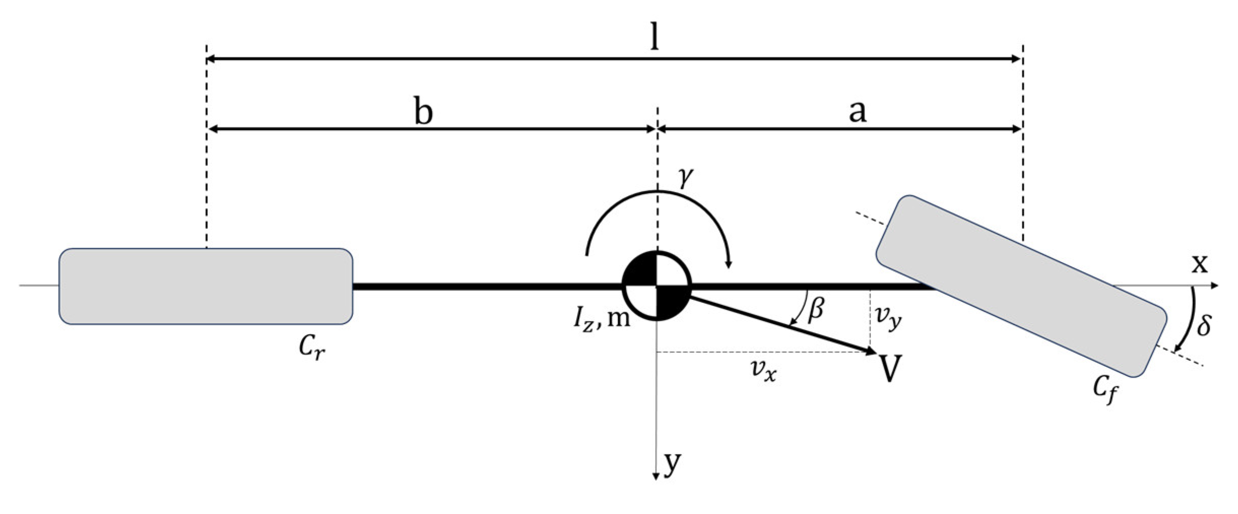
2.1. Lateral Dynamics Modelling
2.2. Longitudinal Dynamics Modelling
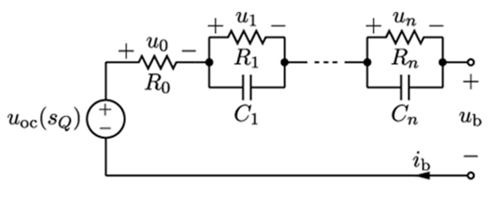
2.3. Batteries
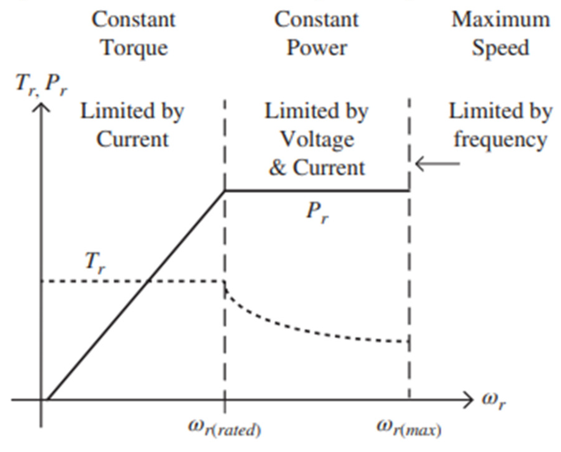
2.4. Electric Powertrain
- In the case of SPM machines, the disposition of the magnets in the rotor is isotropic, thus the terms , while the flux generated by the PMs is aligned with the d-axis so while ;
- For IPM the situation is equivalent regarding the PM flux, but the disposition of the PM is anisotropic, and made so that ;
- In the case of RM, the form of the rotor is such that the contribution of the inductances is much more influential in the d-axis, thus , while no PM is included, so that ;
- For PM–SyR machines it remains true that ; however, the presence of PMs in the structure means that the contribution is while .
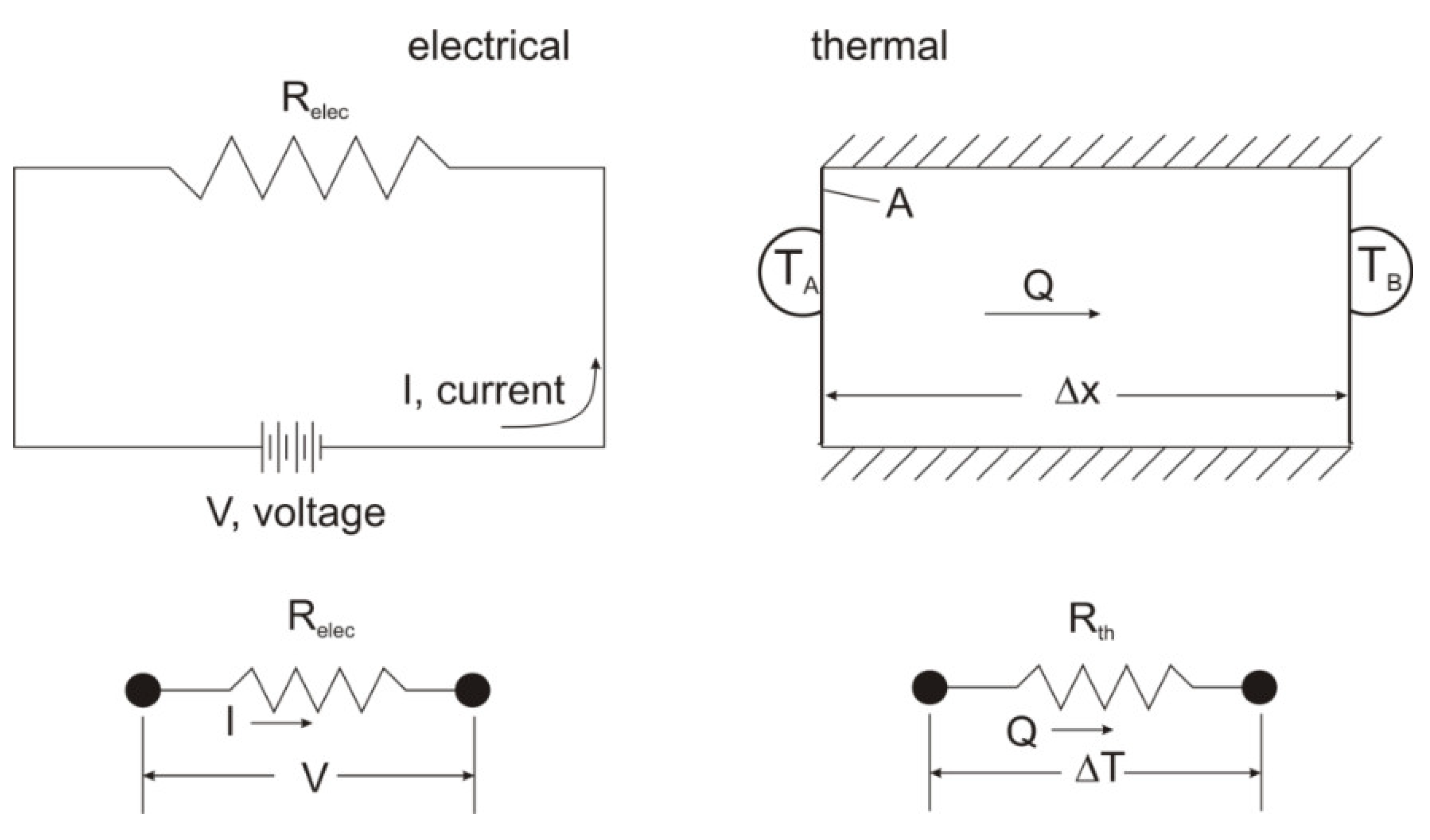
2.5. Thermal Modelling
- Internal resistance: with the current flows in the battery pack, it is possible to determine the resistance contribution to the total energy loss and consequent heat generation. In the case of a constant current discharge, the heat generated can be expressed as:
- Chemical reactions: as is known, during the release or absorption of energy from/to the battery, chemical reactions take place. Apart from the electric equilibrium that represents the main mechanism of the chemical battery, these reactions also play a role in terms of heat generation. The heat associated with the chemical reaction can be derived by:
3. The PerfECT Design Tool Implementation
3.1. The Four-Level Concept
- Performance level: this level reflects the very beginning of the conceptual study of the vehicle, in which the only readily available information and “fixed” features are the ones decided in the requirements definition and registered in the product requirement document. This stage then focuses on the “reality check” of the desired performance, an evaluation of possible layouts for the powertrain, and a first broad procurement phase on E-PWT components, more specifically at this stage in terms of electric machines. It naturally follows that, in such an analysis, only the very essential vehicle parameters can be requested, and only very simple outcomes can be reliably expected;
- Energy level: as with the previous step, the energy level proposes a simple and quick modeling structure, focusing on the longitudinal dynamics response of the vehicle and adding information regarding the energy flow. When it comes to energy evaluation, the main additional information provided to the system are the curves of the e-motors (usually available from suppliers’ datasheet) and information regarding battery capacity, energy management and the regenerative braking strategy. From this analysis, it is possible to extract some vital features for EVs, such as their expected range, and therefore also adjust parameters to increase/optimize them;
- Currents level: the gap between the energy level and currents level is probably the widest among the sequences; in order to successfully evaluate currents flowing in the high-voltage circuits of an E-PWT, it is necessary to significantly increase the complexity of the electric machine modeling and their correlated components. From this level on, the lateral dynamics simulation platform is also optionally integrated, in such a way that the designer can expand the analysis from pure drivability to include handling and stability analyses;
- Temperature level: as the final stage of the concept phase in product development, this level adds an important number of parameters to the analysis related to thermal characteristics. To correctly evaluate the temperature variations on the vehicle components, it is essential to understand the heat generation, heat transfer, and cooling loop features; each one of these is based on several hypotheses and parameters. The goal of the tool is not to substitute specialized thermal modeling software; therefore, a geometry-less approach was used in which the physical disposition and connections among parts is represented by lumped thermal exchange resistances. This approach allows for the PerfECT tool to be used as a target-setting instrument and as an interface with detailed CFD and multi-physics analysis.
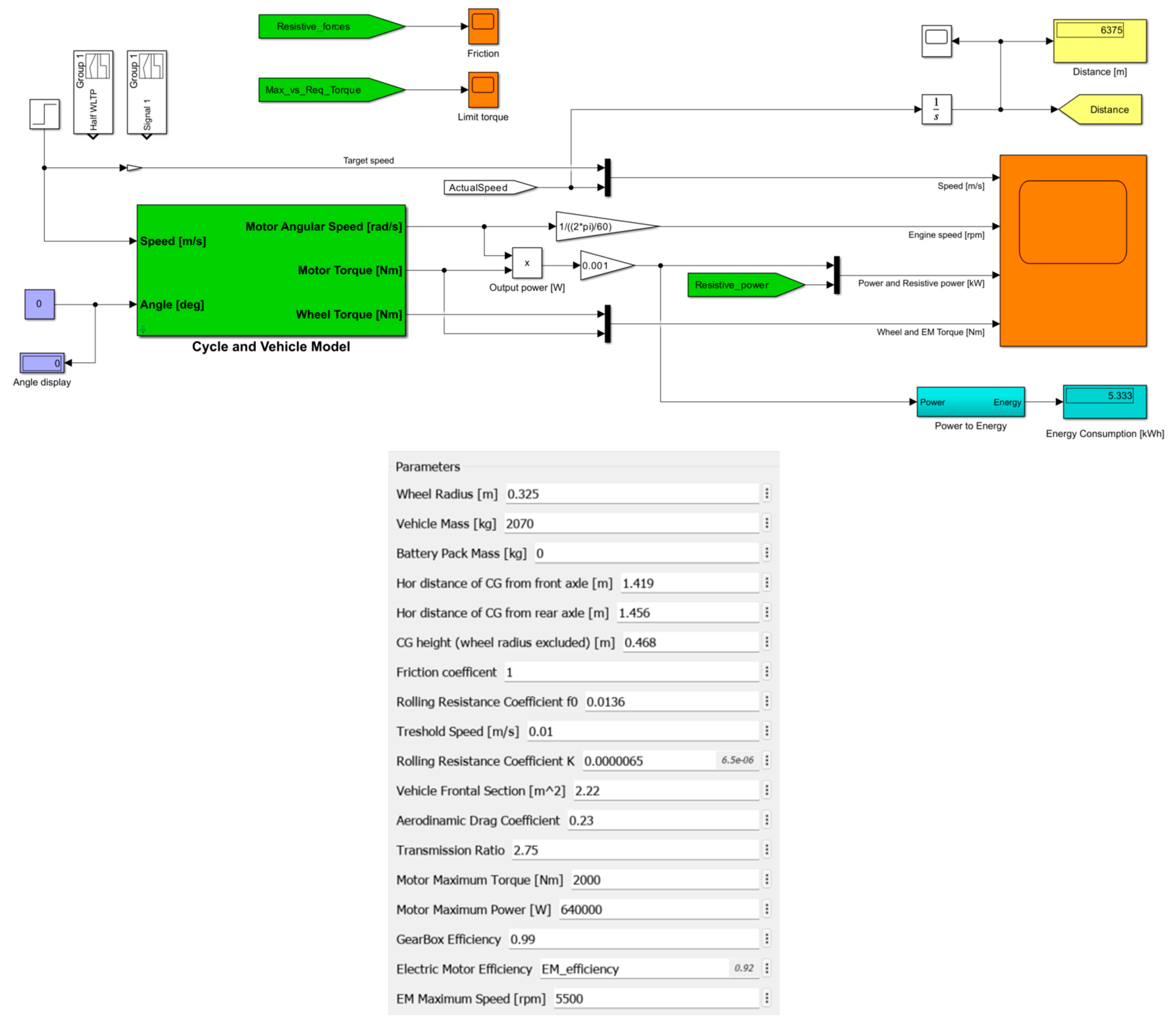
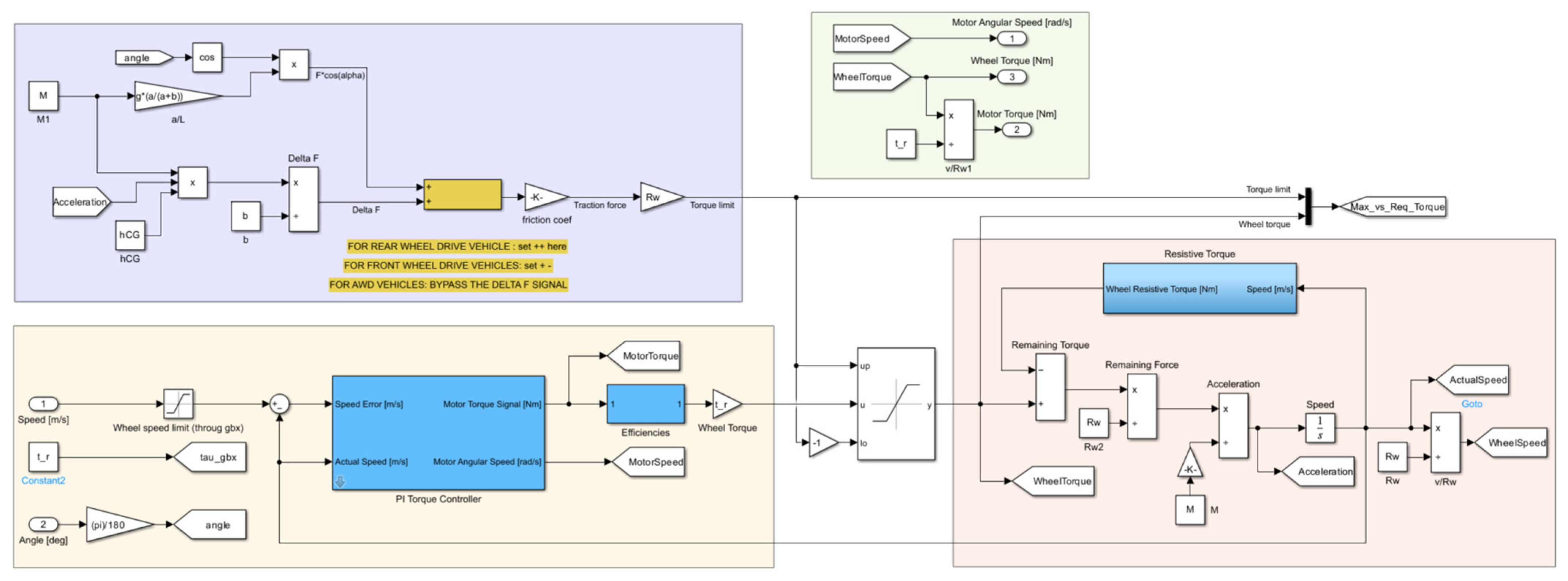
3.2. Performance Level
- Blue: calculates the maximum traction that the tires can transmit to the road due to the friction coefficient, mass, slope, and longitudinal load transfer (hCG and acceleration);
- Yellow: compares the actual speed and the target in the desired profile and chooses the adequate wheel torque request using a PI controller;
- Red: receives the saturated torque request and calculates the resistive torque based on the vehicle speed, thereby obtaining the residual acceleration, and integrating it to obtain the next timestep velocity;
- Green: recalls and calculates the block outputs—motor angular speed, wheel torque and motor torque.
- WOT acceleration: by imposing a very high target velocity from the beginning of the simulation, it is possible to determine the time evolution of speed under maximum torque request. The acceleration is limited by EM features, friction, inertia, and resistive forces, which can be tuned and tweaked to achieve design goals as 0–100 km/h time;
- Maximum slope: by interactively increasing the slope angle input, it is possible to analyze the vehicle response on design criteria such as maximum gradeability or minimum speed/acceleration in pre-determined slope conditions;
- Maximum speed: it is possible to numerically determine the maximum speed achievable by the vehicle. Like the WOT analysis, it can be done by setting a high value of target speed and forcing the system to give all available power/torque in such a way that the speed will tend to the maximum obtainable value. The limit can be due to torque/power of the EM being counterposed by the resistances or due to a motor speed limit;
- Residual acceleration: at any given operation point, the system can be used to evaluate the total resistive power and compare it with the peak values of the powertrain to determine the available residual power that can be exploited for acceleration.
3.3. Energy Level
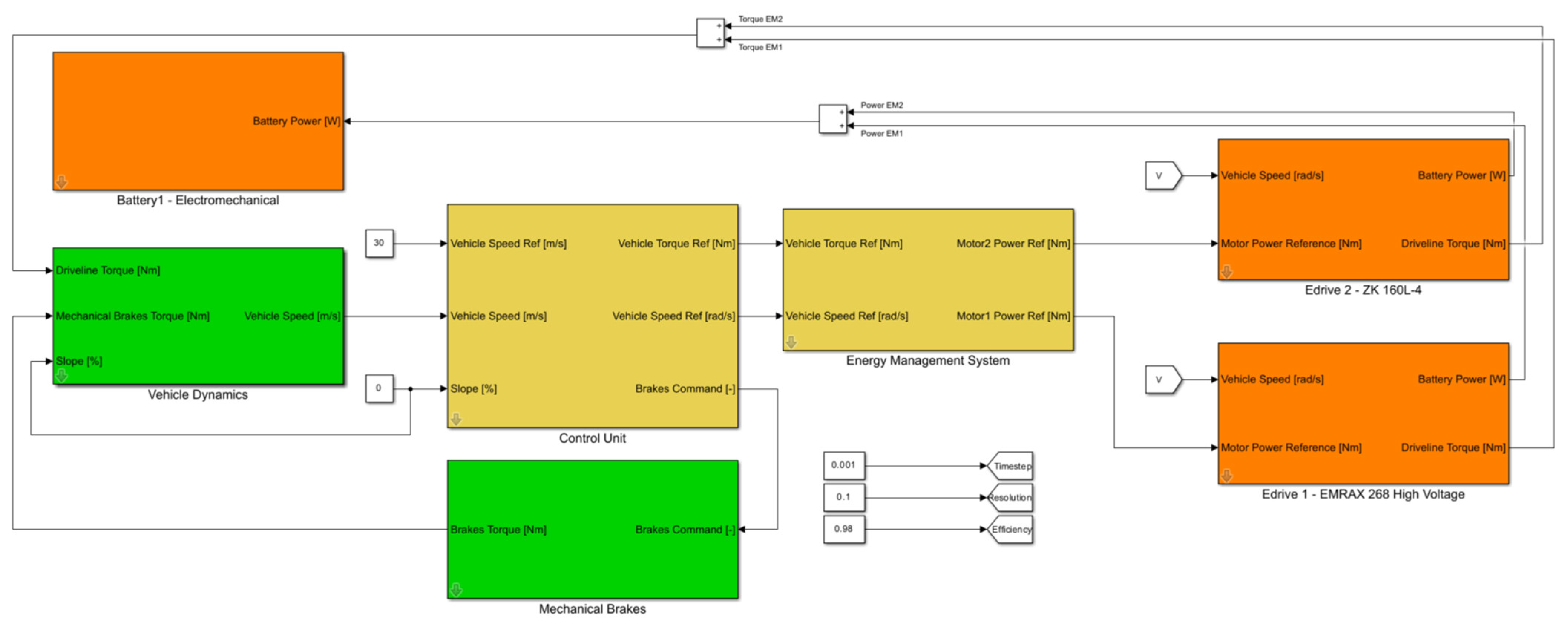
3.4. Currents Level
- Control Unit: this subsystem is responsible for translating the input desired speed profile and transforming it into a torque request to the E-PWT and mechanical brakes. It encompasses, basically, the PI controller and the regenerative braking controller from the “Energy” level. The main difference, in this case, is that the “Motor Torque Reference Generator”, responsible for the translation of 0–100% acceleration signals into torques, considers the saturations coming from different sources. The torque limits, power limits and speed limits come from the signals in the EM models, taking into consideration not only the peak or continuous values present in the EM datasheets, but also the logic of over-torque, over-power and over-speed and their maximum allowable times;
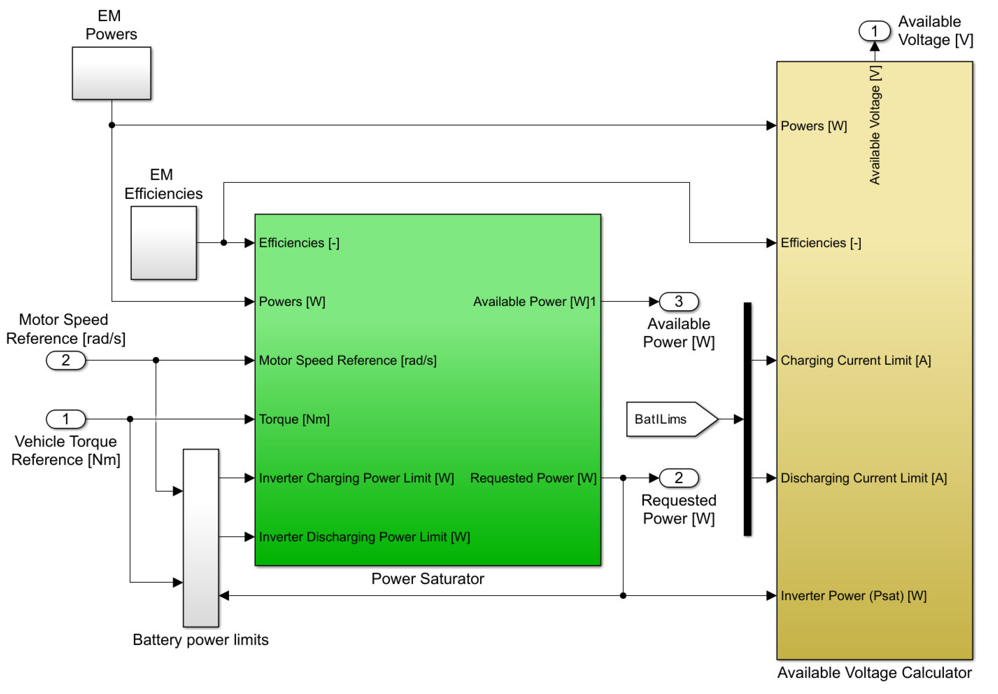
- Energy management system: this subsystem is responsible for translating the total torque request coming from the controller into a torque command for each motor in the E-PWT. The first step is to perform further saturation, by inquiring the maximum power and voltage available at the battery level (Figure 8).
- Inverter: converts the torque request into output Vd and Vq signals and motor status, after saturating the torque request with the maximum flux, available voltage, and information regarding the overloads. Using the MTPA maps this block converts reference EM torque into Id and Iq minimum currents to achieve such torque, then through the physical model they are used to determine the voltages;
- Overload management: is composed of three smaller blocks, each one responsible for keeping track of one of the following key overload behaviors: Torque, Power and Speed. The overload state is characterized by an output that lies between the continuous reference and the peak reference. Obviously, it is not possible for the EM to maintain a peak performance indefinitely, so these controllers determine when to return to the continuous value after some time in overload. The method used to do so is based on a “StateFlow” module in Simulink, where an energetic approach is implemented. The basic idea is that each instant the system is over the continuous value, it is accumulating energy that will then be turned into heat and compromise long-term performance. Once the energy level is too high—based on supplier indications—StateFlow takes it back to the continuous level until the accumulated heat has not dissipated. The same outline is used for the three overload behaviors;
- Motor electro-mechanical model: this block is a straightforward implementation of the equivalent circuit equations in the d-q axis EM model. From them, the real output torque can be calculated, modeling the internal fluxes and EM dynamics. The electromagnetic power needed to perform this operating point load can also be determined;
- Driveline: the last block determines the share of the power that shall not be available to create useful mechanical torque, due to internal losses and inefficiencies (as well as the extra power requested to the storage system). Here, the copper losses, iron losses, bearing losses, aerodynamic losses, and inertial counter-torque are estimated.
3.5. Temperature Level
- Ambient temperature;
- Initial temperature of each part;
- Cooling fluid volume, density and heat capacity;
- Radiator dimensions and efficiency;
- Cooling circuit flow rate and distribution among components.
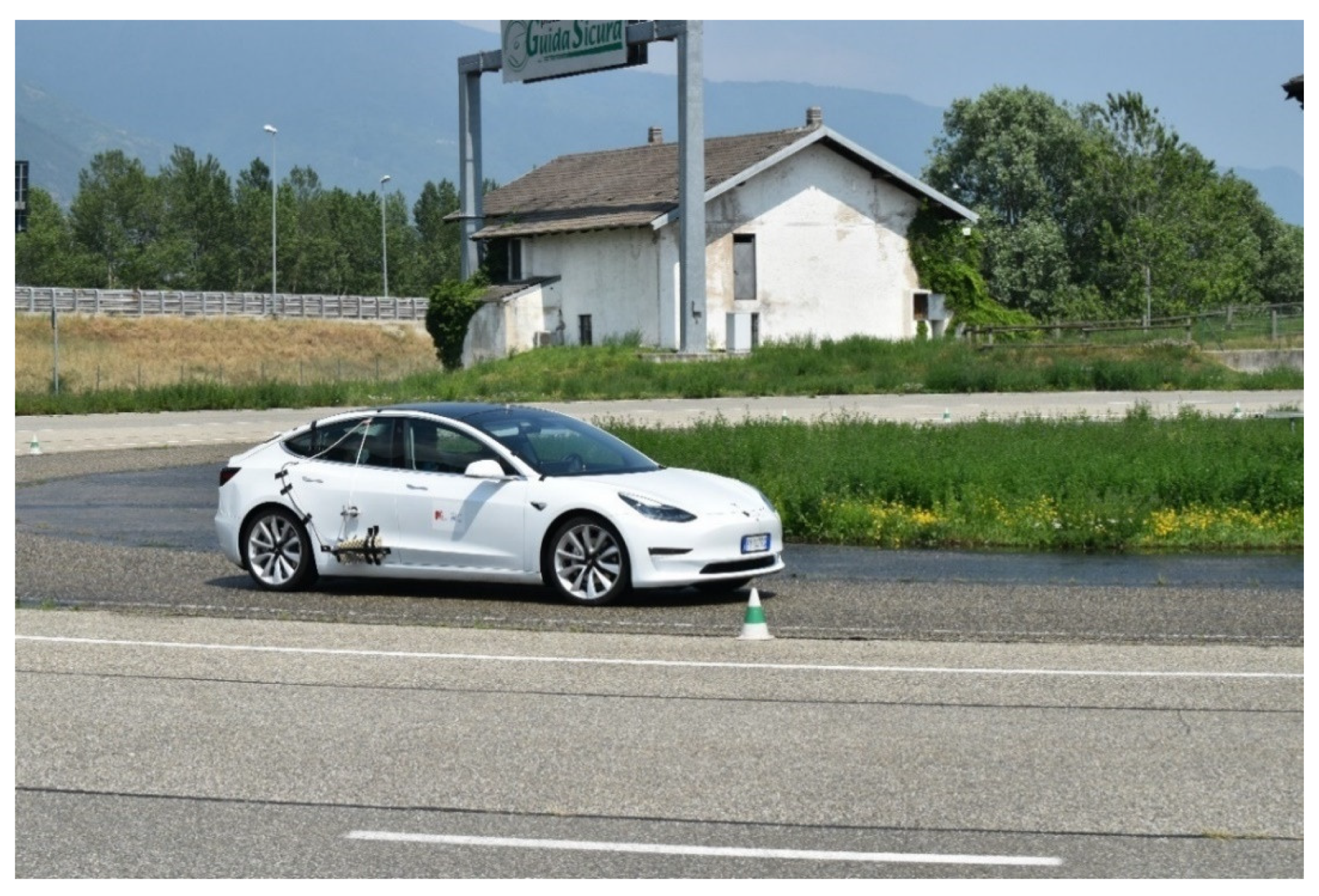
4. Practical Validation on a Tesla Model 3
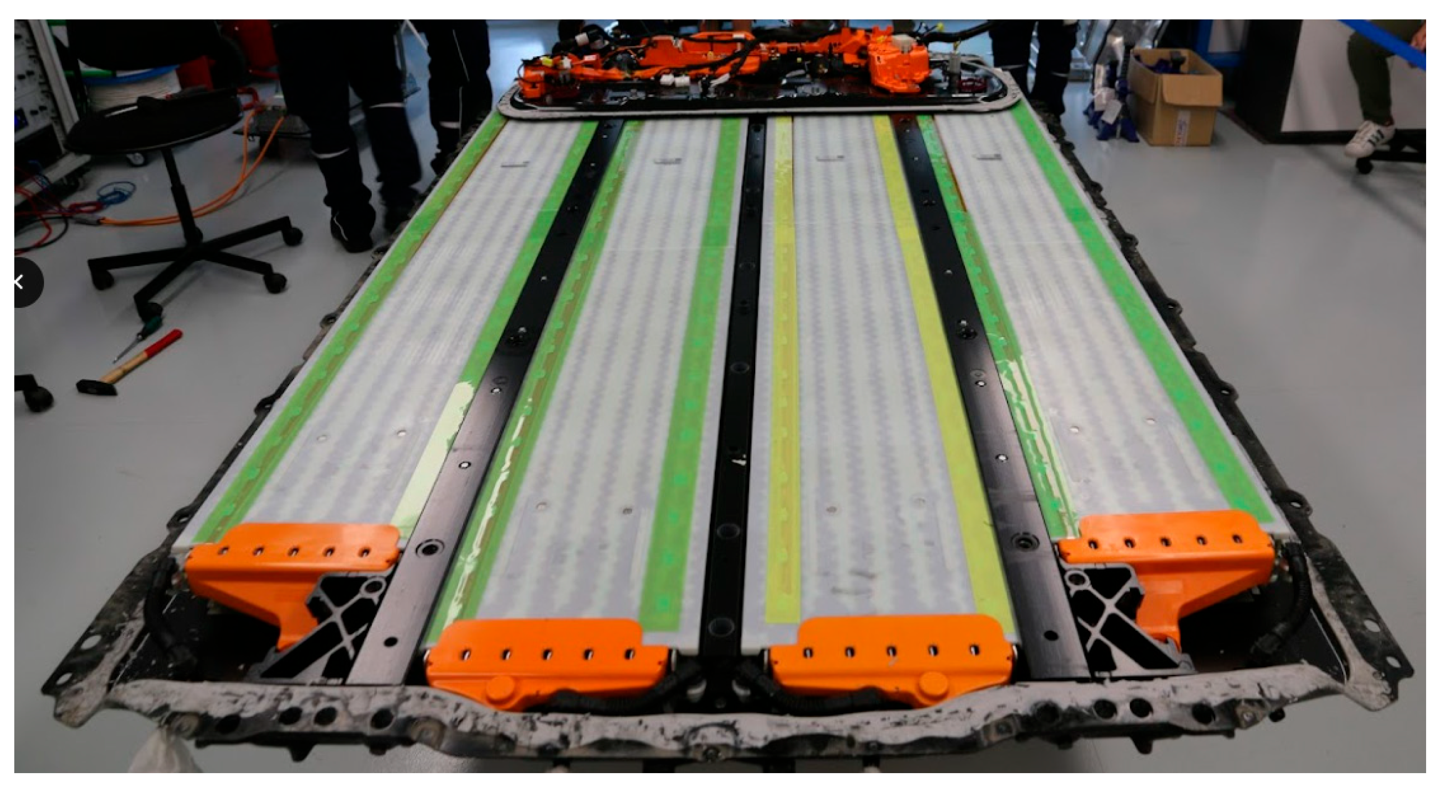
4.1. The Vehicle
- 23 series and 46 parallel for the external modules;
- 25 series and 46 parallel for the internal modules.
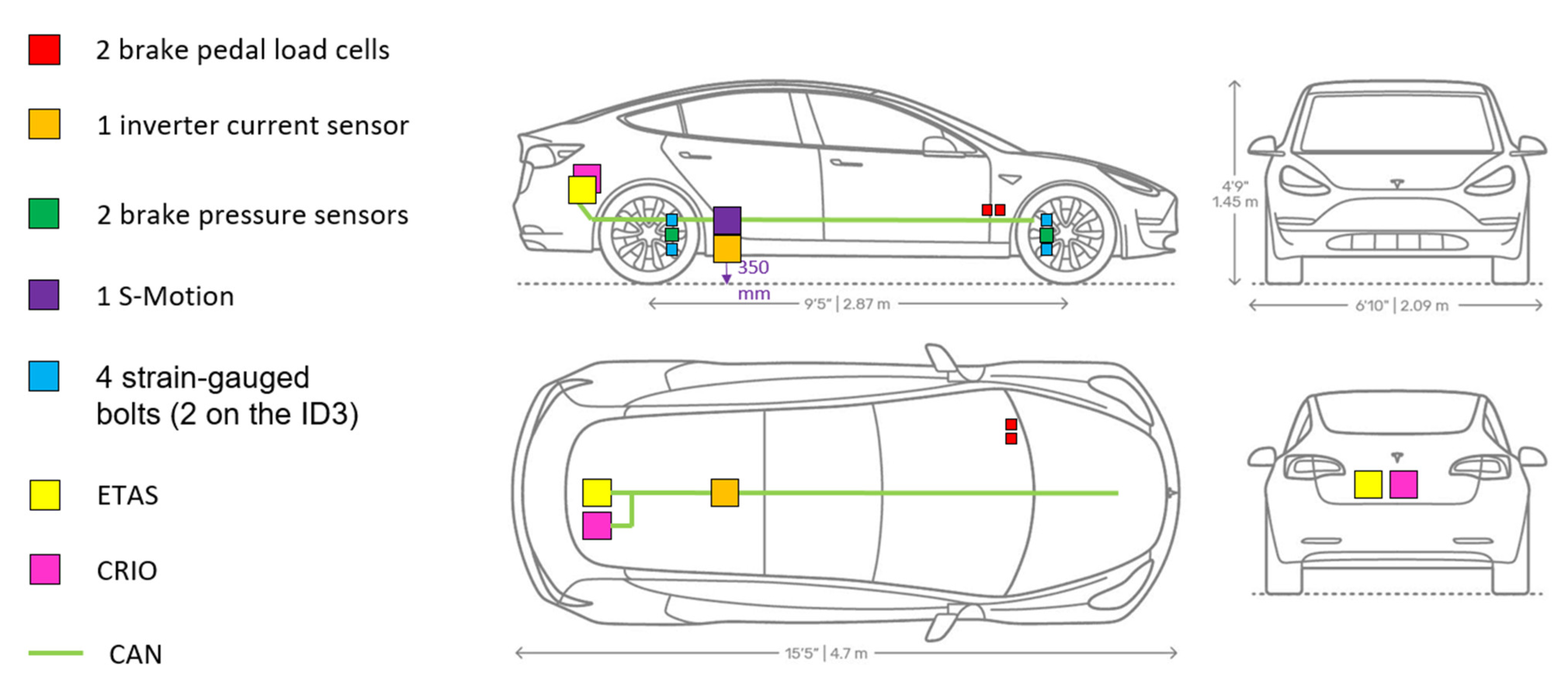
4.2. Experimental Methodology
- Body accelerations in the three directions;
- Vehicle speed;
- Pitch and roll angles and velocities;
- Yaw rate;
- Steering wheel angle and speed;
- Wheel rotational speed (FL, FR, RL, RR);
- Bus high voltage (front and rear);
- Bus current (front and rear);
- Acceleration pedal position;
- Brake pedal activation signal (ON/OFF);
- ABS activation flag;
- ESP activation flag and related parameters;
- Motor torque request (front and rear);
- Motor output torque (front and rear);
- Motor output power (front and rear);
- Envelope of motor phase current (front and rear);
- Battery state of charge;
- Battery voltage;
- GPS positioning (latitude and longitude).
- Validation—verification of each signal to guarantee the coherence and magnitude regarding the physical value anticipated;
- Data cleanse—cancelling of missing data points, zero values and other eventual outliers or faulty signals;
- Integration—gathering data from the different dataloggers, ensuring the synchronization of the information;
- Determination of the relevant maneuvers—the acquisition begins before the actual start of the maneuver, necessitating a “cut” of the data where useful information is lacking;
- Filtering—in signals with high noise, low-pass filters are applied to smooth the curve and help with the data analysis and comparison.
5. Experimental Results
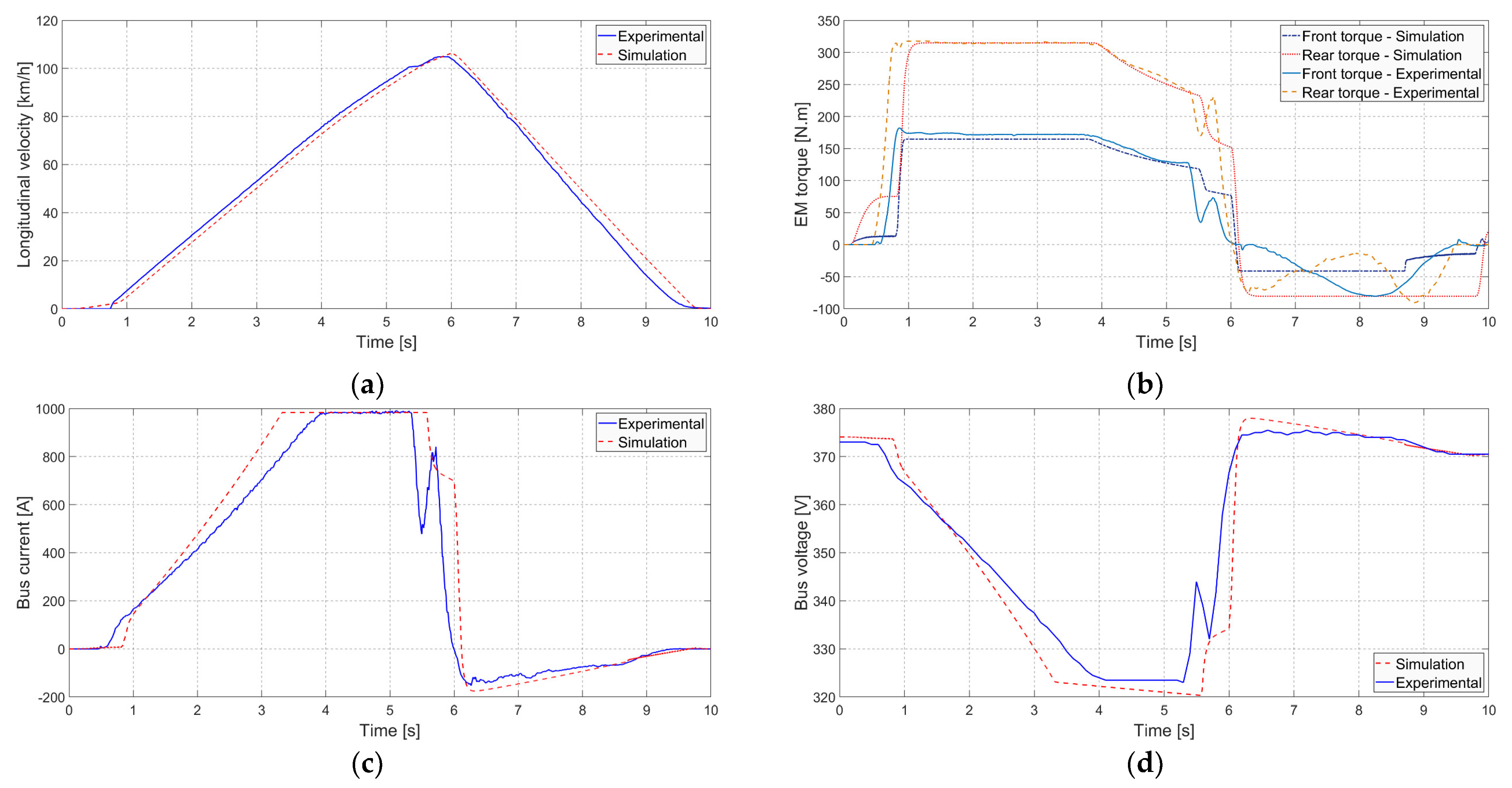
5.1. Straight Line 0-100-0 km/h
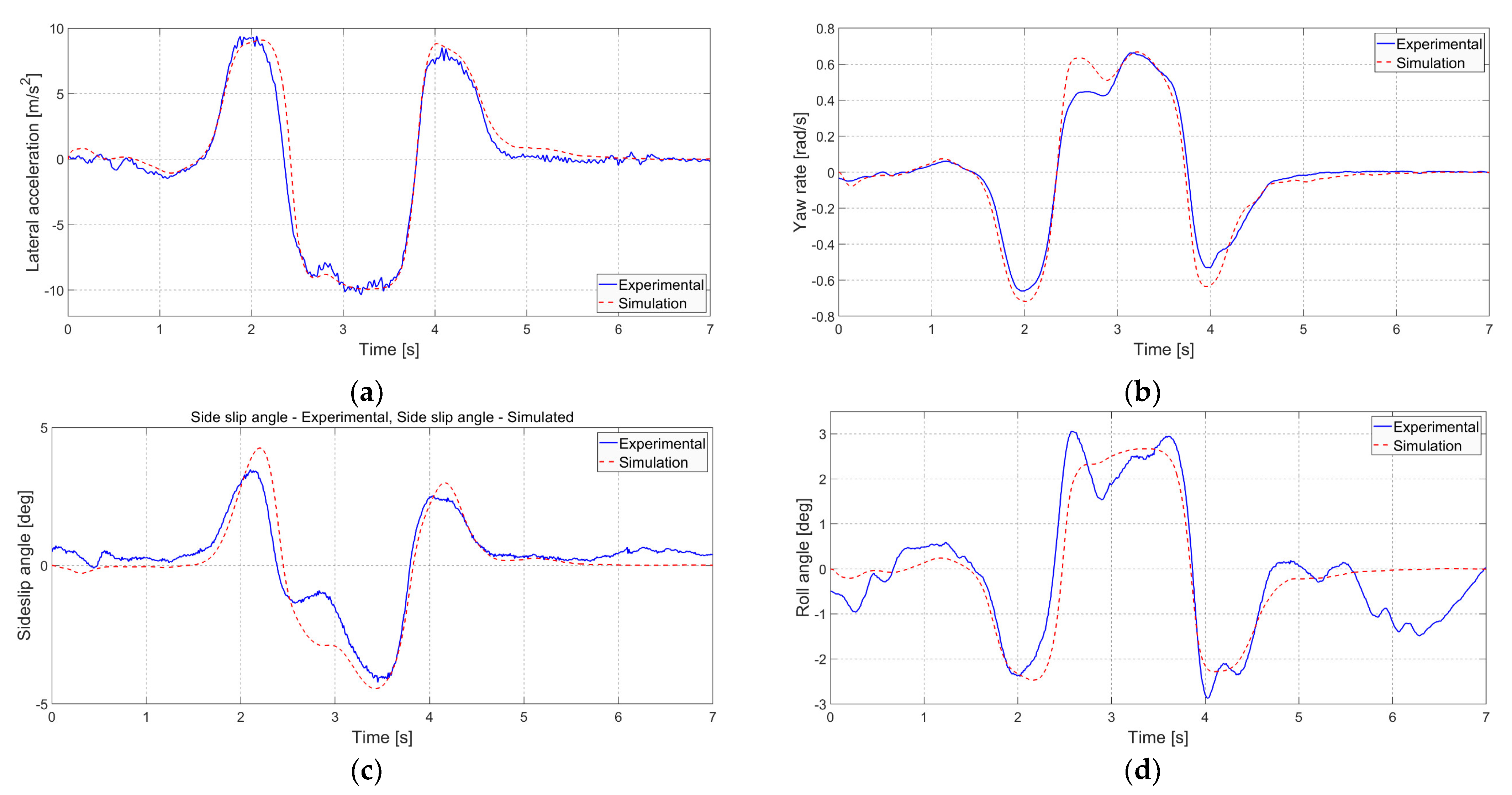
5.2. Double-Lane Change at 50 km/h
6. Conclusions
Funding
Data Availability Statement
Acknowledgments
Conflicts of Interest
References
- Automobile—Early Electric Automobiles|Britannica. March 2023. Available online: https://www.britannica.com/technology/automobile/Early-electric-automobiles (accessed on 29 November 2023).
- What Was the Henney Kilowatt? 2018. Available online: https://blog.consumerguide.com/what-was-the-henney-kilowatt/ (accessed on 29 November 2023).
- Shahan, Z. Electric Car History (In Depth). 2015. Available online: https://cleantechnica.com/2015/04/26/electric-car-history/ (accessed on 29 November 2023).
- Zero-Emission Vehicle Program|California Air Resources Board. March 2023. Available online: https://ww2.arb.ca.gov/our-work/programs/zero-emission-vehicle-program/about (accessed on 29 November 2023).
- Berdichevsky, G.; Kelty, K.; Straubel, J.; Toomre, E. The Tesla Roadster Battery System; Tesla Motors: Austin, TX, USA, 2006. [Google Scholar]
- Blomgren, G.E. The Development and Future of Lithium Ion Batteries. J. Electrochem. Soc. 2016, 164, A5019. [Google Scholar] [CrossRef]
- EEC. Council Directive 91/441/EEC of 26 June 1991 amending Directive 70/220/EEC on the approximation of the laws of the Member States relating to measures to be taken against air pollution by emissions from motor vehicles. Off. J. L 1991, 242, 1–106. [Google Scholar]
- Q&A: Commission Proposal on the New Euro 7 Standards, Text. March 2023. Available online: https://ec.europa.eu/commission/presscorner/detail/en/qanda_22_6496 (accessed on 29 November 2023).
- Fit for 55: Zero CO2 Emissions for New Cars and Vans in 2035|News|European Parliament. 2023. Available online: https://www.europarl.europa.eu/news/en/press-room/20230210IPR74715/fit-for-55-zero-co2-emissions-for-new-cars-and-vans-in-2035 (accessed on 29 November 2023).
- Deal Confirms Zero-Emissions Target for New Cars and Vans in 2035|News|European Parliament. 2022. Available online: https://www.europarl.europa.eu/news/en/press-room/20221024IPR45734/deal-confirms-zero-emissions-target-for-new-cars-and-vans-in-2035 (accessed on 29 November 2023).
- Frith, J.T.; Lacey, M.J.; Ulissi, U. A non-academic perspective on the future of lithium-based batteries. Nat. Commun. 2023, 14, 420. [Google Scholar] [CrossRef]
- Electric Vehicles—Worldwide|Statista Market Forecast. March 2023. Available online: https://www.statista.com/outlook/mmo/electric-vehicles/worldwide (accessed on 29 November 2023).
- Electric Vehicle Market Share, Size, Analysis|EV Market Growth. March 2023. Available online: https://www.alliedmarketresearch.com/electric-vehicle-market (accessed on 29 November 2023).
- Battery Recycling Policies for Boosting Electric Vehicle Adoption: Evidence from a Choice Experimental Survey. March 2023. Available online: https://www.springerprofessional.de/en/battery-recycling-policies-for-boosting-electric-vehicle-adoptio/23137392 (accessed on 29 November 2023).
- Nong, G.P.; Pang, S.L. Research on the Electric Vehicle Remanufacturable Battery Supply Chain with Recycling Channels. Adv. Mater. Res. 2013, 773, 948–953. [Google Scholar] [CrossRef]
- Feng, S. System dynamics model for battery recycling of electric vehicles in Anylogic simulation. Int. J. Internet Manuf. Serv. 2018, 5, 405–418. [Google Scholar] [CrossRef]
- Hao, F.; Lu, X.; Qiao, Y.; Chen, X. Crashworthiness Analysis of Electric Vehicle with Energy-Absorbing Battery Modules. J. Eng. Mater. Technol. 2017, 139, 021022. [Google Scholar] [CrossRef]
- Kang, S.; Kwon, M.; Yoon Choi, J.; Choi, S. Full-scale fire testing of battery electric vehicles. Appl. Energy 2023, 332, 120497. [Google Scholar] [CrossRef]
- Kim, S.; Lee, J.; Lee, C. Does Driving Range of Electric Vehicles Influence Electric Vehicle Adoption? Sustainability 2017, 9, 1783. [Google Scholar] [CrossRef]
- Kumar, L.; Ravi, N. Electric vehicle charging method and impact of charging and discharging on distribution system: A review. Int. J. Electr. Hybrid Veh. 2022, 14, 87–111. [Google Scholar] [CrossRef]
- Dong, J.; Lin, Z. Within-day recharge of plug-in hybrid electric vehicles: Energy impact of public charging infrastructure. Transp. Res. Part Transp. Environ. 2012, 17, 405–412. [Google Scholar] [CrossRef]
- Gruber, P.W.; Medina, P.A.; Keoleian, G.A.; Kesler, S.E.; Everson, M.P.; Wallington, T.J. Global Lithium Availability. J. Ind. Ecol. 2011, 15, 760–775. [Google Scholar] [CrossRef]
- Ahmed, S.; Nelson, P.A.; Gallagher, K.G.; Susarla, N.; Dees, D.W. Cost and energy demand of producing nickel manganese cobalt cathode material for lithium ion batteries. J. Power Sources 2017, 342, 733–740. [Google Scholar] [CrossRef]
- Rieck, F.; Machielse, K.; van Duin, R. Will Automotive Be the Future of Mobility? Striving for Six Zeros. World Electr. Veh. J. 2020, 11, 10. [Google Scholar] [CrossRef]
- Girardi, P.; Gargiulo, A.; Brambilla, P.C. A comparative LCA of an electric vehicle and an internal combustion engine vehicle using the appropriate power mix: The Italian case study. Int. J. Life Cycle Assess. 2015, 20, 1127–1142. [Google Scholar] [CrossRef]
- Eshetu, G.G.; Zhang, H.; Judez, X.; Adenusi, H.; Armand, M.; Passerini, S.; Figgemeier, E. Production of high-energy Li-ion batteries comprising silicon-containing anodes and insertion-type cathodes. Nat. Commun. 2021, 12, 5459. [Google Scholar] [CrossRef]
- Varzi, A.; Raccichini, R.; Passerini, S.; Scrosati, B. Challenges and prospects of the role of solid electrolytes in the revitalization of lithium metal batteries. J. Mater. Chem. A 2016, 4, 17251–17259. [Google Scholar] [CrossRef]
- Braga, M.H.; Grundish, N.S.; Murchison, A.J.; Goodenough, J.B. Alternative strategy for a safe rechargeable battery. Energy Environ. Sci. 2017, 10, 331–336. [Google Scholar] [CrossRef]
- Rizzello, A.; Scavuzzo, S.; Ferraris, A.; Airale, A.G.; Carello, M. Temperature-Dependent Thévenin Model of a Li-Ion Battery for Automotive Management and Control. In Proceedings of the 2020 IEEE International Conference on Environment and Electrical Engineering and 2020 IEEE Industrial and Commercial Power Systems Europe (EEEIC/I&CPS Europe), Madrid, Spain, 9–12 June 2020; IEEE: Madrid, Spain, 2020; pp. 1–6, ISBN 978-1-72817-455-6. [Google Scholar] [CrossRef]
- Rizzello, A.; Scavuzzo, S.; Ferraris, A.; Airale, A.G.; Bianco, E.; Carello, M. Non-linear Kalman Filters for Battery State of Charge Estimation and Control. In Proceedings of the 2021 International Conference on Electrical, Computer, Communications and Mechatronics Engineering (ICECCME), Piscataway, NJ, USA, 7–8 October 2021; pp. 1–7. [Google Scholar] [CrossRef]
- Christensen, J.; Albertus, P.; Sanchez-Carrera, R.S.; Lohmann, T.; Kozinsky, B.; Liedtke, R.; Ahmed, J.; Kojic, A. A Critical Review of Li/Air Batteries. J. Electrochem. Soc. 2011, 159, R1–R30. [Google Scholar] [CrossRef]
- Wang, H.; Yang, Y.; Liang, Y.; Robinson, J.T.; Li, Y.; Jackson, A.; Cui, Y.; Dai, H. Graphene-Wrapped Sulfur Particles as a Rechargeable Lithium–Sulfur Battery Cathode Material with High Capacity and Cycling Stability. Nano Lett. 2011, 11, 2644–2647. [Google Scholar] [CrossRef]
- Ji, X.; Lee, K.T.; Nazar, L.F. A highly ordered nanostructured carbon–sulphur cathode for lithium–sulphur batteries. Nat. Mater. 2009, 8, 500–506. [Google Scholar] [CrossRef]
- Hartmann, P.; Bender, C.L.; Sann, J.; Dürr, A.K.; Jansen, M.; Janek, J.; Adelhelm, P. A comprehensive study on the cell chemistry of the sodium superoxide (NaO2) battery. Phys. Chem. Chem. Phys. 2013, 15, 11661–11672. [Google Scholar] [CrossRef]
- Hartmann, P.; Bender, C.L.; Vračar, M.; Dürr, A.K.; Garsuch, A.; Janek, J.; Adelhelm, P. A rechargeable room-temperature sodium superoxide (NaO2) battery. Nat. Mater. 2013, 12, 228–232. [Google Scholar] [CrossRef] [PubMed]
- All-Solid-State Lithium-Ion Batteries. March 2023. Available online: https://www.hitachizosen.co.jp/english/business/field/functional/as-lib.html (accessed on 29 November 2023).
- Duan, Y.; Bai, X.; Yu, T.; Rong, Y.; Wu, Y.; Wang, X.; Yang, J.; Wang, J. Research progress and prospect in typical sulfide solid-state electrolytes. J. Energy Storage 2022, 55, 105382. [Google Scholar] [CrossRef]
- Suzuki, N.; Watanabe, T.; Fujiki, S.; Aihara, Y. Solid-State Batteries with Inorganic Electrolytes. In Encyclopedia of Electrochemistry; John Wiley & Sons, Ltd.: Hoboken, NJ, USA, 2020; pp. 1–62. ISBN 978-3-527-61042-6. [Google Scholar] [CrossRef]
- Carello, M.; Pinheiro, H.D.C.; Longega, L.; Di Napoli, L. Design and Modelling of the Powertrain of a Hybrid Fuel Cell Electric Vehicle. SAE Int. J. Adv. Curr. Pract. Mobil. 2021, 3, 2878–2892. [Google Scholar] [CrossRef]
- Bianco, E.; Di Napoli, L.; Grano, E.; Carello, M. E-scooter Modelling: Battery and Fuel Cell System Integration. In Advances in Italian Mechanism Science; Niola, V., Gasparetto, A., Quaglia, G., Carbone, G., Eds.; Springer International Publishing: Cham, Switzerland, 2022; pp. 909–916. ISBN 978-3-031-10776-4. [Google Scholar] [CrossRef]
- Bianco, E.; Carello, M. A first e-scooter powertrain analysis for Fuel Cell integration. In Proceedings of the 2022 International Conference on Electrical, Computer, Communications and Mechatronics Engineering (ICECCME), Maldives, Maldives, 16–18 November 2022; pp. 1–6. [Google Scholar] [CrossRef]
- Messana, A.; Airale, A.G.; Ferraris, A.; Sisca, L.; Carello, M. Correlation between thermo-mechanical properties and chemical composition of aged thermoplastic and thermosetting fiber reinforced plastic materials: Korrelation zwischen thermomechanischen Eigenschaften und chemischer Zusammensetzung von gealterten thermo- und duroplastischen faserverstärkten Kunst. Mater. Werkst. 2017, 48, 447–455. [Google Scholar] [CrossRef]
- Messana, A.; Sisca, L.; Ferraris, A.; Airale, A.G.; Pinheiro, H.d.C.; Sanfilippo, P.; Carello, M. From Design to Manufacture of a Carbon Fiber Monocoque for a Three-Wheeler Vehicle Prototype. Materials 2019, 12, 332. [Google Scholar] [CrossRef]
- Airale, A.; Carello, M.; Ferraris, A.; Sisca, L. Moisture effect on mechanical properties of polymeric composite materials. AIP Conf. Proc. 2016, 1736, 020020. [Google Scholar] [CrossRef]
- Carello, M.; Airale, A.G.; Ferraris, A.; Messana, A.; Sisca, L. Static Design and Finite Element Analysis of Innovative CFRP Transverse Leaf Spring. Appl. Compos. Mater. 2017, 24, 1493–1508. [Google Scholar] [CrossRef]
- Sisca, L.; Locatelli Quacchia, P.T.; Messana, A.; Airale, A.G.; Ferraris, A.; Carello, M.; Monti, M.; Palenzona, M.; Romeo, A.; Liebold, C.; et al. Validation of a Simulation Methodology for Thermoplastic and Thermosetting Composite Materials Considering the Effect of Forming Process on the Structural Performance. Polymers 2020, 12, 2801. [Google Scholar] [CrossRef]
- Carello, M.; Pinheiro, H.d.C.; Messana, A.; Freedman, A.; Ferraris, A.; Airale, A.G. Composite Control Arm Design: A Comprehensive Workflow. SAE Int. J. Adv. Curr. Pract. Mobil. 2021, 3, 2355–2369. [Google Scholar] [CrossRef]
- Fasana, A.; Ferraris, A.; Airale, A.G.; Berti Polato, D.; Carello, M. Experimental Characterization of Damped CFRP Materials with an Application to a Lightweight Car Door. Shock Vib. 2017, 2017, 7129058. [Google Scholar] [CrossRef]
- Carello, M.; Airale, A.G. Composite Suspension Arm Optimization for the City Vehicle XAM 2.0. In Design and Computation of Modern Engineering Materials; Öchsner, A., Altenbach, H., Eds.; Springer International Publishing: Cham, Switzerland, 2014; pp. 257–272. ISBN 978-3-319-07382-8. [Google Scholar] [CrossRef]
- Cubito, C.; Rolando, L.; Ferraris, A.; Carello, M.; Millo, F. Design of the Control Strategy for a Range Extended Hybrid Vehicle by means of Dynamic Programming Optimization. In Proceedings of the 2017 IEEE Intelligent Vehicles Symposium (IV), Los Angeles, USA, 11–14 June 2017; pp. 1234–1241. [Google Scholar] [CrossRef]
- Ferraris, A.; De Cupis, D.; De Carvalho Pinheiro, H.; Messana, A.; Sisca, L.; Airale, A.G.; Carello, M. Integrated Design and Control of Active Aerodynamic Features for High Performance Electric Vehicles; SAE Technical Paper 2020-36-0079; SAE International: Warrendale, PA, USA, 2021. [Google Scholar] [CrossRef]
- Brusaglino, G.; Buja, G.; Carello, M.; Carlucci, A.P.; Onder, C.H.; Razzetti, M. New technologies demonstrated at Formula Electric and Hybrid Italy 2008. World Electr. Veh. J. 2009, 3, 160–171. [Google Scholar] [CrossRef]
- Liu, B.; Zhang, H.; Zhu, S. An Incremental V-Model Process for Automotive Development. In Proceedings of the 2016 23rd Asia-Pacific Software Engineering Conference (APSEC), Hamilton, New Zealand, 6–9 December 2016; pp. 225–232. [Google Scholar] [CrossRef]
- Castellanos Molina, L.M.; Manca, R.; Hegde, S.; Amati, N.; Tonoli, A. Predictive handling limits monitoring and agility improvement with torque vectoring on a rear in-wheel drive electric vehicle. Veh. Syst. Dyn. 2023, 1–25. [Google Scholar] [CrossRef]
- Pinheiro, H.d.C.; Punta, E.; Carello, M.; Ferraris, A.; Airale, A.G. Torque Vectoring in Hybrid Vehicles with In-Wheel Electric Motors: Comparing SMC and PID control. In Proceedings of the 2021 IEEE International Conference on Environment and Electrical Engineering and 2021 IEEE Industrial and Commercial Power Systems Europe (EEEIC/I CPS Europe), Bari, Italy, 7–10 September 2021; pp. 1–6. [Google Scholar] [CrossRef]
- Tramacere, E.; Castellanos, L.M.M.; Amati, N.; Tonoli, A.; Bonfitto, A. Adaptive LQR Control for a Rear-Wheel Steering Battery Electric Vehicle. In Proceedings of the 2022 IEEE Vehicle Power and Propulsion Conference (VPPC), Merced, CA, USA, 1–4 November 2022; pp. 1–6. [Google Scholar] [CrossRef]
- De Carvalho Pinheiro, H.; Carello, M. Design and Validation of a High-Level Controller for Automotive Active Systems. SAE Int. J. Veh. Dyn. Stab. NVH 2023, 7, 83–98. [Google Scholar] [CrossRef]
- Vošahlík, D.; Haniš, T. Traction Control Allocation Employing Vehicle Motion Feedback Controller for Four-Wheel-Independent-Drive Vehicle. IEEE Trans. Intell. Transp. Syst. 2023, 24, 14570–14579. [Google Scholar] [CrossRef]
- Carello, M.; Ferraris, A.; Pinheiro, H.d.C.; Stanke, D.C.; Gabiati, G.; Camuffo, I.; Grillo, M. Human-Driving Highway Overtake and Its Perceived Comfort: Correlational Study Using Data Fusion. In Proceedings of the WCX SAE World Congress Experience, Detroit, MI, USA, 21–23 April 2020. SAE Technical Paper 2020-01-1036. [Google Scholar] [CrossRef]
- Pinheiro, H.d.C.; Stanke, D.C.; Ferraris, A.; Carello, M.; Gabiati, G.; Camuffo, I.; Grillo, M. Autonomous Driving Scenario Generation in Overtake Manoeuvres Through Data Fusion. In Advances in Italian Mechanism Science; Niola, V., Gasparetto, A., Eds.; Springer: Berlin/Heidelberg, Germany, 2021; pp. 786–794. ISBN 978-3-030-55807-9. [Google Scholar] [CrossRef]
- Milliken, W.F. Race Car Vehicle Dynamics; Society of Automotive Engineers: Warrendale, PA, USA, 1995; ISBN 978-0-7680-0103-7. [Google Scholar]
- Pinheiro, H.d.C.; Carello, M.; Punta, E. Torque Vectoring Control Strategies Comparison for Hybrid Vehicles with Two Rear Electric Motors. Appl. Sci. 2023, 13, 8109. [Google Scholar] [CrossRef]
- Genta, G.; Morello, L. The Automotive Chassis; Springer Science & Business Media: Berlin/Heidelberg, Germany, 2008; Volume 1–2, ISBN 978-1-4020-8676-2. [Google Scholar]
- VI-grade GmbH. VI-CarRealTime 20.0 Documentation; VI-grade GmbH: Darmstadt, Germany, 2020. [Google Scholar]
- Ydrefors, L.; Hjort, M.; Kharrazi, S.; Jerrelind, J.; Stensson Trigell, A. Rolling resistance and its relation to operating conditions: A literature review. Proc. Inst. Mech. Eng. Part J. Automob. Eng. 2021, 235, 2931–2948. [Google Scholar] [CrossRef]
- Nicoletti, L.; Mayer, S.; Brönner, M.; Schockenhoff, F.; Lienkamp, M. Design Parameters for the Early Development Phase of Battery Electric Vehicles. World Electr. Veh. J. 2020, 11, 47. [Google Scholar] [CrossRef]
- Electric Powertrain: Energy Systems, Power Electronics and Drives for Hybrid, Electric and Fuel Cell Vehicles | Wiley. April 2023. Available online: https://www.wiley.com/en-au/Electric+Powertrain%3A+Energy+Systems%2C+Power+Electronics+and+Drives+for+Hybrid%2C+Electric+and+Fuel+Cell+Vehicles-p-9781119063643 (accessed on 29 November 2023).
- Krishnan, R. Electric Motor Drives: Modeling, Analysis, and Control; Pearson: London, UK, 2001; ISBN 978-0-13-091014-1. [Google Scholar]
- Bianco, E.; Rizzello, A.; Ferraris, A.; Carello, M. Modeling and experimental validation of vehicle’s electric powertrain. In Proceedings of the 2022 IEEE International Conference on Environment and Electrical Engineering and 2022 IEEE Industrial and Commercial Power Systems Europe (EEEIC /I&CPS Europe), Prague, Czech Republic, 28 June–1 July 2022; pp. 1–6. [Google Scholar] [CrossRef]
- Grano, E.; Bianco, E.; De Carvalho Pinheiro, H.; Carello, M. MTPA and flux weakening control of electric motors: A numerical approach. In Proceedings of the 2023 IEEE International Conference on Environment and Electrical Engineering and 2023 IEEE Industrial and Commercial Power Systems Europe (EEEIC/I&CPS Europe), Madrid, Spain, 6–9 June 2023; pp. 1–7. [Google Scholar] [CrossRef]
- Muhlethaler, J.; Biela, J.; Kolar, J.W.; Ecklebe, A. Core Losses Under the DC Bias Condition Based on Steinmetz Parameters. IEEE Trans. Power Electron. 2012, 27, 953–963. [Google Scholar] [CrossRef]
- Ciampolini, M.; Fazzini, L.; Berzi, L.; Ferrara, G.; Pugi, L. Simplified Approach for Developing Efficiency Maps of High-Speed PMSM Machines for Use in EAT Systems Starting from Single-Point Data. In Proceedings of the 2020 IEEE International Conference on Environment and Electrical Engineering and 2020 IEEE Industrial and Commercial Power Systems Europe (EEEIC/I&CPS Europe), Madrid, Spain, 9–12 June 2020; pp. 1–6. [Google Scholar] [CrossRef]
- Stevens, J. Fundamentals of Thermal Resistance, HeatSink blog by Celsia. 2018. Available online: https://celsiainc.com/heat-sink-blog/fundamentals-of-thermal-resistance/ (accessed on 29 November 2023).
- Wang, B.; Nie, Y.; Yang, Z.; Zong, C.; Geng, L. Study on the Barycenter Position of Measurement and Data Processing for Dura-Axle Vehicle; Atlantis Press: Amsterdam, The Netherlands, 2016; ISBN 978-94-6252-188-9. [Google Scholar] [CrossRef]
- Zhao, X.; Kang, J.; Lei, T.; Wang, Y.; Cao, Z. Vehicle Centroid Measurement System Based On Forward Tilt Method Error Analysis. IOP Conf. Ser. Mater. Sci. Eng. 2018, 452, 042189. [Google Scholar] [CrossRef]
- Pinheiro, H.d.C.; Messana, A.; Carello, M.; Rosso, N. Multibody Parameter Estimation: A Comprehensive Case-Study for an Innovative Rear Suspension. In Proceedings of the SAE BRASIL 2022 Congress, Sao Paulo, Brazil, 24–27 November 2022; SAE Technical Paper 2022-36-0059. SAE International: Sao Paulo, Brazil, 2023. [Google Scholar] [CrossRef]
- Fehér, Á.; Aradi, S.; Bécsi, T. Hierarchical Evasive Path Planning Using Reinforcement Learning and Model Predictive Control. IEEE Access 2020, 8, 187470–187482. [Google Scholar] [CrossRef]
- BS ISO 3888-2:2011; Passenger Cars—Test Track for a Severe Lane-Change Manoeuvre. ISO International Standards: Geneva, Switzerland, 2011.
- De Carvalho Pinheiro, H.; Sisca, L.; Carello, M.; Ferraris, A.; Airale, A.G.; Falossi, M.; Carlevaris, A. Methodology and Application on Load Monitoring Using Strain-Gauged Bolts in Brake Calipers; SAE Technical Paper 2022-01-0922; SAE International: Warrendale, PA, USA, 2022. [Google Scholar] [CrossRef]


| Parameter | Value | Unit |
|---|---|---|
| wheelbase | 2875 | mm |
| track | 1580 | mm |
| mass LF | 517 | kg |
| mass RF | 505 | kg |
| mass LR | 530 | kg |
| mass RR | 518 | kg |
| total mass | 2070 | kg |
| unsprung mass front | 22.7 | kg |
| unsprung mass rear | 19.5 | kg |
| sprung mass | 1985.6 | kg |
| CoG x | 1419 | mm |
| CoG y | 18 | mm |
| CoG z | 468 | mm |
| Ixx | 2.65 × 10⁸ | kg × mm2 |
| Iyy | 1.04 × 10⁹ | kg × mm2 |
| Izz | 1.69 × 10⁹ | kg × mm2 |
| Ixy | 3.22 × 10⁶ | kg × mm2 |
| Ixz | 4.14 × 10⁷ | kg × mm2 |
| Iyz | 4.15 × 10⁵ | kg × mm2 |
| Parameter | Value | Unit |
|---|---|---|
| Air density | 1.225 | kg/m3 |
| Frontal area | 2.22 | m2 |
| Drag coefficient (Cx) | 0.23 | - |
| Lift coefficient (Cz) | 0.09 | - |
| CoP distribution | 0.5 | - |
| Parameter | Value | Unit |
|---|---|---|
| Cell height | 70 | mm |
| Cell diameter | 21 | mm |
| Cell mass | 68.5 | g |
| Nominal capacity | 4.80 | Ah |
| Maximum continuous current | 7.0 | A |
| Maximum peak current | 17.8 | A |
| Energy @ C/10 | 17.1 | Wh |
| Continuous power | 24.0 | W |
| Peak power | 64.6 | W |
| SOC | VOC [V] | ] | ] | ] | ] | ] |
|---|---|---|---|---|---|---|
| 0.00 | 2.75 | 0.030 | 0.0064 | 200 | 0.0064 | 1000 |
| 0.10 | 2.96 | 0.028 | 0.0064 | 250 | 0.0064 | 2500 |
| 0.20 | 3.17 | 0.026 | 0.0072 | 750 | 0.0064 | 8500 |
| 0.30 | 3.33 | 0.027 | 0.0072 | 1100 | 0.0064 | 12,000 |
| 0.40 | 3.53 | 0.025 | 0.0072 | 1450 | 0.0064 | 10,000 |
| 0.50 | 3.72 | 0.023 | 0.008 | 1650 | 0.008 | 15,000 |
| 0.60 | 3.88 | 0.024 | 0.0088 | 1800 | 0.0096 | 21,500 |
| 0.70 | 3.96 | 0.026 | 0.0088 | 2000 | 0.008 | 15,000 |
| 0.80 | 4.08 | 0.027 | 0.0128 | 2250 | 0.0096 | 15,000 |
| 0.90 | 4.18 | 0.029 | 0.024 | 2100 | 0.016 | 22,500 |
| 1.00 | 4.20 | 0.030 | 0.0216 | 2250 | 0.02 | 30,000 |
| Parameter | Value | Unit |
|---|---|---|
| Front motor (Induction Motor) | ||
| Pole pairs | 2 | - |
| Max continuous current | 532 | A |
| Max peak current | 940 | A |
| Max continuous torque | 172 | N × m |
| Max peak torque | 220 | N × m |
| Max continuous power | 89.77 | kW |
| Max peak power | 158.0 | kW |
| Max rotational speed | 18,000 | rpm |
| Rotational inertia | 0.1 | kg × m2 |
| Transmission ratio | 9:1 | - |
| Rear motor (Synchronous Motor) | ||
| Pole pairs | 3 | - |
| Max continuous current | 600 | A |
| Max peak current | 1000 | A |
| Max continuous torque | 315 | N × m |
| Max peak torque | 430 | N × m |
| Max continuous power | 110.0 | kW |
| Max peak power | 192.0 | kW |
| Max rotational speed | 18,000 | rpm |
| Rotational inertia | 0.1 | kg × mm2 |
| Transmission ratio | 9:1 | - |
Disclaimer/Publisher’s Note: The statements, opinions and data contained in all publications are solely those of the individual author(s) and contributor(s) and not of MDPI and/or the editor(s). MDPI and/or the editor(s) disclaim responsibility for any injury to people or property resulting from any ideas, methods, instructions or products referred to in the content. |
© 2023 by the author. Licensee MDPI, Basel, Switzerland. This article is an open access article distributed under the terms and conditions of the Creative Commons Attribution (CC BY) license (https://creativecommons.org/licenses/by/4.0/).
Share and Cite
de Carvalho Pinheiro, H. PerfECT Design Tool: Electric Vehicle Modelling and Experimental Validation. World Electr. Veh. J. 2023, 14, 337. https://doi.org/10.3390/wevj14120337
de Carvalho Pinheiro H. PerfECT Design Tool: Electric Vehicle Modelling and Experimental Validation. World Electric Vehicle Journal. 2023; 14(12):337. https://doi.org/10.3390/wevj14120337
Chicago/Turabian Stylede Carvalho Pinheiro, Henrique. 2023. "PerfECT Design Tool: Electric Vehicle Modelling and Experimental Validation" World Electric Vehicle Journal 14, no. 12: 337. https://doi.org/10.3390/wevj14120337