Article

Intelligent Resource Orchestration for 5G Edge Infrastructures

by
Rafael Moreno-Vozmediano
1,*,†,
Rubén S. Montero
1,2,†,
Eduardo Huedo
1,† and
Ignacio M. Llorente
2,†
1
Faculty of Computer Science, Complutense University of Madrid, 28040 Madrid, Spain
2
OpenNebula Systems, Paseo del Club Deportivo 1, Pozuelo de Alarcón, 28223 Madrid, Spain
*
Author to whom correspondence should be addressed.
These authors contributed equally to this work.
Future Internet 2024, 16(3), 103; https://doi.org/10.3390/fi16030103
Submission received: 16 February 2024 / Revised: 11 March 2024 / Accepted: 16 March 2024 / Published: 19 March 2024
(This article belongs to the Special Issue Edge Intelligence: Edge Computing for 5G and the Internet of Things)

Abstract

:
The adoption of edge infrastructure in 5G environments stands out as a transformative technology aimed at meeting the increasing demands of latency-sensitive and data-intensive applications. This research paper presents a comprehensive study on the intelligent orchestration of 5G edge computing infrastructures. The proposed Smart 5G Edge-Cloud Management Architecture, built upon an OpenNebula foundation, incorporates a ONEedge5G experimental component, which offers intelligent workload forecasting and infrastructure orchestration and automation capabilities, for optimal allocation of virtual resources across diverse edge locations. The research evaluated different forecasting models, based both on traditional statistical techniques and machine learning techniques, comparing their accuracy in CPU usage prediction for a dataset of virtual machines (VMs). Additionally, an integer linear programming formulation was proposed to solve the optimization problem of mapping VMs to physical servers in distributed edge infrastructure. Different optimization criteria such as minimizing server usage, load balancing, and reducing latency violations were considered, along with mapping constraints. Comprehensive tests and experiments were conducted to evaluate the efficacy of the proposed architecture.

1. Introduction

The evolution of 5G technology has ushered in a new era of connectivity, offering enhanced capabilities that extend beyond traditional communication paradigms. Advanced 5G networks facilitate a diverse range of applications, characterized by their complexity, computational demand, and low-latency requirements. These applications, designed to leverage the capabilities of advanced 5G, exhibit a hybrid profile, relying on resources spanning the spectrum from data centers to the cloud to the edge.
In particular, the deployment of edge infrastructure in 5G environments is crucial to addressing the unique challenges posed by latency-sensitive and data-intensive applications [1,2]. The next generation of applications, encompassing smart IoT applications, real-time analytics, machine learning applications, and more, require intelligent orchestration of resources in the edge domain, where computational tasks are strategically placed closer to data sources to minimize latency and enhance overall system performance.
Orchestrating edge infrastructure in 5G environments is not without its complexities. The heterogeneous nature of edge devices, coupled with the dynamic and resource-constrained characteristics of these environments, presents challenges for effective resource management. Unlike traditional cloud-centric models, the edge requires a nuanced approach that considers factors such as reliability, security, data protection, and energy efficiency. In light of these challenges, the need for intelligent orchestration becomes paramount. An orchestration system driven by artificial intelligence (AI) and machine learning (ML) techniques can dynamically allocate and coordinate resources across a distributed edge infrastructure.
In the current cloud market, various vendors and tools claim to employ intelligent techniques for resource management and monitoring. For instance, VMware implements a predictive distributed resource scheduler (DRS) [3] for cloud platforms, which forecasts future demand and preemptively addresses potential hot spots, by reallocating workloads well in advance of any contention. OPNI [4], an open source project from SUSE, is another noteworthy example aimed at enhancing observability, monitoring, and logging in Kubernetes-based clusters. It offers a range of AIOps tools for detecting log anomalies, identifying root causes, and spotting metric irregularities. Google Active Assist [5] is another tool that aims to provide intelligent solutions for improving cloud operations, by offering recommendations for cost reduction, performance enhancement, security improvement, and sustainability. Generally, these prediction and optimization techniques deployed by cloud stakeholders are tailored for centralized cloud platforms and often comprise simple, proprietary solutions that may not be adaptable to highly distributed 5G edge environments. On the other hand, recent initiatives like OpenNebula OneEdge [6] enable the deployment and management of geo-distributed edge/cloud infrastructures, leveraging resources from various public cloud and edge infrastructure providers. However, these tools are still nascent and primarily offer basic management functionalities rather than advanced, intelligent orchestration capabilities for optimizing the deployment of large scale edge infrastructures.
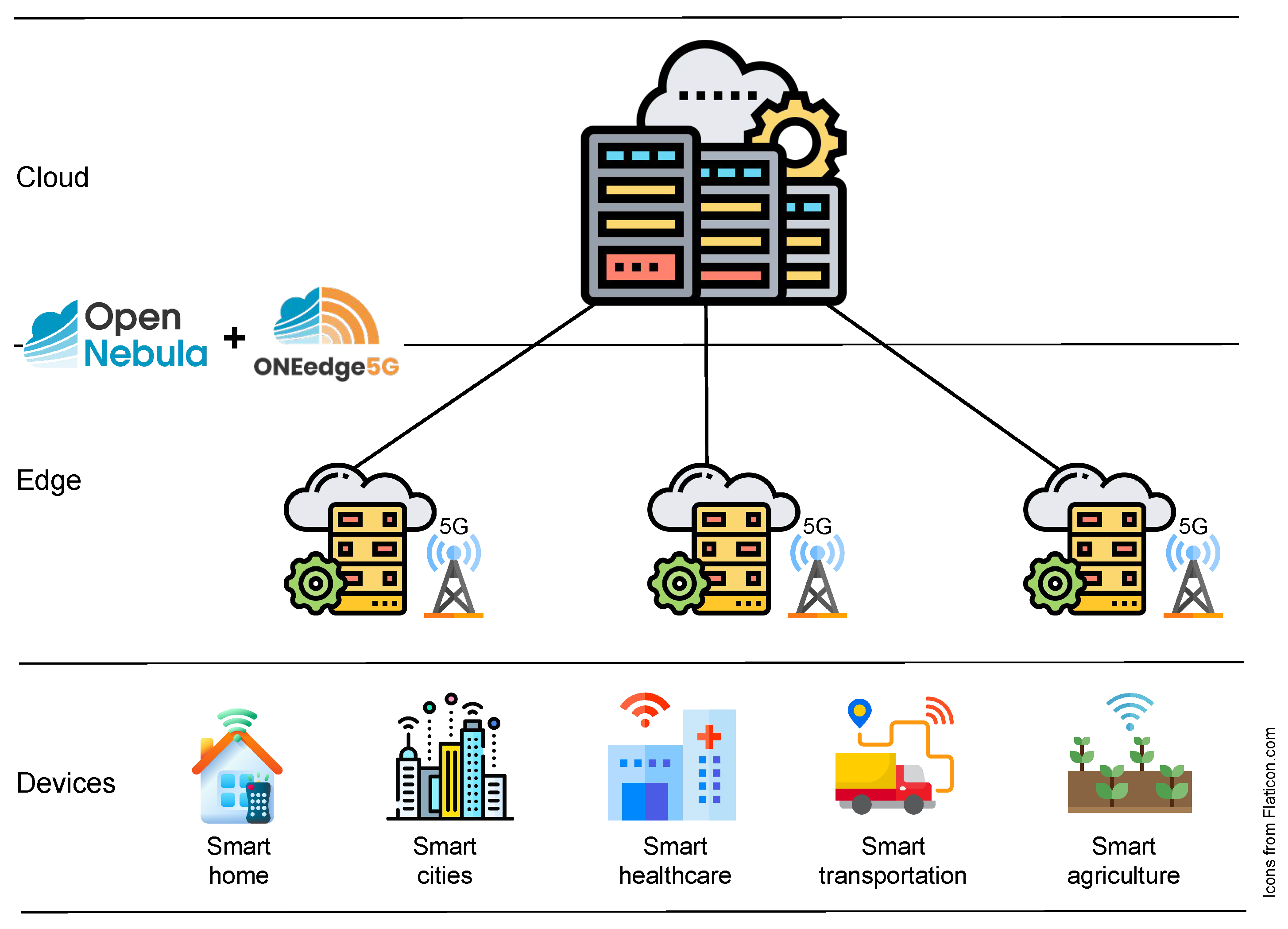
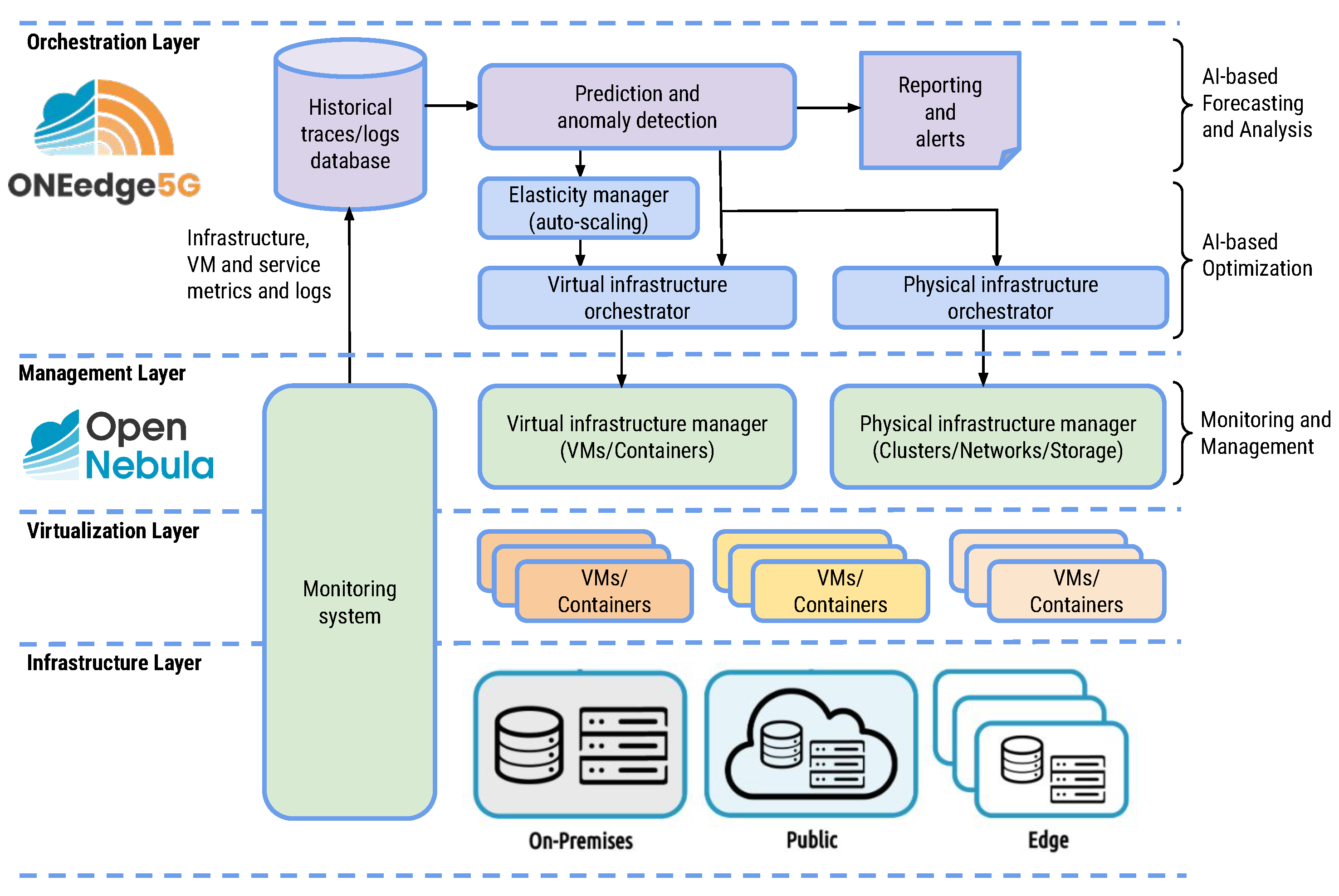
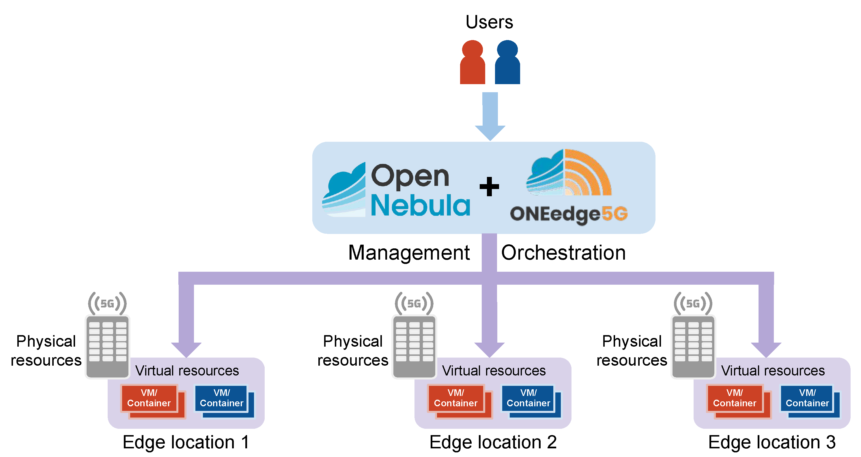
In this work, we propose a pioneering Smart 5G Edge-Cloud Management Architecture, which seeks to expand the existing edge management platforms by integrating intelligent orchestration capabilities. This integration aims to automate and optimize the provisioning and deployment of geographically distributed 5G edge infrastructures. This architecture, built upon the foundation of OpenNebula [7,8], will integrate cutting-edge experimental components under development in the ONEedge5G project, as shown in Figure 1. ONEedge5G aims to enable efficient capacity planning, provisioning, and risk prevention in geographically distributed edge infrastructures and applications within the context of advanced 5G networks. This is achieved through the characterization and monitoring of edge infrastructures and virtual applications, prediction of the state of the data center–cloud–edge continuum, and programmatic intervention based on these predictions.
In its current developmental phase, ONEedge5G integrates diverse predictive intelligence mechanisms for workload forecasting. It also embeds various optimization algorithms to ensure optimal resource allocation across multiple edge locations. This paper introduces and assesses these intelligent techniques, demonstrating their effectiveness for improving the management and performance of distributed edge infrastructures.
To evaluate the efficacy of our Smart 5G Edge-Cloud Management Architecture, we conducted comprehensive tests and experiments. Through rigorous analysis, we assessed the capabilities of a ONEedge5G prototype in accurate workload forecasting and optimization. By presenting the results of these experiments, we demonstrate the benefits and efficiency gains achieved by leveraging intelligent prediction and optimization techniques in 5G edge management.
The remainder of this paper is structured as follows: Section 2 analyzes the advantages and challenges of edge computing on 5G networks. Section 3 discusses related works. Section 4 presents the design and main components of the Smart 5G Edge-Cloud Management Architecture. Section 5 summarizes the time-series forecasting models employed for workload prediction. Section 6 introduces the mathematical models utilized in the integer linear programming (ILP) formulation for edge resource optimization. Section 7 demonstrates the virtual resource CPU usage forecasting results for the different datasets and the resource optimization outcomes for the various objective functions and constraints. Finally, Section 8 summarizes the conclusions of this study and suggests potential directions for future research.

2. Edge Computing and Advanced 5G Networks

Advanced 5G networks bring a multitude of advantages [9], including significantly faster data speeds, through enhanced mobile broadband (eMBB), ultra-reliable and low-latency communication (URLLC), and support for a large number of connected devices with massive machine-type communication (mMTC). The implementation of network slicing allows customizable network services, tailoring offerings to specific requirements, while technologies like beamforming and MIMO contribute to improved network coverage and efficiency. Deploying edge computing infrastructures on advanced 5G networks offers several key benefits. First, it significantly reduces latency by processing data closer to the source, ensuring quicker response times for applications. This is particularly crucial for real-time applications like augmented reality and autonomous vehicles. Second, edge computing enhances energy efficiency by minimizing data transmission between central clouds and end devices, contributing to a more sustainable network. Third, the proximity of computational resources at the edge ensures improved application performance, particularly for latency-sensitive tasks. The combination of these technologies, along with the growth of the Internet of Things (IoT), has given rise to the emergence of new computing paradigms, such as multi-access edge computing (MEC) [10], which is aimed at extending cloud computing capabilities to the edge of the radio access network, hence providing real-time, high-bandwidth, and low-latency access to radio network resources.
According to [11], the main objectives of edge computing in 5G environments are the following: (1) improving data management, in order to handle the large amounts of real-time delay-sensitive data generated by user equipments (UEs); (2) improving quality of service (QoS) to meet diverse QoS requirements, thereby improving the quality of experience (QoE) for applications that demand low latency and high bandwidth; (3) predicting network demand, which involves estimating the network resources required to cater to local proximity network (or user) demand, and subsequently providing optimal resource allocation; (4) managing location awareness, to enable geographically distributed edge servers to infer their own locations and track the location of UEs to support location-based services; and (5) improving resource management, in order to optimize network resource utilization for network performance enhancement in the edge cloud, acknowledging the challenges of catering to diverse applications, user requirements, and varying demands with limited resources compared to the central cloud.
Focusing on the last objective, efficient resource management and orchestration in 5G edge computing [12,13] are crucial as they not only contribute to latency reduction by strategically deploying computing resources, minimizing the time for data processing and enhancing application responsiveness, but also play a pivotal role in optimizing energy consumption through dynamic allocation based on demand, thereby reducing the environmental footprint. Furthermore, proper resource management is essential for performance optimization, preventing bottlenecks, ensuring balanced workload distribution, and maintaining consistent application performance, all of which collectively enhance the overall user experience in these advanced network environments. In this context, AI and ML techniques prove instrumental in addressing these challenges [14,15,16,17,18]. For example, through predictive analytics and forecasting, ML algorithms can anticipate future demands, enabling proactive resource allocation and strategic deployment for minimized data processing times and reduced latency. AI-driven dynamic allocation can optimize resource utilization and, consequently, energy consumption by adapting to real-time demand patterns. Additionally, ML models, employing clustering and anomaly detection, can ensure consistent application performance by preventing bottlenecks and optimizing workload distribution.
In this article, we specifically address the issue of intelligent resource orchestration in distributed edge computing infrastructures by integrating forecasting techniques for predicting resource utilization [19,20] and optimization techniques for optimal resource allocation [21,22]. Resource utilization forecasting leverages historical and real-time data to predict future resource demands accurately. By employing both traditional statistical techniques and AI-based ML techniques [23,24], these forecasts enable proactive resource allocation, mitigating the risk of resource shortages or over-provisioning. Furthermore, forecasting techniques facilitate capacity planning, allowing organizations to scale their resources dynamically based on anticipated demands. Optimization techniques also play a vital role in orchestrating resources across multiple edge locations. These techniques employ mathematical models such as ILP and heuristic algorithms [25,26] to determine the optimal mapping of virtual resources (VMs or containers) onto physical servers. By considering various factors including proximity, resource availability, and application requirements, these techniques ensure efficient utilization of resources and minimize resource fragmentation.

3. Related Work

The literature has extensively explored the application of artificial intelligence (AI) techniques, including evolutionary algorithms and machine learning (ML) algorithms, to address diverse prediction and optimization challenges in both cloud and edge environments. A recent study [27] offered a comprehensive review of machine-learning-based solutions for resource management in cloud computing. This review encompassed areas such as workload estimation, task scheduling, virtual machine (VM) consolidation, resource optimization, and energy efficiency techniques. Additionally, a recent book [28] compiled various research works that considered optimal resource allocation, energy efficiency, and predictive models in cloud computing. These works leveraged a range of ML techniques, including deep learning and neural networks. For edge computing platforms, surveys such as [29] have analyzed different machine and deep learning techniques for resource allocation in multi-access edge computing. Similarly, ref. [30] provided a review of task allocation and optimization techniques in edge computing, covering centralized, decentralized, hybrid, and machine learning algorithms.
If we focus on workload prediction, we see this is an essential technique in cloud computing environments, as it enables providers to effectively manage and allocate cloud resources, save on infrastructure costs, implement auto-scaling policies, and ensure compliance with service-level agreements (SLAs) with users. Workload prediction can be performed at application or infrastructure level. Application-level techniques [31,32] involve predicting a metric related to the application demand (e.g., requests per second or task arrival rate) to anticipate the optimal amount of resources needed to meet that demand. On the other hand, infrastructure-level techniques [33,34] are based on predicting one or more resource usage metrics (such as CPU, memory, disk, or network) and making advanced decisions about the optimal amount and size of virtual or physical resources to provision to avoid overload or over-sizing situations. Another interesting piece of research in this area is [35], which presented a taxonomy of the various real-world metrics used to evaluate the performance of cloud, fog, and edge computing environments.
The most common workload prediction techniques used in cloud computing are based on time-series prediction methods [19,24], which involve collecting historical data of the target metric (e.g., the historical CPU usage of a VM or group of VMs) and forecasting future values of that metric for a certain time horizon. There are many different methods for modeling and predicting the time-series used in cloud computing, many of them based on classical techniques such as linear regression [36], Bayesian models [37], or ARIMA statistical methods [38]. The main advantage of these models is their flexibility and simplicity in representing different types of time-series, making them quick and easy to use. However, they have a significant limitation in their linear behavior, making them inadequate in some practical situations.
More recently, different methods have been proposed for time-series prediction based on machine learning and deep learning models [34,39,40] using artificial neural networks that have inherent non-linear modeling capabilities. One of the most common ML models applied to time-series is the long short-term memory (LSTM) neural network [23,41,42], which overcomes the problem of vanishing gradients associated with other neural networks. However, these methods also have several drawbacks. The first is that the training and prediction times of the neural network can be quite high (several minutes, or even hours), making them unfeasible in certain situations. The second problem is that the quality of predictions of neural-network-based methods depends heavily on correct selection of the model’s hyperparameters, which can vary depending on the input data, meaning that adjusting these hyperparameters poses a serious challenge, even for expert analysts.
In absolute terms, it is not possible to claim that one prediction method is better than another, as their behavior will depend on the specific use case, the profile of the input data, the correct tuning of each model’s hyperparameters, and the use or non-use of co-variables that may correlate with the variable being predicted. In this context, research in this field involves exploring and comparing different prediction methods for each case, improving existing methods, and combining different techniques by proposing new hybrid or adaptive methods that allow for the most accurate forecasts possible. Likewise, applying these prediction techniques to other emerging environments such as highly geo-distributed edge/cloud environments, IoT environments, and server-less environments also represents a significant challenge.
On the other hand, the optimal allocation of resources in cloud computing is an important problem that must be addressed to ensure efficient use of resources and to meet SLAs agreed with users. The goal is to allocate resources (e.g., VMs to physical hosts) in a way that maximizes infrastructure utilization, subject to certain performance or application response time requirements.
There are different optimization techniques used to solve this problem. One of the most commonly used techniques is linear programming, which finds the optimal solution to a linear function subject to a set of linear constraints. This technique is very useful for problems involving a large number of variables and constraints. For example, ref. [43] was a pioneering work in cloud brokering that used ILP to optimize the cost of a virtual infrastructure deployed on a set of cloud providers. Subsequently, this research was expanded upon in [44], which addressed dynamic cloud scenarios and incorporated diverse optimization criteria such as cost or performance. The authors in [45,46] presented MALLOOVIA, a multi-application load-level-based optimization for virtual machine allocation. MALLOOVIA formulates an optimization problem based on ILP and takes the levels of performance to must be reached by a set of applications as input, and generates a VM allocation to support the performance requirements of all applications as output.The authors in [47,48] provided an approach for supporting the deployment of microservices in multi-cloud environments, focusing on the quality of monitoring and adopting a multi-objective mixed integer linear optimization problem, in order to find the optimal deployment satisfying all the constraints and maximizing the quality of monitored data, while minimizing costs. Some recent works have also used ILP optimization for resource allocation in edge computing infrastructures. For example, ref. [49] formulated an ILP model to minimize the access delay of mobile users’ requests, in order to improve the efficiency of edge server and service entity placement. The authors in [50] focused on the joint optimization problem of edge sever placement and virtual machine placement. The optimization models proposed, which take into account the network load and the edge server load, are based on ILP and mixed integer programming.
Other optimization approaches that we can find in the literature are heuristic techniques based on bio-inspired algorithms [26,51,52,53,54], such as genetic algorithms, particle swarm optimization), and ant colony optimization, among others. These algorithms allow users to find suboptimal solutions for optimization problems that are too complex to solve exactly. Genetic algorithms, for example, are inspired by natural selection and biological evolution to find optimal solutions. Reinforcement learning is another technique that has been successfully used in resource management and allocation in cloud computing [55,56,57]. This technique is based on a learning model in which an agent interacts with an environment and receives a reward or punishment based on its actions. Through experience, the agent learns to make the optimal decisions that maximize the expected reward.
Each technique has its advantages and disadvantages, and the choice of the most appropriate technique will depend on the specific characteristics of the problem to be solved. In general, linear programming is more suitable for well-structured problems with a limited number of variables and constraints. Metaheuristic algorithms are more suitable for more complex problems with a large number of variables and constraints. Reinforcement learning, on the other hand, is more suitable for problems involving uncertain dynamic environments. Sometimes it will also be necessary to address multi-objective problems where it is necessary to optimize more than one objective function subject to certain constraints. Research in this field involves exploring, analyzing, and comparing different optimization techniques adapted to each problem and use case, including the treatment of both single and multi-objective problems, and the possibility of combining different techniques through the proposal of new hybrid optimization techniques. Furthermore, the application of these optimization techniques to other emerging environments such as highly geo-distributed edge/cloud environments, IoT environments, and serverless environments also represents an important challenge.
In the above research review, we found many studies focusing on predicting loads and optimizing resources in centralized clouds or simple edge infrastructures, using various machine learning techniques. However, there has been limited exploration or implementation of these techniques in highly distributed 5G edge environments within actual cloud/edge infrastructure managers. The Smart 5G Edge-Cloud Management Architecture proposed in this study aims to address this gap. It intends to analyze, enhance, and expand AI-based prediction and optimization methods for large-scale 5G edge infrastructures. Additionally, it plans to integrate these methods with existing edge management platforms like OpenNebula. This integration will enable automated and optimized provisioning and deployment of geo-distributed 5G edge infrastructures.

4. Proposed Architecture

Below, we present a Smart 5G Edge-Cloud Management Architecture built upon the foundation of OpenNebula for the orchestration and management of cloud-edge infrastructures.

4.1. Smart 5G Edge-Cloud Management Architecture

The design of the new Smart 5G Edge-Cloud Management Architecture is shown in Figure 2. In this context, it is important to note the difference between management (implemented by OpenNebula) and orchestration (implemented by the new components of the ONEedge5G project). While management just involves the capacity for managing the lifecycle of resources (physical or virtual) and performing basic actions regarding these resources, orchestration involves intelligent and automated provision, configuration, and coordination of resources, keeping track of the state of resources and reacting to events, and making optimal decisions about, for example, scheduling, placement, migration, or consolidation, based on different optimization criteria. The main components of this architecture are the following:
  • The monitoring system is responsible for collecting different infrastructure-level metrics (e.g., CPU, memory, network I/O, or energy consumption) and logs from virtual and physical infrastructure and/or service-level metrics (e.g., response time or requests/s) and logs from deployed applications.
  • The historical trace/logs database stores the historical values of these metrics and logs.
  • The prediction and anomaly-detection system implements different AI-based algorithms in order to predict future infrastructure load (e.g., CPU or memory usage for a virtual or physical resource), to forecast application workloads (e.g., request/s for an application), or to detect or predict anomalies (e.g., system failures, service interruptions, or performance slow down).
  • The reporting and alerting system is used to configure different metric-based alerting policies and reporting filters, in order to obtain valuable information, warnings, and recommendations from the historical traces/logs and from the information provided by the prediction and anomaly-detection system.
  • The elasticity manager implements different horizontal or vertical auto-scaling mechanisms to provide service elasticity, including AI-based proactive autoscaling based on application workload predictions.
  • The virtual infrastructure orchestrator is responsible for making automated decisions about the best possible allocation of virtual resources (VMs/containers) to physical servers, which can be located in different cloud regions and edge zones. It can implement different AI-based virtual resource allocation and migration strategies, based on predictions, and using different optimization criteria such as cost, energy consumption, and application performance.
  • The physical infrastructure orchestrator is responsible for making automated decisions about deploying or shutting down physical (bare-metal) servers or clusters in different cloud and edge locations. It can implement different AI-based server placement and consolidation strategies based on predictions, to decide when and where a new cluster must be deployed and its optimal size, including dynamic re-dimensioning to adapt the cluster size to actual or expected demand.
  • The physical and virtual infrastructure managers provide the interfaces, drivers, and mechanisms necessary to manage the entire lifecycle of virtual and physical resources, as well as performing different actions (e.g., deploy, migrate, suspend, resume, or shutdown) for these resources, according to user commands or orchestrator decisions.
It is important to note that ONEedge5G is an ongoing experimental project, and therefore many of its components are still under development. This research work centers around two main elements within its architecture: a virtual resource CPU usage prediction system integrated within the prediction and anomaly detection module, and a virtual-to-physical resource mapping system that utilizes optimization techniques, forming an integral part of the virtual infrastructure orchestrator. Additionally, a historical trace database system has been implemented leveraging Prometheus [58], which plays a critical role in providing historical traces of virtual resource CPU usage to support the prediction system.

4.2. Intelligent Orchestration of Virtual Resources on 5G Edge Infrastructures

The problem addressed in this work focuses on the intelligent orchestration of virtual resources (VMs or containers) in 5G edge infrastructures. As depicted in Figure 3, the scenario under consideration involves multiple bare-metal clusters or servers located in different 5G edge locations. These edge clusters are managed by a centralized instance of the OpenNebula cloud manager. From the perspective of OpenNebula, these clusters form a uniform physical resource pool, where virtual resources can be dynamically deployed on an on-demand basis.
Intelligent orchestration of this infrastructure entails finding an optimal allocation of virtual resources to the available physical servers within the edge infrastructure, while satisfying specific criteria. Various optimization criteria can be considered, such as minimizing the number of servers in use by consolidating virtual resources onto the fewest possible servers to reduce energy consumption, balancing the load of different servers to prevent overloading and CPU contention, or optimizing latency by selecting the closest edge server based on specific proximity criteria. In addition, the orchestration system can also deal with different constraints, including a limit on the maximum number of hosts used, or a limit on the number of violations of the proximity criteria.
To address these challenges, the ONEedge5G module incorporates various prediction and optimization mechanisms. Prediction mechanisms leverage historical data to forecast the load of different virtual resources for the upcoming allocation period. This load can be quantified in terms of virtual resource consumption, such as CPU, memory, and/or bandwidth usage. Meanwhile, optimization techniques utilize the aforementioned predictions to determine the optimal allocation of virtual resources to physical servers based on specific optimization criteria (e.g., minimizing the number of servers, achieving server load balancing, or optimizing latency) and constraints.

5. Virtual Resource Load Forecasting

As mentioned in Section 3, workload prediction in cloud computing can be conducted at the application level or the infrastructure level. In this study, we focus on utilizing infrastructure-level techniques, which rely on predicting one or more resource usage metrics, such as CPU, memory, disk, or network utilization. Specifically, we employ and compare different time-series forecasting methods to predict virtual resource CPU usage.
To accomplish this, it was imperative to gather historical data on CPU usage from various virtual resources over a specified time period. For each virtual resource trace, the historical data were divided into two datasets: one for training and another for testing. The training data were then employed to train various time-series forecasting models, while the test data were used to evaluate the accuracy of the predictions using appropriate error metrics.

5.1. Time Series Forecasting Models

In this study, we implemented a range of forecasting models using the Darts Python library [59]. This library offers a wide array of models, including both classical approaches like ARIMA and sophisticated deep neural networks. Leveraging the capabilities of the Darts library, we implemented the following forecasting models:
  • Naive seasonal. This is a simple baseline model for univariate time-series forecasting [60] that always predicts the value of K time steps ago. When K = 1 , this model predicts the last value of the training set. When K > 1 , it repeats the last K values of the training set.
  • ARIMA (auto-regressive integrated moving average). The ARIMA model [61] is a form of regression analysis that assesses the relationship between a dependent variable and other changing variables. Its objective is to predict future values of a time-series by examining differences between values in the series, rather than the actual values themselves. In this study, we utilized the Auto-ARIMA model [62] offered by the Darts library, which automatically determines the optimal parameters for an ARIMA model.
  • Bayesian regression. Bayesian regression [63] is a type of conditional modeling in which the mean of one variable is described as a linear combination of other variables. One of the most useful types of Bayesian regression is Bayesian ridge regression, which estimates a probabilistic model of the regression problem. The Darts model used in our experiments is based on the Scikit-Learn implementation of Bayesian ridge regression [64].
  • Facebook (FB) Prophet. FB Prophet [65] is a forecasting package developed by Facebook’s data science research team. Its objective is to provide users with a powerful and user-friendly tool for forecasting business results, without requiring expertise in time-series analysis. The underlying algorithm is a generalized additive regression model consisting of four main components: a piecewise linear or logistic growth curve trend, a yearly seasonal component modeled using Fourier series, a weekly seasonal component using dummy variables, and user-provided important holidays.
  • Recurrent neural networks (RNN) based on LSTM (long short-term memory). LSTM [66] are a specialized type of RNN used in deep learning. They address the vanishing gradient problem of traditional RNNs by incorporating memory cells and gating mechanisms. These mechanisms enable LSTM networks to selectively remember or forget information over time, making them well-suited for tasks requiring the understanding of long-range dependencies in sequential data.
  • Neural basis expansion analysis time-series forecasting (N-BEATS). N-BEATS is a neural network that was architecture initially described in [67]. The primary objective of N-BEATS is to address the univariate time-series point forecasting problem using deep learning techniques. In the N-BEATS implementation provided by Darts, the original architecture is adapted to handle multivariate time-series by flattening the source data into a one-dimensional series.
By exploring and comparing these forecasting models, we aimed to identify the most accurate and reliable approach for predicting virtual resource CPU usage in our infrastructure.

5.2. Forecast Accuracy Measures

Different error metrics can be used to evaluate the accuracy of forecasting models. Some of the most common error measures are the following:
  • Mean absolute error (MAE):
    M A E = 1 n i = 1 n | y i y ^ i |
  • Mean squared error (MSE):
    M S E = 1 n i = 1 n ( y i y ^ i ) 2
  • Root mean squared error (RMSE):
    R M S E = 1 n i = 1 n ( y i y ^ i ) 2
where y i are the actual observations (e.g., CPU usage), y ^ i are the predictions made by the forecasting model, and n is the number of observations.
In this work, we used the RMSE metric to compare the different forecasting techniques. RMSE represents the standard deviation of the residuals (prediction errors), and it is a measure of how spread out these residuals are. In other words, it tells you how concentrated the data are around the line of best fit.

6. Edge Resource Optimization

6.1. Problem Statement

The scenario considered in this work consists of a distributed 5G edge infrastructure composed of a set of physical servers, one per edge location, each server with a specific computing capacity (measured in the number of available cores) and a certain memory capacity (measured in MB of available RAM). Our objective is to deploy a set of virtual resources (VMs or containers) in this infrastructure, where each virtual resource has its own computing requirements (number of assigned cores), memory requirements (amount of assigned RAM in MB), and an estimated (forecasted) percentage of CPU usage for each time slot. Furthermore, to model latency in our system, we assume that each virtual resource is designated with a preferred edge location based on proximity criteria that consider the distance between the edge location and the end users it serves. If the virtual resource is not assigned to the preferred edge location, this is considered a latency violation. In our proposed model, we do not measure the exact time penalty caused by these violations but instead focus on counting the total number of virtual resources affected by latency violations.
The problem at hand involves finding the optimal mapping of virtual resources (VMs or containers) to edge servers for a given time period (in our case, the mapping is performed once a day). As outlined in Section 2, deploying edge computing infrastructures on 5G networks presents new challenges related to reducing latency, minimizing energy consumption, and distributing workloads across geo-distributed edge nodes in various 5G locations (such as 5G base stations). This study tackles these challenges by considering different objective functions, such as minimizing the total number of cores utilized in the physical infrastructure in order to reduce energy consumption, optimizing load balancing among the different servers to improve workload distribution, and minimizing the number of virtual resources affected by latency violations to reduce the observed latency for end users and devices. Furthermore, we must account for some mapping constraints. For instance, it is essential to ensure that the aggregate CPU usage of all virtual resources assigned to a physical server should never exceed the server’s capacity (number of available cores) in any given time slot. Additionally, there may exist optional constraints, such as imposing an upper limit on the utilization of resources (e.g., cores) within the edge infrastructure or establishing a limit on the number of latency violations.

6.2. Problem Formulation

The proposed solution for the previously stated problem is based on an ILP formulation. As an overview, the inputs for the model are the number of physical servers available at the 5G edge infrastructure, the capacity of these servers in terms of CPUs (number of cores available), the set of virtual resources (VMs or containers) to be deployed, the capacity allocated to these virtual resources in terms of CPUs (number of cores assigned to the virtual resource), and the estimated percentage of CPU usage per time interval of these virtual resources. These estimations are obtained using the forecasting methods detailed in Section 5.
The output is the mapping of virtual resources to physical servers; that is, which virtual resources should be deployed to each physical server, and which physical servers are used for this deployment. Three different integer linear programming problems are proposed, with three different objective functions.
The following subsections provide a detailed formulation of the problems.

6.2.1. Inputs

Let { v 1 , v 2 , , v n } be the set of virtual resources to be mapped to the edge infrastructure, and let { s 1 , s 2 , , s m } be the set of physical servers available at this infrastructure, assuming one server per edge location. Virtual resources and servers are characterized by the following parameters (inputs of the model):
  • V i c is the number of cores assigned to virtual resource v i , i = 1 , , n .
  • V i , t u is the estimated (predicted) CPU usage (%) of v i at time interval t, i = 1 , , n , t = 0 , , 23 .
  • S j c is the number of cores available on server s j , j = 1 , , m .
  • P r e f i j is the preferred edge location (or preferred server) designated for each virtual resource, as defined by the following binary input parameter:
    P r e f i j = 1 if s j is the preferred server designated for virtual resource v i 0 Otherwise

6.2.2. Outputs

The output of the model is a mapping of virtual resources to edge servers for the next full day, which can be defined using the two following decision variables:
  • X i j = 1 if , for the next full day , the virtual resource v i is allocated to edge server s j 0 Otherwise
  • Y j = 1 if edge server s j is used for the next day s allocation 0 Otherwise

6.2.3. Objective Functions

The goal is to find the optimal mapping of virtual resources to edge servers for the next day ( X i j , Y j i = 1 , , n , j = 1 , , m ) that meets particular objective functions. We explore three different objective functions, as follows:
  • To minimize the total number of cores used in the edge infrastructure, which can be formulated as follows:
    Minimize T o t a l _ c o r e s
    where
    T o t a l _ c o r e s = j = 1 m S j c · Y j
    In the particular scenario where all servers are homogeneous and have an equal number of cores, i.e., S j c = S c , j = 1 , , m , this objective function is equivalent to minimizing the number of servers in use, which can be formulated as follows:
    Minimize T o t a l _ s e r v e r s
    where
    T o t a l _ s e r v e r s = T o t a l _ c o r e s S c = j = 1 m Y j if S j c = S c , j = 1 , , m
  • To balance the average load of all the cores used in the edge infrastructure. To formulate this objective function, we first define the average (daily) load per core of an edge server, S j l o a d , as follows:
    S j l o a d = i = 1 n t = 0 23 X i j · V i c · V i , t u 24 · S j c , j = 1 , , m
    Then, the load balancing objective function can be expressed as follows:
    Minimize M a x _ l o a d
    where
    M a x _ l o a d = m a x { S j l o a d , j = 1 , , m }
    It is worth noting that the maximum function ( m a x ) is not linear. Therefore, in order to incorporate it into the ILP formulation, it is necessary to transform it into one or more linear expressions. This can be achieved by re-formulating the M a x _ l o a d function as follows:
    M a x _ l o a d > = S j l o a d j = 1 , , m
  • To minimize the number of virtual resources affected by latency violations, regarding the preferred location of each virtual resource, P r e f i j , and the actual location selected for this virtual resource, X i j , which can be formulated as follows:
    Minimize T o t a l _ l a t e n c y _ v i o l a t i o n s
    where
    T o t a l _ l a t e n c y _ v i o l a t i o n s = i = 1 n j = 1 m | P r e f i j X i j | 2
    As in the previous case, the absolute value function is also non-linear. Therefore, it is necessary to transform it into a linear expression using the following auxiliary variable, D i j :
    D i j > = P r e f i j X i j i = 1 , , n j = 1 , , m D i j > = ( P r e f i j X i j ) i = 1 , , n j = 1 , , m D i j > = 0 i = 1 , , n j = 1 , , m
    Then, the T o t a l _ l a t e n c y _ v i o l a t i o n s function can be re-formulated as follows:
    T o t a l _ l a t e n c y _ v i o l a t i o n s = i = 1 n j = 1 m D i j 2

6.2.4. Constraints

Each of these objective functions is subject to a set of strict constraints and some optional constraints.
(a)
Strict constraints
  • Each virtual resource must be allocated to exactly one edge server:
    j = 1 m X i j = 1 i = 1 , , n
  • The estimated CPU usage of all the virtual resources allocated to a server cannot exceed, within a certain threshold α (with α [ 0 , 1 ] ), the maximum capacity (number of cores) available on that server:
    i = 1 n X i j · V i c · V i , t u α · S j c · Y j j = 1 , , m t = 0 , , 23
    The analyst has the flexibility to select the value of the α threshold, which serves to mitigate the discrepancy between the estimated CPU usage and the actual CPU usage of the virtual resources and prevent overloading of the physical servers.
(b)
Optional constraints
  • We can set a limit on the maximum number of cores used in the edge infrastructure:
    T o t a l _ c o r e s = j = 1 m S j c · Y j c o r e _ l i m i t
  • We can set a limit on the maximum number of latency violations allowed:
    T o t a l _ l a t e n c y _ v i o l a t i o n s = i = 1 n j = 1 m | P r e f i j X i j | 2 l a t e n c y _ v i o l a t i o n _ l i m i t
    It is necessary to note that, once again, the T o t a l _ l a t e n c y _ v i o l a t i o n s function must be reformulated, as shown in Equations (14) and (15), to transform the absolute value function into a linear expression.
It is important to note that this study primarily focuses on CPU usage for virtual resources. However, it is worth mentioning that similar constraints and considerations can be applied to other system resources, such as memory, bandwidth, and disk consumption.

7. Results

This section showcases the prediction and allocation results achieved with the various forecasting models, employing different optimization functions and constraints. All experiments were performed on an on-premises server equipped with a 2.3 GHz 8-core Intel Core i9 processor and 32 GB of RAM. This configuration represents a standard setup for executing a front-end instance of a cloud orchestrator.

7.1. Traces

The workload traces needed to feed the different forecasting and optimization algorithms can be obtained from the different sources, including public dataset repositories (e.g., Google Workload Cluster Traces [68], the Azure Public Datasets [69], the Grid Workload Archive [70], or the Alibaba Cluster Trace Program [71], among others), production traces obtained from some real companies, or synthetic traces generated by certain workload generator applications (e.g., Predator [72], Locust [73], etc.). Using public datasets has several advantages compared to the alternatives. Public datasets are typically curated, cleaned, and anonymized to ensure privacy and security; furthermore, they facilitate fair comparisons and reproducibility of experiments. On the other hand, accessing production traces from real companies can be challenging due to confidentiality concerns, legal restrictions, and the need for collaboration or data-sharing agreements. Synthetic traces generated by workload generators may not accurately represent real-world workload characteristics and patterns. Since there are no publicly available workloads with sufficient representation of distributed edge infrastructures, as noted in previous studies [74,75], in this work, we opted to use two well-known cloud VM traces from public datasets. Specifically, we utilized data from the Azure Public Datasets [76] and the GWA-T-12 Bitbrains traces sourced from the Grid Workload Archive [77].
The VM traces available in the Azure Public Datasets encompass a representative subset of the first-party Azure VM workload within a specific geographical region. These first-party workloads consist of both internal VMs utilized for research/development and infrastructure management, as well as first-party services provided to third-party customers, such as for communication, gaming, and data management. The time-series data derived from the Azure VM trace V1 span a duration of 30 days, commencing from 16 November 2016, and concluding on 16 February 2017. For each VM, this trace records the capacity provisioned for this VM in terms of its cores, memory, and disk allocations. Additionally, it collects CPU usage data reported every five minutes.
The GWA-T-12 Bitbrains dataset includes performance metrics obtained from approximately one thousand VMs within a distributed data center operated by Bitbrains. Bitbrains specializes in managed hosting and business computation services for enterprises, catering to prominent customers such as major banks (ING), credit card operators (ICS), insurers (Aegon), and more. The time-series data recorded in the Bitbrains traces were collected at 5 min intervals, spanning a duration of 30 days from 12 August 2013, to 11 September 2013. For each VM, this trace records the capacity provisioned for this VM in terms of number of CPU cores, CPU MHz, and memory allocations. Additionally, it collects data about CPU usage, memory usage, disk read/write throughput, and network input/output throughput, reported every five minutes.

7.2. Forecasting Results

We utilized the aforementioned traces from Bitbrains and Azure to forecast CPU usage using the various time-series forecasting models described in Section 5. These models were implemented in Python using the Darts library. In both datasets, VM traces were collected every five minutes over a 30-day period. We grouped these traces into hourly time-series, by computing the maximum CPU usage within each hour. Our objective was to predict CPU usage for the next 24 h period based on historical data. Before using them, both sets were normalized to the interval [ 0 ,   1 ] . The predicted CPU usage for the last 24 h period was then used as input for the optimization models, allowing us to achieve an optimal allocation of VMs to physical servers. The results of these allocations are presented in Section 7.3.

7.2.1. Bitbrains Trace Forecasting

The Bitbrains dataset contains traces for 1250 VMs. We classified these VMs into four groups:
  • Incomplete traces (252): Only VM traces that include data for all the time intervals of the complete 30-day period were selected. Incomplete traces were excluded.
  • Low CPU usage traces (875): VM traces with low CPU usage (averaging under 10%) were discarded when applying the forecasting models. For these traces, we assumed the expected CPU usage for the next 24 h period could be computed simply as the average CPU usage from the historical dataset.
  • Unpredictable traces (81): Many VM traces exhibit unpredictable CPU usage patterns, including variable length periods of 0% CPU usage and variable length periods of nearly 100% CPU usage. For these unpredictable traces, we assumed that the expected CPU usage for the next 24 h period was always 100%. This prevented potential under-provisioning situations that could lead to degradation of CPU performance.
  • Predictable traces (42): These are the VM traces that did not fall into any of the groups above. There are a total of 42 predictable traces in the Bitbrains dataset. The different forecasting models were exclusively applied to this trace group.
We ran and compared six different forecasting models:
  • Naïve seasonal model, with K = 24 h
  • Bayesian regression model, using a Ridge-type regressor to predict the target time-series from lagged values, using a lag period of 24 h
  • Facebook Prophet model, without specific parameters (default values were used)
  • Auto-ARIMA model, without specific parameters (default values were used)
  • RNN model based on LSTM, with the following parameters:
    -
    input_chunk_length = 24
    -
    output_chunk_length = 24
    -
    hidden_dim = 10
    -
    n_rnn_layers = 1
    -
    batch_size = 32
    -
    epochs = 50 For the remaining RNN-LSTM parameters, the default values were used.
  • N-BEATS model, with the following parameters:
    -
    input_chunk_length = 24
    -
    output_chunk_length = 24
    -
    epochs = 50 For the remaining N-BEATS parameters, the default values were used.
Due to space limitations, it is impossible to display the charts comparing the actual and predicted CPU usage values for the 24 h testing period across all combinations of VMs and prediction models. Therefore, we only present a sample of four selected VMs, which are displayed in Figure 4.
The graphs presented in Figure 5 illustrate the prediction accuracy (RMSE) achieved by the different models when forecasting CPU usage for the 42 VMs considered in this dataset. It is evident that certain forecasting methods outperformed others depending on the trace. On average, the Bayesian regression and neural network-based models (RNN-LSTM and N-BEATS) exhibited lower RMSE values compared to the other models.
This observation is further supported by Table 1, which summarizes the average RMSE and execution time (including fit and predict functions for all selected VMs) for each prediction model. Notably, Bayesian regression demonstrated the highest level of accuracy. In terms of execution times, neural network models (RNN-LSTM and N-BEATS) required more computational time for model fitting, but they did not yield an improved accuracy compared to Bayesian regression.
In addition to the six tested forecasting models, we proposed the utilization of an adaptive model that combines all of the analyzed models, as shown in Table 1. The underlying concept of this adaptive approach is to execute all six forecasting models once a day, and to select for each specific VM trace the model that performs best. The challenge lies in the fact that it is impossible to know in advance which model will yield the best results for the upcoming day. The oracle adaptive model assumes that we have advance knowledge of the best-performing model for each individual VM trace on the following day. We would then select that particular model to predict the hourly CPU usage for that VM. However, in practice, this oracle selection is unfeasible. Therefore, we proposed a second realistic adaptive model, which compares the forecasts obtained from the different models on the day before and selects the model that performed best for making predictions for the next day. It is evident that the oracle adaptive model outperformed each of the individual models in terms of prediction accuracy. However, on average, the realistic adaptive model did not improve on the predictions obtained by the Bayesian regression model.

7.2.2. Azure Trace Forecasting

The Azure dataset considered in this work contained traces for 28,858 VMs. We categorized these VMs into three groups:
  • Incomplete traces (5): Only traces that included data for all the time intervals of the complete 30-day period were selected. Incomplete traces were excluded.
  • Low CPU usage traces (25,218): Traces with low CPU usage (averaging below 10%) were excluded from the application of forecasting models. For these traces, we assumed the expected CPU usage for the next 24 h period could be computed as the average CPU usage from the historical dataset.
  • Predictable traces (3635): These traces did not fall into either of the two previous groups. In the Azure dataset, there were a total of 3635 predictable traces. The different forecasting models were exclusively applied to this group of traces.
We ran and compared five forecasting models (Naïve seasonal, Bayesian regression, FB prophet, Auto-ARIMA, and RNN-LSTM) with the same parameters as in the Bitbrains case. The N-BEATS model was not considered for forecasting Azure traces due to its extended execution time for all 3635 VM traces, exceeding three days.
Prediction results for this dataset are summarized in Figure 6, which shows the prediction accuracy (RMSE) achieved by the different models when forecasting CPU usage for the VM traces considered in this dataset. Table 2 displays the average RMSE and execution time (including fit and predict functions for all selected VMs) for each prediction model. As observed, the Bayesian regression model once again demonstrated the highest average accuracy. Regarding execution times, models based on neural networks (RNN-LSTM) required significantly more computational time for model fitting but they did not enhance the accuracy compared to the Bayesian regression. In addition to the five tested forecasting models, we also implemented the two previously explained adaptive methods (oracle and realistic). In this scenario, it can be observed that the realistic adaptive model marginally improved on the average RMSE of the predictions obtained by the Bayesian regression model.
Based on these results, we can conclude that the Bayesian regression model was sufficiently effective in generating accurate CPU usage forecasts, while also requiring a reasonably low execution time. Therefore, the outcomes generated by this model were selected as inputs for the optimization algorithms.

7.3. Resource Optimization Results

As stated previously, the optimization problem addressed in this work consists of finding the optimal mapping of virtual resources (VMs or containers) to edge servers using different optimization criteria and constraints. The solution proposed for this problem ise based on the ILP formulation, as shown in Section 6. These kinds of problems can be effectively solved using standard solvers for linear programming, such as COIN CBC [78], CPLEX [79], and SCIP [80]. In particular, our implementation was built upon the OR Tools library for Python [81], leveraging the SCIP solver integrated within the Pywraplp module [82].
Our experimental test bed consisted of 500 VMs randomly chosen from the Azure dataset, which had to be distributed across 12 different 5G edge locations. Each edge location housed a physical server equipped with 64 cores and 192 GB of RAM. The parameters defining each VM included the assigned number of cores, the predicted CPU usage percentage for the next 24 h period (based on hourly predictions derived from the Bayesian regression model), and the preferred edge location. These preferred edge locations were also chosen randomly, following the distribution illustrated in Figure 7.

7.3.1. Comparison of Different Objective Functions without Optional Constraints

The initial experiments involved a comparison of the optimal allocation obtained with the three different objective functions: minimization of the number of servers in use, Equation (6); minimization of the total number of latency violations, Equation (12); and optimization of load balance among servers, Equation (9). In these experiments, these objective functions were used without any optional constraints (only strict constraints were considered, as explained in Section 6.2.4). It is important to note that since all edge servers have similar hardware configurations, the objective function that minimizes the total number of servers in use is equivalent to minimizing the total number of cores, Equation (7). We also compared these objective functions with the solution obtained without any optimization (i.e., allocating each VM to its preferred edge location). The results of these experiments are shown in Table 3 and Figure 8.
Table 3 provides a summary of the allocation achieved for each objective function (cases 1, 2, and 3) and the solution obtained without optimization (case 4). In case 4, each VM was simply allocated to its preferred edge location. The table presents the total number of servers in use, the total number of latency violations, and the execution time of the ILP solver for each solution. On the other hand, Figure 8 depicts the estimated average daily load per core of each server based on the VM CPU usage predictions used in the optimization model, Equation (8), as well as the actual average daily load of each server (similar to Equation (8), but using real VM CPU usage values instead of predicted values). Additionally, the figure illustrates the maximum hourly actual load, representing the worst-case scenario (maximum peak load) across all servers and time intervals.
As observed in Table 3, allocating VMs to their preferred edge locations without any optimization (case 4) resulted in no latency violations. However, this approach led to significant server overloading, as depicted in Figure 8 (case 4). Servers 1, 2, and 3 exhibited actual average loads exceeding 100%, with a maximum peak load surpassing 140%. Upon implementing optimization (cases 1, 2, and 3), regardless of the chosen objective function, the strict constraint specified in Equation (17) (with α = 1 ) effectively prevented overloading. Consequently, the actual average load remained below 100% for all three cases and the maximum peak load approached 100%.
When comparing the results of the different objective functions, optimizing the number of latency violations (case 2) allocated only 29 out of 500 VMs to an edge location different from their preferred one, utilizing the 12 available servers. On the other hand, when minimizing the number of servers in use (case 1), the solution obtained utilized only nine servers instead of 12. However, this resulted in a significant number of latency violations, with 389 out of 500 VMs affected. These minimum values (29 latency violations and nine servers) represent the global minima for these two optimization problems. Hence, solutions with fewer than nine servers or fewer than 29 latency violations are not considered feasible. Regarding the load profiles in Figure 8, for these two cases, although the average daily load per core did not exceed 100% for any server, there was a noticeable imbalance in the load across the different servers, and the peak load slightly exceeded 100%. The load balancing objective function (case 3) addressed this issue by utilizing all 12 available servers and incurring a larger number of latency violations (432). However, it achieved a better distribution of the load among the different servers and successfully avoided overloading in all time slots. Finally, regarding the execution times of the ILP solver, it can be observed that, for the given problem size (500 VMs and 12 servers with 64 cores per server), the optimal solution could be reached in less than two seconds in all cases.
Another noteworthy observation from Figure 8 is the comparison between the estimated and actual average loads. The disparities between them stemmed from the prediction errors of the Bayesian regression model employed to forecast the CPU usage of the various VMs for the upcoming 24 h period. These prediction errors led to an estimation discrepancy in the server load, typically ranging from 1% to 30%. However, all the optimization algorithms (cases 1, 2, and 3) demonstrated the capability to achieve an optimal solution with an average daily load per server below 100%.
Next, we analyze how the different objective functions performed under various optional constraints.

7.3.2. Minimization of Number of Servers with Latency Violation Constraints

In this subsection, we analyze the objective function that minimized the number of servers, with different limits on the number of latency violations allowed. Table 4 and Figure 9 summarize the results of these experiments.
As observed in Table 4, when the limit on latency violations approached the global minimum (29 latency violations), it became necessary to utilize all 12 available servers. However, by relaxing the latency violation constraint, the number of servers in use could be reduced. For a limit of 60 latency violations, it was possible to achieve a solution with the minimum number of servers (9 servers). Increasing the latency violations limit beyond 60 did not lead to any significant improvement in solution quality. Thus, we can conclude that a solution with nine servers and around 60 latency violations represents a favorable trade-off between both variables. Regarding the solver’s execution times, we observed that the introduction of constraints increased the time required to achieve an optimal solution. However, these times remained below 20 s in all cases.
Figure 9 displays the load profiles of these solutions, showcasing only the maximum and minimum values of the actual average daily load, as well as the maximum peak load for simplicity. As observed, a significant disparity existed between the maximum and minimum values of the average daily load. The maximum value was close to 100%, while the minimum value fell below 40%. This imbalance in the load distribution among the different servers is significant and can result in the overloading of certain servers during specific time slots. This is evident in the graph displaying the maximum peak load, which exceeded 100% in all cases.

7.3.3. Minimization of Total Latency Violations with Number of Server Constraints

Now, we analyze the objective function that minimized the number of latency violations, with different limits on the number of servers. Table 5 and Figure 10 summarize the results of these experiments. As observed, when the limit on the number of servers was increased from 9 to 12, the optimization algorithm yielded solutions with highly satisfactory numbers of latency violations, ranging from 59 to 29 (the global minimum). Therefore, we can further refine the conclusion from the prior case and state that one of the solutions with the best trade-off between the number of servers and latency violations was the one with 9 servers and 59 latency violations (which represented less than 12% of the total number of VMs). We can observe that the solver’s execution time remained below 10 seconds in all cases.
Regarding the load profiles of these solutions (Figure 10), they exhibited similarities to the previous case, displaying a significant imbalance in load distribution, with a maximum peak load exceeding 100% in all the cases.

7.3.4. Optimization of Load Balance with Latency Violation and Number of Server Constraints

In this subsection, we analyze the objective function that optimizes the load balance using both constraints in the number of servers and the number of latency violations. We carried out two sets of experiments, the first with the maximum number of servers (12 servers) and different latency violation constraints (Figure 11), and the second with the minimum number of servers (nine servers) and different latency violation constraints (Figure 12). In this case, we only show the load profile graphs, since the number of servers and number of latency violations values were implicit in each experiment.
When utilizing 12 servers, we could observe a convergence between the maximum and minimum values of the average daily load as we relaxed the constraint on latency violations. This indicates an improved load distribution among the servers. Furthermore, with a latency violation limit above 40, the maximum peak load remained below 100%, indicating the absence of server overloading in these scenarios. The solver’s execution time stayed below two seconds in all experiments.
On the other hand, if we limit the number of servers to the minimum value of nine, each server has to support a higher load, leaving less room for load balance improvement. However, by establishing a latency violation limit of around 80–90, we can slightly reduce the gap between the maximum and minimum average daily load. This helps to avoid overloading, keeping the maximum peak load at around 100%. In some of these experiments, the solver took longer to converge to an optimal solution, with execution times ranging from 3 to 120 s.

7.3.5. Sensitivity Analysis

The final experiment in this study involved conducting a sensitivity analysis to examine the impact of the CPU usage prediction errors in the allocations results. The CPU usage percentage values used in the previous experiments were based on the predictions made by the Bayesian regression model shown in Section 7.2, without considering the prediction intervals. These prediction intervals represent the range of values within which the actual observation is expected to fall with a certain level of confidence and are typically symmetrically centered around the forecasted value, incorporating a designated error margin. In this analysis, we established a conservative prediction interval using an error margin of ± 10 % , which was calculated as twice the rounded-up value of the RMSE for these predictions.
We compared the allocation results for the objective function of minimizing server count, with no additional constraints, using four sets of CPU usage values: the actual CPU usage values (ideal case, as these values cannot be known in advance in a real scenario); the mean value of the prediction interval; the upper bound of the prediction interval (i.e., mean predicted values plus a 10% error); and the lower bound of the prediction interval (i.e., mean predicted values minus a 10% error). Table 6 displays the total number of servers allocated in each scenario. As observed, using the actual CPU usage values allowed for an allocation solution with only eight servers, comparable to the solution obtained when using the lower bound values of the prediction intervals. On the other hand, allocation based on the mean predicted values resulted in a total of nine servers, while allocating based on the upper bound values of the prediction intervals requires ten servers.
Figure 13 displays the load profiles for the four scenarios. It is evident that when using the actual CPU usage values (ideal case), the optimization algorithm returned an optimal solution with the minimum number of servers and a load per core that never exceeded 100%. Solutions based on mean values of the prediction intervals, and upper bound values, also exhibited minimal overloading, but using a higher number of servers. Conversely, the allocation based on lower bound values of the prediction intervals resulted in a minimum number of servers, but increased overloading, with a maximum peak load of 115%. In conclusion, the sensitivity analysis indicated that while the best solution in terms of server count and load profile was obtained using the actual CPU usage values, this is unfeasible in a real scenario. The solution utilizing the mean values of the prediction intervals offered the best trade-off between the total number of servers used and limited overloading.

8. Conclusions and Future Work

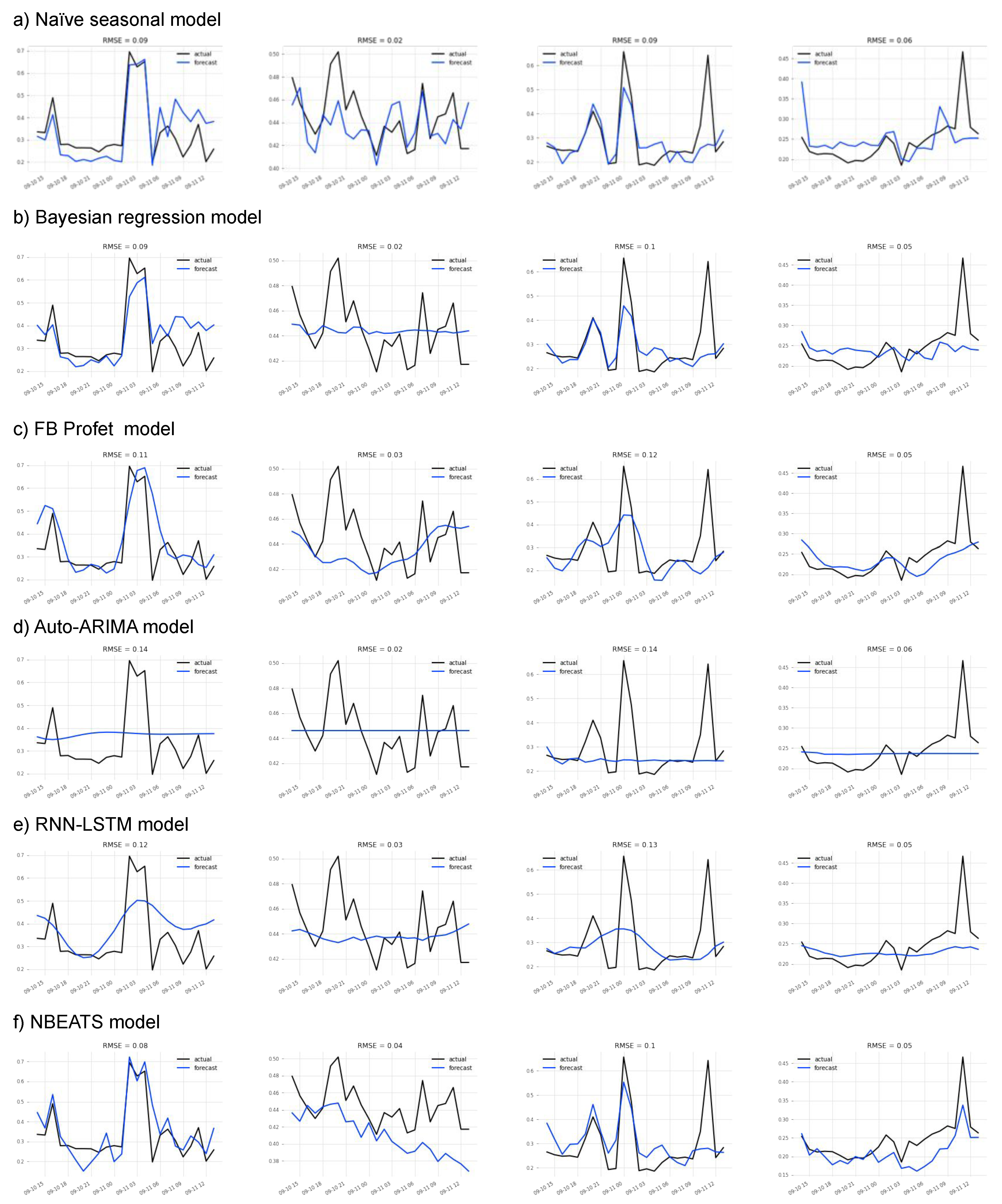
This work introduced a novel Smart 5G Edge-Cloud Management Architecture based on OpenNebula. The proposed architecture incorporates experimental components from the ONEedge5G project which, in its current developmental phase, will incorporate predictive intelligence mechanisms for CPU utilization forecasting and optimization algorithms for the optimal allocation of virtual resources (VMs or containers) on geographically distributed 5G edge infrastructures.
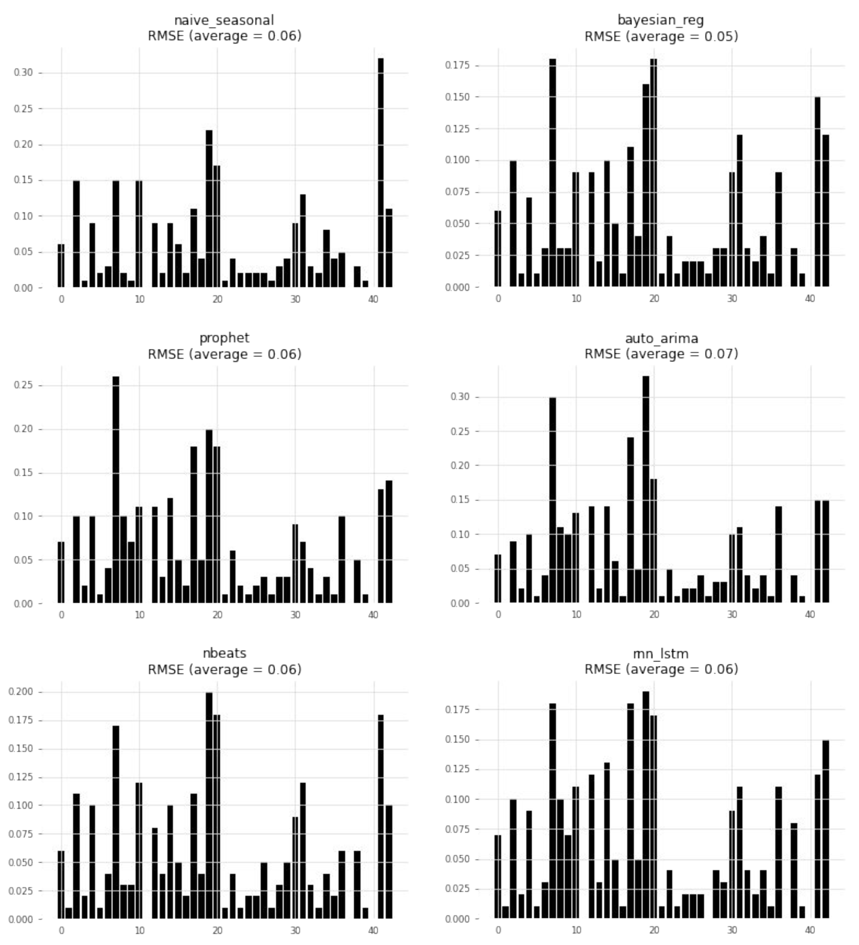
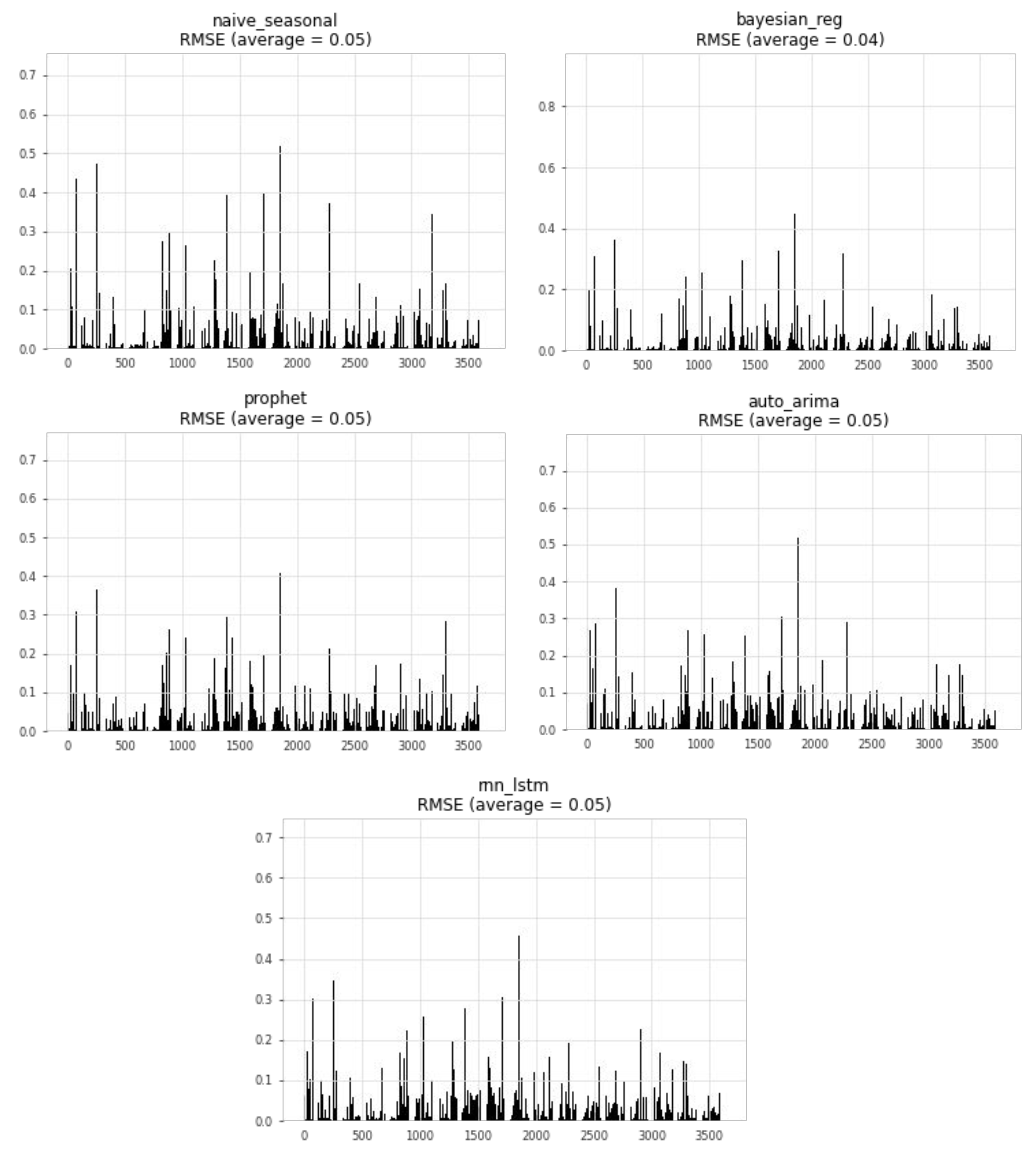
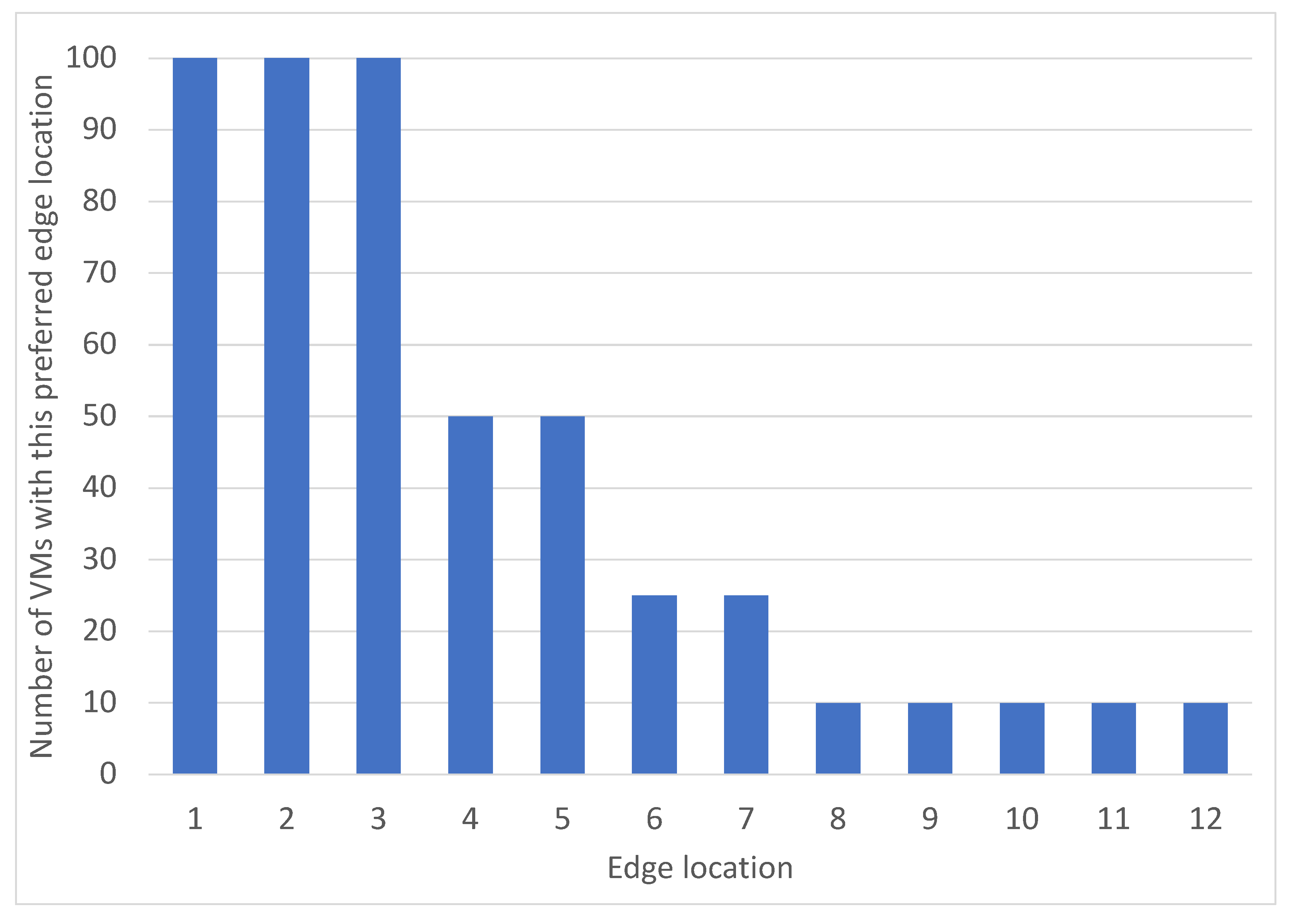
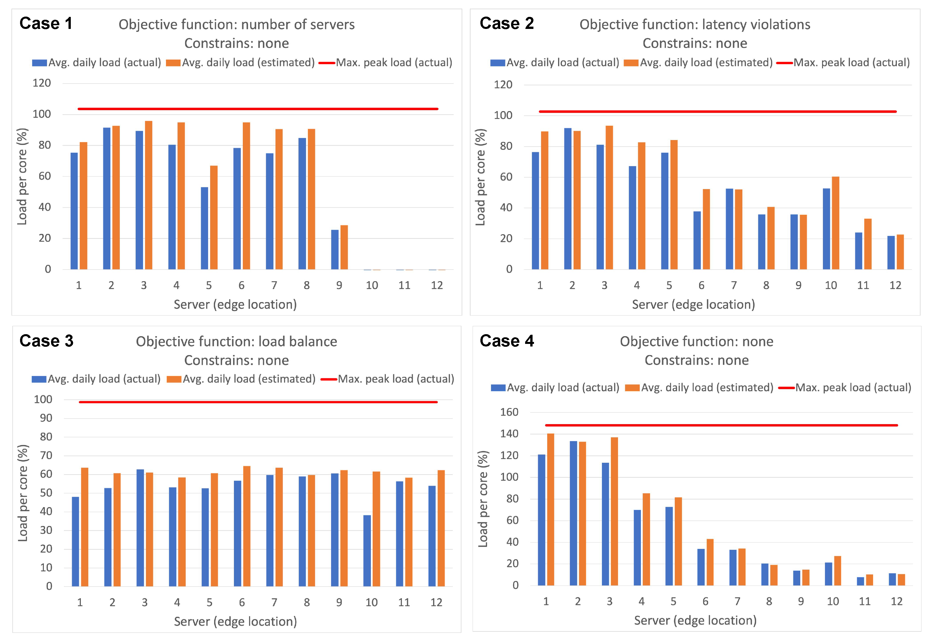
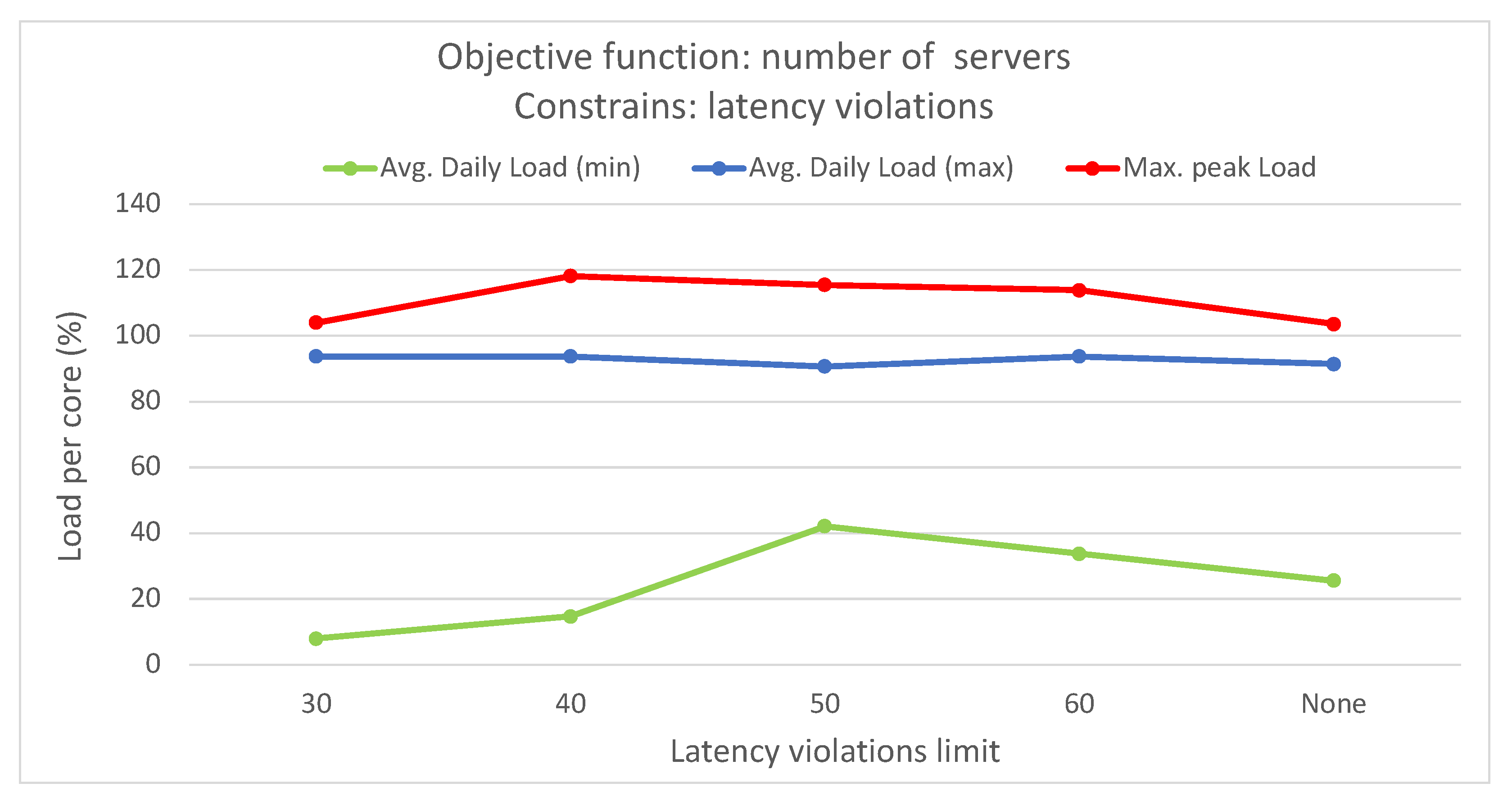
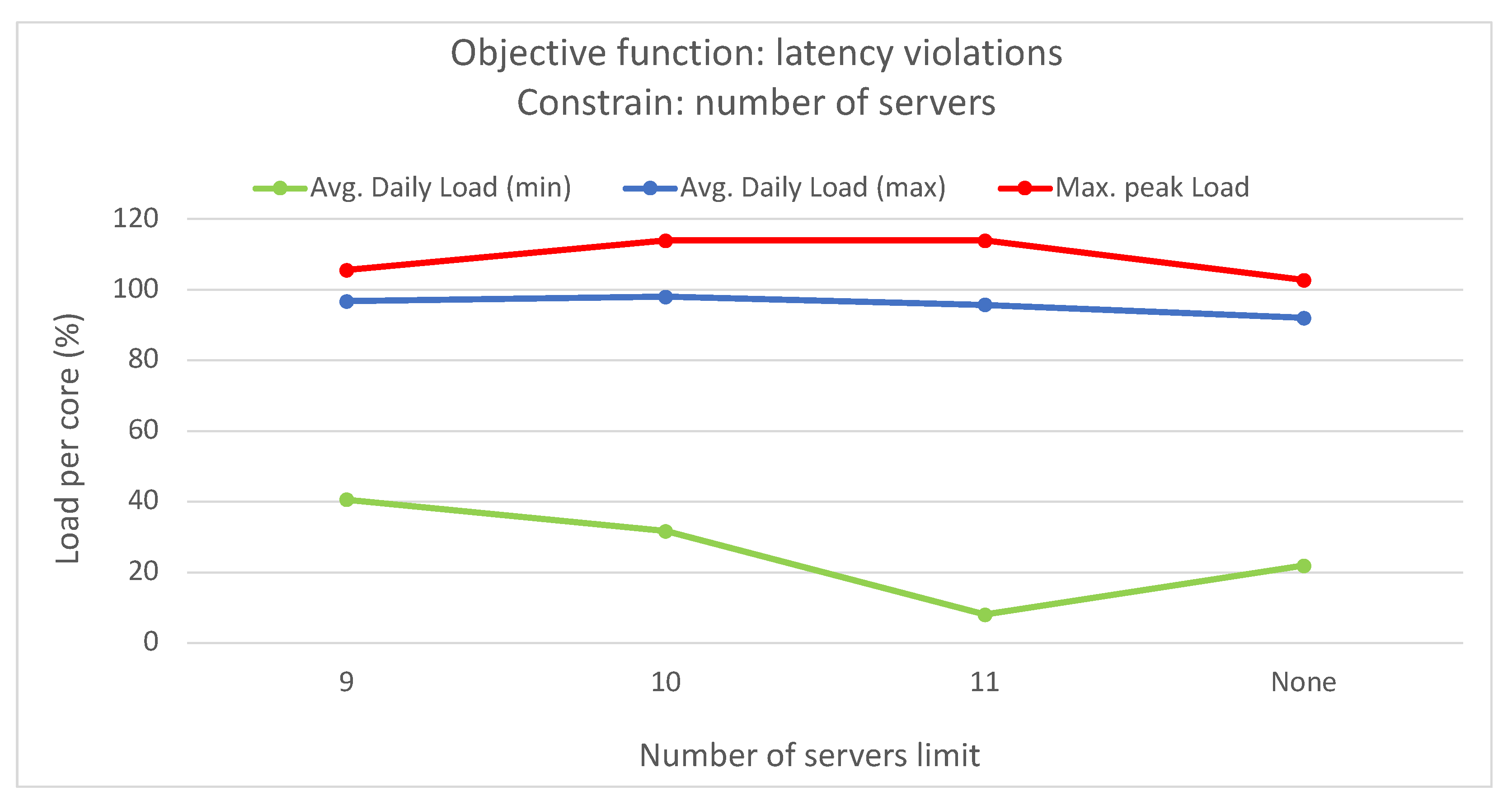
This study emphasized infrastructure-level techniques for CPU usage forecasting, employing different statistical and ML time-series forecasting methods. Bayesian regression demonstrated the highest accuracy among the methods evaluated. The optimization problem addressed involved finding the optimal mapping of virtual resources to edge servers using different criteria and constraints. An ILP formulation was proposed for solving this problem. The scenario included a distributed edge infrastructure with physical servers, each with specific computing and memory capacities. Virtual resources with their computing requirements, as well as preferred edge locations based on proximity criteria, were deployed in the infrastructure. The results showed that optimizing different objective functions, such as minimizing the number of servers, reducing latency violations, or balancing server loads, led to improved management of the infrastructure. Allocating virtual resources based on their preferred edge locations without optimization resulted in no latency violations but severe server overloading. However, optimization algorithms successfully prevented overloading, while maintaining an average daily load per server below 100%.
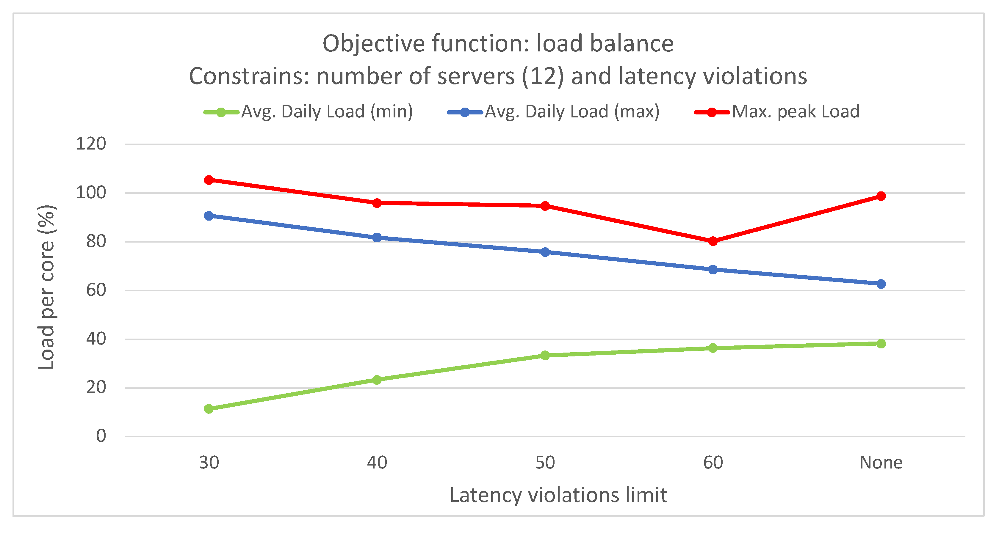
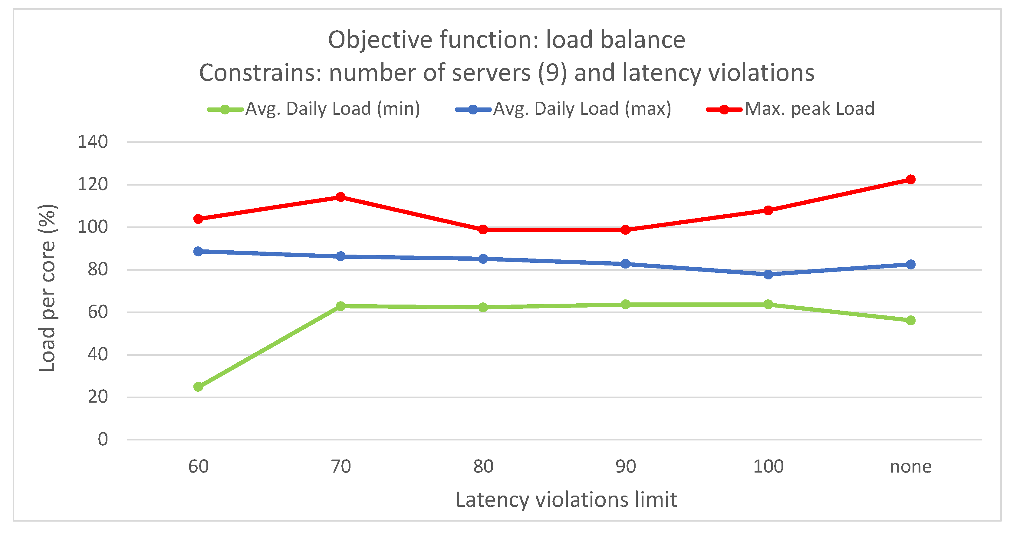
By merging various optimization criteria and constraints, such as the number of servers in use and the number of latency violations, different optimized solutions can be obtained. For instance, one approach is to minimize latency violations to a minimum of 29 by utilizing all available servers, while another option is to reduce the number of servers to nine with only 59 latency violations. However, these solutions introduce significant imbalances in load distribution among servers and may result in overloading on certain servers and time slots. To address this issue, incorporating the load balancing objective function proves effective, as it can achieve solutions with a limited number of latency violations, while improving load distribution and preventing overloading.
In our future work, we have various plans to enhance the prediction and optimization models. First, we aim to incorporate additional hardware metrics, including memory, bandwidth, and disk usage, to explore their potential correlation and integrate them into the mathematical models for optimization. Additionally, we plan to propose new optimization criteria based on the previous metrics, as well as integrating different objective functions using various multi-objective approaches. We also intend to investigate alternative optimization techniques, such as bio-inspired algorithms or reinforcement learning algorithms, to further improve the efficiency of the system. Another aspect not addressed in this study but worthy of consideration in future research is the potential utilization of nested virtualization, where containers are not run directly on bare-metal servers but within VMs. In such scenarios, two levels of allocation should be addressed: containers to VMs, and VMs to physical servers. Finally, expanding the capabilities of the ONEedge5G modules is on our agenda, encompassing functionality for capacity planning, prediction, and anomaly detection, as well as proactive auto-scaling mechanisms to facilitate elasticity management. These advancements will contribute to the comprehensive development of our Smart 5G Edge-Cloud Management Architecture and enable more robust and adaptive management of distributed 5G edge infrastructures.

Author Contributions

All authors participated in the definition of the architecture. R.M.-V. conceived the study, coordinated the research, conducted the experimental section, and drafted the manuscript. E.H., R.S.M. and I.M.L. also participated in the definition of the experimental scenarios and helped to refine the manuscript. All authors have read and agreed to the published version of the manuscript.

Funding

This work was supported by the Spanish Ministry for Digital Transformation and Civil Service through the UNICO I+D 6G Program, Project OneEdge5G-Intelligence and Automation for the Operation of Distributed Edge Systems on 5G Advanced Infrastructures (TSI-064200-2023-1), co-funded by the European Union—NextGenerationEU through the Recovery and Resilience Facility (RRF).

Data Availability Statement

Datasets used in this work are publicly available at the following links: Azure public datasets: https://github.com/Azure/AzurePublicDataset/blob/master/AzurePublicDatasetV1.md (accessed on 25 January 2024); GWA-T-12-Bitbrains datasets: http://gwa.ewi.tudelft.nl/datasets/gwa-t-12-bitbrains (accessed on 25 January 2024).

Conflicts of Interest

Ignacio M. Llorente and Rubén S. Montero are, respectively, an employee and an external collaborator of OpenNebula Systems company. The author declare no conflicts of interest.

Abbreviations

The following abbreviations are used in this manuscript:
ARAutoregression
ARIMAAuto-Regressive Integrated Moving Average
eMBBEnhanced Mobile Broadband
FBFacebook
AIArtificial Intelligence
ILPInteger Linear Programming
IoTInternet of Things
LSTMLong Short-Term Memory
MAMoving Average
MAEMean Absolute Error
MECMulti-access Edge Computing
MIMOMultiple-Input Multiple-Output
MLMachine Learning
mMTCMassive Machine Type Communication
MSEMean Squared Error
N-BEATSNeural Basis Expansion Analysis for Time Series
QoEQuality of Experience
QoSQuality of Service
RMSERoot Mean Squared Error
RNNRecurrent Neural Networks
SLAsService Level Agreements
UEUser Equipment
URLLCUltra-Reliable and Low-Latency Communication
VMVirtual Machine

References

  1. Huedo, E.; Montero, R.S.; Moreno-Vozmediano, R.; Vázquez, C.; Holer, V.; Llorente, I.M. Opportunistic Deployment of Distributed Edge Clouds for Latency-Critical Applications. J. Grid Comput. 2021, 19, 2. [Google Scholar] [CrossRef]
  2. Aral, A.; Brandic, I.; Uriarte, R.B.; Nicola, R.D.; Scoca, V. Addressing Application Latency Requirements through Edge Scheduling. J. Grid Comput. 2019, 17, 677–698. [Google Scholar] [CrossRef]
  3. Overbeek, D. Predictive DRS. Available online: https://blogs.vmware.com/management/2016/11/predictive-drs.html (accessed on 26 February 2024).
  4. Kralicky, J. Opni-Multi-Cluster Observability with AIOps. Available online: https://opni.io/ (accessed on 26 February 2024).
  5. Google Developers. Google Active Assist. Available online: https://cloud.google.com/recommender/docs/whatis-activeassist (accessed on 26 February 2024).
  6. OpenNebula Systems. ONEedge: An On-Demand Software-Defined Edge Computing Solution. Available online: https://oneedge.io/ (accessed on 26 February 2024).
  7. Milojičić, D.; Llorente, I.M.; Montero, R.S. OpenNebula: A Cloud Management Tool. IEEE Internet Comput. 2011, 15, 11–14. [Google Scholar] [CrossRef]
  8. OpenNebula Systems. OpenNebula: The Open Source Cloud & Edge Computing Platform. Available online: https://opennebula.io (accessed on 25 January 2024).
  9. Liu, B.; Zhu, P.; Li, J.; Wang, D.; You, X. Energy-Efficient Optimization in Distributed Massive MIMO Systems for Slicing eMBB and URLLC Services. IEEE Trans. Veh. Technol. 2023, 72, 10473–10487. [Google Scholar] [CrossRef]
  10. Filali, A.; Abouaomar, A.; Cherkaoui, S.; Kobbane, A.; Guizani, M. Multi-Access Edge Computing: A Survey. IEEE Access 2020, 8, 197017–197046. [Google Scholar] [CrossRef]
  11. Hassan, N.; Yau, K.L.A.; Wu, C. Edge Computing in 5G: A Review. IEEE Access 2019, 7, 127276–127289. [Google Scholar] [CrossRef]
  12. Raeisi-Varzaneh, M.; Dakkak, O.; Habbal, A.; Kim, B.S. Resource Scheduling in Edge Computing: Architecture, Taxonomy, Open Issues and Future Research Directions. IEEE Access 2023, 11, 25329–25350. [Google Scholar] [CrossRef]
  13. Sarah, A.; Nencioni, G.; Khan, M.M.I. Resource Allocation in Multi-access Edge Computing for 5G-and-beyond networks. Comput. Netw. 2023, 227, 109720. [Google Scholar] [CrossRef]
  14. Dai, Y.; Xu, D.; Zhang, K.; Lu, Y.; Maharjan, S.; Zhang, Y. Deep Reinforcement Learning for Edge Computing and Resource Allocation in 5G Beyond. In Proceedings of the 2019 IEEE 19th International Conference on Communication Technology (ICCT), Xi’an, China, 16–19 October 2019; pp. 866–870. [Google Scholar] [CrossRef]
  15. Chen, M.; Miao, Y.; Gharavi, H.; Hu, L.; Humar, I. Intelligent Traffic Adaptive Resource Allocation for Edge Computing-Based 5G Networks. IEEE Trans. Cogn. Commun. Netw. 2020, 6, 499–508. [Google Scholar] [CrossRef]
  16. Wang, S.; Chen, M.; Liu, X.; Yin, C.; Cui, S.; Vincent Poor, H. A Machine Learning Approach for Task and Resource Allocation in Mobile-Edge Computing-Based Networks. IEEE Internet Things J. 2021, 8, 1358–1372. [Google Scholar] [CrossRef]
  17. Wang, J.; Zhao, L.; Liu, J.; Kato, N. Smart Resource Allocation for Mobile Edge Computing: A Deep Reinforcement Learning Approach. IEEE Trans. Emerg. Top. Comput. 2021, 9, 1529–1541. [Google Scholar] [CrossRef]
  18. Šlapak, E.; Gazda, J.; Guo, W.; Maksymyuk, T.; Dohler, M. Cost-Effective Resource Allocation for Multitier Mobile Edge Computing in 5G Mobile Networks. IEEE Access 2021, 9, 28658–28672. [Google Scholar] [CrossRef]
  19. Masdari, M.; Khoshnevis, A. A survey and classification of the workload forecasting methods in cloud computing. Clust. Comput. 2020, 23, 2399–2424. [Google Scholar] [CrossRef]
  20. Yadav, A.; Kushwaha, S.; Gupta, J.; Saxena, D.; Singh, A.K. A Survey of the Workload Forecasting Methods in Cloud Computing. In Proceedings of the 3rd International Conference on Machine Learning, Advances in Computing, Renewable Energy and Communication (Lecture Notes in Electrical Engineering), Singapore, 10–11 December 2022; pp. 539–547. [Google Scholar] [CrossRef]
  21. Rawat, P.S.; Gupta, P. Application of Optimization Techniques in Cloud Resource Management. In Bio-Inspired Optimization in Fog and Edge Computing Environments; Auerbach Publications: New York, NY, USA, 2022; pp. 73–90. [Google Scholar] [CrossRef]
  22. Ghobaei-Arani, M.; Souri, A.; Rahmanian, A.A. Resource Management Approaches in Fog Computing: A Comprehensive Review. J. Grid Comput. 2019, 18, 1–42. [Google Scholar] [CrossRef]
  23. Gao, J.; Wang, H.; Shen, H. Machine Learning Based Workload Prediction in Cloud Computing. In Proceedings of the 29th International Conference on Computer Communications and Networks (ICCCN), Honolulu, HI, USA, 3–6 August 2020. [Google Scholar] [CrossRef]
  24. Devi, K.L.; Valli, S. Time series-based workload prediction using the statistical hybrid model for the cloud environment. Computing 2023, 105, 353–374. [Google Scholar] [CrossRef]
  25. Rezvani, M.; Akbari, M.K.; Javadi, B. Resource Allocation in Cloud Computing Environments Based on Integer Linear Programming. Comput. J. 2014, 58, 300–314. [Google Scholar] [CrossRef]
  26. Lu, J.; Zhao, W.; Zhu, H.; Li, J.; Cheng, Z.; Xiao, G. Optimal machine placement based on improved genetic algorithm in cloud computing. J. Supercomput. 2021, 78, 3448–3476. [Google Scholar] [CrossRef]
  27. Khan, T.; Tian, W.; Zhou, G.; Ilager, S.; Gong, M.; Buyya, R. Machine learning (ML)-centric resource management in cloud computing: A review and future directions. J. Netw. Comput. Appl. 2022, 204, 103405. [Google Scholar] [CrossRef]
  28. Gupta, P.; Goyal, M.K.; Chakraborty, S.; Elngar, A.A. Machine Learning and Optimization Models for Optimization in Cloud; Chapman and Hall/CRC: New York, NY, USA, 2022. [Google Scholar] [CrossRef]
  29. Djigal, H.; Xu, J.; Liu, L.; Zhang, Y. Machine and Deep Learning for Resource Allocation in Multi-Access Edge Computing: A Survey. IEEE Commun. Surv. Tutor. 2022, 24, 2449–2494. [Google Scholar] [CrossRef]
  30. Patsias, V.; Amanatidis, P.; Karampatzakis, D.; Lagkas, T.; Michalakopoulou, K.; Nikitas, A. Task Allocation Methods and Optimization Techniques in Edge Computing: A Systematic Review of the Literature. Future Internet 2023, 15, 254. [Google Scholar] [CrossRef]
  31. Liang, Q.; Zhang, J.; Zhang, Y.H.; Liang, J.M. The placement method of resources and applications based on request prediction in cloud data center. Inf. Sci. 2014, 279, 735–745. [Google Scholar] [CrossRef]
  32. Moreno-Vozmediano, R.; Montero, R.S.; Huedo, E.; Llorente, I.M. Efficient resource provisioning for elastic Cloud services based on machine learning techniques. J. Cloud Comput. 2019, 8, 1–18. [Google Scholar] [CrossRef]
  33. Mehmood, T.; Latif, S.; Malik, S. Prediction Of Cloud Computing Resource Utilization. In Proceedings of the 15th International Conference on Smart Cities: Improving Quality of Life Using ICT & IoT (HONET-ICT), Islamabad, Pakistan, 8–10 October 2018. [Google Scholar] [CrossRef]
  34. Al-Asaly, M.S.; Bencherif, M.A.; Alsanad, A.; Hassan, M.M. A deep learning-based resource usage prediction model for resource provisioning in an autonomic cloud computing environment. Neural Comput. Appl. 2021, 34, 10211–10228. [Google Scholar] [CrossRef]
  35. Aslanpour, M.S.; Gill, S.S.; Toosi, A.N. Performance evaluation metrics for cloud, fog and edge computing: A review, taxonomy, benchmarks and standards for future research. Internet Things 2020, 12, 100273. [Google Scholar] [CrossRef]
  36. Yang, J.; Liu, C.; Shang, Y.; Mao, Z.; Chen, J. Workload Predicting-Based Automatic Scaling in Service Clouds. In Proceedings of the 2013 IEEE Sixth International Conference on Cloud Computing, Santa Clara, CA, USA, 28 June–3 July 2013. [Google Scholar] [CrossRef]
  37. Di, S.; Kondo, D.; Cirne, W. Host load prediction in a Google compute cloud with a Bayesian model. In Proceedings of the 2012 International Conference for High Performance Computing, Networking, Storage and Analysis, Salt Lake City, UT, USA, 24–29 June 2012. [Google Scholar] [CrossRef]
  38. Calheiros, R.N.; Masoumi, E.; Ranjan, R.; Buyya, R. Workload Prediction Using ARIMA Model and Its Impact on Cloud Applications’ QoS. IEEE Trans. Cloud Comput. 2015, 3, 449–458. [Google Scholar] [CrossRef]
  39. Khan, T.; Tian, W.; Ilager, S.; Buyya, R. Workload forecasting and energy state estimation in cloud data centres: ML-centric approach. Future Gener. Comput. Syst. 2022, 128, 320–332. [Google Scholar] [CrossRef]
  40. Nawrocki, P.; Osypanka, P. Cloud Resource Demand Prediction using Machine Learning in the Context of QoS Parameters. J. Grid Comput. 2021, 19, 20. [Google Scholar] [CrossRef]
  41. Bi, J.; Li, S.; Yuan, H.; Zhou, M. Integrated deep learning method for workload and resource prediction in cloud systems. Neurocomputing 2021, 424, 35–48. [Google Scholar] [CrossRef]
  42. Chen, L.; Zhang, W.; Ye, H. Accurate workload prediction for edge data centers: Savitzky-Golay filter, CNN and BiLSTM with attention mechanism. Appl. Intell. 2022, 52, 13027–13042. [Google Scholar] [CrossRef]
  43. Tordsson, J.; Montero, R.S.; Moreno-Vozmediano, R.; Llorente, I.M. Cloud brokering mechanisms for optimized placement of virtual machines across multiple providers. Future Gener. Comput. Syst. 2012, 28, 358–367. [Google Scholar] [CrossRef]
  44. Lucas-Simarro, J.L.; Moreno-Vozmediano, R.; Montero, R.S.; Llorente, I.M. Scheduling strategies for optimal service deployment across multiple clouds. Future Gener. Comput. Syst. 2013, 29, 1431–1441. [Google Scholar] [CrossRef]
  45. Entrialgo, J.; Díaz, J.L.; García, J.; García, M.; García, D.F. Cost Minimization of Virtual Machine Allocation in Public Clouds Considering Multiple Applications. In Lecture Notes in Computer Science; Springer International Publishing: Cham, Switzerland, 2017; pp. 147–161. [Google Scholar] [CrossRef]
  46. Entrialgo, J.; García, M.; Díaz, J.L.; García, J.; García, D.F. Modelling and simulation for cost optimization and performance analysis of transactional applications in hybrid clouds. Simul. Model. Pract. Theory 2021, 109, 102311. [Google Scholar] [CrossRef]
  47. Fadda, E.; Plebani, P.; Vitali, M. Optimizing Monitorability of Multi-cloud Applications. In Lecture Notes in Computer Science; Springer International Publishing: Cham, Switzerland, 2016; pp. 411–426. [Google Scholar] [CrossRef]
  48. Fadda, E.; Plebani, P.; Vitali, M. Monitoring-Aware Optimal Deployment for Applications Based on Microservices. IEEE Trans. Serv. Comput. 2021, 14, 1849–1863. [Google Scholar] [CrossRef]
  49. Gong, Y. Optimal Edge Server and Service Placement in Mobile Edge Computing. In Proceedings of the 2020 IEEE 9th Joint International Information Technology and Artificial Intelligence Conference (ITAIC), Chongqing, China, 11–13 December 2020; Volume 9, pp. 688–691. [Google Scholar] [CrossRef]
  50. Takeda, A.; Kimura, T.; Hirata, K. Joint optimization of edge server and virtual machine placement in edge computing environments. In Proceedings of the 2020 Asia-Pacific Signal and Information Processing Association Annual Summit and Conference (APSIPA ASC), Auckland, New Zealand, 7–10 December 2020; pp. 1545–1548. [Google Scholar]
  51. Abbasi, M.; Pasand, E.M.; Khosravi, M.R. Workload Allocation in IoT-Fog-Cloud Architecture Using a Multi-Objective Genetic Algorithm. J. Grid Comput. 2020, 18, 43–56. [Google Scholar] [CrossRef]
  52. Devarasetty, P.; Reddy, S. Genetic algorithm for quality of service based resource allocation in cloud computing. Evol. Intell. 2019, 14, 381–387. [Google Scholar] [CrossRef]
  53. Xia, W.; Shen, L. Joint Resource Allocation at Edge Cloud Based on Ant Colony Optimization and Genetic Algorithm. Wirel. Pers. Commun. 2021, 117, 355–386. [Google Scholar] [CrossRef]
  54. Pradhan, A.; Bisoy, S.K.; Das, A. A survey on PSO based meta-heuristic scheduling mechanism in cloud computing environment. J. King Saud Univ.-Comput. Inf. Sci. 2022, 34, 4888–4901. [Google Scholar] [CrossRef]
  55. Wang, B.; Liu, F.; Lin, W. Energy-efficient VM scheduling based on deep reinforcement learning. Future Gener. Comput. Syst. 2021, 125, 616–628. [Google Scholar] [CrossRef]
  56. Jiang, Y.; Kodialam, M.; Lakshman, T.V.; Mukherjee, S.; Tassiulas, L. Resource Allocation in Data Centers Using Fast Reinforcement Learning Algorithms. IEEE Trans. Netw. Serv. Manag. 2021, 18, 4576–4588. [Google Scholar] [CrossRef]
  57. Hummaida, A.R.; Paton, N.W.; Sakellariou, R. Scalable Virtual Machine Migration using Reinforcement Learning. J. Grid Comput. 2022, 20, 15. [Google Scholar] [CrossRef]
  58. Prometheus authors. Prometheus: From Metrics to Insight. Available online: https://prometheus.io (accessed on 25 January 2024).
  59. Unit8 SA. Darts: Time Series Made Easy in Python. Available online: https://unit8co.github.io/darts (accessed on 25 January 2024).
  60. Unit8 SA. Darts Baseline Models. Available online: https://unit8co.github.io/darts/generated_api/darts.models.forecasting.baselines.html (accessed on 25 January 2024).
  61. Box, G.E.P.; Jenkins, G.M.; Reinsel, G.C. Time Series Analysis; Wiley: Hoboken, NY, USA, 2008. [Google Scholar] [CrossRef]
  62. Smith, T.G. Alkaline-ML API Reference (pdmarima.arima.auto-arima). Available online: https://alkaline-ml.com/pmdarima/modules/generated/pmdarima.arima.auto_arima.html (accessed on 25 January 2024).
  63. Box, G.E.; Tiao, G.C. Bayesian Inference in Statistical Analysis; John Wiley & Sons, Inc.: New York, NY, USA, 1992. [Google Scholar] [CrossRef]
  64. Scikit-Learn Developers. Bayesian Ridge Regression. Available online: https://scikit-learn.org/0.24/modules/linear_model.html#bayesian-ridge-regression (accessed on 25 January 2024).
  65. Facebook Open Source. Prophet: Forecasting at Scale. Available online: https://facebook.github.io/prophet (accessed on 25 January 2024).
  66. Hochreiter, S.; Schmidhuber, J. Long Short-Term Memory. Neural Comput. 1997, 9, 1735–1780. [Google Scholar] [CrossRef] [PubMed]
  67. Oreshkin, B.N.; Carpov, D.; Chapados, N.; Bengio, Y. N-BEATS: Neural basis expansion analysis for interpretable time series forecasting. In Proceedings of the International Conference on Learning Representations, Addis Ababa, Ethiopia, 26 April–1 May 2020. [Google Scholar]
  68. Wilkes, J. The Google Workload Cluster Traces. Available online: https://github.com/google/cluster-data (accessed on 25 January 2024).
  69. Cortez, E. The Azure Public Dataset. Available online: https://github.com/Azure/AzurePublicDataset (accessed on 25 January 2024).
  70. Delft University of Technology. The Grid Workloads Archive: GWA-T-12 Bitbrains. Available online: http://gwa.ewi.tudelft.nl (accessed on 25 January 2024).
  71. Ding, H. The Alibaba Cluster Trace Program. Available online: https://github.com/alibaba/clusterdata (accessed on 25 January 2024).
  72. Nudler, E. Predator: Distributed Open-Source Performance Testing Platform for APIs. Available online: https://predator.dev (accessed on 25 January 2024).
  73. Heyman, J.; Byström, C.; Hamrén, J.; Heyman, H. Locust: A modern load testing framework. Available online: https://locust.io (accessed on 25 January 2024).
  74. Kolosov, O.; Yadgar, G.; Maheshwari, S.; Soljanin, E. Benchmarking in The Dark: On the Absence of Comprehensive Edge Datasets. In Proceedings of the 3rd USENIX Workshop on Hot Topics in Edge Computing (HotEdge 20). USENIX Association, Santa Clara, CA, USA, 25–26 June 2020. [Google Scholar]
  75. Tocze, K.; Schmitt, N.; Kargen, U.; Aral, A.; Brandic, I. Edge Workload Trace Gathering and Analysis for Benchmarking. In Proceedings of the 2022 IEEE 6th International Conference on Fog and Edge Computing (ICFEC), Messina, Italy, 18–19 May 2022. [Google Scholar] [CrossRef]
  76. Cortez, E.; Bonde, A.; Muzio, A.; Russinovich, M.; Fontoura, M.; Bianchini, R. Resource Central: Understanding and Predicting Workloads for Improved Resource Management in Large Cloud Platforms. In Proceedings of the SOSP’17: 26th Symposium on Operating Systems Principles, Shanghai, China, 28–31 October 2017; pp. 153–167. [Google Scholar] [CrossRef]
  77. Shen, S.; Beek, V.V.; Iosup, A. Statistical Characterization of Business-Critical Workloads Hosted in Cloud Datacenters. In Proceedings of the 2015 15th IEEE/ACM International Symposium on Cluster, Cloud and Grid Computing, Shenzhen, China, 4–7 May 2015; pp. 465–474. [Google Scholar] [CrossRef]
  78. Matthew, S.; Stefan, V.; Lou, H.; John, F.; Miles, L.; Ted, R.; Haroldo, G.S.; Samuel, B.; Bjarni, K.; Bruno, P.; et al. coin-or/Cbc: Release Releases/2.10.8. Available online: https://zenodo.org/records/6522795 (accessed on 25 January 2024).
  79. Cplex IBM ILOG. V12.1: User’s Manual for CPLEX. Int. Bus. Mach. Corp. 2009, 46, 157. [Google Scholar]
  80. Bestuzheva, K.; Besançon, M.; Chen, W.K.; Chmiela, A.; Donkiewicz, T.; van Doornmalen, J.; Eifler, L.; Gaul, O.; Gamrath, G.; Gleixner, A.; et al. The SCIP Optimization Suite 8.0. arXiv 2021, arXiv:2112.08872. [Google Scholar]
  81. Google for Developers. Get Started with OR-Tools for Python. Available online: https://developers.google.com/optimization/introduction/python (accessed on 25 January 2024).
  82. Google for Developers. OR-Tools Python Reference: Linear Solver (Pywraplp Module). Available online: https://developers.google.com/optimization/reference/python/linear_solver/pywraplp (accessed on 25 January 2024).
Figure 1. OpenNebula + ONEedge5G for intelligent orchestration of multiple 5G edge locations.
Futureinternet 16 00103 g001
Figure 2. Smart 5G Edge-Cloud Management Architecture.
Futureinternet 16 00103 g002
Figure 3. Distributed edge infrastructure.
Futureinternet 16 00103 g003
Figure 4. Forecasting results for a subset of Bitbrains VM traces (% CPU usage).
Futureinternet 16 00103 g004
Figure 5. Prediction accuracy (RMSE) of various time-series forecasting models applied to Bitbrains VM traces.
Futureinternet 16 00103 g005
Figure 6. Prediction accuracy (RMSE) of various time-series forecasting models applied to Azure VM traces.
Futureinternet 16 00103 g006
Figure 7. Distribution of VMs according to the preferred edge location.
Futureinternet 16 00103 g007
Figure 8. Estimated vs. actual load.
Futureinternet 16 00103 g008
Figure 9. Actual load per core for the ‘number of servers’ objective function under different latency violation constraints.
Futureinternet 16 00103 g009
Figure 10. Actual load per core for the ‘latency violations’ objective function under different server constraints.
Futureinternet 16 00103 g010
Figure 11. Actual load per core for the ‘load balancing’ objective function under different latency violation constrains and a server limit of 12.
Futureinternet 16 00103 g011
Figure 12. Actual load per core for the ‘load balancing’ objective function under different latency violation constrains and a server limit of 9.
Futureinternet 16 00103 g012
Figure 13. Sensitivity analysis results (actual load per core).
Futureinternet 16 00103 g013
Table 1. Summary of prediction accuracy (average RMSE) for Bitbrains traces.
ModelRMSE (Avg.)Exec. Time (Fit + Predict)
Naive seasonal0.061333 s
Bayesian Regression0.053636 s
FB Prophet0.062775 s
Auto-ARIMA0.07317 min
RNN-LSTM0.061923 min
N-BEATS0.05801 h
Adaptive (oracle)0.0455
Adaptive (realistic)0.0584
Table 2. Summary of prediction accuracy (average RMSE) for Azure traces.
ModelRMSE (Avg.)Exec. Time (Fit + Predict)
Naive seasonal (K = 24)0.049817 min.
Bayesian Regression0.041921 min.
FB Prophet0.050440 min.
Auto-ARIMA0.05085.9 h
RNN-LSTM0.049112.7 h
Adaptive (oracle)0.0314
Adaptive (realistic)0.0414
Table 3. Allocation results for different objective functions (without optional constraints).
CaseObjective FunctionTotal ServersTotal Lat. ViolationsSolver Exec. Time
1Number of servers93890.9 s
2Latency violations12291.0 s
3Load balance124321.4 s
4None120-
Table 4. Allocation results for the ‘number of servers’ objective function under different latency violation constraints.
Limit on Latency ViolationsTotal Servers UsedTotal Latency ViolationsSolver Exec. Time
3012303.2 s
40114010.7 s
50105018.6 s
6096010.6 s
None93890.9 s
Table 5. Allocation results for the ‘latency violations’ objective function under different server constraints.
Limit on Number of ServersTotal Servers UsedTotal Latency ViolationsSolver Exec. Time
99598.9 s
1010507.1 s
1111403.0 s
1212291.0 s
Table 6. Sensitivity analysis for the ‘number of servers’ objective function with no optional constraints.
CPU Usage Values Used for the OptimizationTotal Servers Used
Actual values8
Predicted values (lower bound)8
Predicted values (mean)9
Predicted values (upper bound)10
Disclaimer/Publisher’s Note: The statements, opinions and data contained in all publications are solely those of the individual author(s) and contributor(s) and not of MDPI and/or the editor(s). MDPI and/or the editor(s) disclaim responsibility for any injury to people or property resulting from any ideas, methods, instructions or products referred to in the content.

