
Using Computer Vision to Collect Information on Cycling and Hiking Trails Users

 and
and 
Abstract
:1. Introduction
2. Related Work
2.1. Research Questions
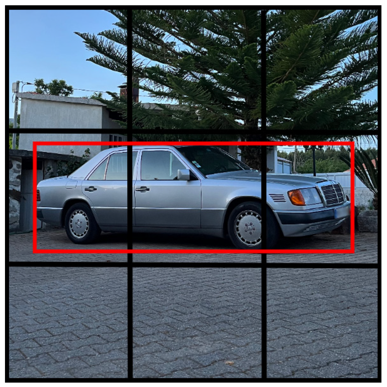
- Question No. 1—How can different types of users (cyclists and pedestrians) on cycling and hiking trails and routes be distinguished?
- Question No. 2—How can different types of users (cyclists and pedestrians) on cycling and hiking trails and routes be counted?
- Question No. 3—What frameworks exist for solutions to detect different types of users on cycling and hiking trails and routes?
2.2. Information Sources and Research Strategy
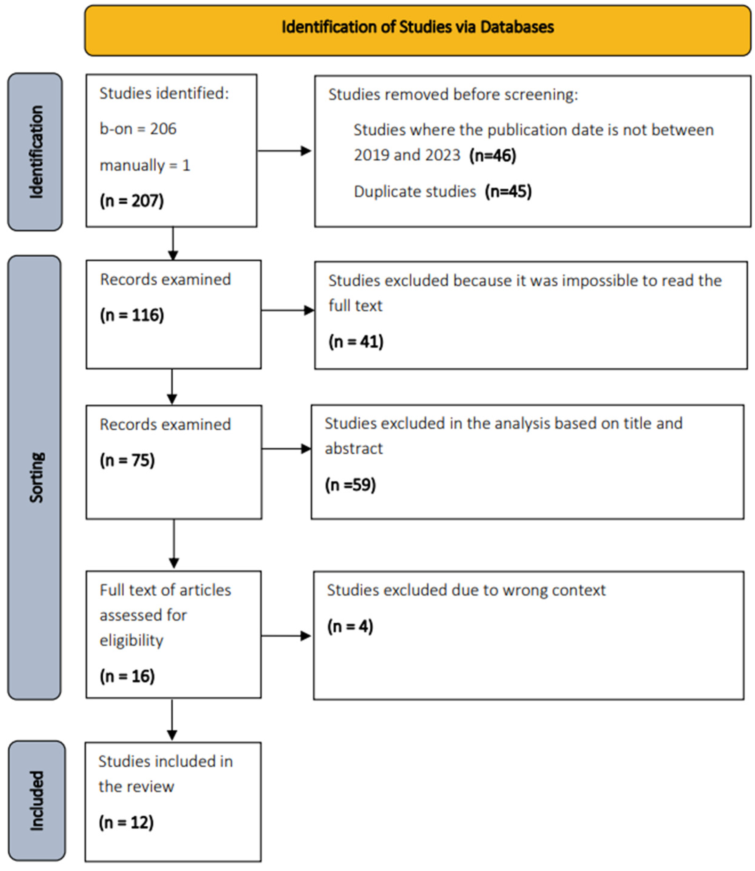
2.3. Selection Process
2.4. Analysis of Studies
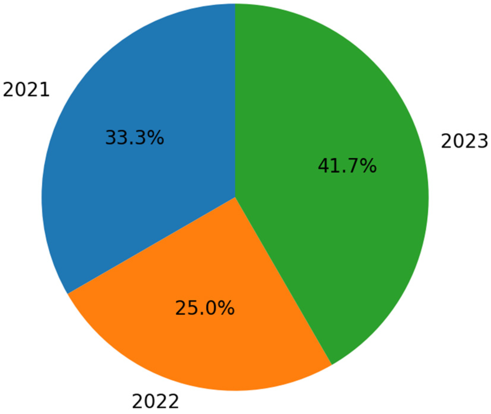
2.5. Results Obtained
2.6. Critical Analysis
- Question No. 1—How can different types of users (cyclists and pedestrians) on cycling and hiking trails and routes be distinguished?
- Question No. 2—How can different types of users (cyclists and pedestrians) on cycling and hiking trails and routes be counted?
- Question No. 3—What frameworks exist for solutions to detect different types of users on cycling and hiking trails and routes?
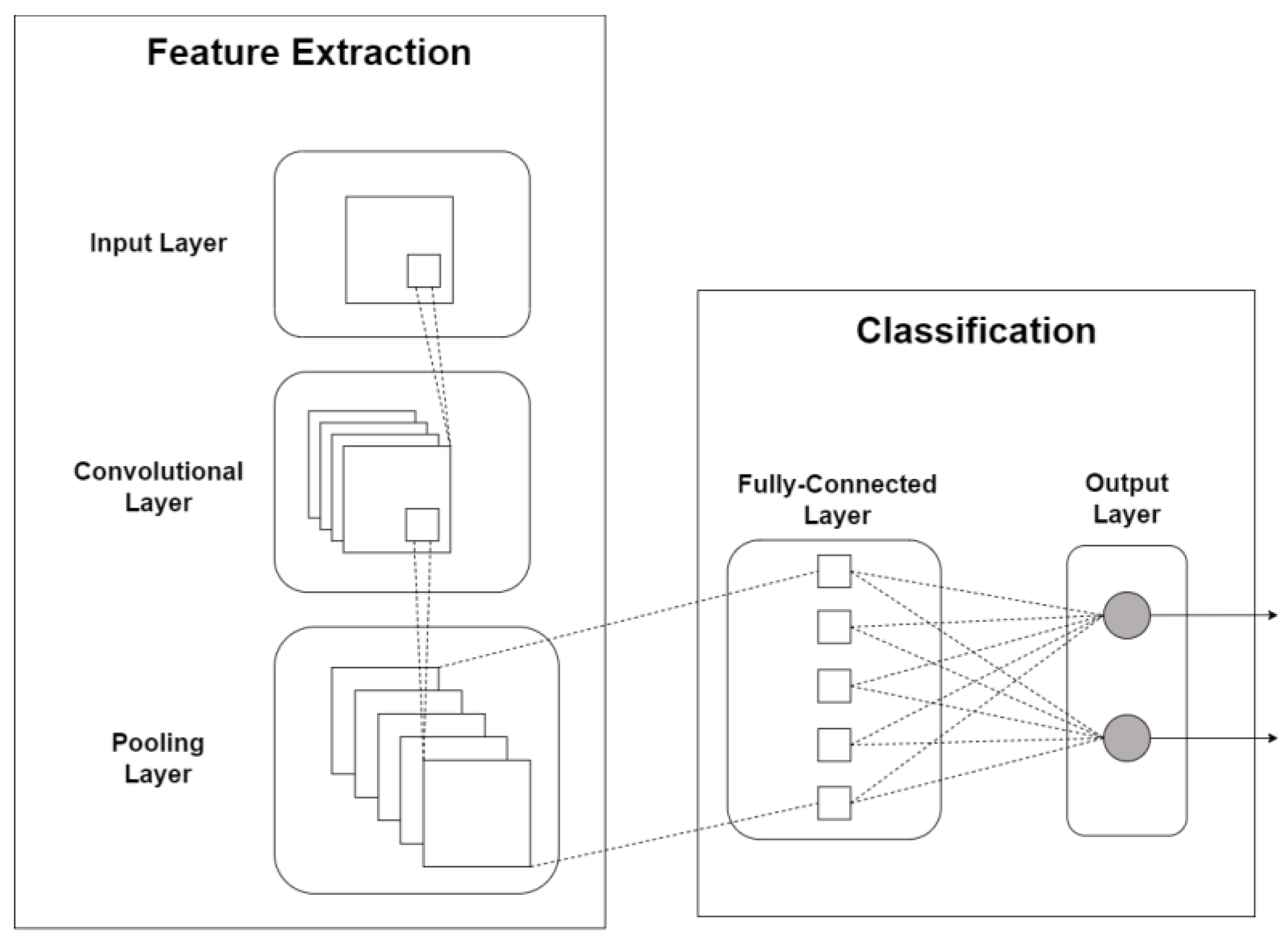
3. Computer Vision Techniques
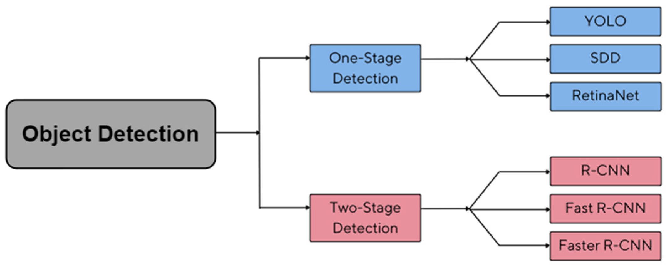
3.1. CNN Architectures
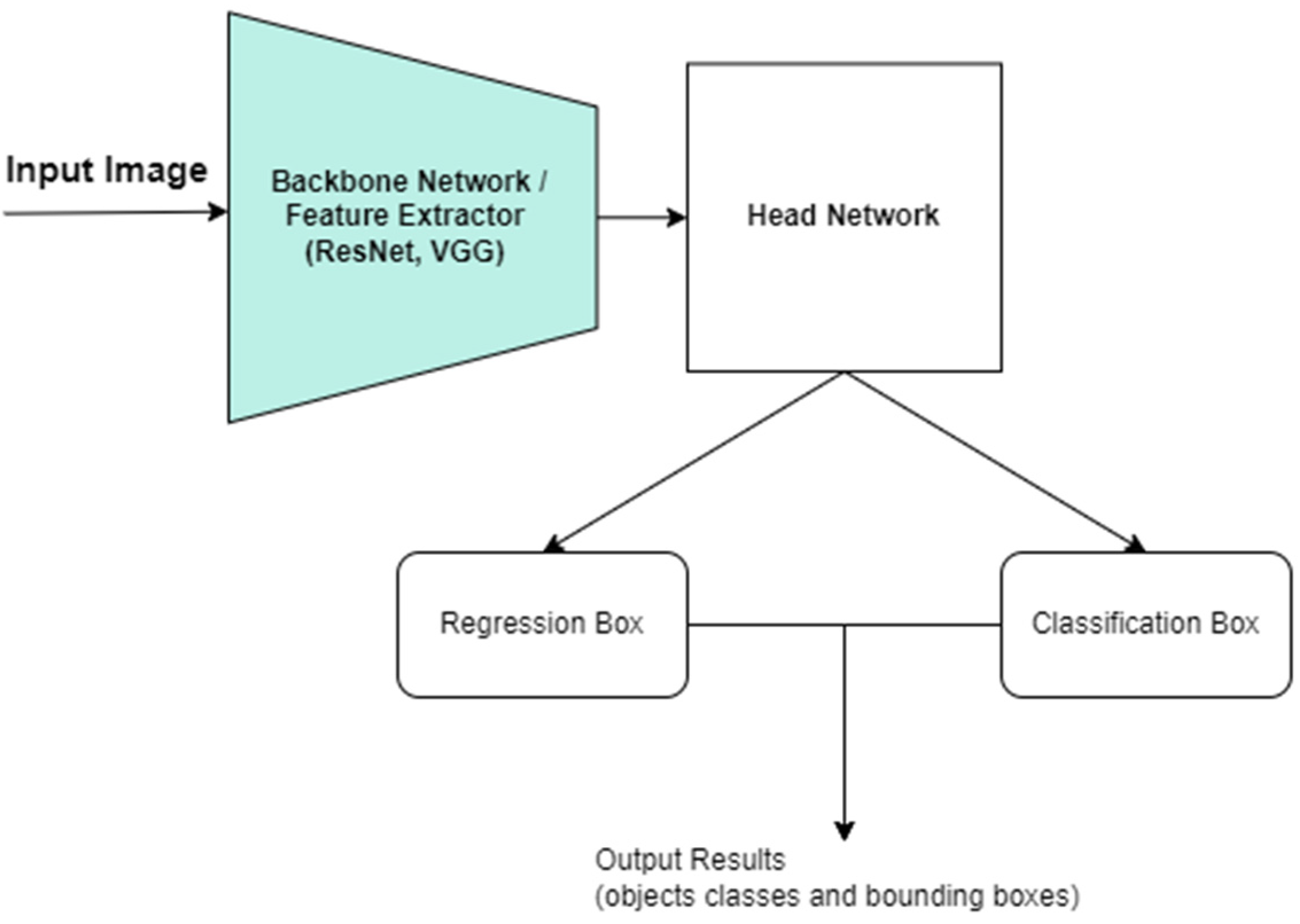
- One-Stage Detection
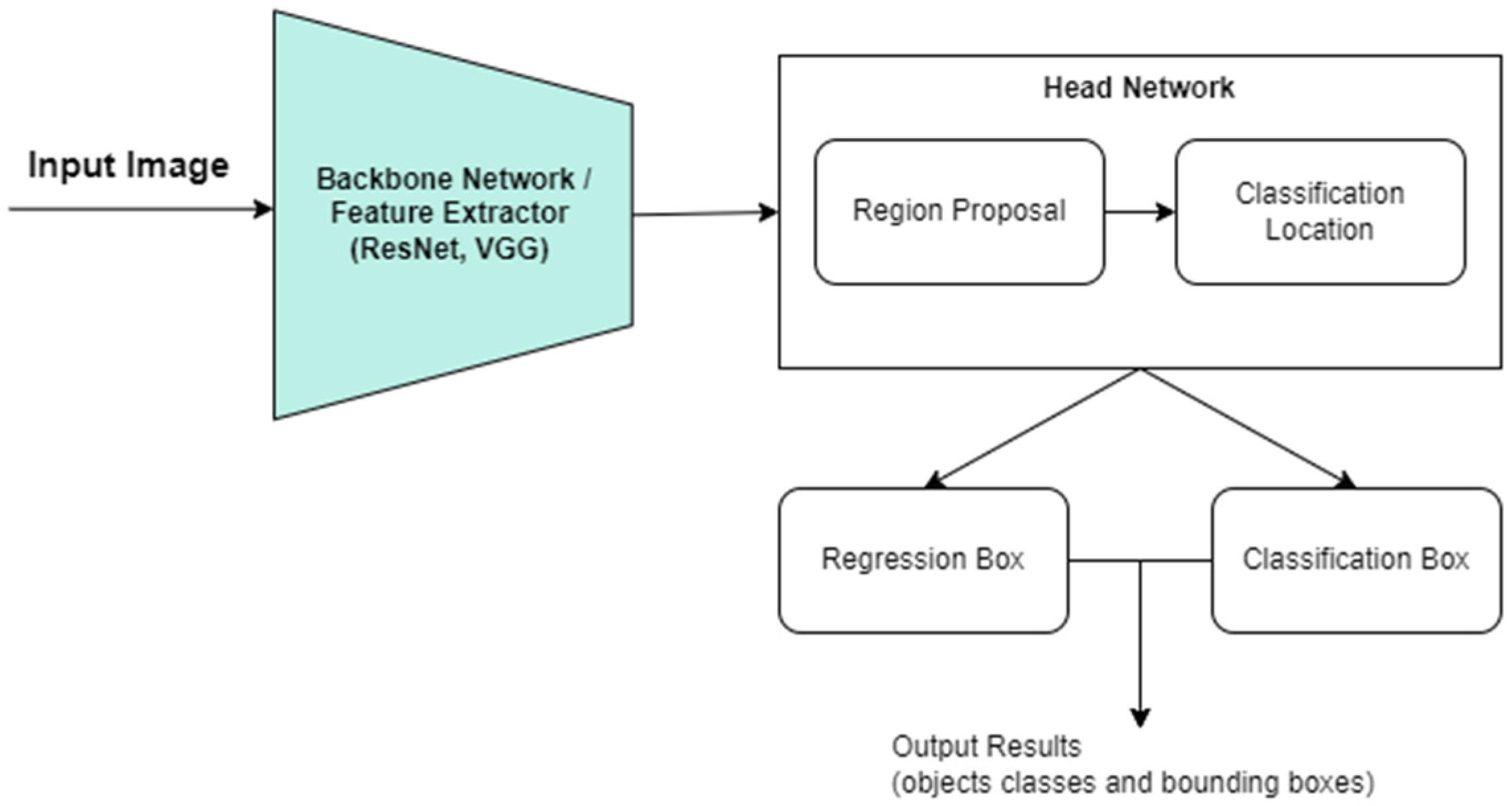
- Two-Stage Detection
3.2. CNN Model Analysis
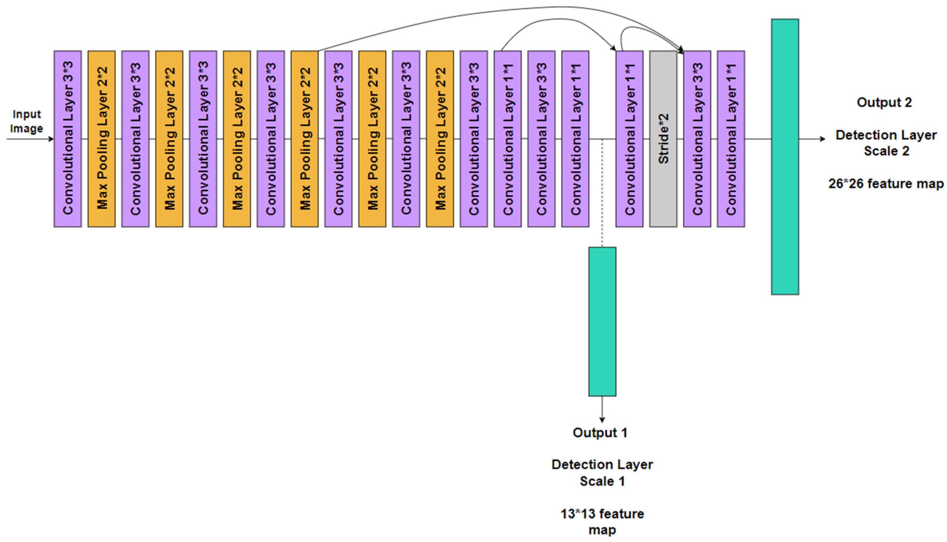
3.2.1. YOLOv3-Tiny
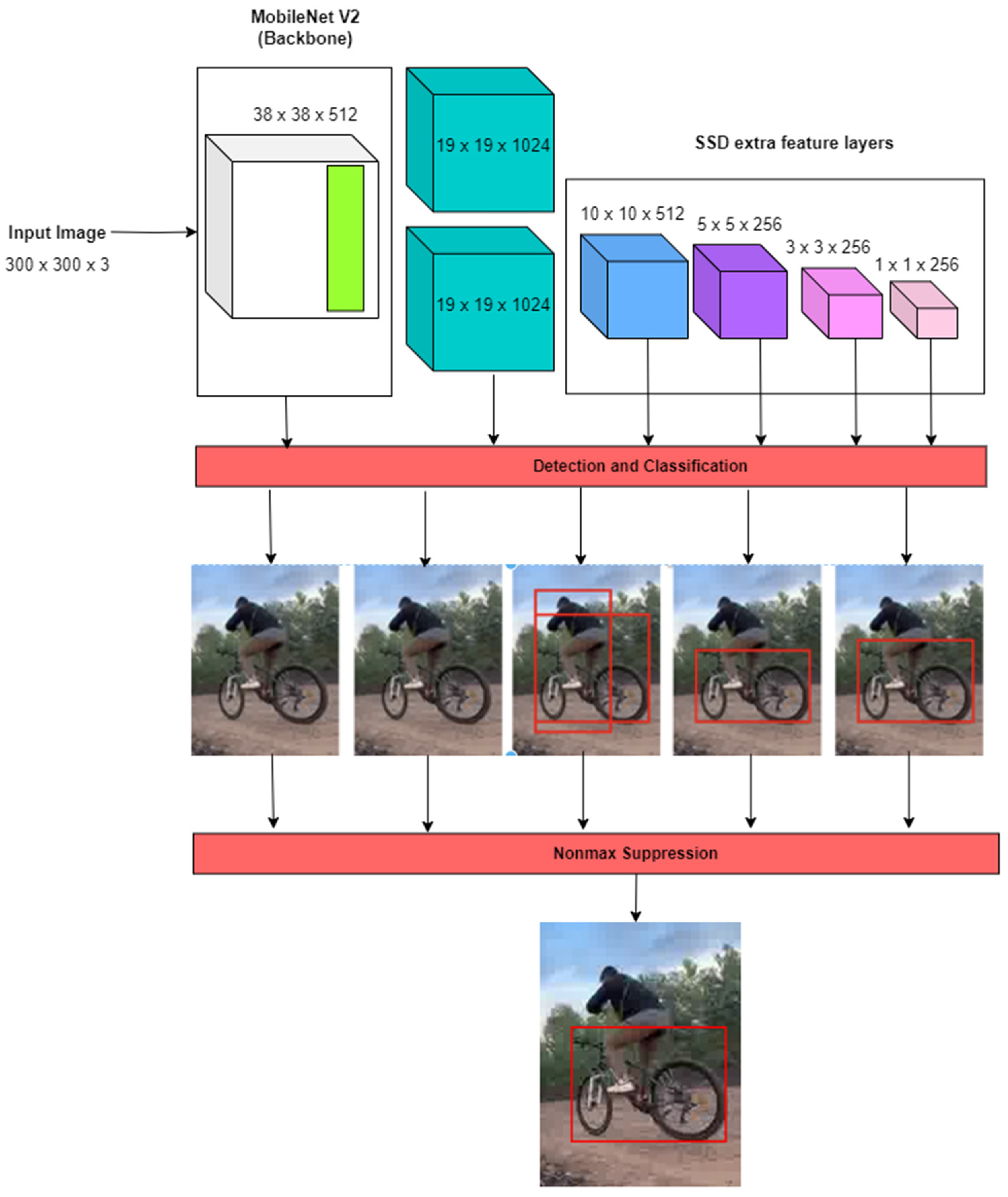
3.2.2. MobileNet-SSD V2
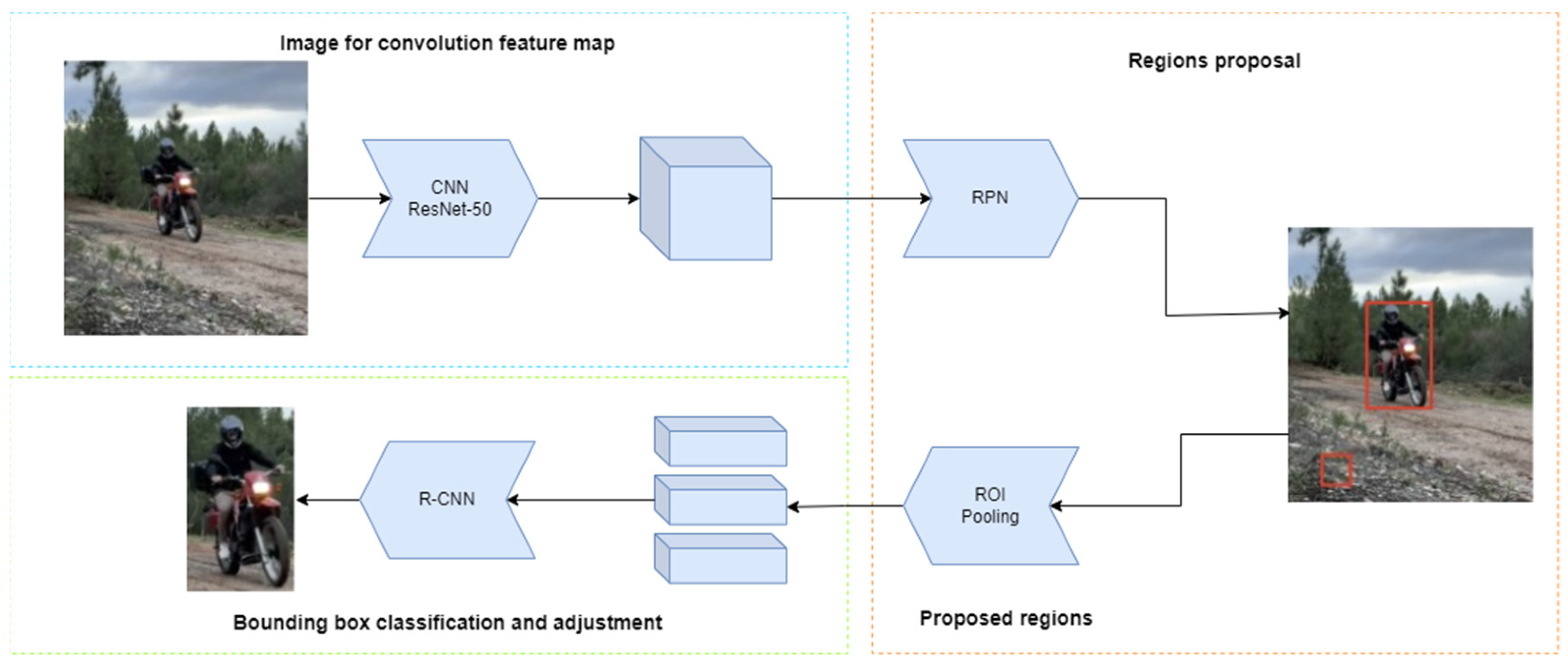
3.2.3. FasterRCNN and ResNet-50
4. Performance Evaluation
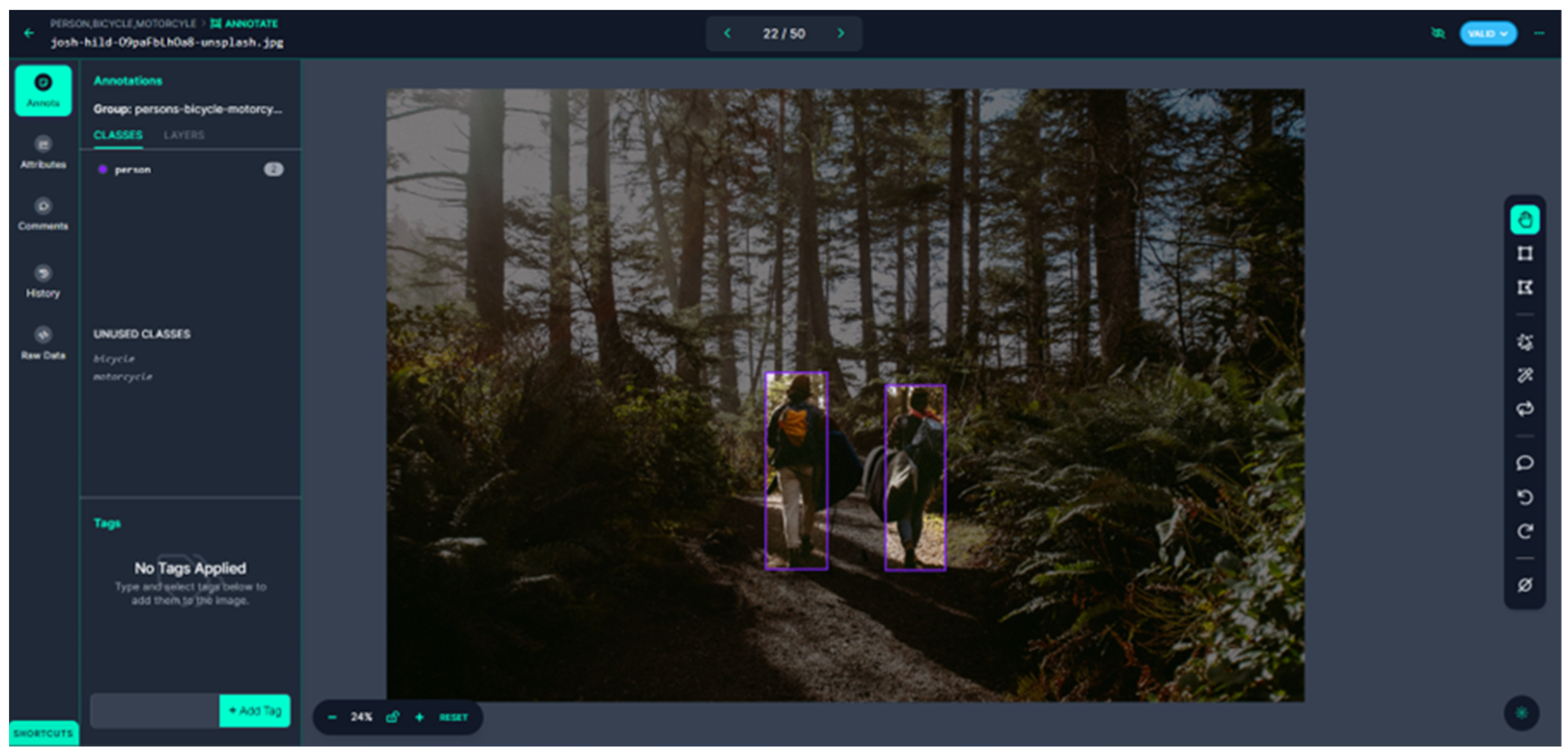
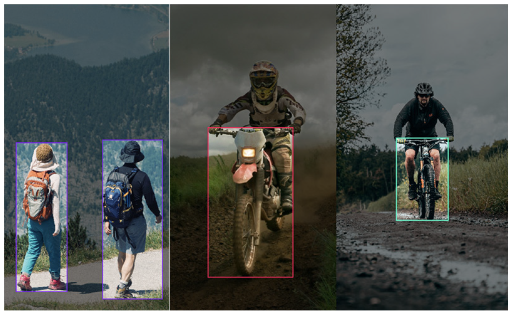
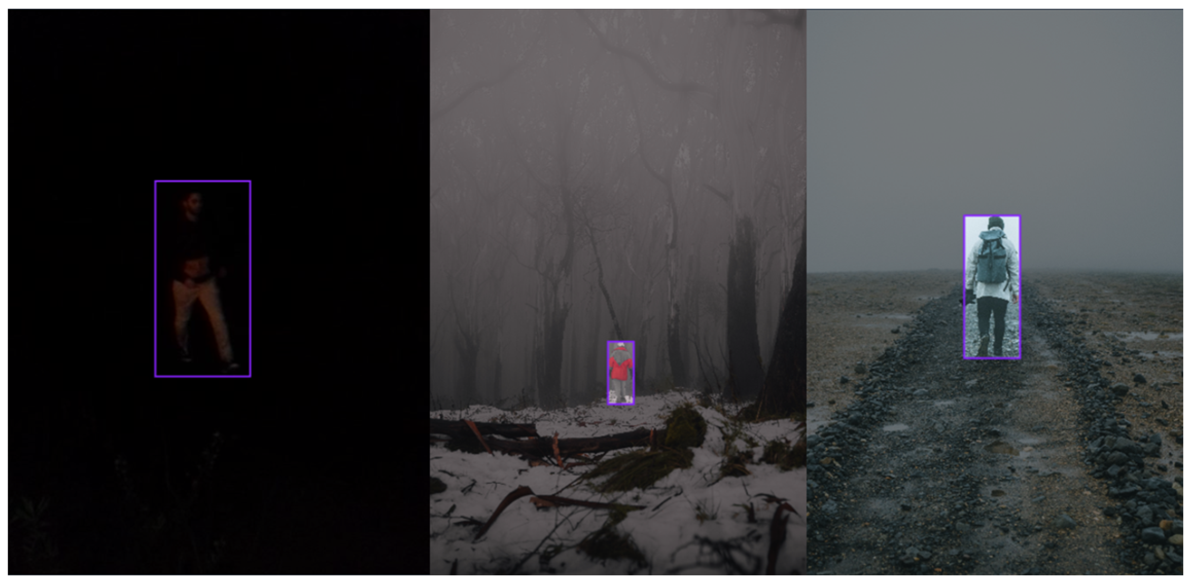
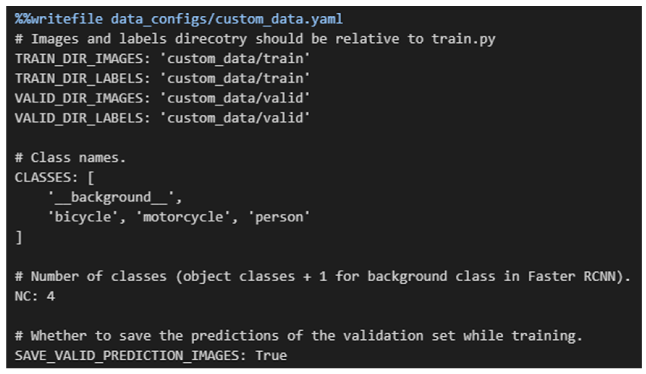
4.1. Dataset Description
4.2. Benchmark Scenario
4.3. Performance Metrics
4.4. Results and Discussion
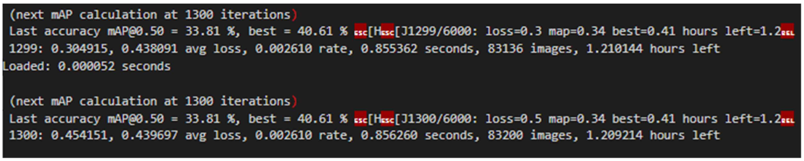
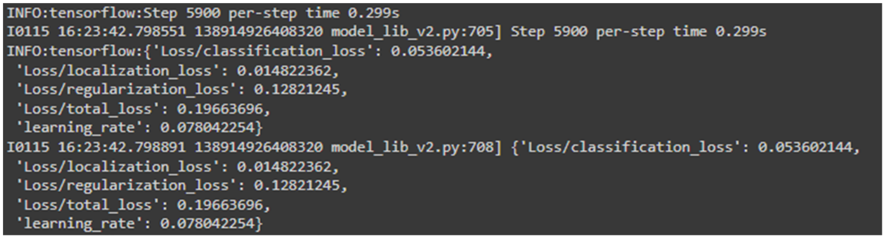
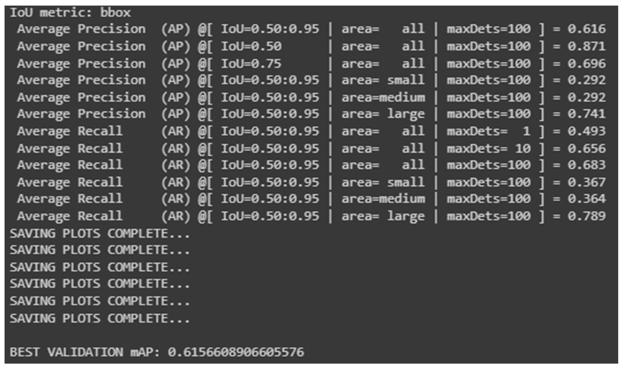
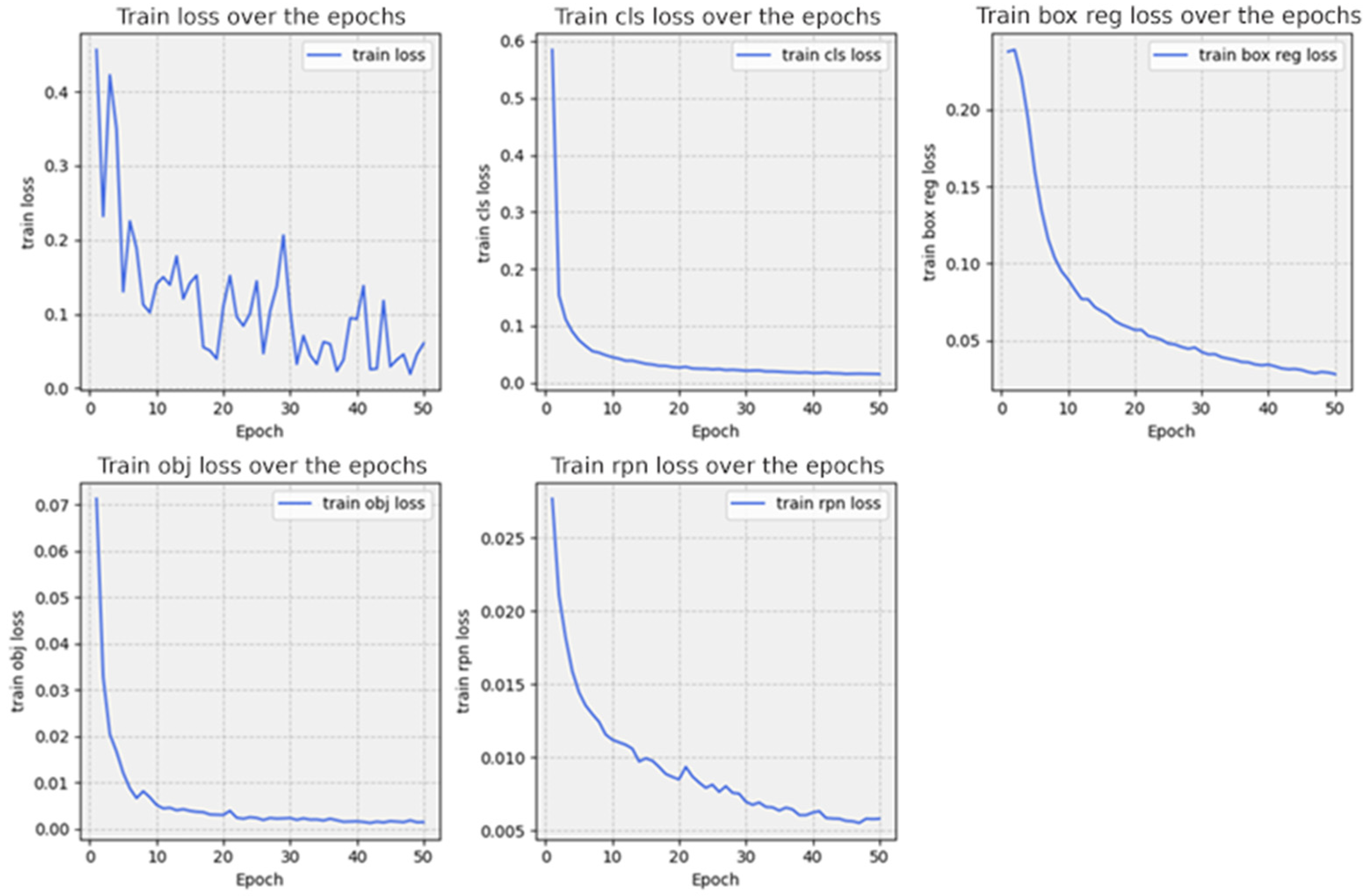
4.4.1. Train
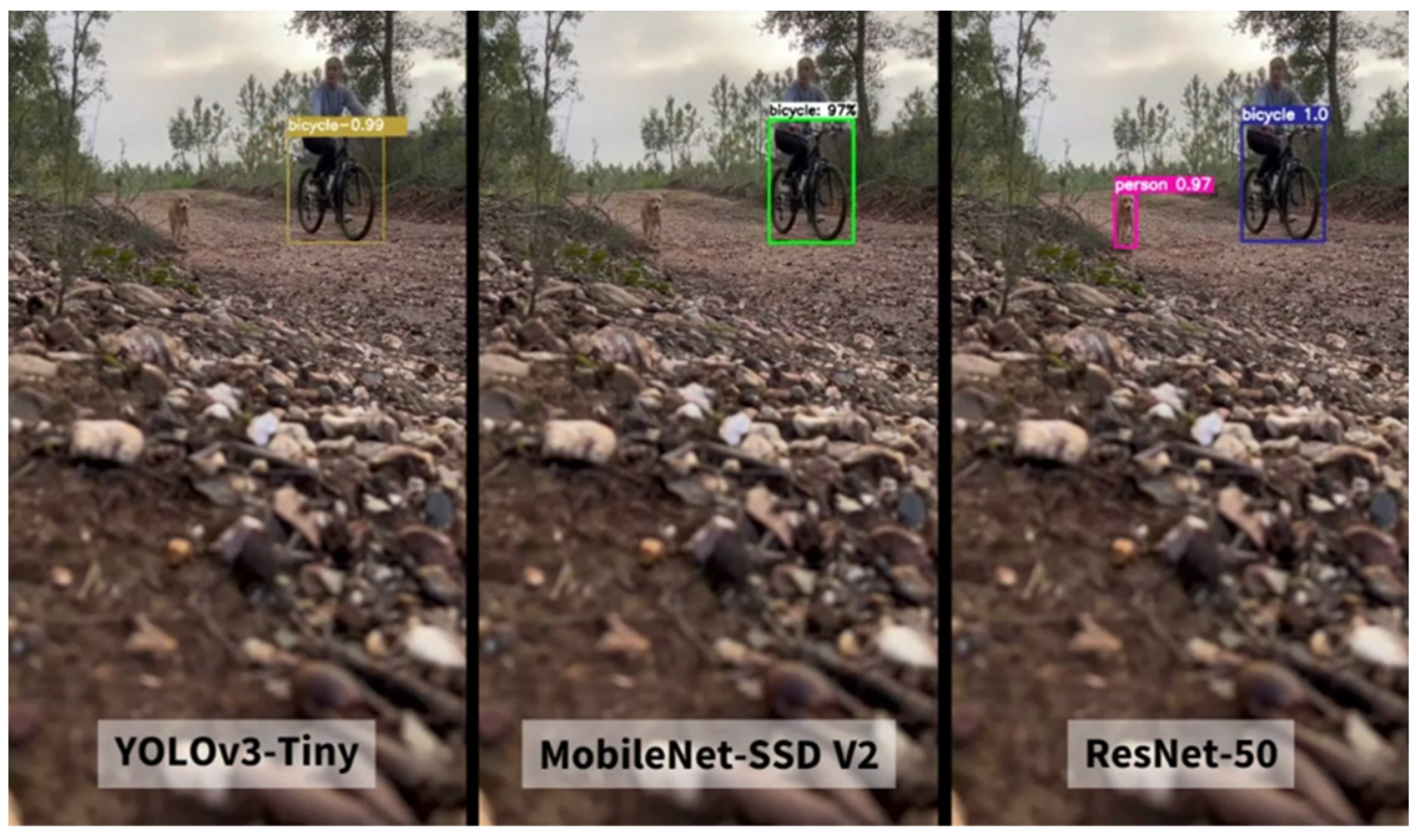
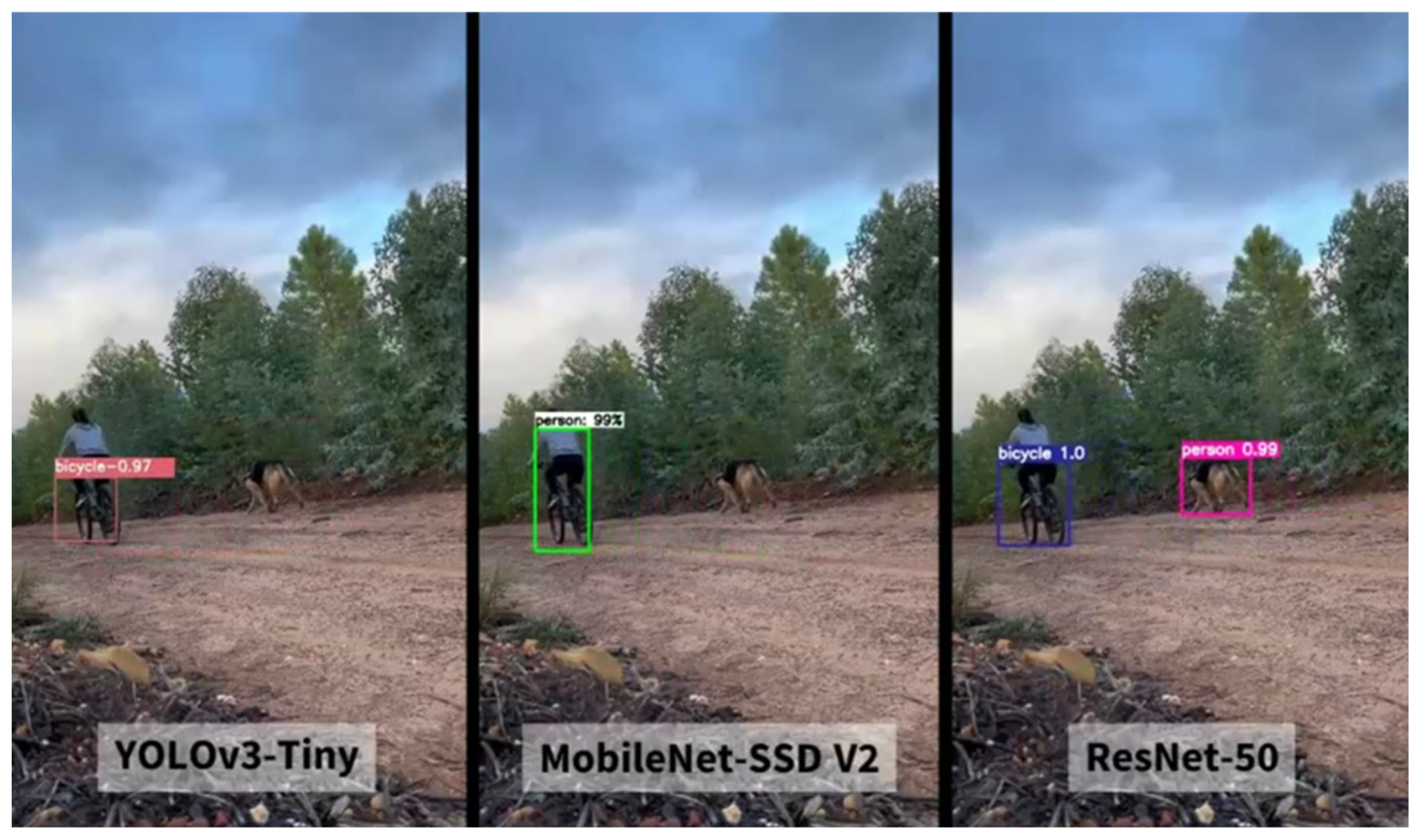
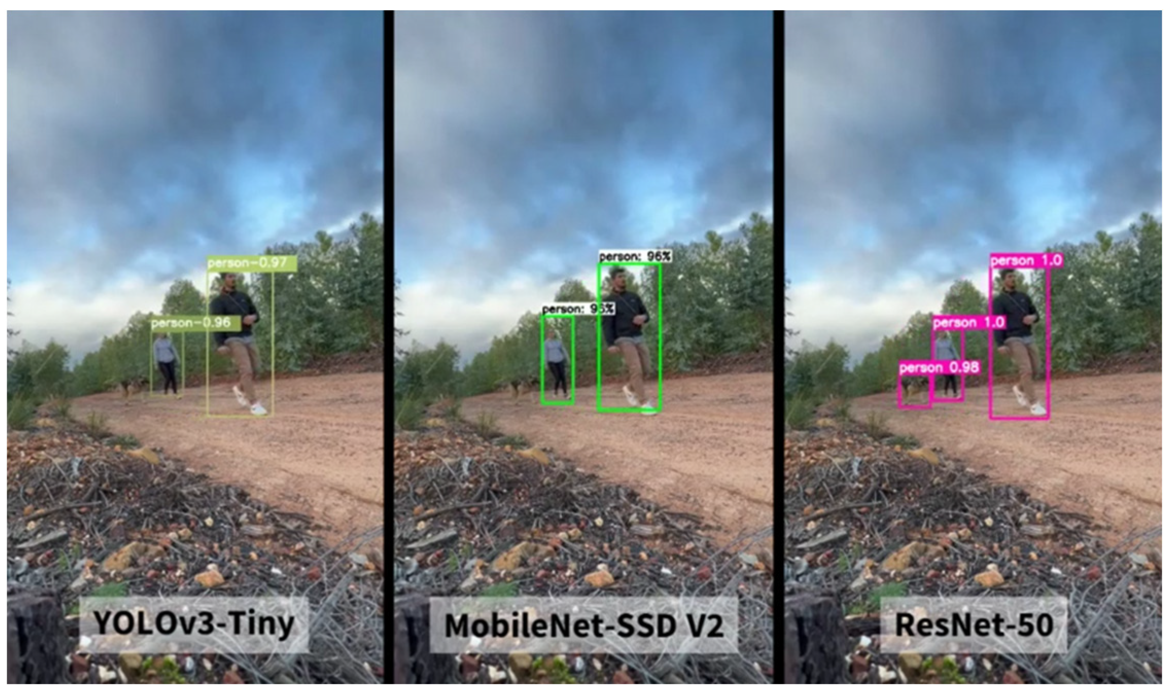
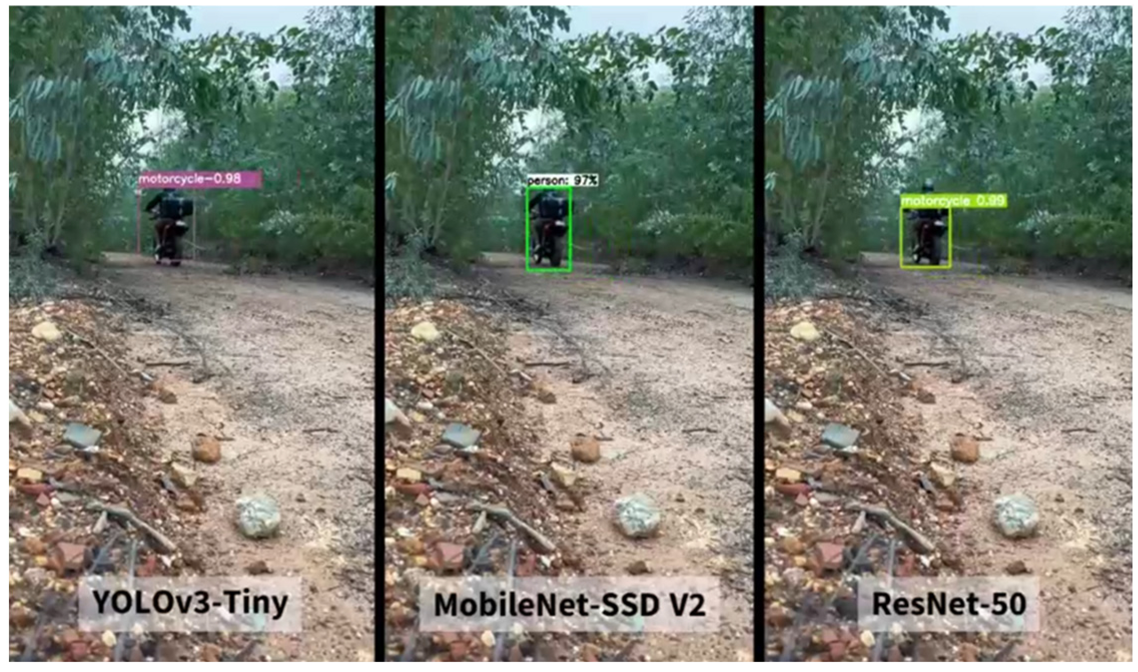
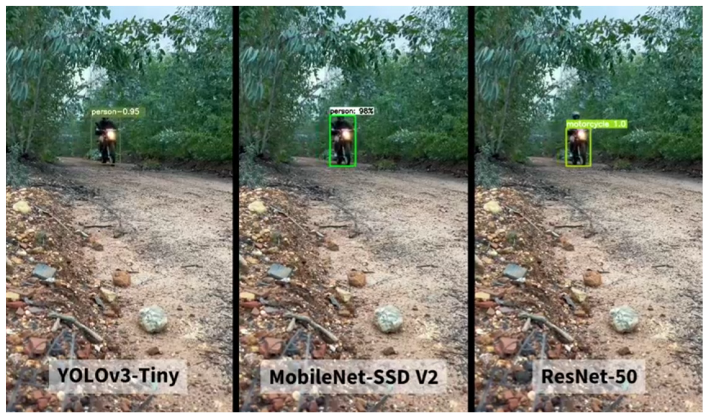
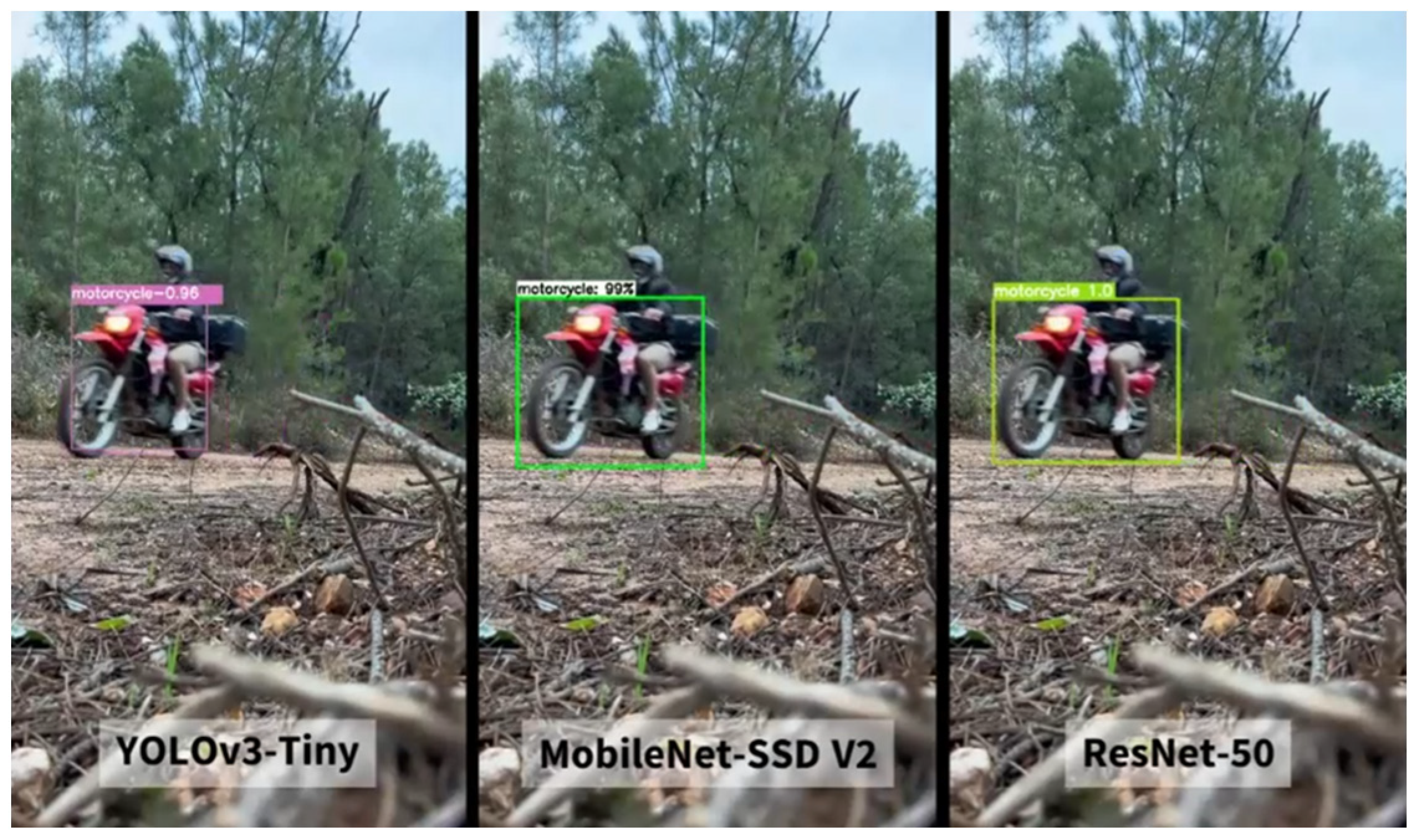
4.4.2. Tests
5. Conclusions
Author Contributions
Funding
Data Availability Statement
Conflicts of Interest
References
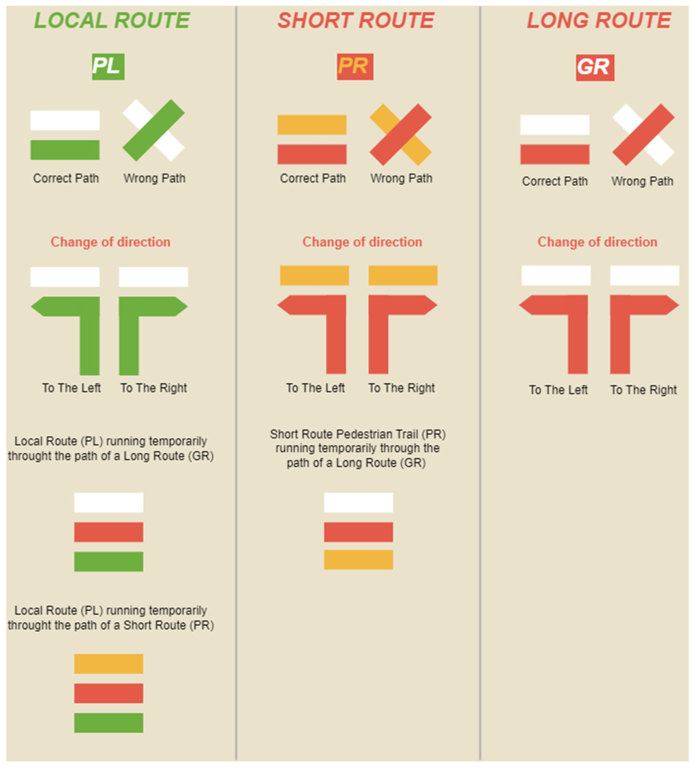
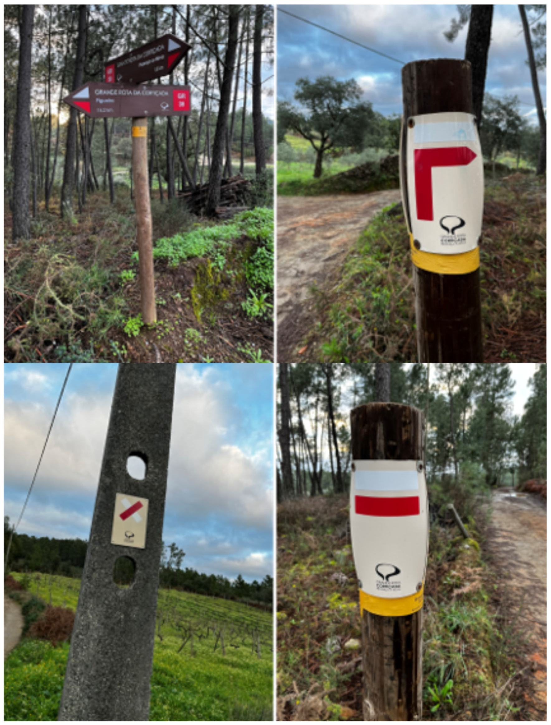
- Federação de Campismo e Montanhismo de Portugal Regulamento de Homologação De Percursos. Lisboa, Portugal, 2006. Available online: https://cm-nisa.pt/images/documentos/areas_atividade/desporto/regulamentopercursospedestres.pdf (accessed on 9 December 2023).
- Sinalização. Available online: http://www.solasrotas.org/2008/09/sinalizao.html (accessed on 9 December 2023).
- Carvalho, P. Pedestrianismo e Percursos Pedestres; Cadernos de Geograia: Coimbra, Portugal, 2009. [Google Scholar]
- Federação de Campismo e Montanhismo de Portugal Site Oficial Da FCMP. Available online: https://www.fcmportugal.com/ (accessed on 16 January 2024).
- Federação de Campismo e Montanhismo de Portugal Site Oficial Da FCMP—Percursos Pedestres. Available online: https://www.fcmportugal.com/percursos-pedestres/ (accessed on 9 December 2023).
- Zhao, W.; Li, J. A Survey of Object Detection Methods in Inclement Weather Conditions. In Proceedings of the 2023 IEEE International Conference on Unmanned Systems (ICUS), Hefei, China, 13–15 October 2023; IEEE: New York, NY, USA, 2023; pp. 1405–1412. [Google Scholar]
- Vavilin, A.; Lomov, A.; Roman, T. Real-Time Train Wagon Counting and Number Recognition Algorithm. In Proceedings of the 2022 International Workshop on Intelligent Systems (IWIS), Ulsan, Republic of Korea, 17–19 August 2022; pp. 1–4. [Google Scholar]
- Gideon Why Vision Is Better than LiDAR. Available online: https://www.gideon.ai/resources/why-is-vision-better-than-lidar-for-logistics-robots/ (accessed on 27 February 2024).
- Cardoso, O. Visão Computacional: Desafios e Avanços Recentes Na Área|Vigeversa. Available online: https://vigeversa.com/inteligencia-artificial/visao-computacional/ (accessed on 27 February 2024).
- Roboflow Inc. Roboflow Website. Available online: https://roboflow.com/ (accessed on 22 November 2023).
- Prisma PRISMA Statement. Available online: http://www.prisma-statement.org/ (accessed on 6 November 2023).
- FCCN Biblioteca Do Conhecimento Online (b-On). Available online: https://www.b-on.pt/ (accessed on 7 November 2023).
- ISCTE, B. Guia de Apoio Ao Utilizador (b-On); Lisboa, Portugal, 2013; Volume 3. Available online: https://www.iscte-iul.pt/assets/files/2017/01/30/1485777979520_Guia_b_on_MOD_SID_AU_003_4.pdf (accessed on 7 November 2023).
- Minh, K.T.; Dinh, Q.-V.; Nguyen, T.-D.; Nhut, T.N. Vehicle Counting on Vietnamese Street. In Proceedings of the 2023 IEEE Statistical Signal Processing Workshop (SSP), Hanoi, Vietnam, 2–5 July 2023; pp. 160–164. [Google Scholar]
- Hong, C.J.; Mazlan, M.H. Development of Automated People Counting System Using Object Detection and Tracking. Int. J. Online Biomed. Eng. 2023, 19, 18–30. [Google Scholar] [CrossRef]
- Chatrasi, A.L.V.S.S.; Batchu, A.G.; Kommareddy, L.S.; Garikipati, J. Pedestrian and Object Detection Using Image Processing by YOLOv3 and YOLOv2. In Proceedings of the 7th International Conference on Trends in Electronics and Informatics, ICOEI 2023—Proceedings, Tirunelveli, India, 11–13 April 2023; pp. 1667–1672. [Google Scholar]
- Anil, J.M.; Mathews, L.; Renji, R.; Jose, R.M.; Thomas, S. Vehicle Counting Based on Convolution Neural Network. In Proceedings of the 7th International Conference on Intelligent Computing and Control Systems, ICICCS, Madurai, India, 17–19 May 2023; pp. 695–699. [Google Scholar]
- Myint, E.P.; Sein, M.M. People Detecting and Counting System. In LifeTech 2021, Proceedings of the 2021 IEEE 3rd Global Conference on Life Sciences and Technologies, Nara, Japan, 9–11 March 2021; IEEE: Nara, Japan, 2021; pp. 289–290. [Google Scholar]
- Kolluri, J.; Das, R. Intelligent Multimodal Pedestrian Detection Using Hybrid Metaheuristic Optimization with Deep Learning Model. Image Vis. Comput. 2023, 131, 104268. [Google Scholar] [CrossRef]
- Mimboro, P.; Heryadi, Y.; Lukas; Suparta, W.; Wibowo, A. Realtime Vehicle Counting Method Using Haar Cascade Classifier Model. In Proceedings of the 2021 International Conference on Advanced Mechatronics, Intelligent Manufacture and Industrial Automation, ICAMIMIA, Surabaya, Indonesia, 8–9 December 2021; IEEE: Surabaya, Indonesia, 2021; pp. 229–233. [Google Scholar]
- Vignarca, D.; Prakash, J.; Vignati, M.; Sabbioni, E. Improved Person Counting Performance Using Kalman Filter Based on Image Detection and Tracking. In Proceedings of the 2021 AEIT International Conference on Electrical and Electronic Technologies for Automotive, AEIT AUTOMOTIVE, Torino, Italy, 17–19 November 2021; IEEE: Torino, Italy, 2021; pp. 1–6. [Google Scholar]
- Minh, H.T.; Mai, L.; Minh, T.V. Performance Evaluation of Deep Learning Models on Embedded Platform for Edge AI-Based Real Time Traffic Tracking and Detecting Applications. In Proceedings of the 2021 15th International Conference on Advanced Computing and Applications, ACOMP, Ho Chi Minh City, Vietnam, 24–26 November 2021; pp. 128–135. [Google Scholar]
- Kim, J.; Suh, Y.; Lee, J.; Chae, H.; Ahn, H.; Chung, Y.; Park, D. EmbeddedPigCount: Pig Counting with Video Object Detection and Tracking on an Embedded Board. Sensors 2022, 22, 2689. [Google Scholar] [CrossRef] [PubMed]
- Gomes, H.; Redinha, N.; Lavado, N.; Mendes, M. Counting People and Bicycles in Real Time Using YOLO on Jetson Nano. Energies 2022, 15, 8816. [Google Scholar] [CrossRef]
- LeCun, Y.; Bengio, Y.; Hinton, G. Deep Learning. Nature 2015, 521, 436–444. [Google Scholar] [CrossRef] [PubMed]
- Morera, Á.; Sánchez, Á.; Moreno, A.B.; Sappa, Á.D.; Vélez, J.F. SSD vs. YOLO for Detection of Outdoor Urban Advertising Panels under Multiple Variabilities. Sensors 2020, 20, 4587. [Google Scholar] [CrossRef] [PubMed]
- Amazon Web Services O Que é Visão Computacional?—Explicação de IA/ML de Reconhecimento de Imagem—AWS. Available online: https://aws.amazon.com/pt/what-is/computer-vision/ (accessed on 30 October 2023).
- IBM O Que São Redes Neurais? IBM. Available online: https://www.ibm.com/br-pt/topics/neural-networks (accessed on 17 October 2023).
- Nunes dos Santos, V. Reconhecimento de Objetos Em Uma Cena Utilizando Redes Neurais Convolucionais. Bachelor’s Thesis, Universidade Tecnológica Federal do Paraná, Curitiba, Brazil, 2018. [Google Scholar]
- Bhatt, D.; Patel, C.; Talsania, H.; Patel, J.; Vaghela, R.; Pandya, S.; Modi, K.; Ghayvat, H. CNN Variants for Computer Vision: History, Architecture, Application, Challenges and Future Scope. Electronics 2021, 10, 2470. [Google Scholar] [CrossRef]
- Deep Learning Book Capítulo 43—Camadas de Pooling Em Redes Neurais Convolucionais. Available online: https://www.deeplearningbook.com.br/camadas-de-pooling-em-redes-neurais-convolucionais/ (accessed on 5 November 2023).
- Barbosa, G.; Bezerra, G.M.; de Medeiros, D.S.; Andreoni Lopez, M.; Mattos, D. Segurança Em Redes 5G: Oportunidades e Desafios Em Detecção de Anomalias e Predição de Tráfego Baseadas Em Aprendizado de Máquina. In Proceedings of the Minicursos do XXI Simpósio Brasileiro de Segurança da Informação e de Sistemas Computacionais, Online, Belém, 4–7 October 2021; pp. 164–165. [Google Scholar] [CrossRef]
- Poloni, K. Redes Neurais Convolucionais. Available online: https://medium.com/itau-data/redes-neurais-convolucionais-2206a089c715 (accessed on 1 November 2023).
- Archana, V.; Kalaiselvi, S.; Thamaraiselvi, D.; Gomathi, V.; Sowmiya, R. A Novel Object Detection Framework Using Convolutional Neural Networks (CNN) and RetinaNet. In Proceedings of the International Conference on Automation, Computing and Renewable Systems, ICACRS, Pudukkottai, India, 13–15 December 2022; pp. 1070–1074. [Google Scholar]
- Carranza-García, M.; Torres-Mateo, J.; Lara-Benítez, P.; García-Gutiérrez, J. On the Performance of One-Stage and Two-Stage Object Detectors in Autonomous Vehicles Using Camera Data. Remote Sens. 2020, 13, 89. [Google Scholar] [CrossRef]
- Zhou, L.; Lin, T.; Knoll, A. Fast and Accurate Object Detection on Asymmetrical Receptive Field. Comput. Vis. Pattern Recognit. Arxiv 2023, arXiv:2303.08995. [Google Scholar] [CrossRef]
- Thakur, N. A Detailed Introduction to Two Stage Object Detectors. Available online: https://namrata-thakur893.medium.com/a-detailed-introduction-to-two-stage-object-detectors-d4ba0c06b14e (accessed on 23 December 2023).
- Redmon, J.; Farhadi, A. YOLOv3: An Incremental Improvement. Comput. Vis. Pattern Recognit. 2018, arXiv:1804.02767. [Google Scholar] [CrossRef]
- Bajaj, V. The YOLO Algorithm—Deep Learning Specialization—Coursera. Available online: https://vikram-bajaj.gitbook.io/deep-learning-specialization-coursera/convolutional-neural-networks/object-detection/the-yolo-algorithm (accessed on 28 January 2024).
- Adarsh, P.; Rathi, P.; Kumar, M. YOLO V3-Tiny: Object Detection and Recognition Using Stage Improved Model. In Proceedings of the 2020 6th International Conference on Advanced Computing & Communication Systems (ICACCS), Coimbatore, India, 6–7 March 2020; pp. 687–694. [Google Scholar]
- Li, T.; Ma, Y.; Endoh, T. A Systematic Study of Tiny YOLO3 Inference: Toward Compact Brainware Processor With Less Memory and Logic Gate. IEEE Access 2020, 8, 142931–142955. [Google Scholar] [CrossRef]
- Cochard, D. MobilenetSSD: A Machine Learning Model for Fast Object Detection. Available online: https://medium.com/axinc-ai/mobilenetssd-a-machine-learning-model-for-fast-object-detection-37352ce6da7d (accessed on 16 January 2024).
- Sabina, N.; Aneesa, M.P.; Haseena, P.V. Object Detection Using YOLO And Mobilenet SSD: A Comparative Study. Int. J. Eng. Res. Technol. 2022, 11, 136–138. [Google Scholar]
- Howard, A.; Sandler, M.; Chu, G.; Chen, L.-C.; Chen, B.; Tan, M.; Wang, W.; Zhu, Y.; Pang, R.; Vasudevan, V.; et al. Searching for MobileNetV3. Comput. Vis. Pattern Recognit. 2019, arXiv:1905.02244. [Google Scholar] [CrossRef]
- Sovit Rath, R. Object Detection Using PyTorch Faster RCNN ResNet50 FPN V2. Available online: https://debuggercafe.com/object-detection-using-pytorch-faster-rcnn-resnet50-fpn-v2/ (accessed on 26 February 2024).
- ResNet-50: The Basics and a Quick Tutorial. Available online: https://datagen.tech/guides/computer-vision/resnet-50/ (accessed on 26 February 2024).
- Ren, S.; He, K.; Girshick, R.; Sun, J. Faster R-CNN: Towards Real-Time Object Detection with Region Proposal Networks. IEEE Trans. Pattern Anal. Mach. Intell. 2017, 39, 1137–1149. [Google Scholar] [CrossRef] [PubMed]
- Pixabay Pixabay Website. Available online: https://pixabay.com/ (accessed on 29 November 2023).
- Unsplash Unsplash Website. Available online: https://unsplash.com/pt-br (accessed on 29 November 2023).
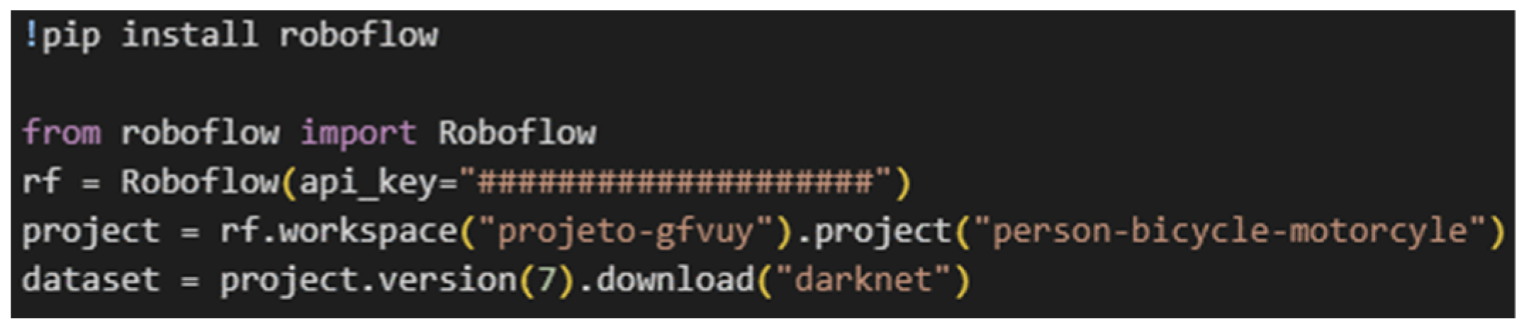
- Miguel, J.; Mendonça, P. Person, Bicycle and Motorcyle Dataset. Available online: https://universe.roboflow.com/projeto-gfvuy/person-bicycle-motorcyle/model/7 (accessed on 26 January 2024).
- Nelson, J. How to Label Image Data for Computer Vision Models. Available online: https://blog.roboflow.com/tips-for-how-to-label-images/ (accessed on 15 January 2024).
- Google Colab. Available online: https://colab.google/ (accessed on 22 December 2023).
- Weka Why GPUs for Machine Learning? A Complete Explanation—WEKA. Available online: https://www.weka.io/learn/ai-ml/gpus-for-machine-learning/ (accessed on 23 December 2023).
- Google Colab—FAQ. Available online: https://research.google.com/colaboratory/faq.html#resource-limits (accessed on 15 January 2024).
- Armazenamento Na Nuvem Pessoal e Plataforma de Partilha de Ficheiros—Google. Available online: https://www.google.com/intl/pt-PT/drive/ (accessed on 23 December 2023).
- Roboflow Notebook—Train Yolov4 Tiny Object Detection On Custom Data. Available online: https://github.com/roboflow/notebooks/blob/main/notebooks/train-yolov4-tiny-object-detection-on-custom-data.ipynb (accessed on 23 December 2023).
- NVIDIA. NVIDIA CUDA Compiler Driver. Available online: https://docs.nvidia.com/cuda/cuda-compiler-driver-nvcc/index.html (accessed on 23 December 2023).
- Darknet Darknet: Open Source Neural Networks in C. Available online: https://pjreddie.com/darknet/ (accessed on 23 December 2023).
- yaming116 Darknet—Yolov3-Tiny Weights. Available online: https://github.com/smarthomefans/darknet-test/blob/master/yolov3-tiny.weights (accessed on 23 December 2023).
- Traore, M. Roboflow’s Python Pip Package For Computer Vision. Available online: https://blog.roboflow.com/pip-install-roboflow/ (accessed on 23 December 2023).
- Charette, S. Programming Comments—Darknet FAQ. Available online: https://www.ccoderun.ca/programming/darknet_faq/ (accessed on 28 January 2024).
- Juras, E.; Technology Consultants, E. Notebook—Train TFLite2 Object Detection Model. Available online: https://colab.research.google.com/github/EdjeElectronics/TensorFlow-Lite-Object-Detection-on-Android-and-Raspberry-Pi/blob/master/Train_TFLite2_Object_Detction_Model.ipynb (accessed on 15 January 2024).
- Juras, E.; Technology Consultants, E.; Miguel, J.; Mendonça, P. Notebook Adaptado—Train TFLite2 Object Detection Model. Available online: https://colab.research.google.com/drive/1rK3GNbJA_i_rupahuWyWgvrEHHvvp44i?authuser=1#scrollTo=fF8ysCfYKgTP (accessed on 15 January 2024).
- TensorFlow; vighneshbirodkar; TF Object Detection Team TensorFlow 2 Detection Model Zoo. Available online: https://github.com/tensorflow/models/blob/master/research/object_detection/g3doc/tf2_detection_zoo.md (accessed on 15 January 2024).
- sovit-123 FasterRCNN Pytorch Training Pipeline: PyTorch Faster R-CNN Object Detection on Custom Dataset. Available online: https://github.com/sovit-123/fasterrcnn-pytorch-training-pipeline (accessed on 15 January 2024).
- PyTorch PyTorch. Available online: https://pytorch.org/ (accessed on 24 December 2023).
- Lakera Average Precision. Available online: https://www.lakera.ai/ml-glossary/average-precision (accessed on 17 January 2024).
- Cook, J.A.; Ranstam, J. Overfitting. Br. J. Surg. 2016, 103, 1814. [Google Scholar] [CrossRef] [PubMed]
- Ying, X. An Overview of Overfitting and Its Solutions. J. Phys. Conf. Ser. 2019, 1168, 022022. [Google Scholar] [CrossRef]
- TensorFlow TensorBoard. Available online: https://www.tensorflow.org/tensorboard?hl=pt-br (accessed on 16 January 2024).
- Rosebrock, A. YOLO and Tiny-YOLO Object Detection on the Raspberry Pi and Movidius NCS—PyImageSearch. Available online: https://pyimagesearch.com/2020/01/27/yolo-and-tiny-yolo-object-detection-on-the-raspberry-pi-and-movidius-ncs/ (accessed on 17 January 2024).
- Serra, R. Como Funcionam Os Painéis Solares Para Casa? Available online: https://www.doutorfinancas.pt/energia/como-funcionam-os-paineis-solares-para-casa/ (accessed on 29 November 2023).


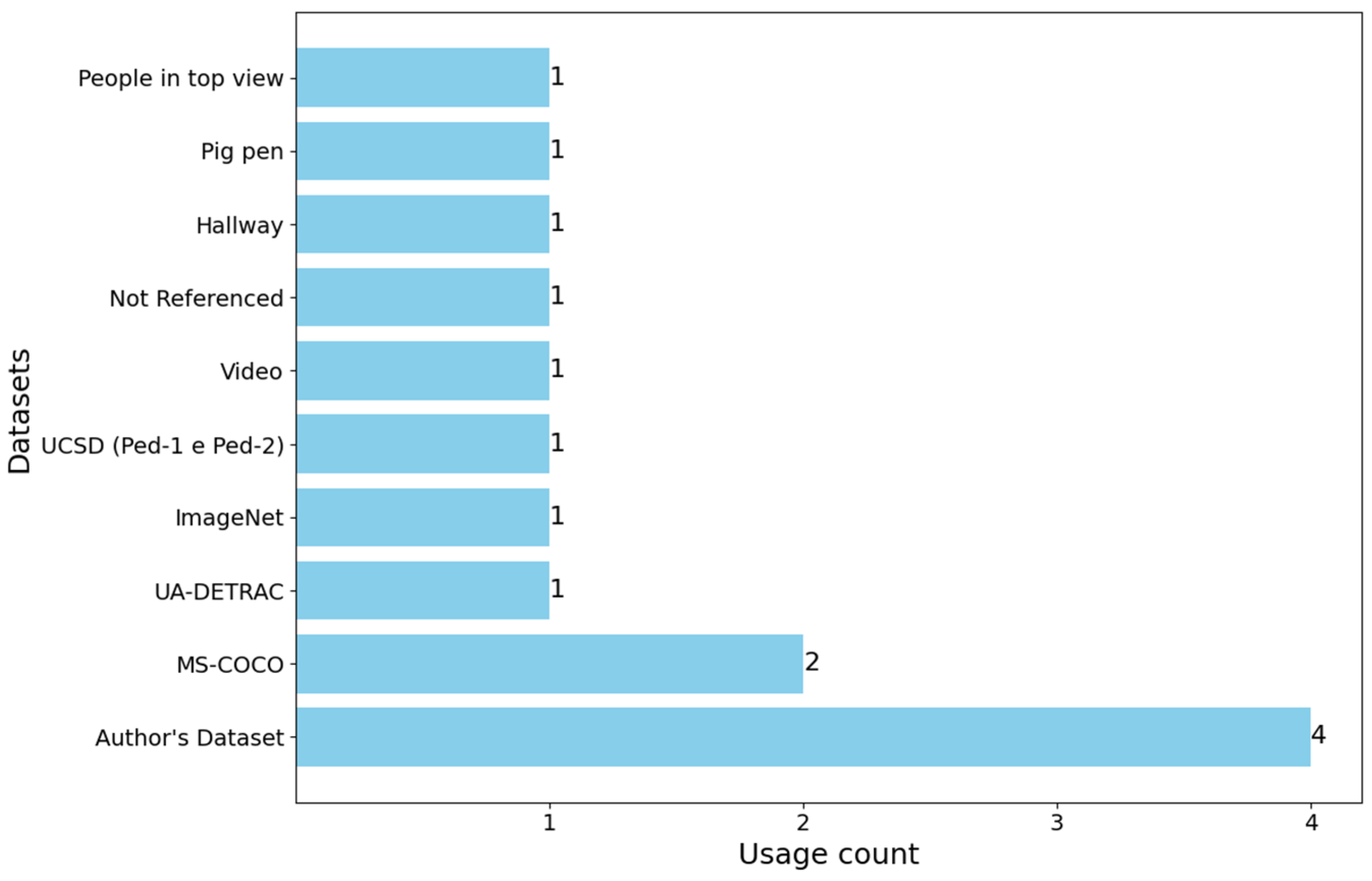
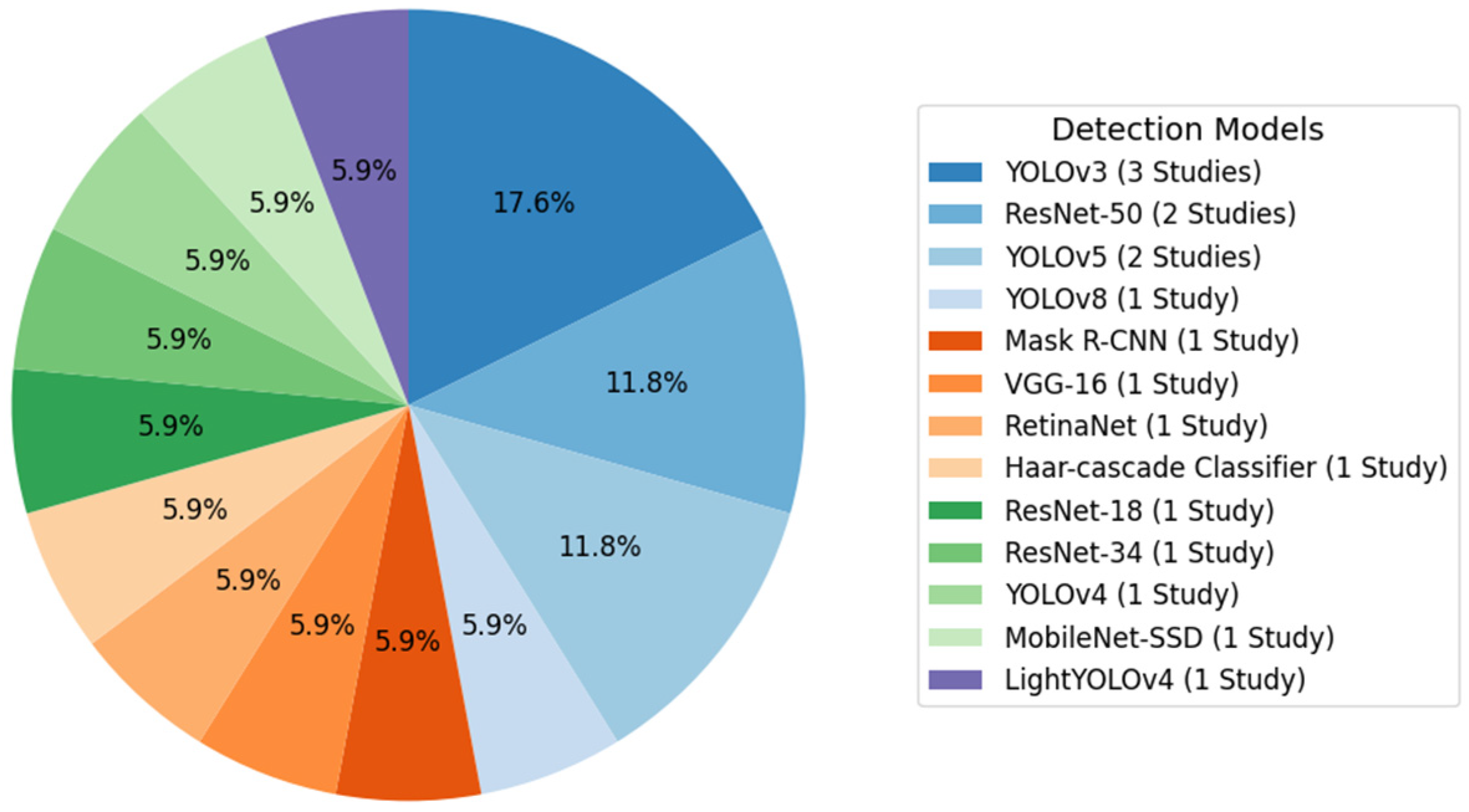
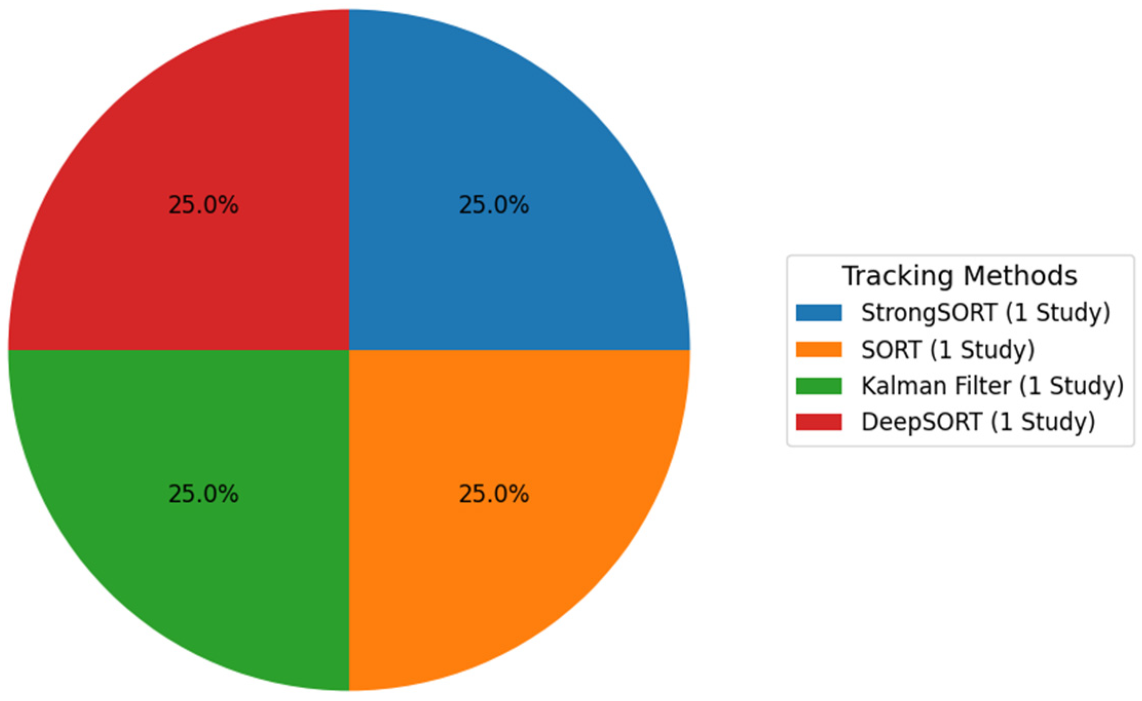
| References | Study | Year | Dataset | Methodologies | Results |
|---|---|---|---|---|---|
| [14] | Vehicle Counting on Vietnamese Street | 2023 | Dataset created by the author | YOLOv8, StrongSORT | mAP of 82.9% |
| [15] | Development of Automated People Counting System using Object Detection and Tracking | 2023 | MS-COCO | Mask R-CNN, ResNet-50 | mAP of 100% and 97.62% in plans with simple funds and 85.73% in complex funds |
| [16] | Pedestrian and Object Detection using Image Processing by YOLOv3 and YOLOv2 | 2023 | MS-COCO | YOLOv3 | mAP of 57.9% |
| [17] | Vehicle Counting based on Convolution NeuralNetwork | 2023 | UA-DETRAC | YOLOv3, SORT | Counting accuracy of 85.45% |
| [18] | People Detecting and Counting System | 2021 | ImageNet | ImageNet | N/A |
| [19] | Intelligent multimodal pedestrian detection using hybrid metaheuristic optimization with deep learning model | 2023 | UCSD (Ped-1 e Ped-2) | YOLO-v5, RetinaNet | AUC score of 98.86% (Ped-1) and 97.58% (Ped-2) |
| [20] | Realtime Vehicle Counting Method Using Haar Cascade Classifier Model | 2021 | 3 min video (origin not described) | Haar Cascade Classifier algorithm | mAP of 91.2% |
| [7] | Real-time Train Wagon Counting and Number Recognition Algorithm | 2022 | Dataset created by the authors | ResNet-18, ResNet-34, ResNet-50 | Accuracy of 99.2% at 36 FPS (ResNet-18), 99.4% at 22 FPS (ResNet-34), and 99.7% at 10 FPS (ResNet-50) |
| [21] | Improved Person Counting Performance Using Kalman Filter Based on Image Detection and Tracking | 2021 | N/A | YOLOv3 e Kalman Filter | N/A |
| [22] | Performance Evaluation of Deep Learning Models on Embedded Platform | 2021 | Dataset created by the authors | YOLOv4, MobileNet-SSD | mAP of 91% with 7.2 FPS (YOLOv4) and 87.5% with 40 FPS (MobileNet-SSD) |
| [23] | EmbeddedPigCount: Pig Counting with Video Object Detection and Tracking on an Embedded Board | 2022 | Hallway, pig pen, people in top view | LightYOLOv4, DeepSORT | mAP of 94.95% |
| [24] | Counting People and Bicycles in Real Time Using YOLO on Jetson Nano | 2022 | Dataset created by the authors | Yolov5, V-IOU | mAP of 44.4% |
| No. of Training Images | No. of Validation Images | No. of Test Images | |
|---|---|---|---|
| Persons | 180 | 53 | 25 |
| Bicycles | 63 | 17 | 9 |
| Motorcycles | 68 | 19 | 8 |
| Total | 311 | 89 | 42 |
| AP | mAP | FPS | |
|---|---|---|---|
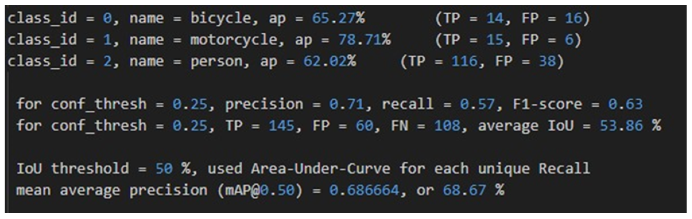
| YOLOv3-Tiny | Bicycle: 65.27% Motorcycle: 78.71% Person: 62.02% | 68.7% | 16.58 |
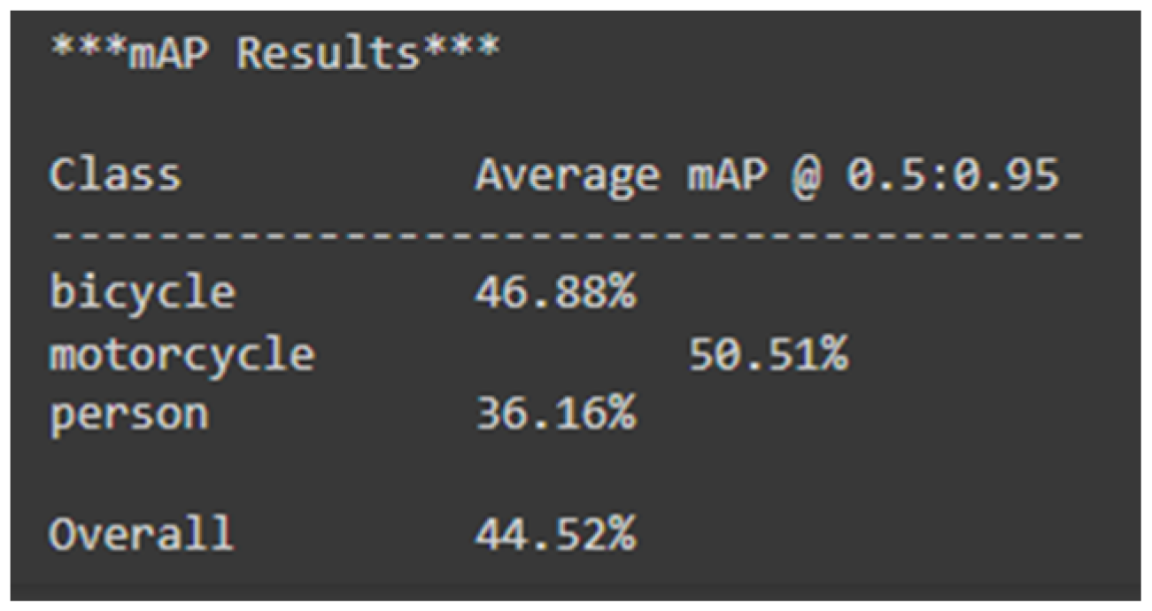
| MobileNet-SSD V2 | Bicycle: 46.88% Motorcycle: 50.51% Person: 36.16% | 44.52% | 27.85 |
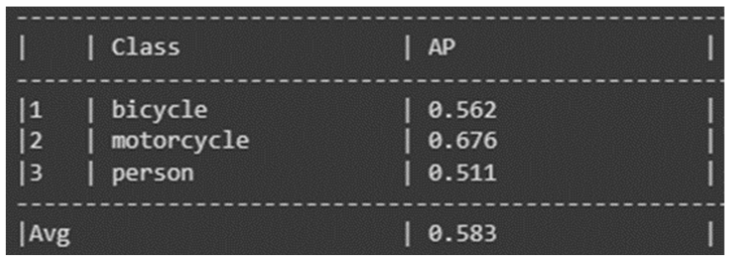
| FasterRCNN and ResNet-50 | Bicycle: 56.2% Motorcycle: 67.6% Person: 51.1% | 58.3% | 4.15 |
Disclaimer/Publisher’s Note: The statements, opinions and data contained in all publications are solely those of the individual author(s) and contributor(s) and not of MDPI and/or the editor(s). MDPI and/or the editor(s) disclaim responsibility for any injury to people or property resulting from any ideas, methods, instructions or products referred to in the content. |
© 2024 by the authors. Licensee MDPI, Basel, Switzerland. This article is an open access article distributed under the terms and conditions of the Creative Commons Attribution (CC BY) license (https://creativecommons.org/licenses/by/4.0/).
Share and Cite
Miguel, J.; Mendonça, P.; Quelhas, A.; Caldeira, J.M.L.P.; Soares, V.N.G.J. Using Computer Vision to Collect Information on Cycling and Hiking Trails Users. Future Internet 2024, 16, 104. https://doi.org/10.3390/fi16030104
Miguel J, Mendonça P, Quelhas A, Caldeira JMLP, Soares VNGJ. Using Computer Vision to Collect Information on Cycling and Hiking Trails Users. Future Internet. 2024; 16(3):104. https://doi.org/10.3390/fi16030104
Chicago/Turabian StyleMiguel, Joaquim, Pedro Mendonça, Agnelo Quelhas, João M. L. P. Caldeira, and Vasco N. G. J. Soares. 2024. "Using Computer Vision to Collect Information on Cycling and Hiking Trails Users" Future Internet 16, no. 3: 104. https://doi.org/10.3390/fi16030104