Forecasting Monthly Prices of Japanese Logs

Abstract

Forecasts of prices can help industries in their risk management. This is especially true for Japanese logs, which experience sharp fluctuations in price. In this research, the authors used an exponential smoothing method (ETS) and autoregressive integrated moving average (ARIMA) models to forecast the monthly prices of domestic logs of three of the most important species in Japan: sugi (Japanese cedar, Cryptomeria japonica D. Don), hinoki (Japanese cypress, Chamaecyparis obtusa (Sieb. et Zucc.) Endl.), and karamatsu (Japanese larch, Larix kaempferi (Lamb.) Carr.). For the 12-month forecasting periods, forecasting intervals of 80% and 95% were given. By measuring the accuracy of forecasts of 12- and 6-month forecasting periods, it was found that ARIMA gave better results than did the ETS in the majority of cases. However, the combined method of averaging ETS and ARIMA forecasts gave the best results for hinoki in several cases.

1. Introduction

Fluctuations and low levels of log prices in Japan are a challenge for forest owners in managing forests. As a result, processing mills experience difficulties in ensuring a stable supply of suitable logs. Additionally, the mismatch between the supply of and demand for logs leads to sharp fluctuations in log prices, such as that observed in the former half of 2012 [1]. In other words, log prices not only affect the profitability of forest owners, logging companies and sawmills, but might also affect the daily operations in sawmills. Therefore, having information on future log prices can be useful for the aforementioned parties in their risk management. For example, information about potential price fluctuations will perhaps allow suppliers and users of logs to adjust their supply and demand. When private suppliers of logs feel it is difficult to adjust their supplies due to small size of their operations and the need to cover daily maintenance costs, state-owned forests managers might play an important role by adjusting their supplies of logs. However, forecasts of log prices in Japan have rarely been provided, though analyses on fluctuations in the prices of Japanese logs started long ago.

The impacts of various supply and demand factors on log prices have been studied and the existence of seasonal fluctuations confirmed as early as in the late 1920s [2]. Log prices are found to be at their lowest in June and July and to reach their peak in October and November due to the seasonal nature of construction (spring and autumn were peak times), but, in 1910–1920’s, seasonal fluctuations have become less pronounced, about 1% of the annual average prices [2]. Recently, a monthly seasonal price index for logs of different origins (e.g., Mainland Japan, North America, Hokkaido, South Asia, and Taiwan) in Tokyo and Osaka markets has been calculated [3], but, in response to this research, it was noted that the seasonal increase in autumn is rather limited and should not be expected, because the general commodity market is thought to be more important [4]. Since the 1960s, not only the seasonal fluctuations, but the trend movement in log prices with the changes in supply and demand has also been analyzed [5,6,7,8]. The cyclical fluctuations and their relationship with the diffusion index, apart from demand and supply, have also attracted the attention of researchers [9]. The number of months from one valley to the next valley were calculated to show the cycles of timber prices [9]. In the 1980s, a decomposition method, which was developed by Economic Planning Agency, Japan, originating from the Census Method II approach (US Census Bureau), was used in analyzing the trend, cycle, and seasonal movements for log price time series along with their influencing factors [10]. In the 2000s, the X-12-ARIMA approach, developed by U.S. Census Bureau and mainly used for seasonal adjustment, was adopted to decompose the price time series into trend components, seasonal components, and irregular components for nine forest products in two private auction markets in the Kyushu region [11]. A recent study in the field analyzed the relationship between monthly prices and log inventory in sawmills and stated that pest damage is the reason for low prices from June to August [12]. Although the aforementioned research studies paid attention to price fluctuations, few forecasts could be found among them. In the 1970s, a two-step foresting approach was once adopted in which the price time series was decomposed into the following components: secular trend variation, which is determined by stock supply; seasonal variation, which is caused by the seasonal change in activities in construction; cyclical fluctuation, which is largely caused by business cycle; and random variation, which is fitted into an AR mode. These components were then combined together using the models established in the above stages for forecasting. As for the forecasting period, two years of monthly forecasts were provided, as were the lower and upper limits of forecasts at the 70% level, but the methods used to calculate these lower and upper limits were not explained [7]. Moving average (MA), autoregressive moving average (ARMA), and seasonal autoregressive integrated moving average (ARIMA) models were once used for fitting price time series of some sawnwood and logs, and it was concluded that the most reasonable forecast results were obtained by using the seasonal ARIMA [11], even though only a simple form of the ARIMA model was considered.

Short-term forecasting of a time series is possible because each time series has its own pattern of movements. To do a forecast well, a good grasp of the situation is important, and forecasters need to make subjective judgments at times. Therefore, statistical forecasting can be described as “the blend of art and science” [13], and the objective of time series forecasting is “to discover the pattern in the historical data series and extrapolate that pattern into the future” [14]. More complicated models are not considered in this research because model simplicity is preferred, though exponential smoothing method (ETS) and ARIMA have evolved into complicated forms already.

ETS and ARIMA have made great progress since the 1990s [14,15]. The free software R [16] and the package forecast [17] make specifying parameters and comparing models much easier. ETS’s model framework has made progress by introducing the state space model as well as other developments, such as stochastic models, likelihood calculation, prediction intervals, and procedures for model selection [15].

In this research, by applying the latest model specification and selection instruments and the algorithm in software R (R Core Team, Vienna, Austria), we analyze the movements in prices of domestic Japanese sawlogs—sugi, hinoki, and karamatsu. We then forecast log prices 12 months ahead by using ETS and ARIMA. In addition to point forecasts, we give forecast intervals at the 80% and 95% levels. Additionally, we apply valuations for forecast accuracy to forecast results given by ETS and ARIMA and concluded that, in most cases, ARIMA obtains better forecasts than ETS does.

2. Materials and Methods

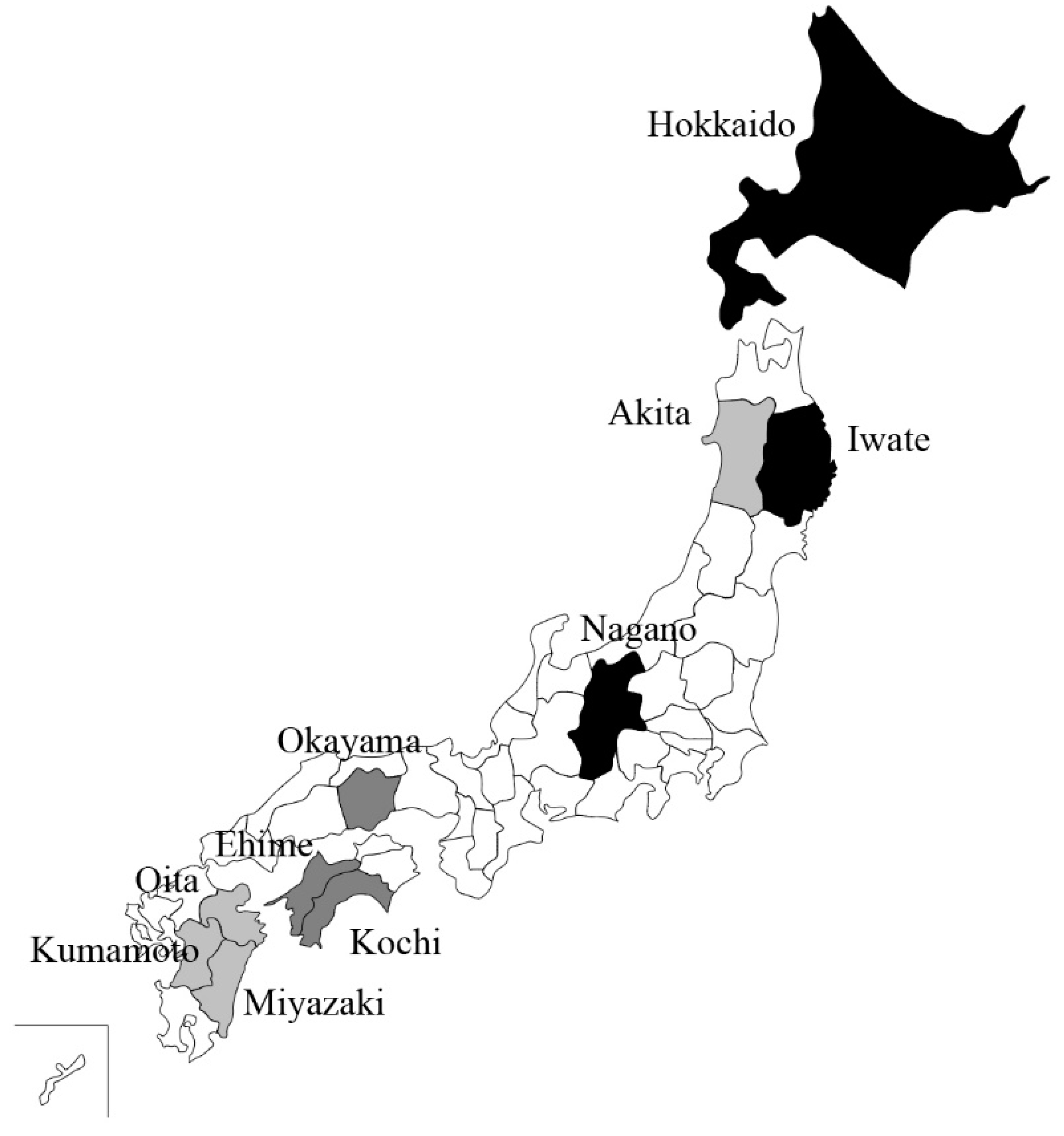
2.1. Study Objects and Their Data

Forests in Japan cover about 67% of the total area and, due to aggressive planting since 1950s, the area of planted forests in Japan extends to over 10 million ha, which is 40% of the total forest area. Due to the low level of harvest volume compared to the growth level, the total forest stock keeps increasing, and the average growing stock per hectare comes to over 190 m³ [18]. In Japan, most forest owners and sawmills are small in scale. It is difficult for small owners to provide a steady supply of logs, and it is difficult for small mills to produce kiln-dried sawnwood to compete against foreign sawnwood. Increasing costs, which are partly driven by increasing wages, are another factor for the low competitiveness of domestic logs and sawnwood. The production of logs declined to 15 million m³ by 2002 from 51 million m³ in 1967, when Japan opened the door to foreign timber products. After the efforts of the Japanese government and wood industry to promote domestic wood, the self-sufficiency rate of wood recovered from its lowest point of 18.2% in 2002 to 31.2% in 2014 [19].

The top three species for log production in Japan—sugi, hinoki, and karamatsu—are mainly harvested from the planted forests. In 2014, the production volumes for these three species are 11.19 million m³ (56% of the total log production), 2.40 million m³ (12%), and 2.37 million m³ (12%), respectively [20]. The main prefectures for sugi production are Miyazaki, Akita, Oita, and Kumamoto; the top producers for hinoki are Okayama, Kochi, Ehime, and Kumamoto; and for karamatsu, they are Hokkaido, Iwate, and Nagano (see Figure 1). Sugi and hinoki sawnwood are mainly used in housing construction, and karamatsu sawnwood is mainly used as packaging materials for the storage and transportation of commodities.

Logs of different diameters and lengths might have different usages, which translates into different prices. In this research, we analyze sugi, hinoki, and karamatsu logs in their most common diameters and lengths for sawnwood processing. For sugi and hinoki, the diameter is 14–22 cm, for karamatsu, it is 14–28 cm; the length considered for the logs of the three species is 3.65–4.00 m [20]. The prices are monthly volume-weighted average prices for all grades of logs that are used in processing sawnwood under the above-stated diameters and lengths. Our objective is to provide short-term forecasts; thus, considering the data availability, we think that monthly data are suitable.

Given that 2002 was the year when domestic log production decreased to its lowest point since 1960 and subsequently increased, monthly data from January 2002 to September 2015 are used in this research. The current value for monthly prices for logs was sourced from the Ministry of Agriculture, Forestry and Fisheries (MAFF) [20]. Japan experienced deflation after the mid-1990s. However, the situation has changed since 2012, when Abenomics policies began to be implemented. Considering the possible impacts of general price level changes on the movements in log prices, we introduced the Corporate Goods Price Index (CGP) to adjust the monthly log prices to a constant value as that in 2010.

2.2. Methods

In the short-term forecasting of monthly prices of logs, we applied ETS and ARIMA, two typical forecasting approaches, though many methods have been proposed and applied in the field [14,21,22,23,24,25,26,27], and there are “as many forecasting methods as there are forecasters” [28]. Further, the naïve (or seasonal naïve, shortened as Snaïve) method was also introduced as a reference for measuring the accuracy of forecasting. Because we only used the time series data of monthly log prices and no other variables were included (e.g., housing starts on the demand side, forest resources on the supply side), our research is a univariate time series analysis. Root mean square error (RMSE), mean absolute error (MAE) and mean absolute percentage error (MAPE) are calculated in measuring the accuracy of forecasting results.

2.2.1. Naïve Method and Snaïve Method

Company managers or business people occasionally use simple methods to forecast, and these methods can be useful. Using the average value (the mean) of historical data might be useful for time series that fluctuate around some constant value. For a random walk time series, without any trend and seasonality, a naïve method might be useful in which the most recent observation is taken as a forecast for the next period or periods. For a seasonal time series, a Snaïve method might be useful; by which the actual value in the same period of the previous year is taken as a forecast for that period in this year. In measuring the accuracy of forecasting, the naïve or seasonal Snaïve method was used as a reference for that of ETS and ARIMA, because we think that ETS and ARIMA at least should make forecasts with errors as small as naïve or Snaïve method.

2.2.2. ETS

The ETS forecasting approach was proposed in the 1950s and used in inventory control [29,30,31]. The simple ETS has the following form:

$${\widehat{y}}_{t+1|t}={\widehat{y}}_{t|t-1}+\alpha (y_t-{\widehat{y}}_{t|t-1}), \mathrm{or} {\widehat{y}}_{t+1|t}=\alpha y_t+(1-\alpha ){\widehat{y}}_{t|t-1}$$

(1)

where $y_t$ is a time series, ${\widehat{y}}_{t|t-1}$ is the forecast value for $y_t$ by taking account of all previous values, $y_1$, $y_2$,…, $y_{t-1}$, and $\alpha$ is a smoothing parameter between 0 and 1. For longer-range forecasting by the simple ETS, the forecast formula could be written as ${\widehat{y}}_{t+h|t}={\widehat{y}}_{t+1|t}$, h = 2, 3,…, where h means h periods ahead [15,32].

The most suitable method for a specific time series varies with trend and seasonality. The trend component includes five possibilities: None (N), Additive (A), Additive damped (Ad), Multiplicative (M), and Multiplicative damped (Md). The seasonal component includes three possibilities: None (N), Additive (A), and Multiplicative (M). By combining the trend and seasonal components, in total, this results in 15 methods. If considering additive and multiplicative error terms, there will be 30 methods. The formulae for recursive calculations and point forecasts have been well summarized and can be accessed openly [32]. The package forest in R was used in applying exponential smoothing to the three time series, and AIC (Akaike’s Information Criterion) corrected, AICc, which is appropriate for small sample bias, was adopted for model selection [32,33]. Finally, the best method was chosen by the lowest AICc value.

2.2.3. ARIMA

A time series is weakly stationary if neither the mean nor the autocovariances depend on the time t [34]. Economic time series, such as log price, are usually not stationary because the mean and autocovariances sometimes vary with time t. When differencing the time series, the resulting time series, which represents the changes in the series, is usually stationary. The original time series is called a unit root process in this case. ARIMA can be used to describe these types of time series. By adding the seasonality, a general form for ARIMA can be described as ARIMA (p, d, q) (P, D, Q)_m, where (p, d, q) is the non-seasonal part of the model; (P, D, Q) is the seasonal part; p and P are orders of AR (autoregressive part); d and D are the degrees of first differencing; q and Q are orders of MA (moving average part); and m is the number of periods in a year. For monthly prices, m is 12 [14,32].

In this research, we first confirmed the situations of autocorrelation and partial autocorrelation in the time series, which was helpful in choosing the order of AR and MA. Then, we tested stationarity and determined the meaningful degrees of first differencing. We tried the possible orders of AR and MA and degree of integration. The best ARIMA models were selected according to their AICc statistics. However, we stopped at one degree of differencing the time series. Differencing twice makes it difficult to explain the economic meaning of the time series and leads to wider forecasting intervals. The unit root test was implemented to examine the stationarity of both the original time series and the differenced time series. Finally, a diagnostic check of the residuals in ARIMA models was conducted to justify model estimations.

2.2.4. Forecasting Intervals

In addition to point forecasts, we need to present forecasting or prediction intervals to show the range of values within which we believe the actual values to fall with some level of probability. Forecasting intervals show the extent of variability and uncertainty, which can be calculated from variances. Under the Gaussian model assumption, the errors are Gaussian and 100 × (1 − α)% forecasting intervals can be calculated by:

$${\mu }_{n+h|n}\pm z_{\alpha /2}\sqrt{va{r}_{n+h|n}}$$

(2)

where $\mu$ is the forecast mean or point forecast at h periods ahead; $z_{\alpha /2}$ is the $\alpha /2$ significant point in a Gaussian distribution; and var is variance [15]. As shown in statistics textbooks, when the probability level is 0.95, z would be 1.960; when the probability level is 0.80, z would be 1.282.

Forecasting intervals become wider when the forecast periods increase because uncertainty increases with time. Error term will not affect the point forecasts because its expectation value is zero, but it plays an important role in calculating variances and forecasting intervals.

2.2.5. Measures of Forecasting Accuracy

Forecast error is generally defined as $e_t=y_t-{\widehat{y}}_t$, or the difference between the observation and the forecast at time t. This definition is good for one-step forecast. In the case of h-periods-ahead forecasts, ${\widehat{y}}_{t+1}$, ${\widehat{y}}_{t+2}$, …, ${\widehat{y}}_{t+h}$, it is meaningless if $e_t$ is summed because positive and negative errors cancel each other out. Thus, a proper summation of the errors is needed. In our research, three accuracy measures were calculated: RMSE, MAE, and MAPE. The former two are scale-dependent measures, and the last is a percentage point error. Of course, smaller measurement values show more accurate forecasts.

The formulae of these measures are as follows:

$$\mathrm{RMSE}=\sqrt{mean(e_t^2)}; \mathrm{MAE}=\mathrm{mean}(|e_t|); \mathrm{MAPE}=\mathrm{mean}(|100e_t/y_t|)$$

(3)

3. Results

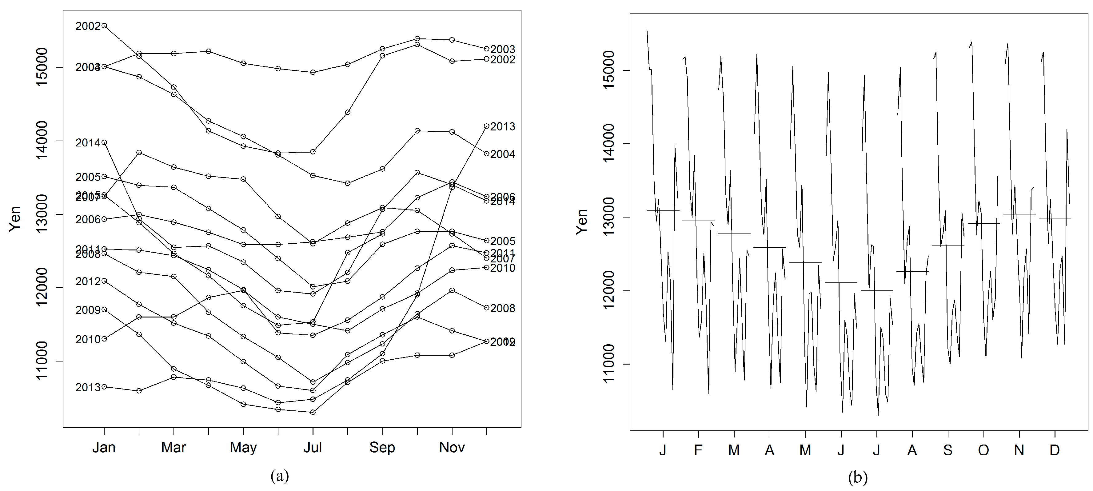
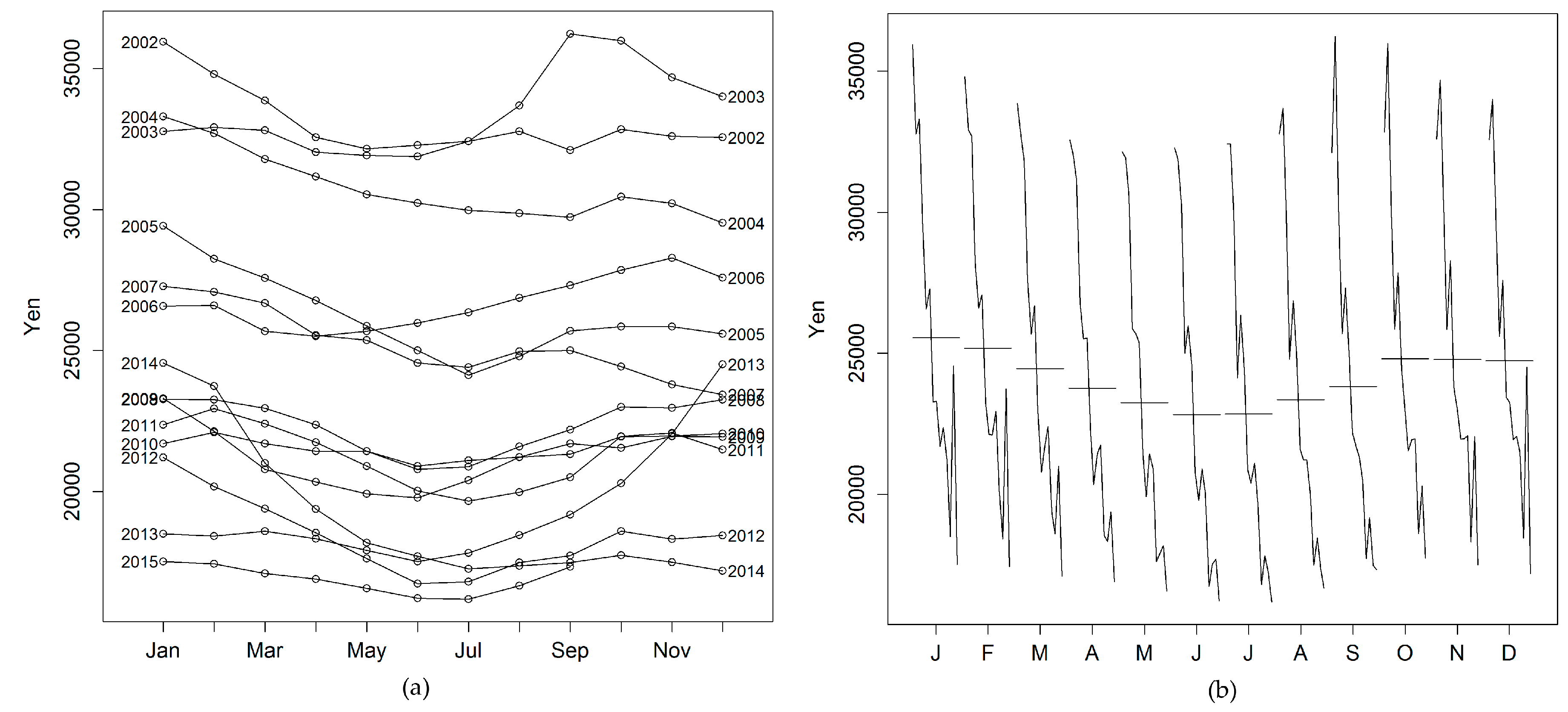
3.1. Seasonal Characteristics

Seasonality in a time series reflects a pattern of ups and downs over a fixed period of time. In Japan, different regions have different climate characteristics, and each region could have its own pattern. The pattern would also affect logging, sawmilling, and the demand for sawnwood, such as demand due to seasonal wood house construction. In the summer season in southern Japan, it is hot and heavy rain can make logging difficult, can damage the road for transportation, and affect the harvest volume. In Northern Japan, rain can be a problem in summer, but in winter, heavy snow leads to lower logging productivity. This pattern of impacts stemming from changes in weather conditions might lead to a seasonal movement in prices for logs. According to industry experts, however, seasonal price fluctuations are most affected by the presence of pests, which damage the quality of logs. Therefore, sawmills try to adjust their log stock and control their acquisition of new logs in spring and summer to avoid or lessen pest damage. Therefore, log prices are low in summer but increase starting from autumn. In contrast, abnormal weather conditions such as extremely heavy snow or rainfall or typhoons affect supply and, thus, prices. When abnormal weather conditions occur, prices will also change due to the related changes impacting supply and demand. These types of price changes should be considered as irregular movements.

Now, we discuss the actual seasonal changes in price for the three species of logs. According to the annual changes against individual months shown in Figure 2a and Figure 3a, a pattern of decreasing prices in spring to summer and increasing prices from autumn to winter was found for sugi and hinoki across the majority of years examined. For both species, the prices usually reach their lowest point in June and July and start to increase in August. In Figure 2b, Figure 3b and Figure 4b, the changes in mean price values were shown by averaging the subseries of the same month for the years 2002–2015. This figure does not show their magnitude in terms of seasonality because irregular movements were also included, but a general overview can be obtained by their changing mean levels. The means of the prices for sugi and hinoki decreased from February to July and increased from August to October or November; therefore, the prices for both sugi and hinoki are seasonal. As for karamatsu, as shown in Figure 4a,b, no obvious pattern of price fluctuations can be found, though August witnessed the lowest level of mean price, in contrast to the findings for sugi and hinoki. This difference among the three species may be caused by the differences in usage and production areas. As aforementioned, hinoki and sugi sawnwood are mainly used in wood house constructions, but karamatsu sawnwood is mainly used in packaging materials for the transportation of commodities. Wood house construction is seasonal, but other industrial production experiences far less seasonality. Another reason might be the different degree of pest damage. The majority of karamatsu logs are harvested in Hokkaido, which is located in Northern Japan, where summer is short and not intensely hot, and, as such, pest damage is not a serious problem for karamatsu logs.

3.2. Trend and Cycles

The movements for a time series are usually said to be made up of four components—i.e., trend, cyclical, seasonal, and irregular components—but for convenience in short-term forecasting, trend and cycle are usually combined to make trend. Trend is usually defined as a long-term movement (e.g., [35]). As shown in Figure 5, Figure 6 and Figure 7, sugi, hinoki, and karamatsu each display a different trend. The price for sugi logs experienced a decrease and reached its lowest level during the world financial crisis of 2008–2009. However, its prices started to recover after 2010. In October 2013, the national plan to raise consumption tax from 5% to 8% in April 2014 was communicated to the public. Together with the impacts of the devalued yen, which started several months earlier, a rush demand for domestic wood occurred. Thereafter, sugi prices spiked temporarily and then sat at a higher level than those in the years since 2008. In comparison, the price for hinoki logs is still experiencing pressure to decrease. There is a decreasing demand for homes having the esthetic appearance of traditional Japanese-style houses in which hinoki wood is required. An increasing amount of laminated wood made of other species is now used in housing construction: this has impacted the price of hinoki logs. In the 1960s, the gap between hinoki and sugi prices grew due to the increasing demand for hinoki. Since 1990, the gap has shrunk. Figure 6 shows a decreasing trend in hinoki log prices. Similar to that of sugi, the hinoki log price rose sharply during the period from October 2013 to January 2014. However, the high prices did not last long. Therefore, the spikes during this time should be considered as an irregular movement. The time series as in Figure 7 showed the karamatsu log price fluctuating with a different pattern. The karamatsu log price also declined after 2002, but it fell to its lowest point in 2006. After 2006, it experienced sharp fluctuations but a recovery could be seen. By September 2015, it had recovered to its price of 2000.

Overall, in the long term, hinoki appears to show a decreasing trend, but it is difficult to say that sugi or karamatsu is experiencing a declining, increasing, or converging trend to some constant value. However, if we shorten the period to only recent years, we may find that the mean price is increasing for karamatsu since 2006 and that the mean price in the period since October 2013 is higher than that from 2008 to 2012, implying a recovering trend for sugi. These findings can be obtained by loess-smoothing the trend obtained from decomposing the time series.

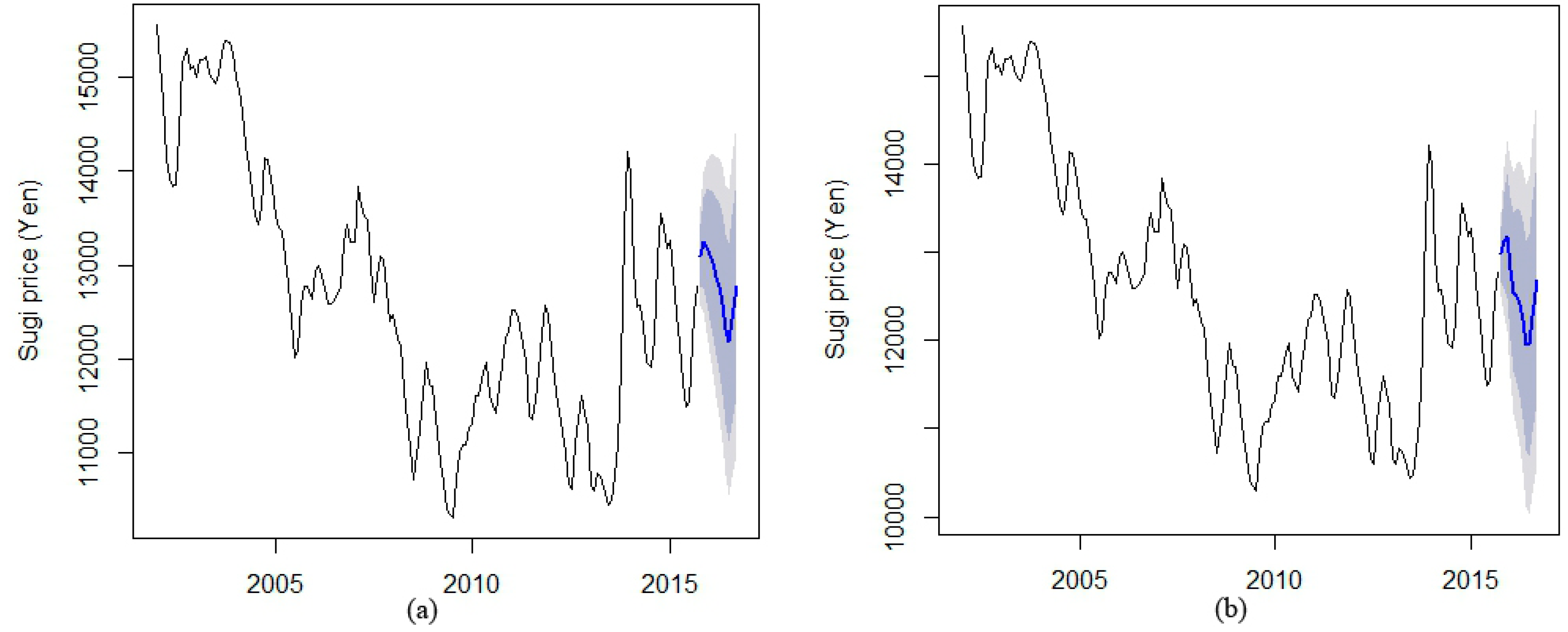
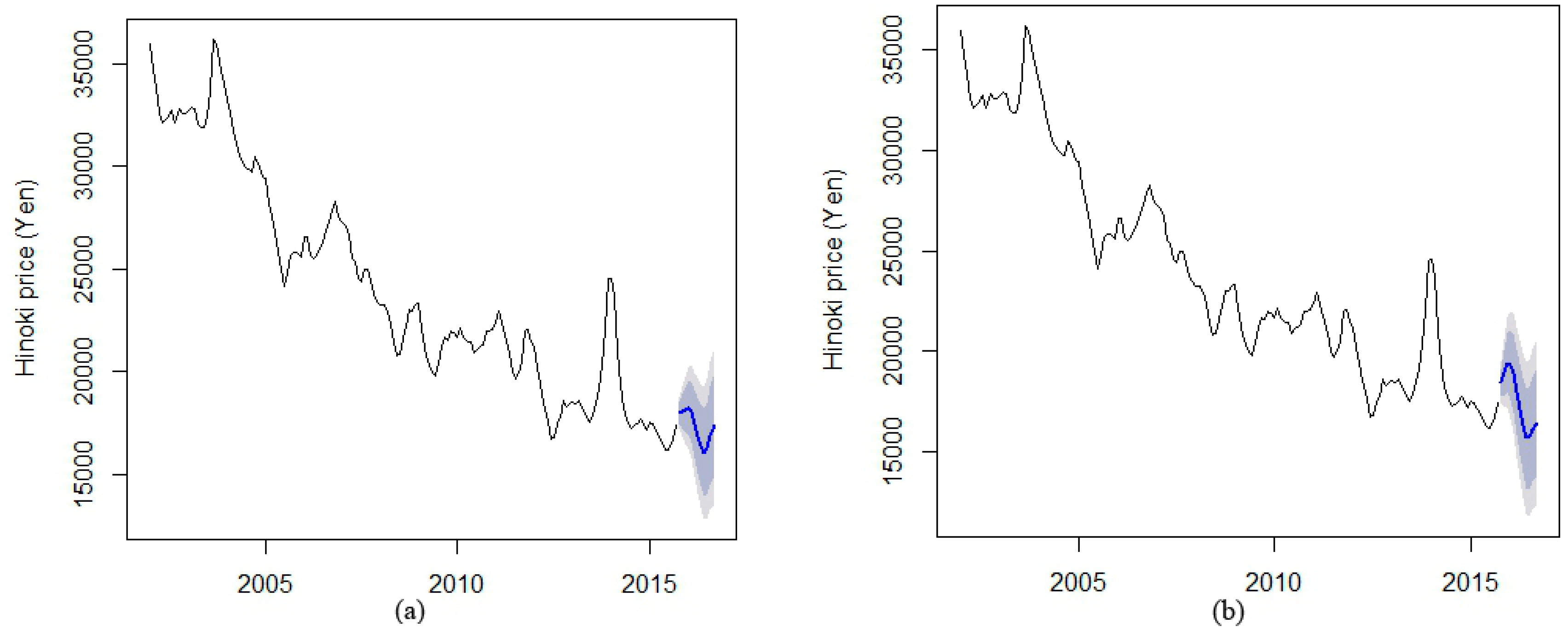
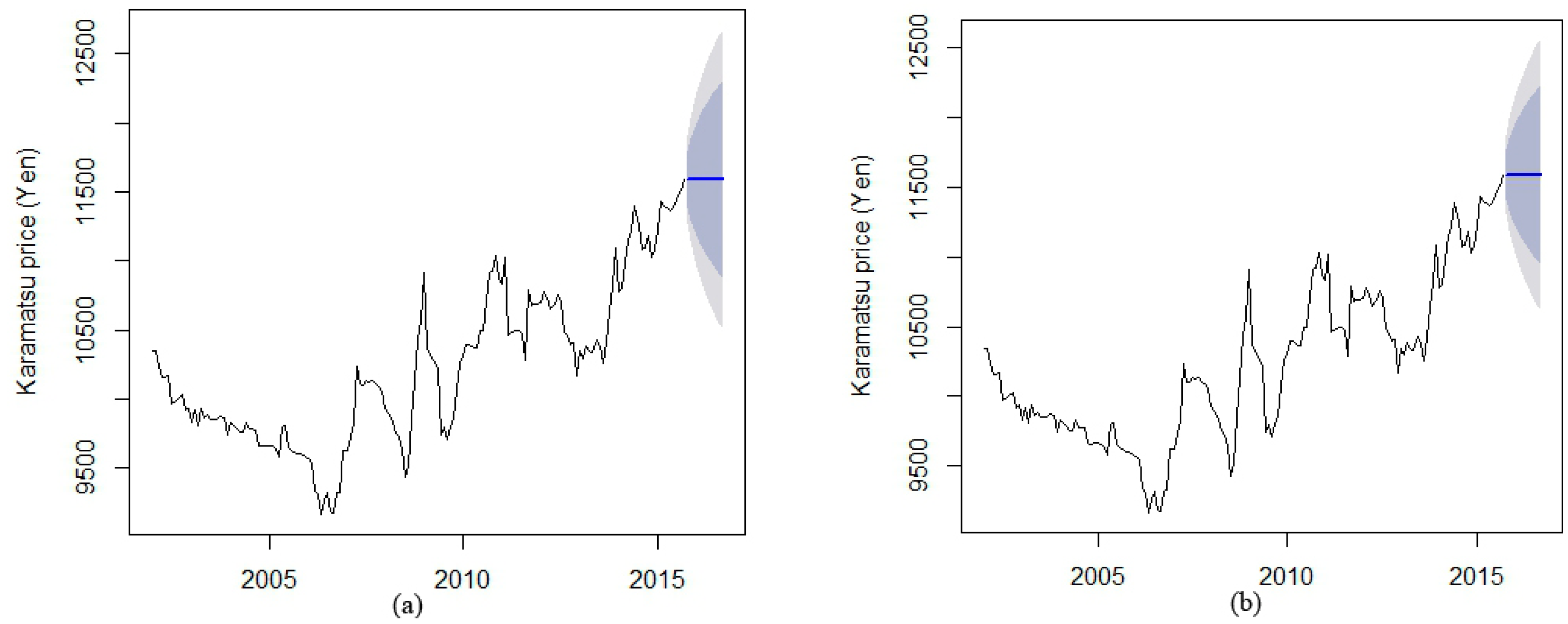
3.3. ETS Forecast Results

In using ets function in the package forecast under the R software environment, the results were shown in the form of (E, T, S), representing the error, trend and season components, respectively. The results for sugi, hinoki and karamatsu log prices are, respectively, (M, N, A), (M, Ad, A) and (M, N, N). All of these time series have multiplicative errors. Hinoki log price shows a damped trend, whereas sugi and karamatsu display no trend. As for the seasonality, the results show that sugi and hinoki experience additive seasonal movements in prices, but seasonal changes cannot be found in the karamatsu log price, which supports the aforementioned argument regarding seasonal characteristics. The smoothing parameters for sugi are α = 0.9999 and γ = 0.0001; for hinoki, they are α = 0.9999, β = 0.1412, γ = 0.0001, and ∅ = 0.8007; and for karamatsu, α = 0.9999. A high α value shows that time series values are highly affected by the previous value. A small γ value shows that the seasonal component does not change much over the years. Given that the expectation of error is zero, both the additive and multiplicative error methods gave the same forecasts but different forecast intervals.

The above estimated parameters can be substituted into the corresponding formulae in the component form [32] to obtain the final models; for sugi, its result for ETS (M, N, A) is as follows:

$$y_t=(l_{t-1}+s_{t-m})(1+{\epsilon }_t), l_t=l_{t-1}+ \alpha (l_{t-1}+s_{t-m}){\epsilon }_t, s_t=s_{t-m}+ \gamma (l_{t-1}+s_{t-m}){\epsilon }_t$$

(4)

For hinoki, ETS (M, Ad, A) is as follows:

$$y_t=(l_{t-1}+\varnothing b_{t-1}+s_{t-m})(1+{\epsilon }_t), l_t=l_{t-1}+\varnothing b_{t-1}+ \alpha (l_{t-1}+\varnothing b_{t-1}+s_{t-m}){\epsilon }_t, b_t=\varnothing b_{t-1}+ \beta (l_{t-1}+\varnothing b_{t-1}+s_{t-m}){\epsilon }_t, s_t=s_{t-m}+ \gamma (l_{t-1}+\varnothing b_{t-1}+s_{t-m}){\epsilon }_t$$

(5)

For karamatsu, ETS (M, N, N) is as follows:

$$y_t=l_{t-1}(1+{\epsilon }_t) l_t=l_{t-1}(1+\alpha {\epsilon }_t)$$

(6)

In the formulae, l_t stands for the level or smoothed value of the time series at time t, b for slope, s for seasonal component, m for number of periods in a year (here, m = 12), α, β, γ and ∅ for smoothing parameters, s_t−m for the seasonal component for the same month of the previous year. Figure 5a, Figure 6a and Figure 7a show the results by ETS for sugi, hinoki and karamatsu, respectively, while Figure 5b, Figure 6b and Figure 7b show the results by ARIMA. The right parts in both sets of figures show the results for the forecasts and the forecast intervals at probability levels of 95% (wider and brighter shadow area) and 80% (narrower and darker shadow area), respectively, for the 12 months ahead (see

Table 1. Point forecasts and forecast intervals at 80% and 95% level. Unit: Yen. ETS, exponential smoothing method; ARIMA, autoregressive integrated moving average.

Log	Month	ETS					ARIMA
		Point Forecasts	Low 80%	High 80%	Low 95%	High 95%	Point Forecasts	Low 80%	High 80%	Low 95%	High 95%
Sugi	15 October	13,045	12,704	13,386	12,523	13,567	12,913	12,604	13,223	12,440	13,387
	15 November	13,189	12,704	13,674	12,447	13,931	13,072	12,525	13,620	12,235	13,910
	15 December	13,151	12,556	13,746	12,241	14,061	13,129	12,427	13,832	12,055	14,204
	16 January	13,058	12,372	13,744	12,009	14,107	12,753	11,944	13,562	11,516	13,990
	16 February	12,972	12,207	13,738	11,802	14,143	12,489	11,593	13,384	11,119	13,858
	16 March	12,827	11,991	13,663	11,549	14,106	12,442	11,466	13,418	10,949	13,935
	16 April	12,716	11,816	13,615	11,340	14,092	12,367	11,315	13,419	10,759	13,976
	16 May	12,534	11,576	13,492	11,069	13,999	12,175	11,051	13,298	10,456	13,893
	16 June	12,260	11,249	13,270	10,715	13,804	11,888	10,697	13,079	10,067	13,709
	16 July	12,122	11,063	13,181	10,502	13,741	11,888	10,634	13,142	9970	13,806
	16 August	12,368	11,261	13,476	10,675	14,062	12,213	10,899	13,527	10,203	14,222
	16 September	12,720	11,563	13,877	10,951	14,489	12,628	11,256	13,999	10,530	14,725
Hinoki	15 October	17,909	17,409	18,408	17,145	18,672	18,366	17,711	19,022	17,364	19,368
	15 November	17,989	17,207	18,772	16,792	19,187	18,804	17,691	19,917	17,102	20,507
	15 December	18,039	17,027	19,051	16,492	19,587	19,322	17,853	20,791	17,076	21,568
	16 January	18,113	16,897	19,328	16,254	19,971	19,256	17,514	20,998	16,591	21,920
	16 February	17,952	16,553	19,351	15,812	20,092	18,848	16,894	20,803	15,859	21,838
	16 March	17,346	15,781	18,910	14,953	19,739	17,886	15,763	20,009	14,639	21,132
	16 April	16,801	15,088	18,515	14,180	19,423	17,046	14,787	19,305	13,591	20,501
	16 May	16,336	14,486	18,186	13,507	19,166	16,261	13,889	18,633	12,633	19,889
	16 June	15,966	13,990	17,942	12,944	18,988	15,614	13,146	18,081	11,839	19,388
	16 July	16,131	14,036	18,226	12,927	19,335	15,606	13,055	18,157	11,705	19,508
	16 August	16,758	14,545	18,971	13,374	20,142	16,041	13,416	18,665	12,027	20,054
	16 September	17,320	14,991	19,650	13,757	20,883	16,389	13,699	19,079	12,275	20,503
Karamatsu	15 October	11,546	11,342	11,750	11,234	11,858	11,546	11,363	11,729	11,266	11,826
	15 November	11,546	11,257	11,835	11,105	11,987	11,546	11,287	11,805	11,150	11,942
	15 December	11,546	11,193	11,899	11,005	12,087	11,546	11,229	11,863	11,061	12,031
	16 January	11,546	11,138	11,954	10,922	12,170	11,546	11,180	11,912	10,986	12,106
	16 February	11,546	11,090	12,002	10,848	12,244	11,546	11,136	11,956	10,920	12,172
	16 March	11,546	11,046	12,046	10,781	12,311	11,546	11,097	11,995	10,860	12,232
	16 April	11,546	11,006	12,086	10,720	12,372	11,546	11,061	12,031	10,805	12,287
	16 May	11,546	10,969	12,123	10,663	12,429	11,546	11,028	12,064	10,754	12,338
	16 June	11,546	10,934	12,158	10,609	12,483	11,546	10,996	12,096	10,706	12,386
	16 July	11,546	10,900	12,192	10,559	12,533	11,546	10,967	12,125	10,660	12,432
	16 August	11,546	10,869	12,223	10,511	12,581	11,546	10,938	12,154	10,617	12,475
	16 September	11,546	10,839	12,253	10,464	12,628	11,546	10,911	12,181	10,576	12,516

for 12-months-ahead forecast and forecast interval values).

3.4. ARIMA Forecast Results

These three time series are not stationary, as shown by their actual values in their left parts in either both sets of figures; their levels changed and did not converge to some constant value. The Augmented Dickey-Fuller (ADF) test, a unit root test, was implemented [36,37]. Package tseries in R was used in which the null hypothesis is that the time series has a unit root and is not stationary, and an alternative hypothesis we adopted in this case study is that it is “stationary”. For sugi, Dickey-Fuller = −1.860 (p-value = 0.635); after differencing, Dickey-Fuller = −7.142 (p-value < 0.01). For hinoki, Dickey-Fuller = −2.655 (p-value = 0.303); after differencing, Dickey-Fuller =−6.918 (p-value < 0.01). For karamatsu, Dickey-Fuller = −3.252 (p-value = 0.082); after differencing, Dickey-Fuller = −6.307 (p-value < 0.01). p-values above 0.05 in the ADF tests for the original time series show that the null hypothesis that original time series is not stationary and cannot be rejected by a 5% significant level, i.e., providing no evidence against the need for differencing, but that after differencing, p-values become less than 0.01, showing that further integration of a 2nd order can be rejected, and the 1st differences become stationary at a 1% significance level. That is, a degree of one is suitable for the integrated part of the ARIMA models.

By implementing the Arima function in the package forecast, we obtained the following result for sugi as the best model due to its lowest AICc: ARIMA (2, 1, 0) (2, 1, 1), representing two non-seasonal autoregressive terms, two seasonal autoregressive terms, and one seasonal moving averages term. Their coefficients and standard errors are, respectively, 0.457 (0.079), −0.245 (0.085), −0.595 (0.145), −0.441 (0.118), and −0.367 (0.165). All of them are significant at a 1% significance level, though in forecasting, it is not important to pursue significance parameters. When summarizing this result, the following model can be obtained.

Y_t = 1.457Y_t−1 − 0.702Y_t−2 + 0.245Y_t−3 + 0.405Y_t−12 − 0.590Y_t−13 + 0.284Y_t−14 − 0.099Y_t−15 + 0.154Y_t−24 − 0.224Y_t−25 + 0.108Y_t−26 − 0.038Y_t−27 + 0.441Y_t−36 − 0.643Y_t−37 + 0.310Y_t−38 − 0.108Y_t−39 + e_t − 0.367e_t−12

(7)

By fitting it into the ARIMA model, we obtained the best hinoki log price model as ARIMA (2, 1, 1) (0, 1, 2), with two non-seasonal autoregressive terms, one non-seasonal moving average term, and two seasonal moving average terms. Their coefficients and standard errors are: 1.306 (0.087), −0.398 (0.076), −0.932 (0.057), −1.104 (0.092), and 0.352 (0.109). All of these parameters are also significant at a 1% significance level. The model is as follows:

Y_t = 2.306Y_t−1 − 1.704Y_t−2 + 0.398Y_t−3 + Y_t−12 − 2.306Y_t−13 + 1.704Y_t−14 − 0.398Y_t−15+ e_t − 0.932e_t−1 − 1.104e_t−12 + 1.029e_t−13 + 0.352e_t−24 – 0.328e_t−25

(8)

The best karamatsu log price model has the form as ARIMA (0, 1, 0), with no seasonal terms, autoregressive terms, or moving average terms. This type of time series is usually called a random walk [35]. The model can be written as:

Y_t = Y_t−1 + e_t

(9)

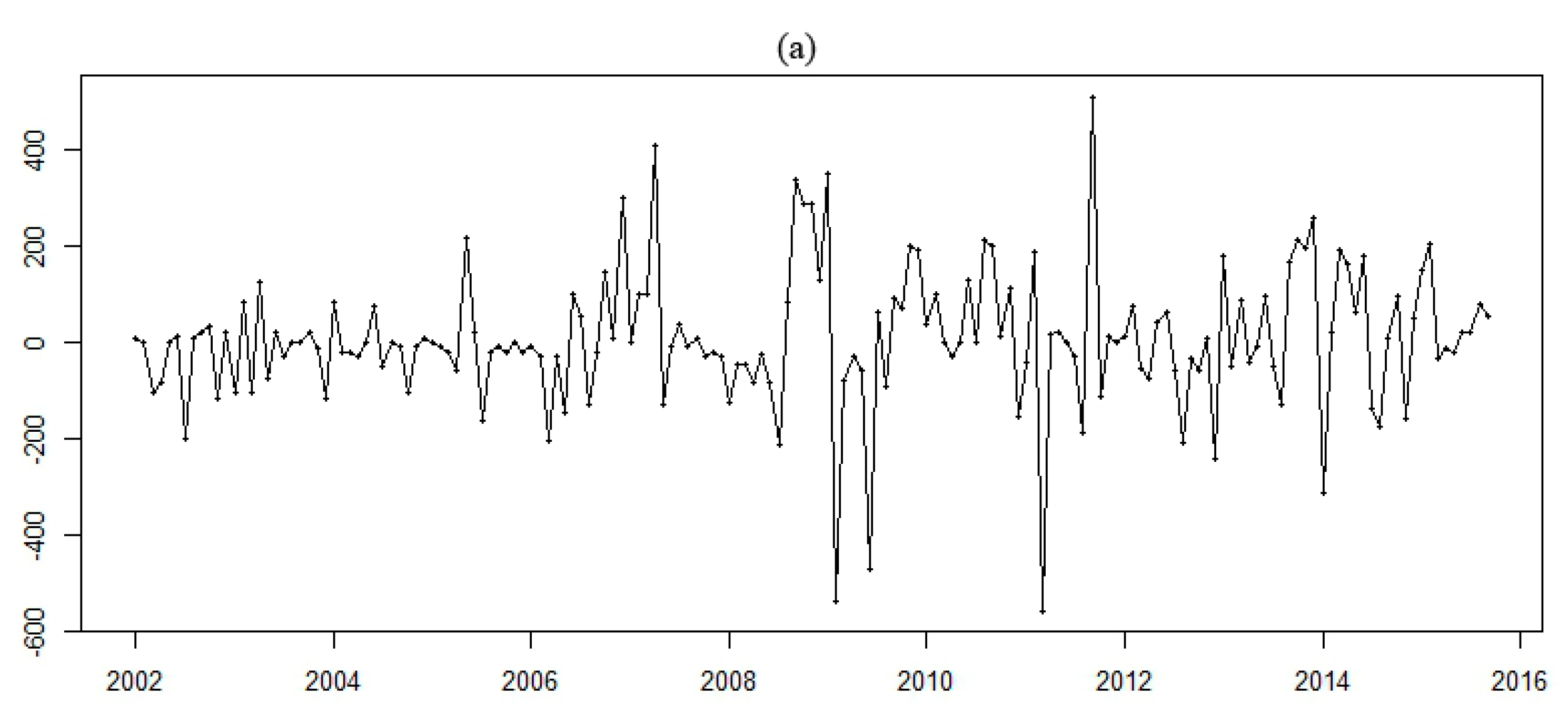
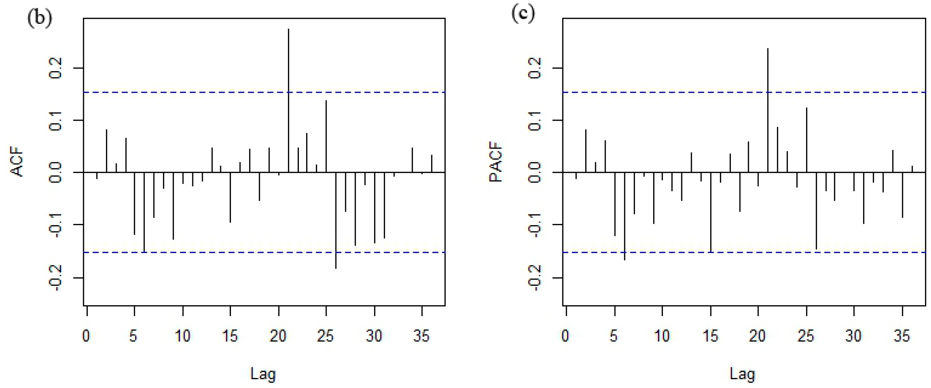
3.5. Diagnostic Check of Residuals in ARIMA Models

Finally, we need to verify the adequacy of our ARIMA models by checking their residuals. By fitting a model, we can obtain fitted values and residuals. For a forecasting model, we have observed values and forecasts based on previous observed values, and the differences are residuals: $e_t=y_t-{\widehat{y}}_t.$ Residuals should have two properties: uncorrelated and zero mean [32]. Correlations between residuals mean that the model is not fitted well because patterns remained in the residuals and should be included in the model. In addition, if the mean of residuals is not zero, then the forecasts are biased. It would be better also to check two other properties for ideal residuals: constant variance and normal distribution [32].

For the three ARIMA models, we first checked residuals’ correlations. Figure 8 shows residuals and their autocorrelations and partial autocorrelations with lags of up to 36 for the sugi log price. No pattern can be found in Figure 8a, though some irregular residuals existed. Figure 8b,c show that no significant correlations were confirmed. The situations for hinoki were similar. Figure 9 showed the analysis of the prices for karamatsu logs. Similarly, some irregular residuals were found in Figure 9a, but no pattern was confirmed. Two significant autocorrelations and partial correlations, respectively, were found by checking Figure 9b,c but most of them with a lag over 20. This result can be ignored by considering it an accidental result. We then implemented an ADF test, and the Dickey-Fuller results were −5.992, −5.360, and −6.283, respectively, for sugi, hinoki, and karamatsu. For all of the cases, p-value <0.01, which shows that they are stationary. Finally, we implemented the Box-Ljung test [38]. The results for sugi, hinoki, and karamatsu are χ² = 22.660 (p-value = 0.540), 15.874 (p-value = 0.893), and 32.014 (p-value = 0.127), which means that these residuals were not distinguishable from a white noise series.

3.6. Measuring the Accuracy of Forecasts

To measure the forecast accuracy, we divided our data set into two parts: sample data and out-of-sample data. We dealt with two forecast periods here: 12 months and 6 months. We established the objective of the research as being to forecast monthly prices and acknowledged the forecasting as being short-term; therefore, being able to forecast one year ahead or some months (less than 12 months) ahead accurately is important. The errors for forecasting sugi, hinoki, and karamatsu log prices for 12 months ahead by ETS and ARIMA were shown in

Table 2. Forecast errors for 12-months-ahead forecasts. “Kara.” stands for karamatsu. The smallest error among the three methods is shown in bold letters. Snaïve method is applied to sugi and hinoki, while the naïve method to karamatsu. MAPE, mean absolute percentage error; MAE, mean absolute error; RMSE, root mean square error.

Valuations		MAPE (%)			MAE (Yen)			RMSE (Yen)
		Snaïve/Naïve	ETS	ARIMA	Snaïve/Naïve	ETS	ARIMA	Snaïve/Naïve	ETS	ARIMA
1	Sugi	3.96	4.77	5.57	504	578	685	670	697	748
	Hinoki	19.01	3.25	1.64	3273	545	282	4065	626	332
	Kara.	2.20	2.20	2.20	252	252	252	285	285	285
2	Sugi	4.99	3.33	2.37	639	416	300	872	457	347
	Hinoki	19.74	2.44	1.74	3401	418	301	4094	479	378
	Kara.	1.93	1.93	1.93	220	220	220	261	261	261
3	Sugi	5.82	3.24	2.26	740	407	289	967	455	360
	Hinoki	19.90	3.29	2.52	3432	571	436	4101	708	516
	Kara.	1.26	1.26	1.26	142	142	142	151	151	151
4	Sugi	6.53	3.33	2.05	825	426	263	1045	498	342
	Hinoki	19.60	5.45	8.84	3386	940	1523	4091	1035	1577
	Kara.	1.42	1.42	1.42	158	158	158	208	208	208
5	Sugi	7.25	2.75	2.38	913	354	309	1126	429	395
	Hinoki	18.92	14.06	6.07	3278	2429	1051	4069	2607	1139
	Kara.	1.17	1.17	1.17	132	132	132	147	147	147
6	Sugi	7.98	2.32	1.74	1007	301	225	1218	373	284
	Hinoki	18.23	15.43	7.50	3166	2678	1304	4043	2977	1442
	Kara.	1.19	1.19	1.19	135	135	135	160	160	160
7	Sugi	8.92	2.64	1.60	1125	346	211	1323	445	319
	Hinoki	17.46	15.54	8.20	3046	2720	1432	3990	2854	1592
	Kara.	1.95	1.96	1.95	220	221	220	257	258	257
8	Sugi	10.04	3.17	3.43	1266	400	444	1418	456	512
	Hinoki	16.51	34.81	22.13	2922	6161	3926	3890	6397	4029
	Kara.	3.39	3.39	3.39	380	380	380	402	402	402
9	Sugi	11.51	12.42	5.86	1457	1571	738	1571	1588	782
	Hinoki	15.37	40.29	24.09	2841	7177	4305	3767	7642	4520
	Kara.	3.11	3.10	3.11	348	346	348	377	375	377
10	Sugi	13.05	16.79	12.67	1675	2125	1602	1830	2204	1653
	Hinoki	14.08	65.79	30.81	2759	11,862	5573	3622	12,709	5931
	Kara.	1.16	1.16	1.16	129	129	129	170	170	170

. As for other lengths, from one to five months, from seven to 11 months, the results for sugi and hinoki were shown in supplementary materials (Tables S1–S10).

Table 2 shows 10 valuations of forecast errors of 12-months-ahead forecasts. Firstly, data from October 2014 to September 2015 were taken as out-of-sample data, while the data from January 2002 to September 2014 were taken as sample data. In the next nine valuations, by keeping 12 months as the forecast period and deleting the last datum in the series every time and moving backward, we obtained nine sets of sample data and out-of-sample data. Thus, the second sample data were from January 2002 to August 2014, and out-of-sample data were from September 2014 to August 2015. Snaïve was used for sugi and hinoki accuracy valuations, but a naïve method was used for karamatsu because the karamatsu log price did not show obvious seasonality.

As shown in Table 2, MAPE, MAE, and RMSE have similar results in comparing the accuracy of forecasts among ETS, ARIMA, and Snaïve method to sugi and hinoki or naïve method to karamatsu; i.e., when MAPE value is the smallest for a method among the three methods, MAE and RMSE values are also smallest for this method. Valuation 1 was the case in which the most recent sample data and out-of-sample data were used. For the sugi log price, ETS had a smaller error than ARIMA, but both ETS and ARIMA had larger errors than the Snaïve method. The results showed the error ranged from 3.96% to 5.57% by MAPE, from 504 Yen to 685 Yen by MAE, and from 670 Yen to 748 Yen by RMSE. For the hinoki log price in Valuation 1, its forecast accuracy was much better. The smallest forecast errors were from ARIMA, which were 1.64% by MAPE, 282 Yen by MAE, and 332 Yen by RMSE. The ETS results were not as good as those of ARIMA but were better than those of the Snaïve method. As for the karamatsu log price in Valuation 1, ETS and ARIMA resulted in the same errors as the naïve method.

By comparing the errors for sugi and hinoki over 10 valuations, Valuations 9 and 10 gave the largest errors due to the impact of the irregular level of prices at the end of 2013. Among the 10 valuations, it can be found that for sugi, ETS had smaller errors twice (i.e., for Valuations 1 and 8); for hinoki, ETS had a better error only once (i.e., for Valuation 4); and in all other cases ARIMA showed smaller errors for sugi and hinoki. As for karamatsu, ETS and ARIMA had the same errors as those by naïve method, except in the two valuations due to the rounding errors (i.e., Valuations 7 and 9).

MAPE, MAE, and RMSE are metrics that are used to summarize the errors for the whole forecast periods. When changing the length of forecast periods, the results expressed by these metrics might also change. Forecasters occasionally need to know the forecast for the next 6 months rather than the next 12 ones. Hence, we also measured the accuracy of forecasts in 6-months-ahead forecasts 10 times. Similarly, we kept the length of 6 months for out-of-sample data and, for each time, deleted the last datum and moved the dataset backward to obtain a new dataset. Similarly to the results in Table 2, in the majority of cases of 6-months-ahead forecasts for sugi and hinoki log prices, ARIMA had smaller errors than ETS and, as for the karamatsu log prices, ETS and ARIMA had the same errors as those obtained when using the naïve method (

Table 3. Forecast errors for 6-months-ahead forecasts. “Kara.” stands for karamatsu. The smallest error among the three methods are shown in bold letters. Snaïve method is applied to sugi and hinoki, while naïve method to karamatsu.

Valuations		MAPE (%)			MAE (Yen)			RMSE (Yen)
		Snaïve/Naïve	ETS	ARIMA	Snaïve/Naïve	ETS	ARIMA	Snaïve/Naïve	ETS	ARIMA
1	Sugi	3.47	2.87	2.25	414	345	273	427	362	299
	Hinoki	7.63	2.34	2.99	1264	388	496	1460	409	521
	Kara.	0.44	0.44	0.44	50	50	50	71	71	71
2	Sugi	3.13	4.09	2.63	370	483	312	404	519	330
	Hinoki	11.29	4.54	1.46	1889	751	240	2162	776	284
	Kara.	0.39	0.39	0.39	44	44	44	44	46	46
3	Sugi	2.85	6.33	6.70	336	752	798	391	791	821
	Hinoki	16.58	5.92	1.12	2817	980	187	3345	1057	221
	Kara.	1.49	1.49	1.49	170	170	170	171	171	171
4	Sugi	3.17	4.12	2.83	388	493	344	460	567	372
	Hinoki	22.13	7.12	2.09	3806	1194	350	4387	1294	404
	Kara.	2.54	2.54	2.54	290	290	290	297	297	297
5	Sugi	3.78	3.99	2.16	480	487	268	590	599	311
	Hinoki	27.70	4.72	1.91	4779	798	325	5274	958	356
	Kara.	2.55	2.55	2.55	290	290	290	315	315	315
6	Sugi	2.98	5.06	3.70	387	641	472	538	705	513
	Hinoki	30.42	2.54	2.08	5268	434	359	5553	563	395
	Kara.	1.44	1.44	1.44	163	163	163	177	177	177
7	Sugi	4.45	2.59	4.08	594	333	531	847	398	579
	Hinoki	30.38	1.59	2.25	5282	275	392	5560	332	422
	Kara.	1.42	1.42	1.42	161	161	161	203	203	203
8	Sugi	6.84	2.86	2.58	907	381	342	1166	434	402
	Hinoki	28.19	3.27	2.41	4914	570	421	5371	610	478
	Kara.	0.99	0.99	0.99	112	112	112	164	164	164
9	Sugi	8.78	3.28	2.82	1143	436	374	1310	491	455
	Hinoki	23.22	4.97	3.23	4046	867	564	4737	928	634
	Kara.	1.28	1.28	1.28	142	142	142	158	158	158
10	Sugi	9.88	3.81	2.06	1262	502	274	1405	577	393
	Hinoki	17.07	4.54	9.18	2967	793	1602	3772	909	1680
	Kara.	2.47	2.47	2.47	274	274	274	285	285	285

). Similarly, the errors from the earliest sample data for hinoki by ARIMA, as shown in Valuation 10, were also high compared with other valuations for hinoki by ARIMA: 9.18% by MAPE, 1602 Yen by MAE, and 1680 Yen by RMSE.

ETS and ARIMA occasionally give rather different forecast results as shown in Table 1. It is difficult to say which method is definitively better than the other, even though ARIMA makes forecasts with smaller errors in most cases in this research. Therefore, in order to find a method by which we can forecast prices with smaller errors, we attempted another method in which we combined the forecasts from ETS and ARIMA to obtain average point forecasts for sugi and hinoki. Karamatsu is not dealt with because it is a random walk, and ETS and ARIMA gave the same point forecasts with the naïve method. The forecast errors by using this combined method are shown in

Table 4. Forecast errors using average method for 12- and 6-months ahead forecasts.

Valuations		12-Months-Ahead			6-Months-Ahead
		MAPE	MAE	RMSE	MAPE	MAE	RMSE
1	Sugi	5.09	620	714	2.56	309	329
	Hinoki	2.18	369	414	2.66	442	456
2	Sugi	2.85	357	394	3.36	398	421
	Hinoki	1.96	337	409	2.85	469	509
3	Sugi	2.72	344	398	6.52	775	805
	Hinoki	2.91	503	604	2.88	475	552
4	Sugi	2.66	342	415	3.32	399	461
	Hinoki	1.70	293	323	4.61	772	836
5	Sugi	2.42	314	400	2.76	337	422
	Hinoki	4.16	718	768	3.23	548	640
6	Sugi	1.99	258	320	4.38	556	605
	Hinoki	4.02	698	797	2.02	346	431
7	Sugi	2.07	273	374	3.17	410	471
	Hinoki	11.87	2076	2216	1.57	274	337
8	Sugi	1.26	163	213	2.71	360	413
	Hinoki	28.47	5043	5211	2.84	496	537
9	Sugi	9.14	1155	1176	3.05	405	471
	Hinoki	32.19	5741	6077	4.10	715	775
10	Sugi	14.73	1863	1922	2.91	385	477
	Hinoki	48.30	8717	9317	2.34	408	410

. For 12-months-ahead forecasts, in Valuations 4, 5, and 6 for hinoki log prices and Valuation 8 for sugi log prices, the errors by the combined method were the smallest among Snaïve, ETS, ARIMA, which are shown in Table 2, and this combined method is based on all three error metrics. For 6-months-ahead forecasting, in Valuations 10 for the hinoki log price, the results from the combined method were the best based on all three error metrics. For most cases, errors from the combined method were found to fall between those observed for ETS and ARIMA models. In other words, the forecasts using the combined method were not the worst forecasts and were occasionally better than both the ETS and ARIMA forecasts.

4. Discussion

As the saying goes, all forecasts are wrong, but some might be useful. In this research, we used the national average log price data of sugi, hinoki, and karamatsu; ETS and ARIMA methods; and the package forecast in software R [16]. We checked the seasonality, the trend, and obtained 12-months-ahead forecasts for sugi, hinoki, and karamatsu. The fact that Japanese sugi and hinoki log prices are seasonal but karamatsu prices are not is well reflected in the ETS and ARIMA models. In most cases, ARIMA gave better results than ETS for sugi and hinoki. These findings are useful for the short-term forecasting of Japanese domestic log prices. Actually, though ETS and ARIMA adopt different modeling and estimation strategies and algorithms, additive error ETS models are all special cases of ARIMA models, while the non-linear ETS models cannot find equivalents in ARIMA [32]. Our ETS models all have multiplicative errors; therefore, the best models by ETS and ARIMA in this case do not have equivalents to each other. For karamatsu log prices, the forecasts by ETS and ARIMA are the same as the ones by the naïve method, but their forecasting intervals are different.

Because forecasting deals with stochastic issues, no one can be sure about their forecasts. Showing forecasting intervals is a good way to reflect the extent of possible variations. If actual prices are approaching the upper or lower limits, this should raise a high alert in terms of risk management. Providing such data would be useful to avoid the mismatch between supply and demand and, thus, the sharp fall or rise of log prices.

This research used univariate time series analysis for forecasting. Sometimes, structural time series models are useful for forecasting, as they incorporate terms of interest into the model, though one has to forecast or assume those terms first. In the case of forecasting price, however, it becomes complicated. According to economics theory, the price of a commodity is an endogenous variable that is determined by the relationship between supply and demand in the market. Price shifts with the changes in income, consumers’ preferences, cost of production elements, technological changes, prices of other related commodities, among other factors. Prices can be forecasted by taking these factors into account. For example, Organization of the Petroleum Exporting Countries (OPEC) quota, OPEC production, and industrial stock level of oil can be used to forecast short-term oil price [39]. However, there are not many empirical studies on price forecasting by using structural time series models, perhaps due to the difficulties in quantifying the related factors and those factors must be forecasted prior to forecasting prices. With univariate forecasting approaches, the only variable is log price in this research, which makes forecasting simple and sometimes useful. Of course, the ETS method simply decomposes a time series into trend, seasonal, and error components without taking other elements into account, such as cyclical movements. As for ARIMA models, it might be a good idea to add exogenous variables to the model [40,41]. Furthermore, it is also worthwhile to apply equilibrium, structural, and reduced form models in forecasting the prices of Japanese logs.

Abenomics, a policy that went into effect in Japan in December 2012, ensured that corrections to the excessive yen appreciation were made. In addition, when the plan to raise consumption tax from 5% to 8% in April 2014 was communicated to the public in October 2013, a spike in demand for wood house construction led to sharp increases in sugi and hinoki log prices from October 2013 to January 2014. After this period, hinoki log prices dropped to their earlier level, whereas sugi log prices dropped and fluctuated at a higher level than previously. These contextual changes made short-term forecasts from this specific period uncertain. Fortunately, concerns that increased tax would case an economic recession have not become a reality. These price fluctuations in sugi and hinoki can be taken as irregular movements. That is, the structural changes in the logs market in Japan have not occurred.

However, any factors that affect demand and supply, including any changes in the international and domestic economic environment, might affect prices. The impact of the increase in consumption tax (from 8% to 10%) in the near future and fluctuations in exchange rates were not discussed in the research. Another important issue is the impact of the general price level. Constant price data were used in the research. Given the low inflation value, it did not make a difference in comparison to using current value log prices. Using a constant value mitigated the impact of general price changes. However, it will be necessary to recalculate the forecasts during periods of higher inflation. In addition, impacts of changes in the international market and policy are also not dealt with in the research. Incorporating influencing factors into forecasts of log prices should also be a focus of further research.

References

1. Endo, K. Why Log Prices Collapsed: Reasons, Mechanism and Measures; National Forestry Extension Association: Tokyo, Japan, 2013; p. 144. [Google Scholar]
2. Mochizuki, R. A statistical study on fluctuations in prices of main forest products. Bull. Tokyo Imp. Univ. For. 1929, 7, 1–121. [Google Scholar]
3. Mitsui, T. On seasonal movements of timber prices. In Forestry Economic and Policy Materials; The Japan Forestry Association: Tokyo, Japan, 1938; Volume 3, pp. 43–56. [Google Scholar]
4. Shindo, R. The Future of the Wood Market and Industry; Price Agency: Tokyo, Japan, 1949; p. 221. [Google Scholar]
5. Akai, H. Research on Trend of Timber Prices; Bulletin of Forestry Management Institute: Tokyo, Japan, 1965; Volume 63, p. 302. [Google Scholar]
6. Matsumoto, K. Research on Cyclic Fluctuations of Timber Prices; Bulletin of Forestry Management Institute: Tokyo, Japan, 1966; Volume 63, p. 92. [Google Scholar]
7. Mori, Y. A Study on the Time-Series-Analysis of Lumber Price in Japan. J. Jpn. For. Soc. 1970, 52, 227–237. [Google Scholar]
8. Matsushita, K. Applications of spectral analysis to the cyclical fluctuations of lumber prices. Trans. Jpn. For. Soc. 1984, 95, 17–18. [Google Scholar]
9. Matsushita, K.; Handa, R. The cyclical fluctuation of lumber price. Bull. Kyoto Univ. For. 1981, 53, 76–86. [Google Scholar]
10. Yukutake, K. Time series analysis of timber price fluctuation after World War II. The Current State of Japanese Forestry. In Proceedings of the IUFRO World Congress, Kyoto, Japan, 6–17 September 1981; Volume 1, pp. 41–54.
11. Yukutake, K.; Yoshimoto, A.; Higuchi, Y. Time series analysis of timber prices at two private auction markets in Kyushu Japan. Jpn. J. For. Plan. 2004, 38, 61–74. [Google Scholar]
12. Kuboyama, H.; Tachibana, S. Statistical analysis on price trend of softwood roundwood. Kanto J. For. Res. 2014, 65, 9–12. [Google Scholar]
13. Elias, R.J.; Montgomery, D.C.; Kulahci, M. An overview of short-term statistical forecasting methods. Int. J. Manag. Sci. Eng. Manag. 2006, 1, 17–36. [Google Scholar]
14. Makridakis, P.; Wheelwright, S.C.; Hyndman, R.J. Foresting: Methods and Applications, 3rd ed.; Wiley: New York, NY, USA, 1998; p. 656. [Google Scholar]
15. Hyndman, R.J.; Koehler, A.B.; Ord, J.K.; Synder, R.D. Forecasting with Exponential Smoothing: The State Space Approach; Springer: Berlin, Germany, 2008; p. 359. [Google Scholar]
16. R Core Team. R: A Language and Environment for Statistical Computing. R Foundation for Statistical Computing, Vienna, Austria. Available online: http://www.R-project.org/ (accessed on 2 February 2015).
17. Hyndman, R.J. Forecasting Functions for Time Series and Linear Models. Available online: http://github.com/robjhyndman/forecast (accessed on 25 October 2015).
18. Forestry Agency. Statistical Handbook of Forest and Forestry; Forestry Agency, Ministry of Agriculture, Forestry and Fisheries: Tokyo, Japan, 2013; p. 262. [Google Scholar]
19. Forestry Agency. Balance Sheet of Wood. Available online: http://www.rinya.maff.go.jp/j/press/kikaku/pdf/150929-02.pdf (accessed on 5 December 2015).
20. MAFF. Ministry of Agriculture, Forestry and Fisheries. Available online: http://www.maff.go.jp/j/tokei/kouhyou/kensaku/bunya5.html (accessed on 15 October 2015).
21. Findley, D.F.; Monsell, B.C.; Bell, W.R.; Otto, M.C.; Chen, B.C. New Capabilities and methods of the X-12-ARIMA seasonal-adjustment Program. J. Bus. Econ. Stat. 1998, 16, 127–152. [Google Scholar] [CrossRef]
22. Makridakis, S.; Hibon, M. The M3-Competition: Results, conclusions and implications. Int. J. Forecast. 2000, 16, 451–476. [Google Scholar] [CrossRef]
23. Hyndman, R.J.; Koehler, A.B.; Snyder, R.D.; Grose, S. A state space framework for automatic forecasting using exponential smoothing methods. Int. J. Forecast. 2002, 18, 439–454. [Google Scholar] [CrossRef]
24. Sanders, D.R.; Manfredo, M.R. USDA livestock price forecasts: A comprehensive evaluation. J. Agric. Resour. Econ. 2003, 28, 316–334. [Google Scholar]
25. Sanders, D.R.; Manfredo, M.R. Rationality of U.S. Department of Agriculture Livestock price forecasts: A unified approach. J. Agric. Appl. Econ. 2007, 39, 75–85. [Google Scholar]
26. Gelper, S.; Fried, R.; Croux, C. Robust forecasting with exponential and Holt-Winters smoothing. J. Forecast. 2010, 29, 285–300. [Google Scholar] [CrossRef]
27. Hassani, H.; Silva, S.S.; Gupta, R.; Segnon, M.K. Forecasting the price of gold. Appl. Econ. 2015, 47, 4141–4152. [Google Scholar] [CrossRef]
28. Guttormsen, A.G. Forecasting weekly salmon prices: Risk management in fish farming. Aquac. Econ. Manag. 1999, 3, 159–166. [Google Scholar] [CrossRef]
29. Holt, C.C. Forecasting seasonals and trends by exponentially weighted moving averages (a reprinted version). Int. J. Forecast. 2004, 20, 5–10. [Google Scholar] [CrossRef]
30. Brown, R.G. Statistical Forecasting for Inventory Control; McGraw/Hill: New York, NY, USA, 1959; p. 223. [Google Scholar]
31. Winters, P.R. Forecasting Sales by Exponentially Weighted Moving Averages. Manag. Sci. 1960, 6, 324–342. [Google Scholar] [CrossRef]
32. Hyndman, R.J.; Athanasopoulos, G. Forecasting: Principles and Practice. Available online: http://otexts.org/fpp/ (accessed on 10 September 2015).
33. Burnham, K.P.; Anderson, D.R. Model Selection and Multimodel Inference: A Practical Information-Theoretic Approach, 2nd ed.; Springer-Verlag: Berlin, Germany, 2002; p. 488. [Google Scholar]
34. Hamilton, J.D. Time Series Analysis; Princeton University Press: Princeton, NJ, USA, 1994; p. 799. [Google Scholar]
35. Harvey, A.C. Forecasting, Structural Time Series and the Kalman Filter; Cambridge University Press: Cambridge, UK, 1989; p. 554. [Google Scholar]
36. Said, S.E.; Dickey, D.A. Testing for unit roots in autoregressive-Moving Average Models of Unknown Order. Biometrika 1984, 71, 599–607. [Google Scholar] [CrossRef]
37. Trapletti, A.; Hornik, K.; LeBaron, B. Time Series Analysis and Computational Finance. Package “tseries” in R. Available online: https://cran.r-project.org/web/packages/tseries/tseries.pdf (accessed on 10 December 2015).
38. Ljung, G.; Box, G. On a measure of lack of fit in Time Series Models. Biometrika 1978, 65, 297–303. [Google Scholar] [CrossRef]
39. Zamani, M. An econometrics forecasting model of short term oil spot price. In Proceedings of the 6th IAEE European Conference, Zurich, Switzerland, 2–3 September 2004.
40. Nogales, F.J.; Contreras, J.; Conejo, A.J.; Espinola, R. Forecasting next-day electricity prices by time series models. IEEE Trans. Power Syst. 2002, 17, 342–348. [Google Scholar] [CrossRef]
41. Weron, R. Electricity price forecasting: A review of the state-of-the-art with a look into the future. Int. J. Forecast. 2014, 30, 1030–1081. [Google Scholar] [CrossRef]
Figure 1. Top production regions of sugi, hinoki, and karamatsu logs. The darkest color shows the production regions for karamatsu; the brightest color for production regions of sugi; while others for hinoki.
Forests 07 00094 g001
Figure 2. Annual and monthly sugi log prices: (a) Annual changes of sugi log prices against months; (b) monthly subseries of sugi log prices. In Figure 2b, the horizontal bars show the mean prices for the monthly subseries, and polygonal lines show the changes over the years from 2002 to 2015.
Forests 07 00094 g002
Figure 3. Annual and monthly hinoki log prices: (a) Annual changes of hinoki log prices against months; (b) Monthly subseries of hinoki log prices. In Figure 3b, the horizontal bars show the mean prices for the monthly subseries, and polygonal lines show the changes over the years from 2002 to 2015.
Forests 07 00094 g003
Figure 4. Annual and monthly karamatsu log prices: (a) Annual changes of karamatsu log prices against months; (b) monthly subseries of karamatsu log prices. The horizontal bars show the mean price for the monthly subseries, and polygonal lines show the changes over the years from 2002 to 2015.
Forests 07 00094 g004
Figure 5. Forecasts of the sugi log prices: (a) Point forecasts and forecast intervals at 80% and 95% levels by exponential smoothing method (ETS); (b) point forecasts and forecast intervals at 80% and 95% levels by autoregressive integrated moving average (ARIMA).
Forests 07 00094 g005
Figure 6. Forecasts of the hinoki log prices: (a) Point forecasts and forecast intervals at 80% and 95% levels by ETS; (b) point forecasts and forecast intervals at 80% and 95% levels by ARIMA.
Forests 07 00094 g006
Figure 7. Forecasts of the karamatsu log prices: (a) Point forecasts and forecast intervals at 80% and 95% levels by ETS; (b) point forecasts and forecast intervals at 80% and 95% levels by ARIMA.
Forests 07 00094 g007
Figure 8. Residuals and their autocorrelations in sugi ARIMA model: (a) Plot of residuals; (b) autocorrelations with lags of up to 36 for the sugi log prices; (c) partial autocorrelations with lags of up to 36 for the sugi log prices.
Forests 07 00094 g008
Figure 9. Residuals and their autocorrelations in karamatsu ARIMA model: (a) Plot of residuals; (b) autocorrelations with lags of up to 36 for the sugi log prices; (c) partial autocorrelations with lags of up to 36 for the sugi log prices.
Forests 07 00094 g009aForests 07 00094 g009b