Article

Landscape Biology of Western White Pine: Implications for Conservation of a Widely-Distributed Five-Needle Pine at Its Southern Range Limit

by
Patricia E. Maloney
1,*,
Andrew J. Eckert
2,*,
Detlev R. Vogler
3,
Camille E. Jensen
1,
Annette Delfino Mix
3 and
David B. Neale
4
1
Department of Plant Pathology and Tahoe Environmental Research Center, University of California, One Shields Avenue, Davis, CA 95616, USA
2
Department of Biology, Virginia Commonwealth University, Richmond, VA 23284, USA
3
USDA, Forest Service, Pacific Southwest Research Station, Institute of Forest Genetics, 2480 Carson Road, Placerville, CA 95667, USA
4
Department of Plant Sciences, University of California, One Shields Avenue, Davis, CA 95616, USA
*
Authors to whom correspondence should be addressed.
Forests 2016, 7(5), 93; https://doi.org/10.3390/f7050093
Submission received: 30 January 2016 / Revised: 28 March 2016 / Accepted: 18 April 2016 / Published: 26 April 2016

Abstract

:
Throughout much of the range of western white pine, Pinus monticola Dougl., timber harvesting, fire exclusion and the presence of Cronartium ribicola J. C. Fisch., the white pine blister rust (WPBR) pathogen, have led to negative population and genetic consequences. To address these interactions, we examined population dynamics and genetic diversity in 10 populations of western white pine in upper montane forests of the Lake Tahoe Basin. We documented negative population trends for three of the 10 populations. These populations exhibited low estimated growth rates (λ), moderate to high incidences of WPBR and mountain pine beetle (MPB), and high levels of mortality. In contrast, seven populations appear to be stable (λ ≥ 1.0), with low to moderate disease and insect incidence, and evidence for genetic resistance to WPBR. Genetic diversity (HE) for a set of 160 single nucleotide polymorphisms was in the range of 0.245–0.272 across populations, and population-specific estimates of FST ranged from 0.0062 to 0.0244. Allele frequency of the Cr2 gene, which confers complete resistance to C. ribicola in western white pine, was low, averaging 0.009 for all populations sampled. However, a low frequency of pollen receptors (i.e., susceptible maternal parents pollinated by a local resistant parent) was found in nine of 10 populations. A moderate and negative relationship was found between the frequency of pollen receptors in a population and the incidence of WPBR (r2 = 0.32). In the context of an introduced pathogen, climate driven outbreaks of MPB, fire exclusion, and prolonged drought, conservation and management strategies are warranted for this species in the Lake Tahoe Basin and likely other locations in California. These strategies include gene conservation of western white pine, WPBR resistance screening, and forest restoration treatments.

1. Introduction

Five-needle white pine ecosystems in California, and throughout western North America, are challenged by the interacting threats of an introduced fungal pathogen, Cronartium ribicola J. C. Fisch. (the cause of white pine blister rust, WPBR), climate-driven outbreaks of mountain pine beetle (MPB) (Dendroctonus ponderosae Hopkins), climatic warming, historical logging, and a century of fire suppression [1,2,3,4,5,6,7]. Unique to California is the diversity of five-needle white pine species (subgenus Strobus section Quinquefoliae) [8] with six species of the nine North American species distributed throughout the State. Many of the five-needle white pine species in California are at or near their southern range limits. In western North America, sugar (Pinus lambertiana) and western white (P. monticola Dougl. ex D. Don) pines have been of great economic, as well as ecological, importance. Much is known about the population biology, fire ecology, prevalence and resistance to white pine blister rust, and historical disturbances for sugar pine [4,6], but much less is known for western white pine in California.
Western white pine (Pinus monticola Dougl. ex D. Don) is an important co-dominant species of upper montane forests in California. Over the years this species has been severely affected by C. ribicola infection, logging, and fire suppression [1,3,9,10,11,12,13]. In California, western white pine generally occurs in high-elevation forests ranging from 1219 meters on the north coast to 3200 m in the Sierra Nevada. Historically, foresters considered the upper montane to be in the “alpine zone”, ranging in elevation from 150 to 2400 m in the Cascades and North Coast ranges, to over 2700 m in the Sierra Nevada; this zone was generally deemed “too inaccessible to be logged profitably” [14]. Today, the combined effects of white pine blister rust, logging, fire suppression, and climate-driven outbreaks of mountain pine beetle are affecting populations of western white pine significantly throughout its entire range [2,7,13,15]. Thus, western white pine forests merit attention today because of their ecosystem values and the consequences of benign neglect.
Cronartium ribicola is a primary management concern in all five-needle white pine ecosystems in western North America. Cronartium ribicola was introduced into British Columbia around 1910 and arrived in northern California around 1929, spreading southward into the southern Sierra Nevada by 1961 [16]. While all size classes of western white pine are susceptible to WPBR, individuals most often infected with stem cankers (as opposed to branch cankers) are generally less than 20 cm in diameter at breast height, making stem cankers lethal to small individuals [16]; this can dramatically alter population structure—by reducing or eliminating small- to intermediate-sized individuals within stands. In a statewide survey of high elevation white pines in California, Maloney [13] found C. ribicola infecting 42% (range: 24%–74%) of western white pine trees in the North Coast, 18% (range: 0%–72%) in the Klamath region and 14% (range: 0%–90%) in the Sierra Nevada. Although WPBR can be fatal to all five-needle white pine species, a simply inherited gene in western white pine confers resistance to C. ribicola [17]. This gene, designated Cr2, controls a hypersensitive response in needles that prevents fungal growth [17] and is analogous to Cr1, which confers resistance to C. ribicola in sugar pine [18]. Cr1 and Cr2 are the foundation for naturally occurring resistance to C. ribicola in sugar pine and western white pine in California.
Fire is an important disturbance agent in mixed conifer forests throughout California, and while fire return intervals in upper montane forests are likely less frequent than in lower-elevation forests, the effects of fire suppression (e.g., stand densification) are evident in these western white pine forest communities [3,19,20,21,22,23]. Studies from upper montane/red fir zone (Abies magnifica Andr. Murray) and high-elevation forests in California report fire return intervals between 15–76 years (range: five–175 years) [3,19,20,21,22,24]. Given fire suppression policies and estimates of fire return intervals for upper montane and comparable forest types, we assume that many upper montane forests throughout California have missed one–three intervals of fire.
These disturbances (WPBR, MPB, fire exclusion, and logging) and their interactions can have negative population- and genetic-level consequences throughout the range of western white pine in California. At the 1300 km2 scale of the Lake Tahoe Basin, we have taken a landscape approach to understanding the population dynamics, genetic structure, and diversity of western white pine. Our objectives were to determine: (i) the current population structure and trends of western white pine in the Lake Tahoe Basin; (ii) the genetic structure and diversity of extant western white pine populations; and (iii) the landscape-scale frequency of WPBR infection and resistance to WPBR (Cr2) in western white pine. We present our results as a summary of important ecological and genetic factors that should be considered to provide guidance for conservation and management strategies appropriate to a forest tree species at its southern range limit.

2. Materials and Methods
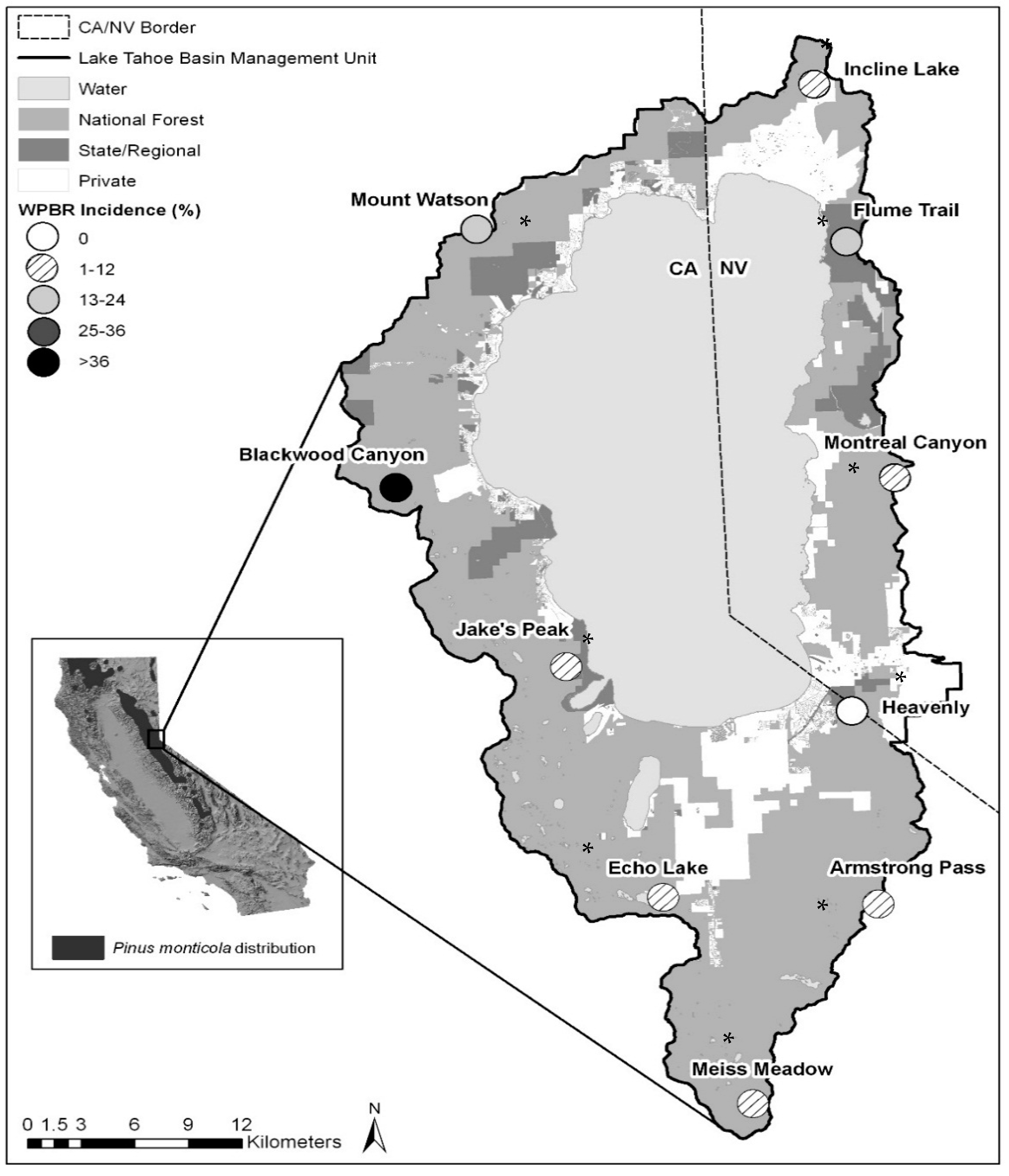
2.1. Study Area

The Lake Tahoe Basin is located in the north-central Sierra Nevada at 120° W and 39° N within the States of California and Nevada. The Basin is flanked to the west by the Sierra Nevada crest and to the east by the Carson Range, and elevations range from 1890 to 3292 m. The climate is Mediterranean and characterized by warm, dry summers and cool wet winters. Most precipitation falls as snow between the months of November and April, with a strong gradient from west to east. East-side locations are influenced by the rainshadow effect of the Sierra Nevada crest (Table 1). Geology of the region is dominated by igneous intrusive rocks, typically granodiorite, and igneous extrusive rocks, typically andesitic lahar, with small amounts of metamorphic rock [25].
In California and western Nevada, western white pine grows in mixed-species stands and is an important associate of upper montane forests at elevations ranging from 2100 m to 2900 m, but can sometimes be found up to 3300 m in the subalpine zone [26]. In the Lake Tahoe Basin several forest types occur in the upper montane, but the most dominant type is the red fir forest, with a mix of red fir (A. magnifica Andr. Murray), western white pine, lodgepole pine (P. contorta Dougl. ex. Loud.) and occasionally Jeffrey pine (P. jeffreyi Grev. & Balf.), covering approximately 5000 ha [27].
During the summer of 2008, we selected 10 study populations, with 3 permanent demographic plots per population (sampling area within a population = 4 ha), for a total of 30 plots. For our study, a population is defined as an area in which gene flow occurs (pollen and seed dispersal), which for some conifers has been estimated at about 4 hectares [28,29]. Our long-term plot network was established on National Forest System and State Park lands surrounding Lake Tahoe (Lake Tahoe Basin Management Unit/LTBMU and California and Nevada State Parks). Each of the 10 populations of western white pine was located in a distinct watershed and distributed around the Basin to capture variation in the physical environment (e.g., climate, geology, topography). For each demographic plot, annual precipitation from the period 1971–2000 was provided by FHTET (USDA FS Forest Health Technology Enterprise Team, Fort Collins, CO, USA) using the PRISM climatic model [30]. Soil survey data were provided by the South Lake Tahoe office of the USDA Natural Resources Conservation Service (NRCS). For a complete description of field methodology as well as insect and pathogen identification, see Maloney et al. [6].

2.2. Current Population Structure and Trends

Population trends were assessed with transition matrix models for each of the 10 populations of western white pine. We used transition matrices to describe and summarize current trends in survivorship, fecundity and, to a lesser extent, radial growth. Transition matrix models of populations follow the Lefkovitch [31] model. Entries in the transition matrix represent the contribution that each size class makes to every other size class during a specified time interval. We created sized-based models from six size classes: (1) recruits (individuals <1.37 m in height); (2) 0.1–5.0 cm d.b.h.; (3) 5.1–10.0 cm d.b.h.; (4) 10.1–20.0 cm d.b.h.; (5) 20.1–40.0 cm d.b.h.; and (6) ≥40.1 cm d.b.h. Transition probabilities for survival, fecundity, and growth were calculated and estimated from our field data. For growth probabilities, individuals transitioned into the next size class when they were in the upper d.b.h. limit of the size class, or of height for seedlings/saplings. For example, we assumed that an individual with a d.b.h. of 4.9–5.0 cm would grow into size class 3 in the next time step. Where mortality occurred, survival was calculated using the number of standing dead trees (years dead ranged from 1 to 12 years) divided by current live and dead stems for each size class. In demographic studies of forest trees where mortality was not observed, mortality was assumed to be 0% or 2% [4,32]. In our populations where no mortality was observed, we assumed a minimal value of 1% mortality, an average of these previously published estimates [4,32]. Fecundity was estimated from existing recruitment and cone production data for size classes 3, 4, 5, and 6 [6]. The population growth rate (λ), was estimated using the dominant eigenvalue of the transition matrix [33]. We computed 95% confidence intervals for λ by bootstrapping (n = 10,000) across survivorship, growth and fecundity estimates comprising the transition matrix. All calculations and bootstrapping were performed in Matlab [34]. Stepwise multiple linear regression was used to identify important biological and environmental variables explaining western white pine mortality in the Lake Tahoe Basin [35]. The stepwise criterion was run with forward direction with p ≤ 0.10 for variable entry. A check of collinearity in regression models was performed using leverage plots and bivariate scatterplots. Data for water use efficiency, a variable used in the multiple linear regression model, is reported in Maloney et al., (In revision).

2.3. Genetic Structure and Diversity

Within demographic plots, needle samples were taken from 25 adult western white pine individuals from each of the 10 populations in the Lake Tahoe Basin (n = 250). Sampled trees were approximately 30 m apart. Needle samples were stored in vials containing three 0.5 g desiccant packets. DNA was extracted in the laboratory from 50 mg of tissue using DNeasy® Plant 96 Kits following the manufacturer’s protocol (Qiagen, Valencia, CA, USA). DNA from sampled trees was genotyped for 384 single nucleotide polymorphisms (SNPs), which were used as genetic markers. These SNPs were discovered through resequencing of a diversity panel comprising 12 haploid megagametophytes collected across the natural range of sugar pine [36]. All genotyping was carried out at the DNA Technologies Core at the UC Davis Genome Center. Genotypes were called at each SNP locus for each tree using GenomeStudio (Illumina) software. Quality thresholds for inclusion of SNPs were the same as those given in Eckert et al. [37].
For each SNP, we calculated observed (HO) and expected (HE) heterozygosity, Wright’s inbreeding coefficient (FIS) and hierarchical F-statistics among plots nested within populations. Significance of multilocus hierarchical fixation indices was assessed using 99% bootstrap confidence intervals (CIs) (n = 10,000 replicates sampled across SNPs). We examined allelic correlations (r2) between all possible pairs of SNPs to validate our assumption that SNPs were unlinked. Analyses were conducted using the genetics and hierfstat [38] packages in R [39].
We assessed population structure using the approach outlined by Nicholson et al. [40] as implemented in the popgen library of R [39]. This approach models a set of populations that diverges instantaneously from an ancestral population. Allele frequencies in those diverging populations drift away from those in the ancestral population, and are modeled using a binomial-beta hierarchical structure [41]. Here, we used the 10 sampled populations of western white pine. There are three parameters of interest in this model: αilj, the frequency in population i at locus l of allele j; πlj, the ancestral frequency of locus l of allele j; and ci, the variance parameter for population i describing the magnitude of drift away from ancestral allele frequencies across loci. Since the ci parameters are defined in terms of variance in allele frequencies across loci, they are analogous to population-specific estimates of multilocus FST. Thus, a larger value for an estimate of the ci parameter indicates more drift away from ancestral allele frequencies, meaning that current allele frequencies within population i (αilj) are less similar, in terms of variance across loci, to those in the ancestral population (πlj). As with FST, there are no natural breaks to define easily what is high and what is low without assuming some form of equilibrium model of gene flow (e.g., island model). A comprehensive review of FST estimates for conifers is given elsewhere [42,43].
Parameters were estimated in a Bayesian framework using Markov chain Monte Carlo (MCMC), where uniform priors were placed on the ci and πlj parameters and a Metropolis-Hastings algorithm was used to sample from the posterior distribution of each parameter. The αilj parameters were integrated out of the likelihood function and thus were not sampled (cf. [40]). Markov chains were sampled 10,000 times post burn-in (n = 10,000) to estimate posterior distributions, with point estimates reported as posterior means. Convergence was assessed by comparing posterior distributions of the ci parameters across two replicated runs of the MCMC sampler, using Kolmogorov-Smirnov tests.

2.4. Evaluating Disease Resistance and Cr2 Allele Frequency

One-hundred and thirty one families (none of which exhibited symptoms of WPBR infection in field evaluations) were screened for presence of the Cr2 allele at the Placerville Nursery’s Rust Resistance Screening Program facility, Camino, CA. Western white pine seed was sown in 2009 (see Maloney et al. [6] for a complete description of culturing and screening protocols). In October 2010 (96 families) and October 2011 (35 families), test seedlings were inoculated by basidiospore casts from infected leaves of Ribes nigrum L., an alternate host to the WPBR pathogen. Ribes nigrum plants had been inoculated with uredospores derived from stored aeciospores of Cronartium ribicola collected and bulked from forested sites on the Eldorado National Forest by the Placerville Nursery, Camino, CA, USA. Seedlings with infected Ribes leaves suspended over them were incubated in dew chambers for 62 h at 17 °C and 100% relative humidity (J. Gleason, pers. comm., USDA Forest Service). In March of 2011 and 2012, the frequency of Cr2 in the western white pine family was evaluated. When challenged by C. ribicola, resistant host needles respond to infection by developing hypersensitive spots (small necrotic flecks) that prevent further fungal growth; these flecks contrast markedly with the bright yellow, expanding spots that develop on the foliage of susceptible Cr2/Cr2 genotypes [17]. Since the Cr2 allele is dominant and segregates in a 1:1 ratio of resistant to susceptible reactions, its frequency can be estimated for wind-pollinated families by counting the number of seedlings expressing the hypersensitive reaction [17]. Parents of families that segregate 1:1 resistant:susceptible are heterozygous for the Cr2 allele (genotype, Cr2Cr2). Cr2 allele frequency in a population is calculated by dividing the number of Cr2 alleles identified per family by twice the total number of families tested. Correlation analyses were conducted to determine relationships between WPBR incidence and the frequency of Cr2 and of pollen receptors (susceptible families that exhibited a very low frequency of resistant offspring, presumably derived from rare Cr2 alleles in the pollen cloud) [35].

3. Results

3.1. Western White Pine and Forest Conditions

Western white pine densities within plots ranged from a low of 56 trees·ha−1 to a high of 111 trees·ha−1 (mean = 82.5, Table 1). Basal area also varied, ranging from 5.27 m2·ha−1 to 21.9 m2·ha−1 (mean = 13.7, Table 1). White pine blister rust was found in 90% of the populations and the frequency of infected trees by population ranged from 0% to 45% (Table 1). The highest frequencies of WPBR infection were found at Blackwood Canyon (45%) and Mt Watson (23%). No rust was found on western white pine in the Heavenly population. Mountain pine beetle was found in 100% of the populations and ranged from 6% to 40% of trees infested (Table 1). High incidence of MPB was found in populations at Heavenly (40%), Flume Trail (23%), Incline Lake (17%), Armstrong Pass (17%), and Blackwood Canyon (17%) (Table 1). Western white pine mortality ranged from 2% to 17%, with the highest cumulative mortality at Heavenly and Blackwood Canyon (Table 1).
Strong environmental gradients exist within the Basin in precipitation, geology and soil type (Table 1). Mean annual precipitation is 1265 mm in west-side and 963 mm in east-side locations, respectively (Table 1). WPBR incidence is highest at Blackwood Canyon on the west-side of the Basin, which was also the most mesic location, receiving, on average, 1472 mm of precipitation annually (Table 1, Figure 1). Moist conditions are required by C. ribicola for successful infection on both hosts; all spore stages require relative humidity >90% and temperatures in the range of 15–18 °C [44,45,46]. Soil type can influence site characteristics and carrying capacity of western white pine and other forest associates (Table 1). Populations growing on decomposed granite have relatively lower densities (mean = 75 inds.·ha−1) than neighboring populations growing on volcanic or andesitic soils, which generally have higher available soil moisture (WC 15 bar mean = 7.25volcanic/andesite versus 3.8granitic), and thus support greater tree densities (mean = 94 inds.·ha−1) (Table 1).

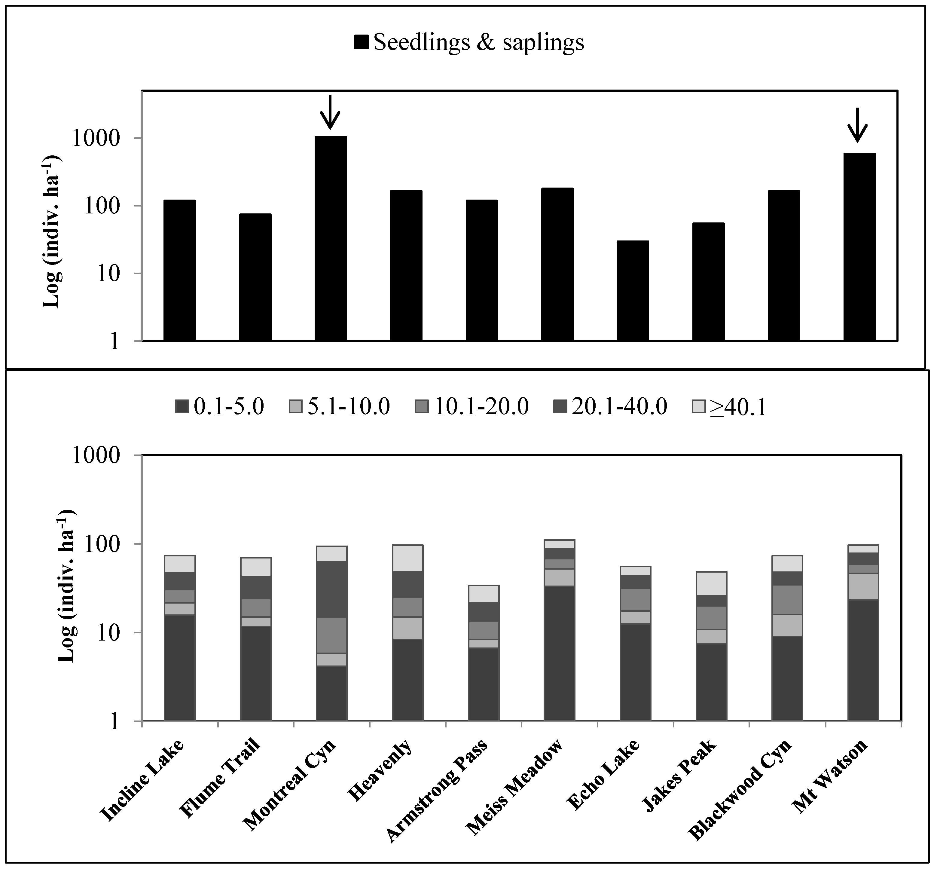
3.2. Population Structure and Trends

Multi-size structure was found for western white pine, with good representation in most size classes, particularly juveniles in the 0.1–5.0 cm diameter size class (Figure 2). High proportions of large diameter trees (>40.1 cm) were found at Incline Lake, Flume Trail, Heavenly, and Jakes (Figure 2). Relatively high numbers of seedlings and saplings were found in all populations with the greatest recruitment numbers at Montreal Canyon and Mt Watson, which also corresponds with logging activity within the last 20 years (Figure 2).
Variation in fecundity, which is a function of cone production and the number of recruits that establish successfully, was found among populations (Table 2). Fecundity was greatest at Mt Watson (1.437) and Montreal Canyon (1.036), the two locations that have been most recently logged. Low fecundity was found at Jakes Peak (0.076), Echo Lake (0.112), and Flume Trail (0.150) (Table 2). Survivorship ranged from 0.828 to 0.983 with a mean of 0.918 (Table 2). Estimated growth rates (λ) for 7 of the 10 western white pine populations were ≥1.0, indicating that these populations are apparently stable (Table 2). Blackwood Canyon (0.946), Incline Lake (0.991), and Heavenly (0.997) had λ’s <1.0, indicative of populations that may be in decline (Table 2). Because population growth, λ, was calculated from a one-time sampling, our estimates may not reflect intrinsic variation in rates of survivorship, mortality, growth, and fecundity. Our intent was not to predict future population growth but to describe current population conditions. In addition, the confidence intervals are very large for λ, which is a cause for concern, but it is difficult to assess the magnitude of this concern, as λ was estimated from a one-time sampling that likely resulted in the large variances around the point estimate.
Multiple linear regression of western white pine mortality employed 3 biotic and abiotic variables explaining 88% of the variation (model R2 = 0.88, F3,6 = 15.19, p = 0.0029). Mountain pine beetle contributed significant predictive power to the regression model, followed by CEC (cation exchange capacity, a soil property indicative of soil fertility), and water-use efficiency, δ13C (Figure 3).

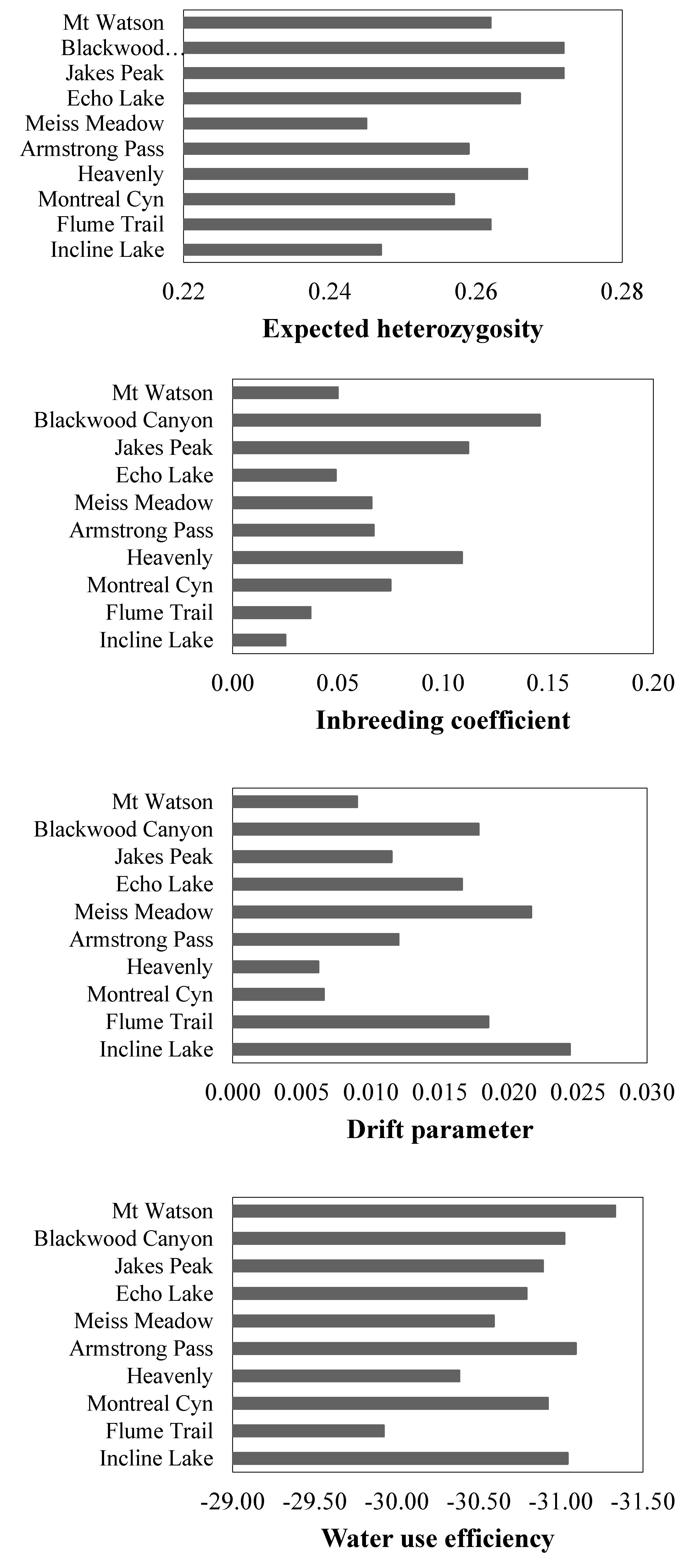
3.3. Genetic Structure and Diversity

Of the 384 SNP marker loci assessed, 160 were of high quality and segregated in our sample of 250 trees. Genetic diversity measures (HO and HE) ranged from 0.231 to 0.259, and from 0.245 to 0.272, respectively (Table 2 and Figure 4). Expected heterozygosity was similar to values reported by Kim et al. [47], derived from a limited number of samples of western white pine in California (mean HE = 0.269). The inbreeding coefficient (FIS) ranged from 0.025 to 0.146, with all populations having positive values (Table 2 and Figure 4). High positive values of FIS often indicate inbreeding, with fewer heterozygotes than expected, or within population substructure (e.g., Wahlund effect). Three populations had FIS values >0.100: Blackwood Canyon (0.146), Jakes Peak (0.112), and Heavenly (0.109). The remaining populations were within range of zero and are consistent with the Hardy-Weinberg equilibrium (Table 2).
The drift parameter (ci) ranged from 0.0062 to 0.0244 (Table 2 and Figure 4), consistent with the multilocus estimate of FST across all populations (FST = 0.0124, 99% CI: 0.0077–0.0185). Relatively low values of FST could indicate high rates of gene flow via pollen dispersal. The highest value of ci was at Incline Lake (0.0244), followed by Meiss Meadow (0.0216) (Table 2 and Figure 4). A moderate and negative relationship exists between western white pine fecundity and ci (r2 = 0.21, F1,9 = 2.19, p = 0.17). Maloney et al. [6] found a similar pattern of high genetic drift for two sugar pine populations in the Lake Tahoe Basin—likely a consequence of historical logging in the region, in both lower and upper.

3.4. Frequency of Disease Resistance

Of the 131 families (maternal parents) screened for Cr2, 4 were heterozygous for the resistance gene (Cr2Cr2), yielding an overall Cr2 allele frequency of 0.023 for sampled western white pine in the Lake Tahoe Basin. Kinloch et al. [17] reported Cr2 frequencies in the Sierra Nevada to be between 0.0046 and 0.0081 (this is because he was reporting gametic frequencies, not zygotic frequencies), nearly 3-fold lower than what we found in the Lake Tahoe Basin. Cr2 was found in 2 of 10 western white pine populations (Table 2), with zygotic frequencies of 0.07 at Meiss Meadow and 0.02 at Armstrong Pass (Table 2, Figure 1). No evidence for Cr2 was found in the remaining populations of western white pine; however, pollen receptors were identified in 9 of the 10 western white pine populations. Pollen receptors (Cr2Cr2) are susceptible female parents that conferred resistance to some of their progeny from rare R alleles in the local pollen cloud. We found a moderate and negative relationship between the frequency of pollen receptors in a population and the incidence of WPBR, r2 = 0.32, F1,9 = 3.85, p = 0.08 (Figure 5).

4. Discussion

We evaluated population and genetic characteristics of western white pine in the Lake Tahoe Basin as they relate to stand conditions, land-use, disease, and insect prevalence. Current forest conditions in our study were comparable to Taylor’s [3] findings in which he identified shifts in density, basal area, and diameter (d.b.h., diameter at breast height) in pre-Euro-American and contemporary upper montane forests of the Lake Tahoe Basin. Western white pine density was lower in pre-Euro-American upper montane forests than in contemporary forests [3] and this study (53Taylor-Pre-Euro, 71Taylor-Contemp, and 82Contemp); basal area was greater (15.5Taylor-Pre-Euro, 6.5Taylor-Contemp, and 13.68Contemp); and d.b.h. was larger (63.9Taylor-Pre-Euro, 32.1Taylor -Contemp, and 33.51Contemp) ([3], see Table 1). Taylor [3] attributes these forest structural shifts to historical logging and fire exclusion. We also documented negative population trends for three western white pine populations (Blackwood Canyon, Incline Lake, and Heavenly). These three populations, all with low estimated growth rates (λ), have moderate to high incidence of WPBR and/or MPB and some of the highest levels of mortality for western white pine. By contrast, seven populations appear to be stable (λ ≥ 1.0) because of low-to-moderate disease and insect incidence, and the presence of resistance to WPBR. Negative population trends are likely the consequence of historical land-use and altered disturbance regimes.
The effects of genetic drift can be greater when populations are small, and can act faster to reduce genetic variation. The longevity and dispersal capabilities of conifers, such as western white pine, are typically thought to counteract the effects of localized genetic drift. In the Lake Tahoe Basin, western white pine at Incline Lake had the highest drift parameter value (ci) and moderate to low population densities and low fecundity. Previously, Maloney et al. [6] found a similar pattern of high genetic drift for two sugar pine populations in the Lake Tahoe Basin—likely a consequence of historical logging in the region. Since there is clear evidence of early cut-over stands in the upper montane of the Lake Tahoe Basin, particularly in the vicinity of the Incline Lake population, historical logging may very well explain the high genetic drift within this population. Interpreting ci values requires caution, however, as any changes in local effective population sizes will affect these estimates, and they are based on a single model for population divergence (see [40]).
Much of the genetic diversity in forest tree species is found within rather than among populations [48,49]. Our landscape study reveals values of genetic diversity for western white pine similar to a rangewide study of western white pine by Kim et al. [47]. In earlier genetic studies of western white pine by Rehfeldt et al. [50] and Richardson et al. [51] found that Sierra Nevada populations had low growth potential but high cold tolerance, which may reflect the environmental conditions in the higher elevations of the Sierra Nevada, with short, dry growing seasons. The authors concluded that western white pine throughout its extensive range is a “generalist” species, with weak patterns of genetic variation among populations from a broad range of elevations [50,51]. The limitation to this conclusion, at least for California and the Sierra Nevada, is they had little representation from the Sierra Nevada (populations, n = 6).
Mountain pine beetle incidence was a significant predictor of western white pine mortality in upper montane forests of the Lake Tahoe Basin. This insect is known to preferentially attack drought-stressed trees when at low population levels [52,53,54], similar to the endemic levels we observed in the Lake Tahoe Basin. Two other predictors of mortality were cation exchange capacity and δ13C (water-use efficiency). We found that mortality was higher on soils with larger values of CEC, indicative of non-granitic soil types (e.g., volcanic), and in populations of western white pine with phenotypic means for δ13C having more negative values, as found on volcanic soil types (the more negative the value the less water-use efficient). In summary, for the Lake Tahoe Basin, western white pine mortality is associated with important biotic agents such as MPB and WPBR and with soil properties, particularly as related to traits such as water-use efficiency.
Moderate to high levels of infection by C. ribicola were found on western white pine in the Lake Tahoe Basin. The major gene for resistance, Cr2, was identified in only two populations; but pollen receptors (rare resistance alleles in the pollen cloud that pollinated non-Cr2 parent trees) were found in nine of the 10 populations. Blackwood Canyon was the one population with no evidence of pollen receptors and was the population with the highest levels of WPBR infection in this study (45%) (see Figure 4). Cr2 frequencies in the Lake Tahoe Basin were nearly three-fold higher than what Kinloch et al. [17] reported.

5. Conclusions

Upper montane forests provide significant biological and hydrological functions and services, including biodiversity, high carbon storage, and deep and long-lasting snowpacks [55,56,57]. In the context of fire suppression, an introduced pathogen, prolonged droughts, and catastrophic wildfires, conservation and management strategies appear to be warranted for this important species and forest type. As in lower elevation forests, restoration treatments that mitigate fire and drought may be appropriate for some locations in the upper montane [58,59]. Similar to Taylor [3], recommendations to reintroduce fire appear necessary if forest conditions allow, to promote natural western white pine regeneration. Without management action, catastrophic wildfires, infection by WPBR, and elevated MPB activity in this forest type may cause significant ecological (e.g., reduced population sizes), environmental (e.g., greater fuels, carbon loss), and genetic losses, including loss of naturally occurring resistance to WPBR, already present in western white pine. Rangewide seed collections and screening for Cr2 are needed for western white pine in California. Such efforts will be needed to enhance collections of rust-resistant western white pine as well as provide a local and diverse seed source for post-wildfire restoration and post-MPB outbreak recovery.

Acknowledgments

We thank Tom Burt for field assistance and cone collections and Akiko Aguchi for GIS maps. We also thank Joan Dunlap, John Gleason, and Dessa Welty, USDA Forest Service, Sugar Pine Rust Resistance Program, Placerville Nursery, for processing western white pine cones and seed, seed-banking, and screening for Cr2. Jill Wegrzyn for bioinformatics and Katie Tsang for DNA extraction. David Fournier (USDA Forest Service, LTBMU), Roland Shaw (Nevada Division of Forestry), Woody Loftis (USDA, NRCS), Bill Champion (Nevada State Parks), and Audrey Newman (Heavenly Mountain Resort) for site information and permission to work on Federal, State, and private lands. Our work was supported by the Southern Nevada Public Lands Management Act—Rounds 7 and 9, which were sponsored by the USDA Forest Service, Pacific Southwest Research Station, Albany, CA.

Author Contributions

P.E.M., A.J.E., D.R.V., A.D.M., and D.B.N. designed the study. P.E.M., A.J.E., D.R.V., and C.E.J. were responsible for the data collection and data analysis. P.E.M., A.J.E., and D.R.V. led the writing of the manuscript with contributions from C.E.J., A.D.M., and D.B.N.

Conflicts of Interest

The authors declare no conflict of interest.

References

  1. Laudenslayer, W.F.J.; Darr, H.H. Historical effects of logging on the forests of the Cascade and Sierra Nevada ranges in California. Trans. West. Sect. Wild. Soc. 1990, 26, 12–23. [Google Scholar]
  2. Fins, L.; Byler, J.; Ferguson, D.; Harvey, A.; Mahalovich, M.F.; McDonald, G.; Miller, D.; Schwandt, J.; Zack, A. Return of the giants: Restoring western white pine to the inland Northwest. J. For. 2002, 100, 20–26. [Google Scholar]
  3. Taylor, A.H. Identifying forest reference conditions on early cut-over lands of the Lake Tahoe Basin, USA. Ecol. Appl. 2004, 14, 1903–1920. [Google Scholar] [CrossRef]
  4. Van Mantgem, P.J.; Stephenson, N.L.; Keifer, M.; Keeley, J. Effects of an introduced pathogen and fire exclusion on the demography of sugar pine. Ecol. Appl. 2004, 14, 1590–1602. [Google Scholar] [CrossRef]
  5. Shaw, C.G.; Geils, B.W. Special Issue: White Pines, Ribes, and Blister Rust. For. Pathol. 2010, 40, 145–418. [Google Scholar] [CrossRef]
  6. Maloney, P.E.; Vogler, D.R.; Eckert, A.J.; Jensen, C.E.; Neale, D.B. Population biology of sugar pine (Pinus lambertiana Dougl.) with reference to historical disturbances in the Lake Tahoe Basin: Implications for restoration. For. Ecol. Manag. 2011, 262, 770–779. [Google Scholar] [CrossRef]
  7. Goheen, E.M.; Goheen, D.J. Status of Sugar and Western White Pines on Federal Forest Lands in Southwest Oregon: Inventory Query and Natural Stand Survey Results; Report No. SWOFIDSC-14-01; USDA Forest Service, Pacific Northwest Region: Portland, OR, USA, 2014; p. 71. [Google Scholar]
  8. Gernandt, D.S.; Geada López, G.; Ortiz García, S.; Liston, A. Phylogeny and classification of Pinus. Taxon 2005, 54, 29–42. [Google Scholar] [CrossRef]
  9. Sudworth, J.B. Unpublished Field Note Books of Sierra Nevada Forest Reserve Inventory; University of California, Berkeley, Bioscience and Natural Resources Library: Berkeley, CA, USA, 1899. [Google Scholar]
  10. McKelvey, K.S.; Johnston, J.D. Historical perspectives on forests of the Sierra Nevada and the Transverse Ranges of southern California: Forest conditions at the turn of the century. General Technical Report; GTR-PSW-133; Verner, J., McKelvey, K.S., Noon, B.R., Gutierrez, R.J., Gould, G.I.J., Beck, T.W., Eds.; Tech. Coords., U.S. Forest Service, Pacific Southwest Research Station: Albany, CA, USA, 1992; pp. 225–246. [Google Scholar]
  11. Ansley, J.; Battles, J.J. Forest composition, structure, and change in an old-growth mixed conifer forest in the northern Sierra Nevada. J. Torr. Bot. Soc. 1998, 125, 297–308. [Google Scholar] [CrossRef]
  12. Stephens, S.L. Mixed conifer and red fir forest structure and uses in 1899 from the central and northern Sierra Nevada, California. Madroño 2000, 47, 43–52. [Google Scholar]
  13. Maloney, P.E. Incidence and distribution of white pine blister rust in the high-elevation forests of California. For. Pathol. 2011, 41, 308–316. [Google Scholar] [CrossRef]
  14. Homans, G.M. Seventh Biennial Report of the State Board of Forestry of the State of California; California State Printing Office: Sacramento, CA, USA, 1919. [Google Scholar]
  15. Neuenschwander, L.F.; Byler, J.W.; Harvey, A.E.; McDonald, G.I.; Ortiz, D.S.; Osborne, H.L.; Snyder, G.C.; Zack, A. White Pine in the American West: A Vanishing Species-Can We Save It? General Technical Report; RMRS-GTR-35; U.S. Department of Agriculture, Forest Service, Rocky Mountain Research Station: Ogden, UT, USA, 1999; p. 20. [Google Scholar]
  16. Smith, R.S. Spread and intensification of blister rust in the range of sugar pine. In Sugar Pine: Status, Values, and Roles in Ecosystems: Proceedings of a Symposium presented by the California Sugar Pine Management; Publication 3362; Kinloch, B.B.J., Marosy, M., Huddleston, M.E., Eds.; University of California, Division of Agriculture and Natural Resources: Davis, CA, USA, 1996; pp. 112–118. [Google Scholar]
  17. Kinloch, B.B.J.; Sniezko, R.A.; Dupper, G.E. Origin and distribution of Cr2, a gene for resistance to white pine blister rust in natural populations of western white pine. Phytopatologyh 2003, 93, 691–694. [Google Scholar] [CrossRef] [PubMed]
  18. Kinloch, B.B.J.; Littlefield, J.L. White pine blister rust: Hypersensitive resistance in sugar pine. Can. J. Bot. 1976, 55, 1148–1155. [Google Scholar] [CrossRef]
  19. Taylor, A.H.; Halpern, C.B. The structure and dynamics of Abies magnifica forests in the southern Cascade Range, USA. J. Veg. Sci. 1991, 2, 189–200. [Google Scholar] [CrossRef]
  20. Taylor, A.H. Fire history and structure of red fir (Abies magnifica) forests, Swain Mountain Experimental Forest, Cascade Range, northeastern California. Can. J. For. Res. 1993, 23, 1672–1678. [Google Scholar] [CrossRef]
  21. Stephens, S.L. Fire history differences in adjacent Jeffrey pine and upper montane forests in the eastern Sierra Nevada. Int. J. Wildland Fire 2001, 10, 161–167. [Google Scholar] [CrossRef]
  22. North, M.P.; van de Water, K.M.; Stephens, S.L.; Collins, B.M. Climate, rain shadow, and human-use influences on fire regimes in the eastern Sierra Nevada, California, USA. Fire Ecol. 2009, 5, 20–34. [Google Scholar] [CrossRef]
  23. Perry, D.A.; Hessburg, P.; Skinner, C.N.; Spies, T.A.; Stephens, S.L.; Taylor, A.H.; Franklin, J.; McComb, B.; Riegel, G. The ecology of mixed severity fire regimes in Washington, Oregon, and Northern California. For. Ecol. Manag. 2011, 262, 703–717. [Google Scholar] [CrossRef]
  24. Meyer, M.D. Natural Range of Variation of Subalpine Forests in the Bioregional Assessment Area; Unpublished Report; USDA Forest Service, Pacific Southwest Region: Vallejo, CA, USA, 2013. [Google Scholar]
  25. Unites States Department of Agriculture, Natural Resources Conservation Service. Soil Survey of the Tahoe Basin Area, California and Nevada; USDA NRCS: Washington, DC, USA, 2007. [Google Scholar]
  26. Kinloch, B.B.J.; Scheuner, W.H. Pinus lambertiana Dougl., sugar pine. In Silvics of North America; Burns, R.M., Honkala, B.H., Eds.; USDA Forest Service: Washington, DC, USA, 1990; pp. 370–379. [Google Scholar]
  27. Manley, P.N.; Fites-Kaufman, J.A.; Barbour, M.G.; Schlesinger, M.D.; Rizzo, D.M. Biological Integrity. In Lake Tahoe Basin Watershed Assessment, Volume 1; Gen. Tech. Rep. PSW-GTR-175; Murphy, D.D., Knopp, C.M., Eds.; Pacific Southwest Research Station, USDA Forest Service: Albany, CA, USA, 2000; pp. 403–600. [Google Scholar]
  28. Neale, D.B. Population Genetic Structure of the Douglas-Fir Shelterwood Regeneration System in Southwest Oregon. Ph.D. Dissertation, Oregon State University, Corvallis, OR, USA, 1983. [Google Scholar]
  29. Adams, W.T.; Birkes, D.S. Estimating mating patterns in forest tree populations. In Proceedings of the International Workshop on Plant Biology, Biochemical Markers in Population Genetics of Forest Trees, Porano-Orvieto, Italy, 11–13 October 1988; Hattemer, H.H., Fineschi, S., Eds.; Institute of Agroforestry and Natural Resources Council Italy (CNR), SPB Academic Publishing: The Hague, The Netherlands, 1990; pp. 152–172. [Google Scholar]
  30. Daly, C.; Neilson, R.P.; Phillips, D.L. A statistical model for mapping climatological precipitation over mountainous terrain. J. Appl. Meteorol. 1994, 33, 140–158. [Google Scholar] [CrossRef]
  31. Lefkovitch, L.P. The study of population growth in organisms grouped by stage. Biometrics 1965, 21, 1–18. [Google Scholar] [CrossRef]
  32. Ettl, G.J.; Cottone, N. Whitebark pine (Pinus albicaulis) in Mt. Rainier National Park, Washington, USA: Response to blister rust infection. In RAMAS GIS; Akçakaya, H.R., Ed.; Applied Mathematics: Setauket, NY, USA; New York, NY, USA, 2002; pp. 36–48. [Google Scholar]
  33. Caswell, H. Matrix Population Models, 2nd ed.; Sinauer Associates: Sunderland, MA, USA, 2001. [Google Scholar]
  34. MATLAB; The Mathworks, Inc.: 3 Apple Hill Dr., Natick, MA, USA, 2009.
  35. SAS Institute. JMP Start Statistics: JMP Statistics and Graphics Guide; release 8.0.1; SAS Institute Inc.: Cary, NC, USA, 2009. [Google Scholar]
  36. Jermstad, K.D.; Eckert, A.J.; Wegrzyn, J.L.; Mix, A.D.; Davis, D.A.; Burton, D.C.; Neale, D.B. Comparative mapping in Pinus: Sugar pine (Pinus lambertiana Dougl.) and loblolly pine (Pinus taeda). Tree Gen. Genom. 2011, 7, 457–468. [Google Scholar] [CrossRef]
  37. Eckert, A.J.; Ersoz, E.S.; Pande, B.; Wright, M.H.; Rashbrook, V.K.; Nicolet, C.M.; Neale, D.B. High-throughput genotyping and mapping of single nucleotide polymorphisms in loblolly pine (Pinus taeda L.). Tree Gen. Genom. 2009, 5, 225–234. [Google Scholar] [CrossRef]
  38. Goudet, J. Hierfstat, a package for R to compute and test hierarchical F-statistics. Mol. Ecol. Notes 2005, 5, 184–186. [Google Scholar] [CrossRef]
  39. R Development Core Team. R: A language and environment for statistical computing. R Foundation for Statistical Computing. Vienna, Austria. Available online: http://www.R-project.org (accessed on 15 January 2007).
  40. Nicholson, G.; Smith, A.V.; Jonsson, F.; Gustafsson, O.; Stefansson, K.; Donnelly, P. Assessing population differentiation and isolation from single-nucleotide polymorphism data. J. R. Stat. Soc. B 2002, 64, 695–715. [Google Scholar] [CrossRef]
  41. Balding, D.; Nichols, R. A method for quantifying differentiation between populations at multi-allelic loci and its implications for investigating identity and paternity. Genetica 1995, 96, 3–12. [Google Scholar] [CrossRef] [PubMed]
  42. Ledig, F.T. Genetic variation in Pinus. In Ecology and Biogeography of Pinus; Richardson, D.M., Ed.; Cambridge University Press: Cambridge, UK, 1990; pp. 251–280. [Google Scholar]
  43. Savolainen, O.; Pyhäjärvi, T.; Knürr, T. Gene flow and local adaptation in forest trees. Annu. Rev. Ecol. Evol. Systemat. 2007, 38, 595–619. [Google Scholar] [CrossRef]
  44. Hirt, R.R. The Relation of Certain Meterological Factors to the Infection of Eastern White Pine by the Blister-Rust Fungus; Tech. Pub. No. 59; The New York State College of Forestry, Syracuse University: Syracuse, NY, USA, 1942. [Google Scholar]
  45. Van Arsdel, E.P.; Riker, A.J.; Patton, R.F. The effects of temperature and moisture on the spread of white pine blister rust. Phytopathology 1956, 6, 307–318. [Google Scholar]
  46. McDonald, G.I. Ecotypes of blister rust and management of sugar pine in California. In Sugar Pine: Status, Values, and Roles in Ecosystems; Publication 3362; Proceedings of a Symposium presented by the California Sugar Pine Management, Davis, CA, USA, 30 March–1 April 1992; Kinloch, B.B.J., Marosy, M., Huddleston, M.E., Eds.; University of California, Division of Agriculture and Natural Resources: Davis, CA, USA, 1996; pp. 137–147. [Google Scholar]
  47. Kim, M.-S.; Richardson, B.A.; McDonald, G.I.; Klopfenstein, N.B. Genetic diversity and structure of western white pine (Pinus monticola) in North America: A baseline study for conservation, restoration, and addressing impacts of climate change. Tree Gen. Genom. 2011, 7, 11–21. [Google Scholar] [CrossRef]
  48. Hamrick, J.L.; Godt, M.J.W. Conservation genetics of endemic plant species. In Conservation Genetics: Case Histories from Nature; Avise, J.C., Hamrick, J.L., Eds.; Chapman & Hall: New York, NY, USA, 1996; pp. 281–304. [Google Scholar]
  49. Hamrick, J.L. Response of forest trees to global environmental changes. For. Ecol. Manag. 2004, 197, 323–335. [Google Scholar] [CrossRef]
  50. Rehfeldt, G.E.; Hoff, R.J.; Steinhoff, R.J. Geographic patterns of genetic variation in Pinus monitcola. Bot. Gaz. 1984, 145, 229–239. [Google Scholar] [CrossRef]
  51. Richardson, B.A.; Rehfeldt, G.E.; Kim, M.-S. Congruent climate-related genecological responses from molecular markers and quantitative traits for western white pine (Pinus monticola). Int. J. Plant Sci. 2009, 170, 1120–1131. [Google Scholar] [CrossRef]
  52. Breshears, D.D.; Cobb, N.S.; Rich, P.M.; Price, K.P.; Allen, C.D.; Balice, R.G.; Romme, W.H.; Kastens, J.H.; Floyd, M.L.; Belnap, J.; et al. Regional vegetation die-off in response to global-change-type drought. Proc. Natl. Acad. Sci. USA 2005, 102, 15144–15148. [Google Scholar] [CrossRef] [PubMed]
  53. Bentz, B.J.; Régnière, J.; Fettig, C.J.; Hansen, E.M.; Hicke, J.; Hayes, J.L.; Kelsey, R.; Negrón, J.; Seybold, S.J. Climate change and bark beetles of the western US and Canada: Direct and indirect effects. BioScience 2010, 60, 602–613. [Google Scholar] [CrossRef]
  54. Boone, C.K.; Aukema, B.H.; Bohlman, J.; Carroll, A.L.; Raffa, K.F. Efficacy of tree defense physiology varies with bark beetle population density: A basis for positive feedback in eruptive species. Can. J. For. Res. 2011, 41, 1174–1188. [Google Scholar] [CrossRef]
  55. Barbour, M.G.; Minnich, R.A. California upland forests and woodlands. In North American Terrestrial Vegetation; Barbour, M.G., Billings, W.D., Eds.; Cambridge University Press: New York, NY, USA, 2000; pp. 161–202. [Google Scholar]
  56. SNEP Science Team. Status of the Sierra Nevada: Final Report to Congress of the Sierra Nevada Ecosystem Project; 3 Volume, Rep 36; Wildland Resources Center, University of California: Davis, CA, USA, 1996. [Google Scholar]
  57. Stephenson, N.L.; Das, A.J.; Condit, R.; Russo, S.E.; Baker, P.J.; Beckman, N.G.; Coomes, D.A.; Lines, E.R.; Morris, W.K.; Rüger, N.; et al. Rate of tree carbon accumulation increases continuously with tree size. Nature 2014, 507, 90–93. [Google Scholar] [CrossRef] [PubMed]
  58. Stephens, S.L.; Ruth, L.W. Federal forest fire policy in the United States. Ecol. Appl. 2005, 15, 532–542. [Google Scholar] [CrossRef]
  59. Stephens, S.L.; Agee, J.; Fulé, P.; North, M.; Romme, W.; Swetnam, T.; Turner, M. Managing forests and fire in changing climates. Science 2013, 342, 41–42. [Google Scholar] [CrossRef] [PubMed]
Figure 1. Location of study area and western white pine plots in the Lake Tahoe Basin. Pinus monticola distribution in California is shown in insert (distribution map source USGS 1999 Digital representation of ‘‘Atlas of United States Trees’’ by Elbert L. Little, Jr.). Populations with Cr2 are noted and asterisks indicate populations where pollen receptors are present.
Forests 07 00093 g001
Figure 2. Seedling and sapling abundance and size structure for ten population of western white pine in the Lake Basin. Population structure is represented by stems in d.b.h. size classes 0.1–5.0 cm, 5.1–10.0 cm, 10.1–20.0 cm, 20.1–4.0 cm, and ≥40.1 cm. Arrows denote populations that were recently logged.
Forests 07 00093 g002
Figure 3. Multiple linear regression of western white pine mortality employed three biotic and abiotic variables explaining 88% of the variation (model R2 = 0.88, F3,6 = 15.19, p = 0.0029). Mountain pine beetle contributed a significant amount of predictive power to the regression model (A), followed by CEC (B), and water-use efficiency, δ13C (C).
Forests 07 00093 g003aForests 07 00093 g003b
Figure 4. Genetic and trait patterns for western white pine populations from the Lake Tahoe Basin.
Forests 07 00093 g004aForests 07 00093 g004b
Figure 5. Moderate and negative relationship between the incidence of WPBR and frequency of pollen receptors in a population. Blackwood Canyon is denoted by the arrow.
Forests 07 00093 g005
Table 1. Biological and environmental summaries for 10 populations of Pinus monticola in the Lake Tahoe Basin. Stands are listed clockwise in orientation in the Lake Tahoe Basin from north, east, south, and west. d.b.h. (cm) (diameter at breast height); % WPBR (white pine blister rust) = % incidence of WPBR; % MPB (mountain pine beetle) = % incidence of MPB; Elev. = elevation above sea level/a.s.l. (m); Ann. ppt. = total annual precipitation in millimeters (mm); Tmin (°C) = minimum January temperature; Tmax (°C) = maximum July temperature; WC 15 bar = soil water capacity at 15 bar; % sand = percentage sand content (sand:silt:clay); CEC = cation exchange capacity. See Methods for sources of climate and soil survey data.
LocationDensity (inds. ha−1)Basal Area (m2 ha−1)d.b.h. (cm)WPBR (%)MPB (%) Mortality (%) ElevAnn pptTmin (°C)Tmax (°C)WC 15 barSand (%) CECSoil Type
Incline Lake7421.938.81017925781394−7.621.93.479.02.9G
Flume Trail709.2732.0132352414797−7.823.43.884.91.9G
Montreal Cyn9411.635.6915122439710−6.824.310.234.722.5M
Heavenly9718.341.3040172503815−7.422.53.181.01.9G
Armstrong Pass7619.138.2417626751100−9.021.65.590.62.9G
Meiss Meadow11114.624.846226871310−8.321.33.666.212.5A, TB
Echo Lake565.2724.666422921292−6.623.01.684.01.67G
Jakes Peak7614.840.0111223701218−6.822.75.5786.92.6G
Blackwood Cyn7414.939.445171721551472−6.723.17.866.125.9TL, V
Mt Watson977.120.4239724131035−7.223.77.466.016.3A
Notes: Soil type abbreviations: A = andesite; G = granite; M = metamorphic; TB = tuff breccia; TL = tuff lahar; V = volcanic.
Table 2. Demographic and genetic summaries for P. monticola populations from the Lake Tahoe Basin. Mean fecundity, survival (cumulative mortality in bold and parentheses below), and population growth rate (λ along with 2.5% and 97.5% confidence intervals) from transition matrices. Genetic and diversity patterns from 160 marker loci with mean and variance (in parentheses) for HO, HE, FIS, ci, with 95% credible intervals for ci (in parentheses), Cr2 allele frequency, and mean water-use efficiency, δ13C.
PopulationFecunditySurvivalλHOHEFISciCr2δ13C
Incline Lake0.2070.9120.9910.2440.2470.0250.02440.00−31.04
(0.09)(0.502, 1.625)(0.038)(0.031)(0.048)(0.0149–0.0362)
Flume Trail0.1500.9491.0240.253 0.2620.0370.01850.00−29.92
(0.05)(0.667, 1.550)(0.039)(0.032)(0.055)(0.0096–0.0296)
Montreal Cyn1.0360.8801.0010.2380.2570.0750.00660.07−30.92
(0.12)(0.494, 1.639)(0.034)(0.031)(0.066)(0.0008–0.0144)
Heavenly0.2110.8280.9970.2350.2670.1090.00620.00−30.38
(0.17)(0.315, 1.719)(0.030)(0.030)(0.070)(0.0009–0.0138)
Armstrong Pass0.2020.9361.0110.2430.2590.0670.01200.02−31.09
(0.06)(0.753, 1.517)(0.036)(0.031)(0.058)(0.0049–0.0210)
Meiss Meadow0.3570.9791.0730.2310.2450.0660.02160.00−30.59
(0.02)(0.693, 1.545)(0.034)(0.031)(0.061)(0.0124–0.0332)
Echo Lake0.1120.9581.0560.2590.2660.0490.01660.00−30.79
(0.04)(0.760, 1.461)(0.041)(0.030)(0.067)(0.0088–0.0260)
Jakes Peak0.0760.9831.0610.2520.2720.1120.01150.00−30.89
(0.02)(0.784, 1.470)(0.035)(0.026)(0.094)(0.0053–0.0189)
Blackwood Cyn0.2630.8330.9460.2440.2720.1460.01780.00−31.02
(0.17)(0.679, 1.539)(0.038)(0.031)(0.091)(0.009–0.272)
Mt Watson1.4370.9291.0050.2530.2620.0500.00900.00−31.33
(0.07)(0.653, 1.779)(0.036)(0.029)(0.068)(0.0024–0.0176)

