Cross-Correlation of Diameter Measures for the Co-Registration of Forest Inventory Plots with Airborne Laser Scanning Data

Abstract

Continuous maps of forest parameters can be derived from airborne laser scanning (ALS) remote sensing data. A prediction model is calibrated between local point cloud statistics and forest parameters measured on field plots. Unfortunately, inaccurate positioning of field measures lead to a bad matching of forest measures with remote sensing data. The potential of using tree diameter and position measures in cross-correlation with ALS data to improve co-registration is evaluated. The influence of the correction on ALS models is assessed by comparing the accuracy of basal area prediction models calibrated or validated with or without the corrected positions. In a coniferous, uneven-aged forest with high density ALS data and low positioning precision, the algorithm co-registers 91% of plots within two meters from the operator location when at least the five largest trees are used in the analysis. The new coordinates slightly improve the prediction models and allow a better estimation of their accuracy. In a forest with various stand structures and species, lower ALS density and differential Global Navigation Satellite System measurements, position correction turns out to have only a limited impact on prediction models.

1. Introduction

Traditional forest inventory practices mainly rely on statistical descriptions obtained from field sample plots [1]. This method provides reliable estimates at the forest level, while limiting fieldwork cost.

However, information at the management unit level (compartment) is often not usable, due to the low number of observations. In the past decade, airborne laser scanning (ALS) has demonstrated its ability to model the 3D geometrical structure of the canopy, even at the single tree level. The area-based approach aims at combining the high resolution of ALS data with the sample field plots in order to provide statistically calibrated, continuous maps of forest parameters [2,3]. Relationships between local descriptors of the ALS point cloud and forest parameters, such as basal area, stem volume or dominant height, are investigated based on the available field data. Once a prediction model is validated, it is applied to the whole ALS dataset in order to produce the map of the desired forest parameters.

Whereas the planimetric accuracy of an ALS point cloud is around 25 cm [4], the position accuracy of field plots is lower. Indeed, plots are generally positioned relatively to elements that are visible on aerial pictures or with Global Navigation Satellite System (GNSS) receivers. Because of the canopy that reflects and attenuates the signal, the accuracy of measurements inside forest stands is lower than in open areas and of the order of a few meters [5]. However, position accuracy is difficult to estimate, as it depends on acquisition parameters, satellite availability and canopy density. Moreover, precision values provided by post-processing software cannot be considered as reliable indicators [6].

A proper co-registration is particularly important when field observations are linked to remote sensing data [7]. With ALS data, when the GNSS positions are shifted from the field positions, the predictive relationships are investigated between point clouds that do not exactly correspond to the inventoried sample plots. This error is likely to decrease the degree of fit of the final prediction models [8,9] and also result in a bad assessment of the prediction accuracy.

Several methods have been proposed to improve the co-registration of forest field plots with remote sensing data. Korpela et al. [7] used field triangulation and points derived from photogrammetry to improve the absolute mapping of large forest plots. Their method can be implemented by a single person with real-time estimation of positioning accuracy on the field. Hauglin et al. [10] co-register field plots by matching trees detected in ALS data with trees detected in terrestrial laser scanning data. When the relative tree position is recorded for the field plots and ALS with a sufficient pulse density is available, a visual comparison of the canopy height model (CHM) with the trees position and size is possible. However this task is time-consuming, in particular when the position error is large or when the forest canopy is closed and homogeneous. Some methods aim at automatically adjusting the tree position to ALS data. Olofsson et al. [11] first detected single trees in the CHM and then computed single trees position images with trees modeled as Gaussian surfaces. The image of the field trees is cross-correlated with the image of the detected trees in order to estimate the shift to be applied to the initial position. High co-registration accuracies are obtained, provided that the position error of single trees is small. This approach relies on single tree detection, which requires high density ALS data [12]. Dorigo et al. [13] define a cost function that takes into account the difference in field and CHM heights, as well as the social status of a tree. Pascual et al. [14] also take into account the match between the ALS digital terrain model and topographic measurements. Some limitations are that these methods rely on single tree detection, which might be difficult in the case of low ALS density, or on height field measures, which are generally measured only for a sample of trees. An alternative would be to use the values of the diameter, which is the most common dendrometric measure and is highly correlated with tree height.

The main objective of this article is to investigate whether the diameter information suffices for co-registration and to evaluate the sensitivity to the number of georeferenced trees. Results obtained with diameter will also be compared to those obtained with height, either with cross-correlation or by adapting the cost function based on the difference between field and CHM heights [13]. The secondary objective is to evaluate to what extent the co-registration affects the assessment of the accuracy of ALS prediction models. The whole workflow is tested on two datasets with different forest structures and ALS pulse densities.

2. Material

2.1. Study Areas

The first study area is the public forest of Prénovel and Les Piards (Jura, France, Figure 1). The elevation range is narrow (900 to 1060 m), but the topography is rough. The forest is mainly constituted of uneven-aged, mixed stands of silver fir (Abies alba), Norway spruce (Picea abies) and beech (Fagus sylvatica). Permanent sample plots were installed in 2005, and the inventory was updated between 9 September and 6 October 2011. The sampling design is a grid pattern of a size of 200 m × 200 m, which results in 139 plots inside the forest (583 ha). Plot centers were positioned with a recreational-grade GNSS receiver. On each plot, all trees with a diameter at breast height (DBH) above 7.5 cm were inventoried up to a radius of 10 m and all trees with a DBH above 27.5 cm up to 17 m. For each tree, the azimuth and distance from the plot center, the DBH and species were recorded. Forest statistics are displayed in Table 1.

Figure 1. Location of the study areas and the positions of forest inventory plots.

Figure 1. Location of the study areas and the positions of forest inventory plots.

Table 1. Forest statistics for the two study areas. The means ± standard deviations are on the first line, minimum–maximum values are on the second one.

Study area	Dominant height (m)	Basal area (m2·ha−1)	Coniferous proportion weighted by basal area	Stem density (ha−1)	Mean diameter (cm)
Jura		31.8 ± 9.2	0.87 ± 0.12	510 ± 150	25.8 ± 7.0
np = 139		13.3 − 60.5	0.49 − 1.0	110 − 1, 520	14.8 − 54.5
Vosges	23.9 ± 7.0	40.7 ± 9.2	0.53 ± 0.38	1, 990 ± 2, 900	20.8 ± 11.5
np = 95	7.6 − 38.4	10.8 − 75.2	0 − 1	170 − 17, 700	2.4 − 51.5

Table 1. Forest statistics for the two study areas. The means ± standard deviations are on the first line, minimum–maximum values are on the second one.

Study area	Dominant height (m)	Basal area (m2·ha−1)	Coniferous proportion weighted by basal area	Stem density (ha−1)	Mean diameter (cm)
Jura		31.8 ± 9.2	0.87 ± 0.12	510 ± 150	25.8 ± 7.0
np = 139		13.3 − 60.5	0.49 − 1.0	110 − 1, 520	14.8 − 54.5
Vosges	23.9 ± 7.0	40.7 ± 9.2	0.53 ± 0.38	1, 990 ± 2, 900	20.8 ± 11.5
np = 95	7.6 − 38.4	10.8 − 75.2	0 − 1	170 − 17, 700	2.4 − 51.5

The second study area is located in the department of Haut-Rhin (France), in the Vosges mountains (Figure 1). The elevation range is 200 to 1424 m. Ninety five plots were inventoried between 12 December 2011, and 19 April 2012. The sampling was designed to distribute plots into several environmental categories, including slope, site quality and forest stand type. The distribution of plots in stand development categories was: 14 young stands, 35 active growth stands, 29 mature stands and 17 uneven-aged stands. Plots are distributed equally into the poor and rich site quality categories and in the broadleaved, mixed and coniferous categories. Plot center positions were acquired with a survey-grade GNSS receiver during at least 15 min and post-processed for differential correction. All trees higher than 1.3 m and within 6 m from the plot center were inventoried. Trees with a DBH above 17.5 cm were inventoried up to a 15-m horizontal distance. For each tree, the DBH, azimuth and distance from the plot center were measured. The heights of the six trees with the largest diameters were also recorded. The main encountered species were silver fir (30% of basal area), beech (23%) and Norway spruce (18%).

2.2. Airborne Laser Scanning Data

In the Jura study area, the flight took place in leaf-on conditions, from 16–17 September 2012, with a full waveform RIEGL LMS-Q560 scanner on a fixed-wing aircraft. The flight speed was 180 km·h⁻¹ at 500 m above the ground, with a strip overlap of 60%. The pulse frequency was 180 kHz with a scan angle of ±30 degrees. The obtained mean pulse density on the 9.2 km² was 9.3 m⁻². Pre-processing of the raw files was done by the contractor. Echoes were extracted and georeferenced with the RIEGL software suite. The resulting point cloud was classified into two classes (ground and vegetation) with TerraScan. The pulse density on the field plots ranges from 6.3 to 14.1 m⁻².

In the Vosges study area, airborne laser scanning data were acquired by the French Institute of Geographical and Forest Information during March and April 2011. Vegetation was mainly in leaf-off condition, and snow remained on the ground in some high areas. The scanner was an Optech ALTM3100 mounted on a fixed-wing aircraft flying at 290 km·h⁻¹ at 1500 m above the ground. The pulse frequency was 71 kHz with a scan angle of ±16 degrees. The obtained mean pulse density on the 1362 km² was 2.6 m⁻². TerraScan was used for echo classification in ground and non-ground categories. The pulse density on the field plots ranges from 1.1 to 4.1 m⁻².

3. Methods

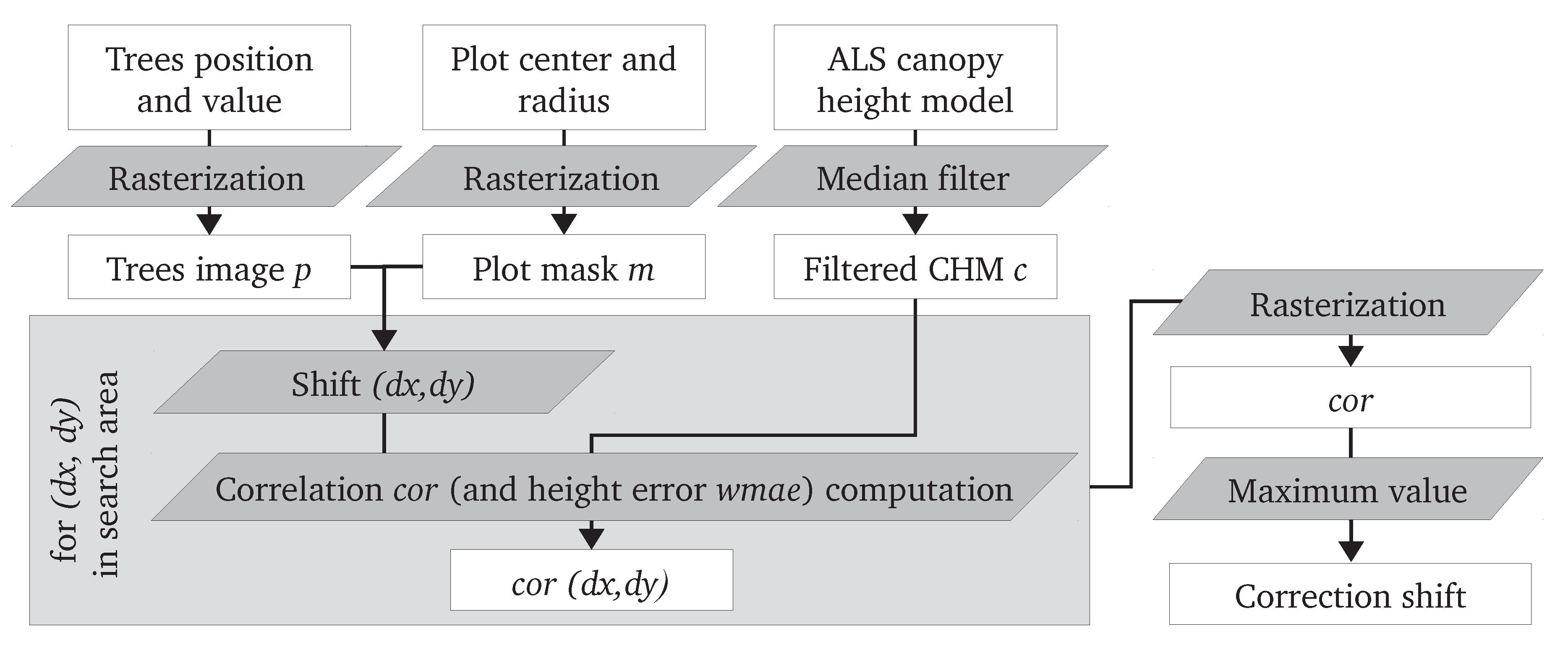
3.1. Co-Registration Algorithm

The workflow for the co-registration of a plot is presented in Figure 2. The required inputs are: trees position and value (diameter or height), plot center position and radius and the canopy height model (CHM). The CHM is the difference between the digital surface model, calculated by retaining the altitude of the highest ALS point in each pixel, and the digital terrain model, calculated by bilinear interpolation of ALS ground points at the center of pixels. The spatial resolution is one meter for all rasters. Even with this coarse resolution, the low density in the Vosges study area results in blank pixels with no ALS points. Besides, the CHM obtained in areas with leaf-off acquisition might display several low pixels, due to a deeper penetration of laser pulses inside the crown of broadleaved trees. A 3 × 3 median filter is applied to the CHM to remove this noise while retaining crown shapes [15]. The resulting filtered image is noted c. The trees map is rasterized into an image p by retaining for each pixel the largest value of the trees whose centers are contained in this pixel. Pixels without trees have their values set to zero. A plot mask m is computed by retaining only pixels whose centers are located inside the plot circle. A shift (dx, dy) is applied to the position of the mask and tree images. The correlation (cor) between the filtered canopy height model c and the shifted tree image is calculated over the mask according to Equation (1). When height measures are available, a weighted mean absolute error (wmae) between the tree image p and the filtered canopy height model c is computed according to Equation (2).

$$\begin{array}{l}\hfill \\ co{r}_{dx,dy}=\frac{{\displaystyle {\sum }_{i\in m}(p_i-\overline{p})(c_i-\overline{c})}}{\sqrt{{{\displaystyle {\sum }_{i\in m}(p_i-\overline{p})}}^2}\sqrt{{\displaystyle {\sum }_{i\in m}{(c_i-\overline{c})}^2}}},\text{ where }\overline{x}\text{ is the mean of }x\text{ in }m\hfill \end{array}$$

(1)

$$wma{e}_{dx,dy}=\frac{{\displaystyle {\sum }_{i\in m}|p_i-c_i|\times {p_i}^2}}{{\displaystyle {\sum }_{i\in m}{p_i}^2}}$$

(2)

Figure 2. The workflow for the co-registration of a forest plot with the correlation (cor) method. For the weighted mean absolute error (wmae) method, the workflow is similar, except that the minimum value is used to select the correction offset.

Figure 2. The workflow for the co-registration of a forest plot with the correlation (cor) method. For the weighted mean absolute error (wmae) method, the workflow is similar, except that the minimum value is used to select the correction offset.

It is expected that the largest trees on a plot are likely to be the dominant ones, so that the height of their apices will be correctly represented in the ALS CHM. Smaller trees are likely to be suppressed, and the CHM values at their positions are likely to be higher than their heights due to the crown of neighboring dominant trees. The absolute error is thus weighted by the squared value of tree heights. This weight replaces in the equation proposed by Dorigo et al. [13] the tree class parameter, which is an “indicator of the visibility of a tree in the CHM”, but not recorded in the Jura and Vosges datasets. The tree class parameter turned out to have little impact on their co-registration results, but the field data were based on angle-count plots where small trees account for a smaller proportion than on a fixed-radius plots. The correlation cor and weighted height error wmae are computed for dx and dy with one meter increments and within a search radius of 20 m from the initial position. Their values are then rasterized (Figure 3). The hypothesis is that when the co-registration is correct, the correlation between the trees image and the filtered canopy height model is maximal and that the weighted height error is minimal. Therefore, the coordinates of the maximum (resp. minimal) value in the cor (resp. wmae) image are retained as the shift to be applied to the trees’ position. In order to estimate the reliability of the co-registration, the following values are recorded from the cor image: the position and value of the maximum (max1), the median value of a 3 × 3 window centered on the maximum (med1) and the value of the second local maximum (max2). In the case of a wmae image, the values correspond to the minimum instead of the maximum.

Figure 3. The workflow applied to Plot 8 of the Jura study area. (a) The plot position according to the GNSS positioning ( tree positions with a symbol size proportional to the tree diameter, × plot center); the background is the canopy height model; (b) The correlation image ( global maximum, its 3 × 3 neighborhood and the second maximum); (c) The co-registered plot according to the (−10, −2) shift corresponding to the global maximum in the correlation image.

Figure 3. The workflow applied to Plot 8 of the Jura study area. (a) The plot position according to the GNSS positioning ( tree positions with a symbol size proportional to the tree diameter, × plot center); the background is the canopy height model; (b) The correlation image ( global maximum, its 3 × 3 neighborhood and the second maximum); (c) The co-registered plot according to the (−10, −2) shift corresponding to the global maximum in the correlation image.

The workflow is applied to all plots of both study areas, with the GNSS measurement as the initial plot center position. Corrected positions obtained after applying the shift are manually checked. Based on this correction and on his own appreciation, an operator proposes a shift for a better co-registration. In the case that the operator does not find any unambiguous correction, the plot is flagged as “doubtful”.

3.2. Influence of Co-Registration on the Accuracy of Prediction Models

In order to evaluate the effect of co-registration on the accuracy of ALS prediction models, the area-based method is applied to calibrate a prediction model for basal area. A Box-Cox transformation is first applied to the dependent variable (basal area) in order to normalize its distribution. Independent variables are selected among a list of ALS metrics by retaining the group that yields the highest adjusted-R2 in ordinary least squares regression when testing all possible combinations with at most three variables. Candidate variables include 16 height metrics: the 20th, 40th, 60th, 80th and 99th height percentiles of points above two-meter height for the “single”, “first of many” and “last” point groups; and the mean height of all points above two meters h_mean. Percentiles are abbreviated as h_g,x with g ∈ {s, f, l} the point group and x the percentile value. Three density metrics are considered: the proportion of points above two meters that are located below $\frac{h_{0.99}}{2}$, $\frac{2h_{0.99}}{3}$ and $\frac{5h_{0.99}}{6}$ with h_0.99 the 99^th percentile of heights above two meters in each plot. They are abbreviated d_x with x the ratio applied to h_0.99. Two CHM metrics are added: the mean value of the CHM on the plot CHM_mean and the percentage of CHM values above two meters on the plot CHM_>2.

Validation is based on the repetition of 1000 ten-fold cross-validations. For each repetition, ten groups of equal size are randomly constituted among the dataset. One group is discarded at a time when computing the coefficients of the regression for the previously selected dependent variables, and then, the prediction error is calculated for each plot of the discarded group. The global root mean square error (RMSE) for the repetition is recorded. This procedure is applied to the nine scenarios obtained by combining the three possibilities for choosing the positions of training data and validation data (GNSS, the result of cor method with all diameters and the operator), for both study areas. For “doubtful” plots where no operator position could be determined, the GNSS position is used.

3.3. Influence of Forest, Topography and ALS Data Parameters on Co-Registration

For each plot, the following forest parameters are computed: basal area, mean diameter, stem density, proportion of coniferous trees weighted by basal area and dominant height (mean height of the six largest trees, Vosges study area only). Two topographic parameters are recorded: slope, which is calculated by fitting a plane to the ALS ground points located inside the plot extent, and the altitude of the plot center. The following ALS parameters are computed: the pulse density, ground points density, vegetation points density and density of points below a 0.5-m height. Two indicators of the quality of the canopy height model are computed. Q_b is the proportion of pixels inside the plot limits with no ALS points. It reflects the amount of smoothing required by the low pulse density. Q_f is computed as the the mean absolute difference between the CHM and the canopy height model filtered by the median 3 ×3 window c, for the pixels located inside the plot limits, see Equation (3). It reflects the amount of pit-filling operated by the median filter, due to both blank pixels and low pixels inside the tree crowns.

$$Q_f=\frac{1}{card(P)}{\displaystyle \sum _{i\in P}|CH{M}_i-c_i|},\text{ with }card(P)\text{ the number of pixels inside the plot }P$$

(3)

3.4. Influence of the Number of Georeferenced Trees on Co-Registration

To assess the influence of the number of georeferenced trees on the possibility of automated co-registration, the workflow is applied to the plots with the GNSS positions and only the nt largest trees on the plot. The tested numbers of reference trees are n_t ∈ {2, 3, 4, 5, 6, 7, 8, 9, 10, 11, 12, 13, 14, 15, 16, 17, 18, 19, 20, 22, 24, 26, 28, 30, all} for the cor method applied to diameters and n_t ∈{3, 4, 5, 6} for the cor and wmae methods applied to the height data of the Vosges study area. In the case that the number of trees in the plot is smaller than n_t, all trees are used to compute the tree image.

4. Results

4.1. Co-Registration

4.1.1. Operator Validation

In the Jura study area, only one “doubtful” plot could not be unambiguously located by the operator (Plot 88). Seven plots were located outside of the 20-m buffer area investigated by the algorithm. In the Vosges area, ten plots were flagged as “doubtful”. Two-tailed Wilcoxon rank-sum tests show that the proportion of coniferous trees weighted by basal area (p = 0.012), the altitude (p = 0.003) and, to a lesser extent, the amount of pit-filling of the CHM Q_f (p = 0.078) have significantly different distributions for the “doubtful” and “non-doubtful” plots in the Vosges area. “Doubtful” plots have a lower coniferous proportion, a lower altitude and a noisier canopy height model.

For the “non-doubtful” plots, hereafter referred to as validated plots, the distance between the GNSS position and the operator position was 1.8 ±2.1 m for the 85 remaining Vosges plots and 9.0 ±8.7 m for the 138 Jura plots. In both study areas, this distance is not correlated with any of the forest or topographic variables (Spearman’s ρ, p > 0.05 in two-tailed tests).

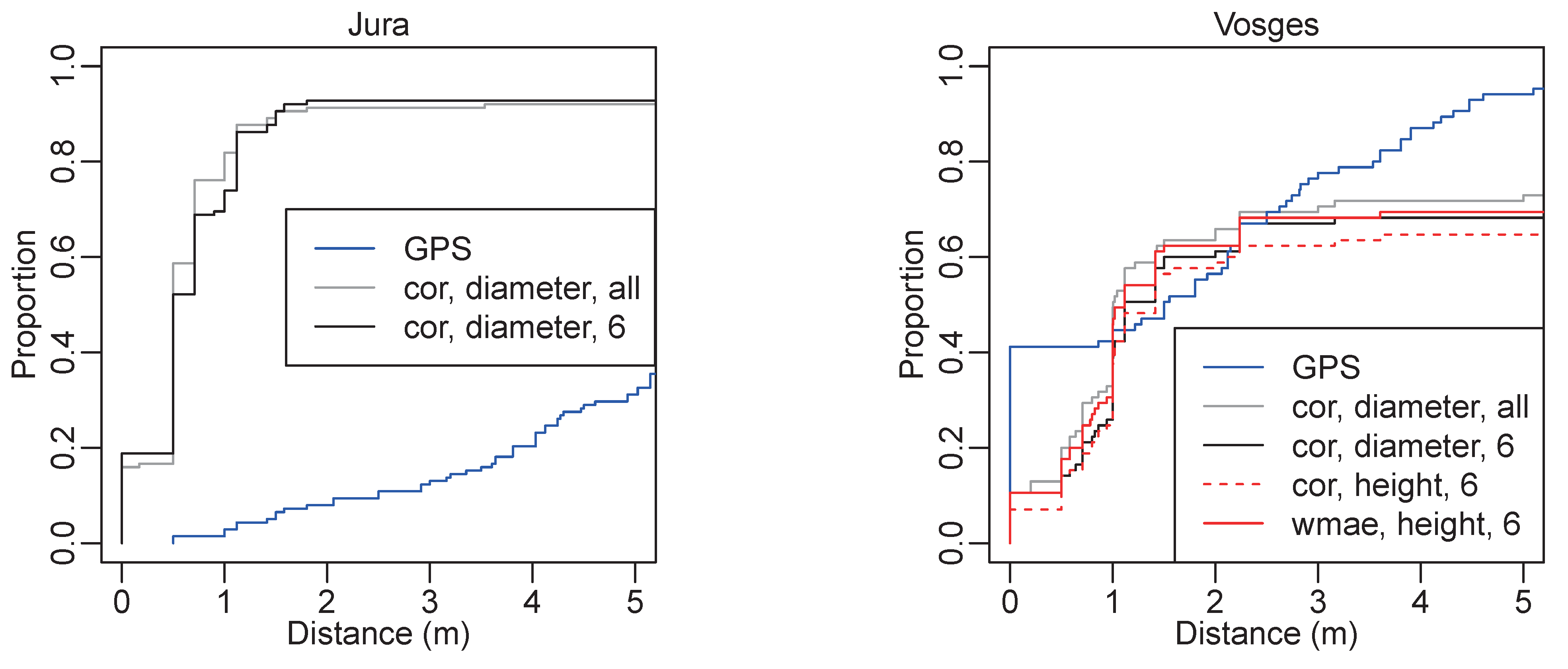
4.1.2. Algorithm Comparison

When the cor method is used with all diameters, the proportion of validated plots located no further than two meters away from the operator position is 91.3% for the Jura dataset and 65.8% for the Vosges dataset. These proportions increase respectively to 92.0% and 71.7% when the distance is below five meters. When the cor method is used with all available heights (Vosges study area), the proportions are smaller, respectively, 63.5% and 69.4% for two-and five-meter distances, but only six trees were sampled. With six diameters, the correlation results are lower, with, respectively, 61.2% and 68.2% for two-and five-meter distances. When the wmae method is used with six heights, the proportions decrease to 61.2% and 65.9%. Those results for the two-and five-meter distance thresholds are similar to the general tendency of the cumulative distribution (Figure 4). In the Vosges study area, the best co-registration is obtained with all diameters. With six values, using heights instead of diameters yields better results. The wmae method gives lower accuracy than the cor method.

4.1.3. Comparison of the GNSS, Algorithm and Operator Positions

Figure 4 also displays the cumulative proportion of distance between the GNSS and operator positions. Summary statistics are presented in Table 2. In the Jura area, the algorithm allows a better co-registration, as the GNSS curve is located below the curve of algorithm results. The mean distance decreases from 9.0 to 3.3 m. Meanwhile, the standard deviation slightly increases from 8.7 to 11.0 m. The improvement is also visible in the quartiles, as 75% of GNSS positions are more than 4.2 m away from the operator positions, whereas 75% of algorithm propositions lie within 1.1 m from the operator positions. In the Vosges area, the GNSS curve displays a plateau at 0.41 from zero to a 0.86-m distance. From a 1-to 2-m distance, the cumulative proportion is higher with the algorithm positions, but for larger distances, the GNSS proportion is higher. Indeed, the mean and standard deviation of errors are higher with the algorithm propositions than with the GNSS positions. The quartiles show that for more than half of the plots, the error is reduced, as the median error is 1.5 m for GNSS and 1.0 m for the cor method. However, for the other plots, the co-registration potentially leads to large errors.

Figure 4. Cumulative proportion of validated plots as a function of the distance in meters between the operator position and the Global Navigation Satellite System (GNSS) position or the algorithm position depending on the method used (cor correlation or wmae weighted mean absolute error), the input tree variable (diameter or height) and the number of considered trees (six or all). The curves are cropped to the distance interval 0–5 m.

Figure 4. Cumulative proportion of validated plots as a function of the distance in meters between the operator position and the Global Navigation Satellite System (GNSS) position or the algorithm position depending on the method used (cor correlation or wmae weighted mean absolute error), the input tree variable (diameter or height) and the number of considered trees (six or all). The curves are cropped to the distance interval 0–5 m.

Table 2. Statistics on the distance in meters between the GNSS and operator positions and between the operator positions and various algorithm propositions for the validated plots. On the first line is the mean ± standard deviation; on the second line are the quartiles.

		GNSS	cor, Diameter, All	cor, Diameter, 6	cor, Height, All	wmae, Height, All
Jura		9.0 ± 8.7	3.3 ± 11.0	3.1 ± 10.1
		4.2, 6.6, 10.7	0.5, 0.5, 0.71	0.5, 0.5, 1.1
Vosges		1.8 ± 2.1	5.4 ± 7.5	5.3 ± 7.0	5.4 ± 7.3	6.1 ± 7.5
		0, 1.5, 2.8	0.71, 1.0, 11.3	0.9, 1.1, 9.8	0.8, 1.1, 10.8	0.9, 1.4, 12.8

Table 2. Statistics on the distance in meters between the GNSS and operator positions and between the operator positions and various algorithm propositions for the validated plots. On the first line is the mean ± standard deviation; on the second line are the quartiles.

		GNSS	cor, Diameter, All	cor, Diameter, 6	cor, Height, All	wmae, Height, All
Jura		9.0 ± 8.7	3.3 ± 11.0	3.1 ± 10.1
		4.2, 6.6, 10.7	0.5, 0.5, 0.71	0.5, 0.5, 1.1
Vosges		1.8 ± 2.1	5.4 ± 7.5	5.3 ± 7.0	5.4 ± 7.3	6.1 ± 7.5
		0, 1.5, 2.8	0.71, 1.0, 11.3	0.9, 1.1, 9.8	0.8, 1.1, 10.8	0.9, 1.4, 12.8

4.1.4. Influence of Environmental Variables on Co-Registration Error

Table 3 displays Spearman’s correlation coefficient ρ between the co-registration error, considered to be the distance between the algorithm and operator positions of the validated plots, and the forest, topographic and ALS variables. For the Jura study area, the only significant correlations are with the ratios of the maximum value in the correlation image to the second local maximum value max₁/max₂ and to the median of its 3 × 3 neighborhood max₁/med₁. For the Vosges study area, the co-registration error is negatively correlated with basal area, mean diameter and coniferous proportion. When the wmae method is used, the error is positively correlated with stem density and negatively with the ALS vegetation point density. In all cases, the co-registration error is correlated with the ratio of the maximum value to the value of the second maximum in the cor image (in the wmae image, it corresponds to the first and second minima).

Table 3. Spearman correlation coefficient ρ between forest, topographic, airborne laser scanning (ALS) and co-registration variables and co-registration error (the distance between the operator and algorithm positions for the validated plots) for different algorithm settings. Significance levels: * p < 0.05,** p< 0.01, *** p < 0.001. CHM, canopy height model.

Variable	Vosges				Jura
	cor, Diameter, All	cor, Height, 6	wmae, Height, 6		cor, Diameter, All
Dominant height	−0.25 ∗	−0.11	−0.28 ∗
Basal area	−0.43 ∗∗∗	−0.40 ∗∗∗	−0.29 ∗∗		−0.05
Stem density	0.2	0.09	0.28 ∗∗		0.03
Mean diameter	−0.31 ∗∗	−0.22 ∗	−0.31 ∗∗		−0.04
Coniferous proportion	−0.54 ∗∗∗	−0.53 ∗∗∗	−0.31 ∗∗		−0.15
Slope	−0.16	−0.08	−0.05		0.14
Altitude	−0.12	−0.36 ∗∗∗	−0.37 ∗∗∗		0.04
Pulse density	0.08	0.11	−0.06		−0.05
Ground point density	0.18	0.17	−0.02		0.11
Vegetation point density	−0.08	−0.21	−0.29 ∗∗		−0.02
Points below 0.5 m density	0.19	0.18	−0.02		0.05
CHM pit-filling	−0.03	0.13	0.06		−0.11
CHM empty pixels	0.06	0.05	0.08		−0.04
max1/max2	−0.41 ∗∗∗	−0.42 ∗∗∗	0.41 ∗∗∗		−0.20 ∗
max1/med1	0.04	0.02	−0.04		0.24 ∗∗

Table 3. Spearman correlation coefficient ρ between forest, topographic, airborne laser scanning (ALS) and co-registration variables and co-registration error (the distance between the operator and algorithm positions for the validated plots) for different algorithm settings. Significance levels: * p < 0.05,** p< 0.01, *** p < 0.001. CHM, canopy height model.

Variable	Vosges				Jura
	cor, Diameter, All	cor, Height, 6	wmae, Height, 6		cor, Diameter, All
Dominant height	−0.25 ∗	−0.11	−0.28 ∗
Basal area	−0.43 ∗∗∗	−0.40 ∗∗∗	−0.29 ∗∗		−0.05
Stem density	0.2	0.09	0.28 ∗∗		0.03
Mean diameter	−0.31 ∗∗	−0.22 ∗	−0.31 ∗∗		−0.04
Coniferous proportion	−0.54 ∗∗∗	−0.53 ∗∗∗	−0.31 ∗∗		−0.15
Slope	−0.16	−0.08	−0.05		0.14
Altitude	−0.12	−0.36 ∗∗∗	−0.37 ∗∗∗		0.04
Pulse density	0.08	0.11	−0.06		−0.05
Ground point density	0.18	0.17	−0.02		0.11
Vegetation point density	−0.08	−0.21	−0.29 ∗∗		−0.02
Points below 0.5 m density	0.19	0.18	−0.02		0.05
CHM pit-filling	−0.03	0.13	0.06		−0.11
CHM empty pixels	0.06	0.05	0.08		−0.04
max1/max2	−0.41 ∗∗∗	−0.42 ∗∗∗	0.41 ∗∗∗		−0.20 ∗
max1/med1	0.04	0.02	−0.04		0.24 ∗∗

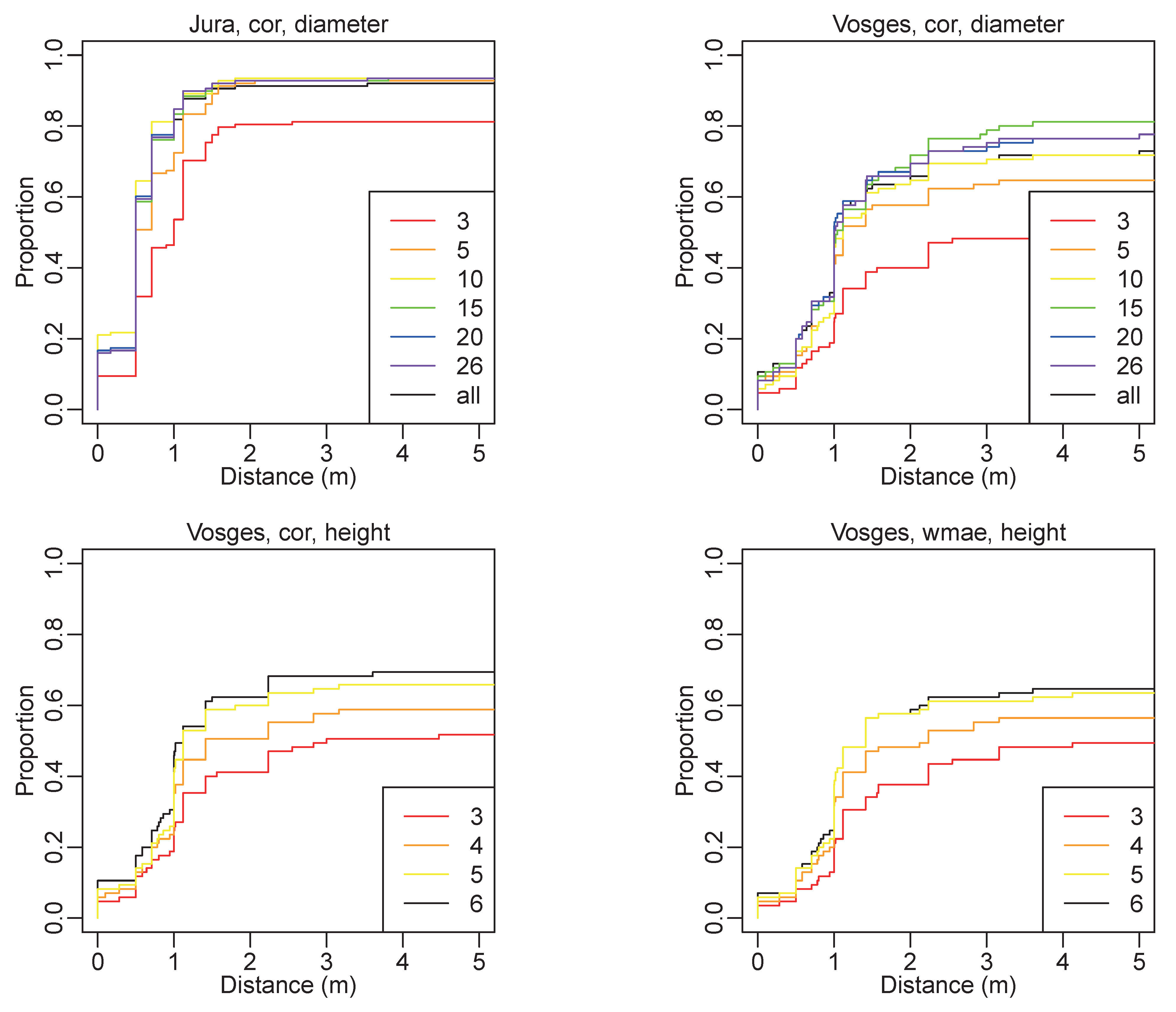
4.1.5. Influence of the Number of Sample Trees

Figure 5 displays the influence of the number of sample trees on the proportion of validated plots that are correctly co-registered. In the Jura study area, the cumulative proportion increases quickly from zero to a two-meter distance and then reaches a plateau. It is noteworthy that the proportion reached at the plateau is slightly lower when all trees are used than with a number between five and 26. The proportion of co-registration within two meters is between 91.3% and 93.5%, when more than five diameters are used. With three diameters, it is only 80.4%. The cumulative proportion of co-registered plots within one meter is also higher when only ten trees are used, compared to the proportion obtained with higher numbers of trees.

Figure 5. Cumulative proportion of validated plots as a function of the distance between the operator position and the algorithm position. Line colors refer to the sample size. Subfigure titles refer to the study area, the method used (cor correlation or wmae weighted mean absolute error) and the input tree variable (diameter or height).

Figure 5. Cumulative proportion of validated plots as a function of the distance between the operator position and the algorithm position. Line colors refer to the sample size. Subfigure titles refer to the study area, the method used (cor correlation or wmae weighted mean absolute error) and the input tree variable (diameter or height).

With the Vosges data, similar trends can be observed, except that the proportion increases more slowly and the plateau is reached around four meters. The proportion of co-registration within two meters is between 64.7% and 71.7%, when more than five diameters are used. With three (resp. five) diameters, it is only 40.0% (resp. 57.6). Whereas in the Jura area, the proportions reached at the plateau are similar when more than five trees are used, they are quite different in the Vosges area, with 64.7% for five trees, 71.7% for ten or all trees, 76.5% for 20 or 26 trees and 81.2% for 15 trees at a four-meter distance. With the Jura data, using ten trees yields a higher proportion of co-registration below one meter, but for larger distances, the proportions are similar whatever the sample size. With the Vosges data, using fifteen trees or more yields a higher proportion of co-registration, but curves then tend to diverge. In both study areas, the cumulative proportion of plots co-registered above five meters then increases slowly and more rapidly as distance increases (not shown in the figure). Indeed, in the case of a failing algorithm, which randomly chooses a position inside the investigated area, it is expected that the probability to co-register a plot at a distance d is proportional to the prospected area at this distance, which is proportional to d².

With height data in the Vosges area, trends for the cor method are similar to what is observed with diameter, but with slightly better results. The proportions of co-registered plots are 41.2% and 63.5% below two meters, 50.6% and 69.4% below four meters for three and six sampled trees, respectively. Trends for the wmae method are also similar, but with slightly poorer results. The proportions of co-registered plots are 37.6% and 61.2% below two meters, 48.2% and 65.9% below four meters for three and six sampled trees, respectively.

4.2. Prediction Models

With the Jura dataset, the selected independent variables are h_s,0.2, h_f,0.6 and CHM_>2 when the GNSS positions are used for the training data, h_f,0.8, h_mean and CHM_>2 with the algorithm positions and h_f,0.4, d_0.5 and CHM_mean with the operator positions. With the Vosges dataset, the selected variables are h_mean, d_0.83 and CHM_>2 (GNSS), h_l,0.8, d_0.83 and CHM_mean (algorithm) and h_mean, d_0.83 and CHM_>2 (operator). The mean values of the root mean square error (RMSE) of basal area prediction models obtained in 1000 ten-fold cross-validations are presented in Table 4. With the Jura dataset, the estimation of RMSE is mainly affected by the positions of the validation data. It is around 7.2 m²·ha⁻¹ with the GNSS data, 6.4 with the algorithm data and 6.0 with the operator data. With the Vosges dataset, the value of the RMSE is lower when the GNSS or operator positions are used (around 9.45) than with the algorithm positions (around 9.59), but the tendency is reversed when the algorithm positions are used for the modeling.

Table 4. Root mean square error of basal area prediction models (1000 repetitions of ten-fold cross-validations) depending on the plot positions used in the calibration and validation steps, for the two study areas. Units are in m²·ha⁻¹.

Calibration	Validation (Jura)				Validation (Vosges)
	GNSS	cor, Diameter, All	Operator		GNSS	cor, Diameter, All	Operator
GNSS	7.13	6.49	6.09		9.46	9.58	9.42
cor, Diameter, All	7.17	6.44	6.03		9.72	9.31	9.62
Operator	7.34	6.37	5.88		9.47	9.60	9.43

Table 4. Root mean square error of basal area prediction models (1000 repetitions of ten-fold cross-validations) depending on the plot positions used in the calibration and validation steps, for the two study areas. Units are in m²·ha⁻¹.

Calibration	Validation (Jura)				Validation (Vosges)
	GNSS	cor, Diameter, All	Operator		GNSS	cor, Diameter, All	Operator
GNSS	7.13	6.49	6.09		9.46	9.58	9.42
cor, Diameter, All	7.17	6.44	6.03		9.72	9.31	9.62
Operator	7.34	6.37	5.88		9.47	9.60	9.43

5. Discussion

5.1. Limitations of Reference Data

With a posteriori validation of the co-registration, a bias might exist as the operator would be tempted to consider a proposition as correct, even tough he would a priori have preferred a slightly different position. This explains the high proportion of operator positions located exactly at the GNSS positions and the low number of shifts in ]0, 1[, as the operator would rather keep the GNSS position rather than move it from a distance smaller than one pixel. The absolute precision of the manual co-registration is thus expected to be around one meter [13], while the relative position precision of a tree within a plot is around 0.5 m [16]. However, this value is based on the hypothesis that the positions of the maxima of the canopy height model are a correct indicator of the positions of stems. Broadleaved trees sometimes have multiple apices, and the highest one is not systematically located above the trunk. Coniferous trees, despite a stronger apical dominance, have not always a vertical stem. If those irregularities in tree growth result in random shifts of the apices relatively to the trunks for all trees in the plot, using a sufficient number of trees should result in an unbiased estimation of the plot center position. Meanwhile, in slope areas, normalizing the digital surface model with the digital terrain model leads to a deformation of the canopy shape and a possible virtual shift of the apices of round crowns (Figure 6), such as those of broadleaved trees. Moreover, in slope areas, trees tend to bend downslope or to develop a flag-shaped crown, so that the planimetric positions of apices are located downslope (Figure 6). In such cases, the co-registration is biased, because the crowns in the canopy height model are really or virtually shifted downslope compared to tree stems. The position error then depends on the slope, crown shape and tilt of trees. Methods that rely on the comparison of the positions of local maxima [11] avoid the deformation of tree crowns if local maxima are detected in the digital surface model, but fail to handle the case of tilted trees. Indeed, the co-registration of the CHM with the tree positions results in a co-registration of tree positions with the positions of their detected crowns. Anyway, if the final objective is to improve the analysis of remote sensing data with field plots, in our case, the modeling of stand parameters with point cloud data, then it is probably interesting to co-register the tree crowns rather than stems, as crowns are the most visible part of the trees in the remote sensing data.

Figure 6. The difference between stem position and apex position in tilted trees (a); The shift of the apex position of a round crown when correcting a slope (b, c).

Figure 6. The difference between stem position and apex position in tilted trees (a); The shift of the apex position of a round crown when correcting a slope (b, c).

5.2. GNSS Accuracy in Forests

Despite this potential error in the operator-validated ground truth, results show that the GNSS measurements made in the Jura area with a recreational-grade receiver are inaccurate. Seven plots are located further than 25 m, with a maximum of 73 m, so that it might be impossible to find those plots in the next field campaign. The mean error (9.0 m) is similar to the error of 98 manually checked plots of the Austrian National Forest Inventory (8.5 m, [13]). In contrast, the results obtained in the Vosges area with a survey-grade GNSS receiver and a long acquisition time are better. For an acquisition time of 20 min, Naesset and Jonmeister [5] reported positioning errors of 0.49 ± 0.42, 0.75 ± 0.38 and 2.5 ± 2.31 m for plots whose basal areas are below 30, between 30 and 45 and above 45 m²·ha⁻¹, respectively. In the Vosges area, the values are 2.4 ± 2.5, 1.3 ± 2.0 and 2.2 ± 1.9. Surprisingly, higher errors are recorded for small basal areas, which might be due to inaccurate co-registration by the operator for stands with small trees or with a low number of trees. Errors for large basal area values are similar, but it is noteworthy that the “doubtful” plots, with potentially large errors, are not taken into account. The Scandinavian study also reported a correlation of the positioning error with basal area, whereas in both areas of the present study, no correlation was significant with any of the forest or topographic variables. This might be due to the fact that “doubtful” plots are representatives of the extreme tendencies, but missing from the analysis, and that for small distances, the error is not properly evaluated, due to approximations by the operator.

5.3. Possibility of Co-Registration

The co-registration by the operator is generally more difficult when the contrast in the CHM is low. This is particularly the case when the dominant trees are broadleaved. The crown of broadleaved trees is also less well described by ALS data in leaf-off acquisitions. With closed canopies, the absence of small gaps also makes the co-registration more difficult. Due to the spatial resolution of the CHM, the apices of small trees are also difficult to identify. In contrary, large trees, particularly broadleaved, may have a flat crown where the apex position is doubtful, especially when the CHM is distorted because of slope correction. Some plots with few trees also turned out to be difficult to co-register properly. Those observations confirm the results of previous studies where dense plots, and, more particularly, deciduous plots, had lower co-registration accuracies [11,13]. In the end, it is important to have enough trees for a better co-registration, and it is better if those trees are separated and of different sizes, which allows the operator to take advantage of the diameter information when comparing with the CHM heights. It is also crucial that the tree crowns are well represented in the CHM. If the ALS point density is too low, it is not possible to identify crowns, especially for small trees. Those empirical findings by the operator are partially confirmed by the differences between the “doubtful” and validated plots of the Vosges study area. “Doubtful” plots have significantly lower coniferous proportion and noisier CHM. They are also located lower in altitude. This link with a topographic variable might be explained by the fact that the coniferous proportion decreases with altitude (Spearman ρ = 0.39).

In the Jura study area, most trees are coniferous, and the forest stands are uneven-aged, so that on each plot, small and large trees are present, and the canopy is not closed. Moreover, the ALS point density is high, which makes it an easy case for co-registration. The main problems with this dataset are the presence of felled trees, as the ground data is one year older than the ALS data, and the very large positioning error, which requires exploring a large window.

The proposed algorithm does not rely on individual tree detection, which is implemented for pulse densities around 5–10 pulses·m⁻² [17]. For such densities, results obtained on the Jura dataset show that co-registration performs properly. When the pulse density is lower (2–4 pulses·m⁻²), but the variations in the canopy height model are sufficient to produce a maximum in the correlation image, correct results can also be obtained, as shown with the Vosges dataset. With pulse densities below one pulse·m⁻², which can still be used for the implementation of the ALS area-based estimation method, one could expect that the modeling of the canopy is not sufficient to reflect the height variation and that the proposed approach will fail. In the absence of a field reference for the correct positions, the operator validation relied on the possibility to visually match the field trees with the CHM, so that, in the case of the Vosges dataset, some plots with a very low density had to be removed from the analysis.

The choice of a coarse resolution (one meter) for the rasters is driven by the objective to limit the amount of smoothing required to remove the noise of the CHM in the case of low pulse densities. Besides, the co-registration approach relies on correlation, which is mainly influenced by the largest variations linked to large trees and canopy gaps. Those features appear in the CHM, even at this resolution. In the case of stands with only small trees, co-registration might be improved when using finer spatial resolution if the ALS density allows it. In the Vosges area, the pulse density is a limiting factor. In the Jura area, there are no plots with only small trees. Preliminary results obtained with 0.5-m resolution yielded similar results [18]. The absence of improvement with a finer resolution might be due to the accuracy of the field tree positions.

5.4. Automated Co-Registration

Dorigo et al. [13] could automatically co-register 68% of 98 plots from the Austrian National Forest Inventory in Vorarlberg within five meters of the position previously determined by an operator. Those plots consisted in a combination of fixed-area (radius = 2.6 m) and angle count sampling. The proportion of correctly co-registered plots with the Jura data is higher (92.0%), which could be linked to several factors. First the plots are of a 17-m fixed-radius, so that more trees are inventoried inside smaller surfaces, leading to a better local fit between the stand described by the inventory and the canopy height model. As stated above, the forest stands are also particularly propitious to easy co-registration, despite a one-year gap between the ground and airborne acquisitions. In Vorarlberg, the time gap is up to 2–3 years. With the Vosges dataset, the obtained co-registration proportion is similar (72%), but the conditions are different: the time gap is smaller, plots are of a 15-m-fixed radius and the proportion of deciduous plots is higher.

With aerial images and azimuth-distances measures, Korpela et al. [7] were able to position reference points with decimeter accuracy in a stand dominated by Scots pine (Pinus sylvestris), Norway spruce and birch (Betula sp.). Their method can be applied to improve the co-registration of forest inventory plots when the azimuth and distance measures are available for a sample of trees. The obtained accuracy is better than with the methods based on ALS data, yet it might decrease in the case of stands dominated by large broadleaved trees, due to the uncertainty in the manual observations of treetops from multiple aerial images. Besides, results obtained with the fully-automated ALS-based methods can be further improved by a fast manual validation and correction of the algorithm propositions, especially if a procedure is designed to flag the uncertain cases [13]. In a boreal forest dominated by Scots pine and Norway spruce, Hauglin et al. [10] co-registered 82% (resp. 51%) of 71 plots within one (resp. 0.5) meter of the reference location, using terrestrial and low density airborne laser scanning data (0.7 pulses·m⁻²). This performance should yet be confirmed in the case of broadleaved forests. With the higher ALS density in the Jura area, 82% (resp. 59%) of plots are co-registered below one (resp. 0.5) meter with the correlation approach. In the case of existing field plots, the terrestrial laser scanning method requires additional fieldwork to perform the scans and also relies on tree detection in both the aerial and terrestrial laser data. A major advantage is that no information about tree positions are required.

The comparison of co-registration methods in the Vosges area shows that the cross-correlation yields slightly better results with heights than with diameters when the same number of tree measures are used. This could be expected, as there is some variability in the height-diameter relationship, which introduces some additional noise in the correlation between the field and ALS measures of trees. However, it is better to use all diameters than just a sample of heights. In the case that all tree positions are not available, results for the Jura dataset show that only with the five largest trees, the co-registration is almost as efficient as with all trees. For the Vosges dataset, ten trees are required to achieve similar results.

The correlation method searches for the best match between the relative variations of the CHM and those of the tree measures. The use of concentric fixed-radius plots with different DBH limits is sometimes problematic. Consider a plot covered with trees of 10 cm DBH, plus a few large trees on its western part. No trees are inventoried outside of the inner plot on the eastern part. If a canopy gap whose shape matches the area with no inventoried trees on the plot is present in the investigated area, the algorithm will erroneously match the plot to this location, because the relative variation between the eastern and western part of the plot would be apparently respected. The correlation algorithm is particularly sensitive to the presence of large gaps or stand borders, in relation to the proportion of trees inventoried in the different concentric plots with different DBH limits. This might explain why co-registration results are better with a lower number of trees. When small trees are added, they are sometimes all inventoried in the inner plot with a smaller DBH limit. Besides, small trees are likely to be suppressed trees, the values of which in the tree image will not correspond to variations in the CHM, where they are overtopped by the crown of neighboring, taller trees. To handle this issue, it is possible to model the tree crowns as Gaussian surfaces in the tree image [11], but this requires prior information about the relationship between tree size and crown shape. For a better performance, it seems important to find a trade-off between the number of considered trees and their repartition in the different concentric plots, but this optimal balance will probably depend on the forest structures (height distribution and spatial repartition of trees). In the Jura uneven-aged forests, large trees are present and spatially well distributed on all plots, so that good results are attained with only five trees and the best results with ten trees.

The weighted mean absolute error method is based on the absolute values of the CHM at the trees positions. It might also be affected by the different field sampling intensity in the different radii, even though it is not as flagrant as for the cor method. As it relies on the comparison of absolute values of height, it is probably affected by errors in the field and CHM heights, which are enhanced with broadleaved trees and in slope areas. Moreover, a shift in the positions of the tree apices relatively to the tree stems is also an issue. Unfortunately, due to the low number of sampled trees, it is not possible to investigate to what extent additional height measures could improve the co-registration.

5.5. Factors Affecting the Algorithm Co-Registration Error

In absence of high precision field data, co-registration error corresponds here to the distance to the operator proposition, which is based on visual analysis of the CHM and trees positions. In the Jura study area, the cumulative distribution of errors quickly rises and reaches a plateau at a two-meter distances, which shows that the distance is small for the correctly co-registered plots. No forest, topographic or ALS variable is correlated with the co-registration error. This could be linked with the low variability of forest stands and topography, and the high quality of the ALS data on the whole forest. The ratio of the maximum of the correlation image to the median of its neighborhood max₁/med₁ indicates if the maximum is peak-shaped or round. Peak-shaped maxima correspond to situations where the shift associated with the global maximum is precise. In the Jura area, where the conditions are easy for co-registration, the question of error, hence, comes down to whether the proposed position is accurate or not.

In the Vosges area, the correlation method is affected by basal area and coniferous proportion. As mentioned before, broadleaved trees have less apical dominance and a more rounded crown, which makes the detection of the tree tops more difficult. The negative correlation with basal area is probably driven by the fact that for young stands or stands with a small number of trees, there is not enough information for a precise co-registration. The negative correlation with the mean diameter suggests that for big trees, there might be a large shift between the apices and trunks positions. In the Vosges area, both methods have a co-registration error linked with the ratio of the global maximum value to the second maximum value max₁/max₂. This ratio can be considered as a rough indicator of the signal-to-noise ratio. When its value is close to one, there are high chances that the global maxima is only an artifact caused by the irregular shapes of trees or to a low-quality CHM.

One would expect the ALS density to be a factor affecting co-registration; however, this is not significant in any dataset. In the Vosges area, the effect of ALS density might be hidden by the variability of forests characteristics, such as basal area, coniferous proportion and, possibly, the horizontal and vertical structures, which also influence the possibility and accuracy of co-registration. In the Jura area, the pulse density is high, so that it is probably not a limiting factor in this case.

5.6. Resulting Co-Registration and Prediction Models

In the Jura area, the co-registration results in better positions compared to the initial GNSS measurements, except for a few plots that are mainly located outside of the investigated radius. In the Vosges area, there is a small improvement for approximately half of the plots, but increased error for the remaining plots.

With the Jura data, the best model is obtained with the operator positions, with an RMSE of 5.88 m²·ha⁻¹. The models obtained with the GNSS or algorithm positions and validated with the operator positions have only a slightly lower accuracy (RMSE of respectively 6.09 and 6.03). However, their “apparent” error, which is obtained when calibration and validation steps are processed with the same positions, are respectively 7.13 and 6.44. Considering that the position error results in a random noise affecting the independent variables, the result of an ordinary least squares regression will be scarcely affected by the changes in ALS variables, provided that the number of plots is sufficient and that there are no outliers. Indeed, the noise will hardly modify the coefficients of the best fit, but will increase the residuals. This might explain why the calibration step is not affected by position error, whereas it is important to have precise positions for the evaluation of the prediction accuracy.

With the Vosges data, the unsupervised co-registration leads to large errors on some plots, so that the prediction models actually have a lower accuracy than with the GNSS positions. With the low level of positioning error (mean of 1.8 m), the correction of positions does not result in significantly better prediction models, which is consistent with the results obtained at the stand level [8,9].

6. Conclusions

This study demonstrated that the cross-correlation of diameter measures is a suitable method to co-register forest plots with ALS data. Moreover, co-registration results are almost as good as with height information and are obtained with only the largest trees. The cross-correlation method displayed some limitations when used with concentric plots with different diameter inventory limits. One solution might be to automatically adapt the number of trees considered in the analysis depending on the forest structure. Moreover, one could take advantage of the sampled heights in order to compare the results of the correlation and height error methods in order to provide the operator with concordant or complementary possibilities for a faster resolution of ambiguous situations.

A comparison of the results obtained on two different datasets showed that the accuracy of co-registration and its utility for the improvement of ALS prediction models highly depends on the GNSS positioning accuracy, the ALS data quality and the forest structure. With the dataset where the co-registration performed best and where the initial GNSS precision was low, using corrected positions produces slightly better models, but mainly allows a better estimation of their accuracy. With the dataset with already accurate GNSS positions, low-density ALS data and complex, mixed forests, the unsupervised algorithm is not able to improve the co-registration. Furthermore, when the positions are improved by an operator, there are no differences in the calibration and the validation of the prediction models.

References

1. Duplat, P.; Perrotte, G. L’inventaire par échantillonnage. In Inventaire et Estimation de l’Accroissement des Peuplements Forestiers; Office National des Forêts: Paris, France, 1981; pp. 37–74. [Google Scholar]
2. Næsset, E. Predicting forest stand characteristics with airborne scanning laser using a practical two-stage procedure and field data. Remote Sens. Environ. 2002, 80, 88–99. [Google Scholar] [CrossRef]
3. Hollaus, M.; Dorigo, W.; Wagner, W.; Schadauer, K.; Höfle, B.; Maier, B. Operational wide-area stem volume estimation based on airborne laser scanning and national forest inventory data. Int. J. Remote Sens. 2009, 30, 5159–5175. [Google Scholar] [CrossRef]
4. Baltsavias, E.P. Airborne laser scanning: Basic relations and formulas. ISPRS J. Photogramm. Remote Sens. 1999, 54, 199–214. [Google Scholar] [CrossRef]
5. Naesset, E.; Jonmeister, T. Assessing point accuracy of DGPS under forest canopy before data acquisition, in the field and after postprocessing. Scand. J. For. Res. 2002, 17, 351–358. [Google Scholar] [CrossRef]
6. Andersen, H.E.; Clarkin, T.; Winterberger, K.; Strunk, J. An accuracy assessment of positions obtained using survey-and recreational-grade global positioning system receivers across a range of forest conditions within the Tanana valley of interior Alaska. West. J. Appl. For. 2009, 24, 128–136. [Google Scholar]
7. Korpela, I.; Tuomola, T.; Välimäki, E. Mapping forest plots: An efficient method combining photogrammetry and field triangulation. Silva Fennica 2007, 41, 457–169. [Google Scholar] [CrossRef]
8. Gobakken, T.; Næsset, E. Assessing effects of positioning errors and sample plot size on biophysical stand properties derived from airborne laser scanner data. Can. J. For. Res. 2009, 39, 1036–1052. [Google Scholar] [CrossRef]
9. Frazer, G.W.; Magnussen, S.; Wulder, M.A.; Niemann, K.O. Simulated impact of sample plot size and co-registration error on the accuracy and uncertainty of LiDAR-derived estimates of forest stand biomass. Remote Sens. Environ. 2011, 115, 636–649. [Google Scholar] [CrossRef]
10. Hauglin, M.; Lien, V.; Næsset, E.; Gobakken, T. Geo-referencing forest field plots by co-registration of terrestrial and airborne laser scanning data. Int. J. Remote Sens. 2014, 35, 3135–3149. [Google Scholar] [CrossRef]
11. Olofsson, K.; Lindberg, E.; Holmgren, J. A method for linking field-surveyed and aerial-detected single trees using cross correlation of position images and the optimization of weighted tree list graphs. In Proceedings of the SilviLaser 2008: 8th International Conference on LiDAR Applications in Forest Assessment and Inventory, Edinburgh, UK, 17–19 September 2008; Hill, R., Rosette, J., Suárez, J., Eds.; pp. 95–104.
12. Hyyppä, J.; Kelle, O.; Lehikoinen, M.; Inkinen, M. A segmentation-based method to retrieve stem volume estimates from 3-D tree height models produced by laser scanners. IEEE Trans. Geosci. Remote Sens. 2001, 39, 969–975. [Google Scholar] [CrossRef]
13. Dorigo, W.; Hollaus, M.; Wagner, W.; Schadauer, K. An application-oriented automated approach for co-registration of forest inventory and airborne laser scanning data. Int. J. Remote Sens. 2010, 31, 1133–1153. [Google Scholar] [CrossRef]
14. Pascual, C.; Martín-Fernández, S.; García-Montero, L.; García-Abril, A. Algorithm for improving the co-registration of LiDAR-derived digital canopy height models and field data. Agrofor. Syst. 2013, 89, 967–975. [Google Scholar]
15. Popescu, S.C.; Wynne, R.H.; Nelson, R.F. Measuring individual tree crown diameter with lidar and assessing its influence on estimating forest volume and biomass. Can. J. Remote Sens. 2003, 29, 564–577. [Google Scholar] [CrossRef]
16. Hollaus, M.; Wagner, W.; Eberhofer, C.; Karel, W. Accuracy of large-scale canopy heights derived from LiDAR data under operational constraints in a complex alpine environment. ISPRS J. Photogramm. Remote Sens. 2006, 60, 323–338. [Google Scholar] [CrossRef]
17. Vauhkonen, J.; Ene, L.; Gupta, S.; Heinzel, J.; Holmgren, J.; Pitkanen, J.; Solberg, S.; Wang, Y.; Weinacker, H.; Hauglin, K.M.; et al. Comparative testing of single-tree detection algorithms under different types of forest. Forestry 2012, 85, 27–40. [Google Scholar] [CrossRef]
18. Monnet, J.-M. Evaluation of a semi-automated approach for the co-registration of forest inventory plots and airborne laser scanning data. In Proceedings of the SilviLaser 2013, Beijing, China, 9–11 October 2013; pp. 167–174.