1. Introduction
Forestry represents a major threat to forest biodiversity by modifying and fragmenting important habitats, such as deadwood and old trees. Therefore, the preservation of biodiversity in forests is one of the major environmental challenges of our time. Spatial conservation prioritization is one of several tools to address this challenge (e.g., [
1,
2]). In this approach quantitative techniques are used to generate spatial information on which parts of the forest to prioritize for biodiversity. The early development of these methods included analysis to identify the set of reserves that maximized the total number of species included (e.g., [
3,
4,
5]). Today, in addition to a range of methodological developments, these approaches typically integrate economic and socio-political analysis into the planning process to meet the real-world prioritization challenges (e.g., [
6,
7]).
Initially, the focus of conservation planning was on nature reserves, but today, variable retention harvesting (green tree retention, GTR) [
8] is becoming the dominant biodiversity management practice in boreal forests of North-America and Europe [
9]. Retention forestry is a good example of a conservation approach that integrates biodiversity conservation with economic and socio-political realities [
10]. Another conservation measure, introduced in Fennoscandia, is woodland key habitats (WKHs) (e.g., [
11]). In contrast to the procedures in the other Fennoscandian countries, the inventory of WKHs in Norway is integrated into the forestry planning [
12,
13]. Importantly, the final selection of mapped WKHs in Norway is made through negotiations between regional forest authorities, forest owners and a biologist. Hence, the selection of WKHs in Norway is not a result of ecological values alone, but also incorporates several socio-economic values, such as cost to the forest owners. The three conservation measures can be compared as follows:
A nature reserve is typically many times larger than a forest stand, whereas a WKH is typically smaller than a stand and a retention patch a small part of a stand.
Retention patches are selected by the forest owner, the forest manager or the machine operator, whereas reserves are identified by experts. WKHs in Norway are identified by experts and selected through negotiations between experts and forest owners.
A nature reserve is typically left unmanaged, whereas WKHs and retention patches may require various silvicultural treatments to increase biodiversity.
In countries with private ownership, nature reserves usually have to be bought or compensated by e.g., the public. Retention patches, on the other hand, are required by most forest standards, and thus, they are a cost that the seller of timber has implicitly agreed upon. WKHs may sometimes be eligible for compensation (like reserves) and sometimes not (like retention patches).
This comparison implies that spatial modeling of retention patches is no different from spatial modeling of WKHs and can be treated in a similar manner. On the other hand, WKHs and retention patches should be modeled differently from nature reserves.
Although the benefits of GTR and WKHs may be varying and sometimes uncertain, WKHs are reported to be hotspots for biodiversity [
14]. For both retention patches and WKHs, a cost-benefit analysis may provide a better measure when evaluating a conservation measure. Wikberg
et al. [
15] estimated the cost of nature reserves, WKHs and GTR patches and compared the cost with the presence of large trees, deciduous trees and deadwood, as well as beetles, bryophytes and lichens. They found that reserves and WKHs have more biodiversity than retention patches, but also a higher cost.
A promising approach for improving the cost-benefit ratio of WKHs is to apply optimization techniques. Several variants of the reserve selection problem (RSP) have been formulated for nature reserves (e.g., [
16]), either as the maximization of some environmental value with budget constraints or the minimization of cost with environmental constraints. Such an approach was used by Perhans
et al. [
17], who found that cost-benefit ratios varied in six different types of retention patches. Juutinen
et al. [
18] used exact and heuristic solution methods for different RSP formulations to select stands for retention. They found that exact methods in general yielded better cost-benefit ratios and that the marginal species coverage diminished with increasing total cost.
Nature reserves typically have unmanaged forests, whereas WKHs or retention patches may benefit from various silvicultural treatments (e.g., [
19,
20,
21,
22]). There are some studies of the cost-benefit of different silvicultural treatments. Howard and Temesgen [
23] studied the estimated net profit of nine silvicultural prescriptions. Both the prescriptions and the harvesting cost calculations were on the stand level and, thus, not adapted to retention patches. Jonsson
et al. [
24] did a cost-benefit simulation of how six types of coarse woody debris (CWD) varied with seven management options. One of the management options was retention of small parts of the area, but their focus was the environmental values. Furthermore, their cost estimates were at the stand level.
The harvesting cost is a major influence on forest revenues and, hence, on the calculations of the lost forest revenues from imposing restrictions, such as retention patches (opportunity cost). A forest is typically modeled as a set of spatial units (e.g., parcels, stands or a grid), and the harvesting cost (as well as other parameters and variables) is associated with the spatial units. The harvesting cost can be divided in the work done by a harvester (felling, cross cutting and limbing) and by a forwarder (loading, unloading and terrain transportation). Of these work tasks, the terrain transportation cost is the task that is most dependent on the spatial layout and the main focus in this study. As remote sensing techniques and computational power have evolved, the size of the spatial units have decreased, and the cost calculations have changed somewhat. Traditionally, the harvesting cost has been calculated using a road density function or an average distance to the road [
25,
26], possibly using adjustments for difficult terrain or non-regular trail and road layout [
27]. When the grid size decreases, instead of calculating the cost of harvesting a spatial unit as a function of the spatial unit’s distance to the road, the cost can be calculated as a sum of costs going through neighbors (a path) to the roadside. Such an approach can be called a path calculation method. A common approach is to use a shortest path algorithm, a method used by Tan [
28], who calculated the cost as a function of distance and terrain class. Contreras and Chung [
29] used a skidding cost derived from the regression model by Han and Renzie [
30], including distance and slope gradient uphill or downhill. In a more recent paper, Contreras and Chung [
31] refined the skidding model to also include a maximum roll limit. Chung
et al. [
32] used a cost based on distance.
Data from modern remote sensing techniques are of high quality and precision, but such data may not be fully utilized in the forest industry and in forest research. Studies of the economic and environmental impacts of retention patches may benefit from more detailed data, and in particular, the path calculation method for the harvesting cost is promising [
33]. A WKH or a retention patch can be a very small part of a stand, and using a stand for the calculations may be too coarse. However, the method may be refined. Early forest machine stability studies reported that forest machines are more sensitive to roll than pitch [
34,
35], but studies of how driving speed varies with micro topography are missing in the literature [
31].
The aim of this study is to fill parts of this gap by introducing a novel way of calculating terrain transportation cost from airborne laser scanning (ALS) terrain data, including both roll and pitch estimated from micro topography. Further, the micro terrain transportation model is used in a path calculation model, yielding detailed estimates of net profit. Finally, a scenario-based multi-objective optimization model to find the opportunity cost of different silvicultural treatments of WKHs and retention patches is applied to four real-world cases. This is a method using
a posteriori articulation of preference [
36], today sometimes referred to as a generate first, choose later approach [
37]. Such approaches are suitable for solving multi-objective problems if the generated solutions can be easily assessed by a decision maker.
2. Methods and Cases
The method presented here will be described in three parts:
Section 2.1 presents the micro terrain cost model;
Section 2.2 presents the shortest path model; and
Section 2.3 presents the scenario assessment. In
Section 2.4, the cases are described.
The basic assumption is that a digital terrain model generated from ALS data is accurate enough to find the resulting roll and pitch of a forest machine driving on the terrain. Higher roll and pitch at a grid point is assumed to increase the cost of driving the machine at that particular point.
The terrain is given by a weighted graph G = (V, E), where each vertex vi ∈ V represents a point in the terrain with coordinates and elevation and has a timber volume Ui from the nearby area. The edges E link each vertex with its neighbors, and the weight of each edge is the terrain transport cost Cij = C(vi, vj).
Other assumptions are that the location of suggested hotspots for biodiversity (e.g., retention patches or WKHs) are given in advance and that the forest road network is not extended.
2.1. Micro Terrain Cost Model
As studies of how driving speed vary with micro topography are missing in the literature [
31], a simple model penalizing roll and pitch was used. The cost of transporting timber from vertex vi to a neighboring vertex
vj in uneven terrain is given by Equation (1), where
C0 is the cost of driving 1 meter (back and forth) in flat terrain and
dij is the distance from
vi to
vj.
Pr is the penalty for roll, given by Equation (2), and
Pp is the penalty for pitch, given by Equation (3).
The roll
r in Equation (2) and pitch p in Equation (3) are calculated using the difference in the elevation at some vertices in the vicinity of the wheels of a forest machine and are given by Equations (4) and (5).
rf is the roll at the front axle; and
rb is the roll at the back axle,
i.e., the percentage of inclination between the wheels on the axle.
elf ,
erf,
elb and
erb are the mean elevation at each wheel or bogie, and
df,
db and
dp are the mean distances between the coordinates of the vertices (
Figure 1). Note that on flat terrain,
r and
p are zero, and hence,
Pr = 1 and
Pp = 1. Here,
Cij =
C0dij. If the terrain is steep in the driving direction (pitch) or perpendicular to the driving direction (roll), either penalty factor will be larger than one and positive. This will increase the estimated cost of driving at that location.
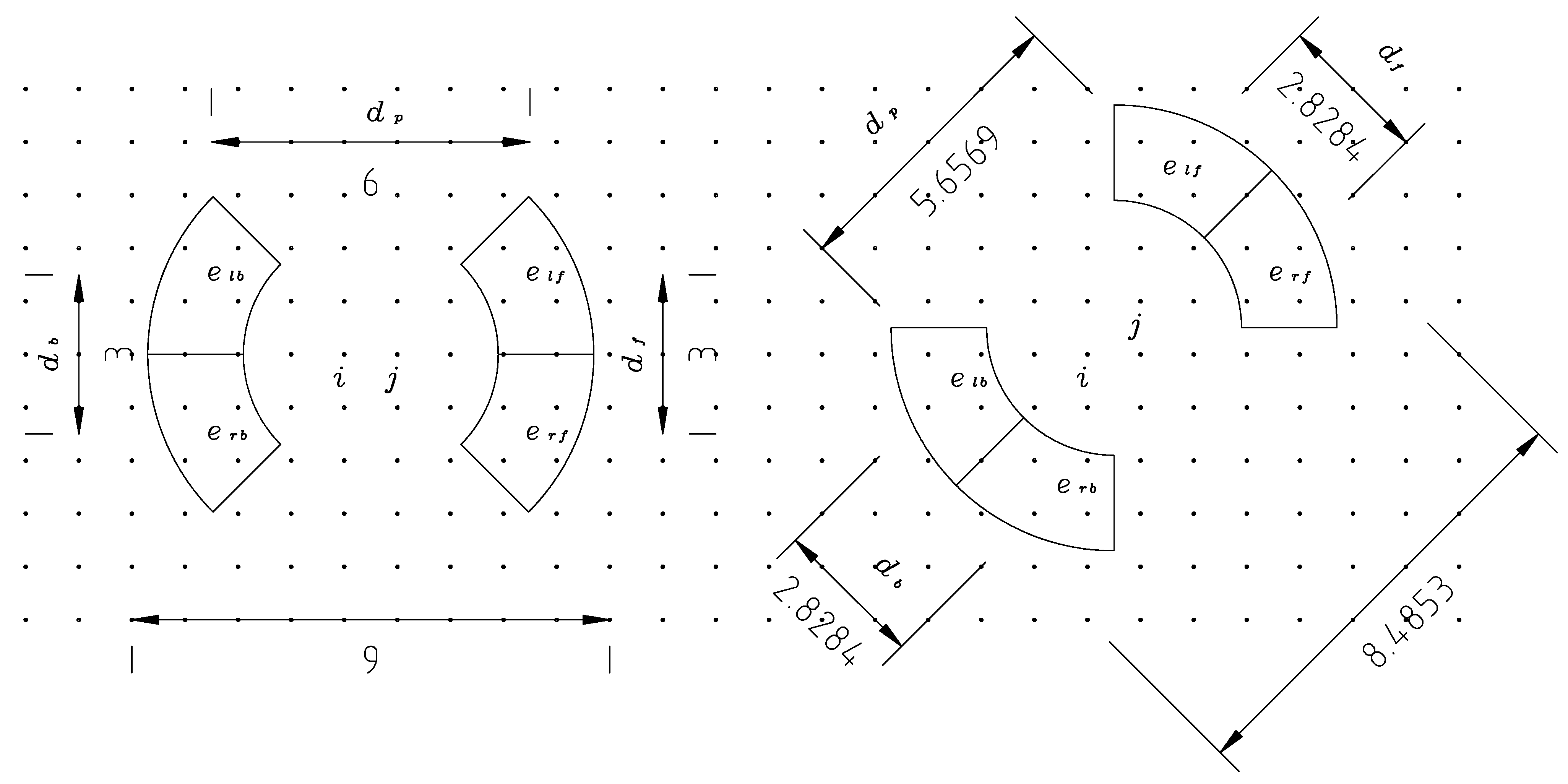
Figure 1.
Sectors used for calculating forwarding cost on a 1 m × 1 m grid (distances in meters). elf, erf, elb and erb are the mean elevation at each wheel or bogie, and df , db and dp are the mean distances between the coordinates of the vertices. The sectors are determined by a circle of radius 2.4 m, a circle of radius 4.2 m, the line in the driving direction and lines 45° left and right of the driving direction.
2.2. The Shortest Path Model
The aim of the shortest path model is to find the most efficient extraction trails from all vertices
vi to a vertex
vr that is an existing road, on a weighted graph representing the terrain. The term “shortest” may be misleading, but this problem is generally acknowledged as “the shortest path problem”. A path from vertex
v0 to vertex
vk is given by
p = (
v0,
v1,...,
vk), and the cost (weight) of transporting timber on this path is the sum of its constituent edges, given by:
where
C(
vi−1,
vi) is found by Equation (1). The shortest path cost
of using the shortest path from vertex
vi to roadside is given by minimizing:
A forest machine has a crane reach of approximately 10 m, whereas DTMs with a resolution of 1 m × 1 m are commonly used in the literature. For this reason, it may be worthwhile to define the variable forwarding cost as:
where
d(
vi,
vj) is the distance between the vertices and
d is the crane reach.
The net profit of a vertex
vi is given by Equation (9) and is the timber volume
Ui at the vertex, multiplied with timber revenue at the roadside, Π, minus harvesting costs. The harvesting cost consists of the cost of felling, cross cutting and limbing (
Ch), the cost of loading and unloading the forwarder (
Cf) and the variable forwarding cost (
Ci), the latter given by Equation (8). The term “variable” refers to the fact that
Ci is calculated as a function of transportation distance and micro terrain, described in
Section 2.1.
Finally, the net profit is the sum of net profit from all vertices with positive net profit:
2.3. Scenario Assessment
The final part of the model is the scenario assessment. Each scenario is assumed to represent a silvicultural treatment and, thus, to have varying profitability, modeled by rules for the calculation of net profit. The environmental impact of silvicultural treatments may also vary, and challenging decisions appear when the profit and the environmental values are conflicting. In this situation, the rules for calculating the profit of a scenario also include one or more rules that can be referred to as “environmental restrictions”. These environmental restrictions cause the net profit to decrease compared to a scenario with none or only some environmental restrictions. An opportunity cost of the environmental restrictions will thus be the difference in the net profit for the two scenarios.
The scenario assessment part is to compare the net profit of the scenarios and calculate the opportunity costs. If the environmental values can be assessed by an expert and there are few scenarios, the cost and benefit of each scenario can be a basis for choosing silvicultural treatments.
One advantage of this approach is that multi-objective optimization can be done without specifying a second objective function for environmental values. Non-monetary objective functions can be hard to define, and sometimes, the evaluation of non-monetary values can be easier to assess by a decision maker after the calculations.
2.4. Cases
The model was tested using four real-world cases, all located at Mathiesen Eidsvold Værk (MEV) (latitude 60.44, longitude 11.07), a large forest property in Norway (
Table 1). The cases were selected in collaboration with a forest manager, and the main criteria were that the terrain should be suitable for the harvester-forwarder system and that WKHs should be somewhat close to a forest road. Each case had one or more WKHs, but retention patches were not included. This choice was made to keep the cases simple and easier to analyze. Furthermore, WKHs and retention patches would be treated in the same way in the model.
Table 1.
Cases.
| Case | Total area (ha) | WKH area (ha) | WKH area (%) |
|---|
| 1 | 111 | 13.6 | 12.2 |
| 2 | 94 | 6.5 | 6.9 |
| 3 | 203 | 18.8 | 9.3 |
| 4 | 345 | 24.2 | 7.0 |
Within each case, five scenarios were used, based on the manual for WKHs in Norway [
38,
39,
40]. In Scenario 1, vertices
vi inside the WKHs were not harvested (
Ui = 0) and driving was not allowed (
C(
vi,
vj) = ∞). For Scenarios 2–5, driving in WKHs was allowed, but the harvest was limited to 0%, 30%, 70% and 100%, respectively. The scenario with 100% harvested volume is, in fact, the same as ignoring the WKH area completely.
The results by Nurminen
et al. [
41] were used to find an estimate of
C0. Their observed maximum speeds while driving loaded and unloaded were assumed to be in the flattest terrain, and the average of the two was 73 m min
−1. A forwarder hourly cost of $175 h
−1, a forwarder load capacity of 14 m
3 and a delay factor of 1.33 give
C0 = $7.57 × 10
−3 m
−3 m
−1.
The maximum roll limit was set to
rmax = 0.23, and the maximum pitch limit was set to
pmax = 0.35 in the calculations, as a conservative estimate based on static stability studies [
34,
35].
The average timber price used was Π = $50 m
−3. The other parameters of the model were calculated from an hourly harvester cost of $200 h
−1, an hourly forwarder cost of $175 h
−1 and average values of Nurminen
et al. [
41] and were found to be
Ch = $7.4 m
−3 and
Cf = $5.0 m
−3.
The terrain was represented by a raster grid with a resolution of 1 m × 1 m, generated from a high accuracy ALS dataset. Each grid point was linked with the eight neighbors, and the timber volume at each grid point was Ui = 2.37 × 10⁻² m3. (i.e., 237 m3 per hectare).
The shortest path costs (
) given by Equation (7) were found using Dijkstra’s shortest path algorithm [
42]. As the resolution was high, Equation (8) was used to find the variable forwarding costs.
3. Results and Discussion
The calculated net profit for each scenario and case is given in
Table 2. As the calculated net profits are due to the selected cost model, it seems appropriate to start this section by discussing the cost model and subsequently going into detail about how the scenarios can be used for assessing the impact of retention patches.
Table 2.
Objective values for scenarios and cases. WKH, woodland key habitat.
Table 2.
Objective values for scenarios and cases. WKH, woodland key habitat.
| Scenario | Description (WKH treatments) | Case 1 ($) | Case 2 ($) | Case 3 ($) | Case 4 ($) |
|---|
| 1 | No trails, no harvest | 637,339 | 700,233 | 1,360,604 | 2,286,526 |
| 2 | Trails, no harvest | 662,430 | 700,438 | 1,360,642 | 2,288,134 |
| 3 | Trails, 30% harvest | 686,301 | 712,867 | 1,404,178 | 2,340,318 |
| 4 | Trails, 70% harvest | 718,129 | 729,440 | 1,462,227 | 2,409,897 |
| 5 | Trails, 100% harvest | 742,001 | 741,869 | 1,505,763 | 2,462,082 |
3.1. Cost Model
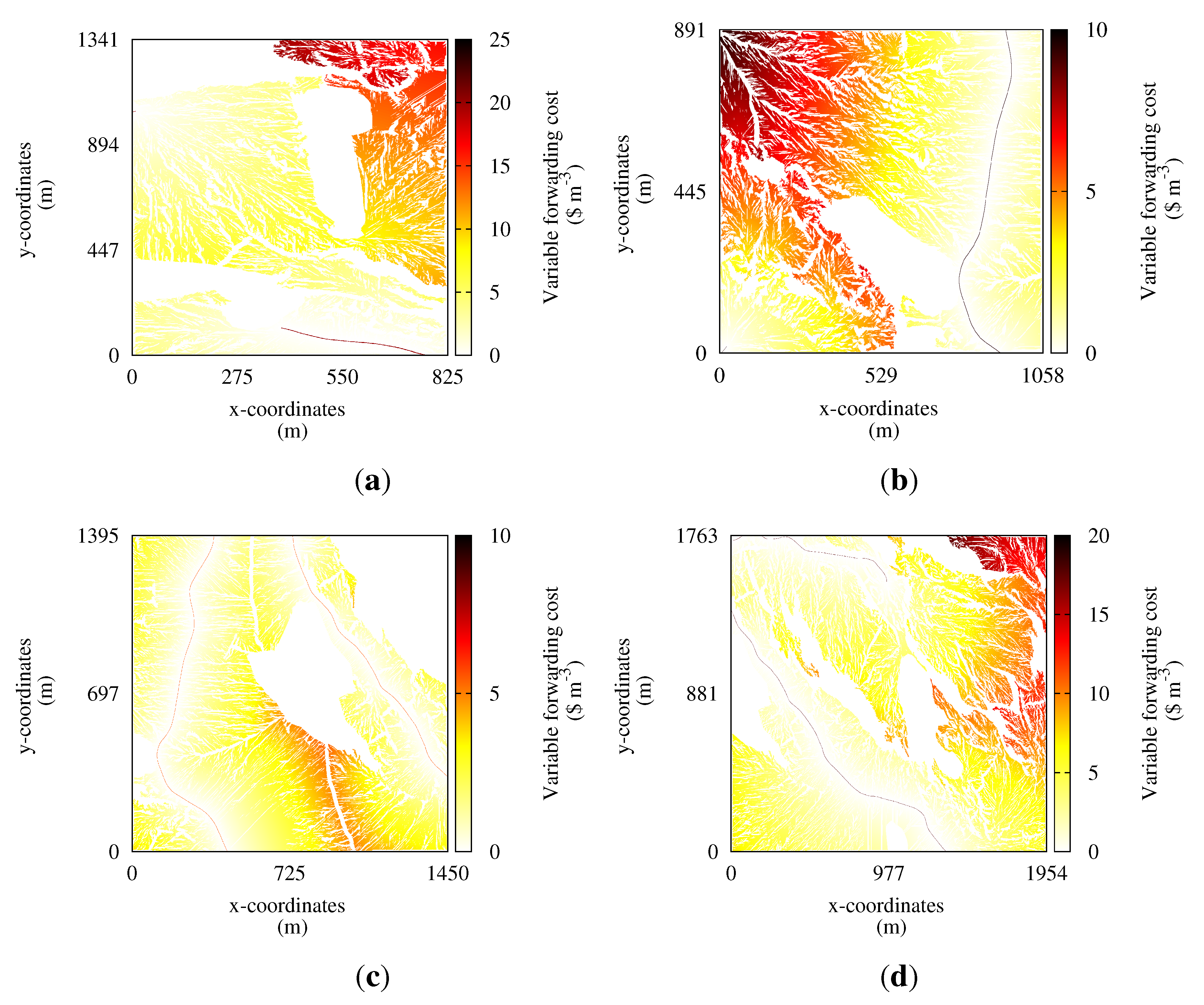
The shortest path optimization returned the variable cost of forwarding, and the maximum cost was found in Case 1, Scenario 1, at $20 m
−3 . A heat map of the variable forwarding cost for Scenario 1 for all cases is given in
Figure 2. A visual inspection reveals that the variable terrain transportation costs are in general increasing with the distance to the road, as would be expected from traditional cost calculations. However, in all cases, there are areas where the costs are significantly higher than in areas nearby, indicating difficult terrain or that the micro topography is causing detours.
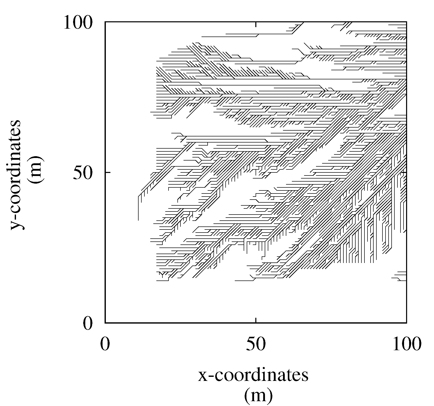
In the cost model, logs at a vertex are assumed picked up and transported to the roadside through the shortest path.
Figure 3 shows that the shortest path model gives a dense path network. In reality, only some of the trails will be used when the area is harvested, as a forwarder (and the harvester) would use trails, collecting what is reachable from the trails. However, the estimated forwarding cost will be quite good, because the cost of transportation in parallel trails is almost equal, otherwise there would be more merging of trails. In fact, the variable forwarding cost estimate will be a lower bound compared to a less dense solution, giving a sound estimate of the cost.
On the other hand, trails with a transit volume of more than a minimum volume can easily be found, and such main extraction trails are likely to be used by a forwarder. A forwarder operator will collect timber until the machine is fully loaded and then use the shortest paths to the roadside (
i.e., the main extraction trails). The main extraction trails for Case 1, with more than 40 m
3 transit volumes, are shown in
Figure 4.
Figure 2.
Heat maps of the variable forwarding cost. Roads can be seen as dotted, dark red curves. (a) Case 1. Note the short forest road ending close to x = 0, y = 1000; (b) Case 2; (c) Case 3; (d) Case 4.
Figure 2.
Heat maps of the variable forwarding cost. Roads can be seen as dotted, dark red curves. (a) Case 1. Note the short forest road ending close to x = 0, y = 1000; (b) Case 2; (c) Case 3; (d) Case 4.
Figure 3.
Part of the solution of Case 1, showing the density of the trails. Note that the calculated forwarding costs of parallel trails are almost equal, and a real forwarding operation would not use all of the plotted trails.
Figure 3.
Part of the solution of Case 1, showing the density of the trails. Note that the calculated forwarding costs of parallel trails are almost equal, and a real forwarding operation would not use all of the plotted trails.
Figure 4.
Main extraction trails for Case 1 (transit volumes > 40 m3). The red curves are forest roads. Note the short forest road ending close to x = 0, y = 1000. (a) Driving in WKHs not allowed, no harvest in WKHs (Scenario 1); (b) driving in WKHs allowed, no harvest in WKHs (Scenario 2). The main extraction trails inside the WKHs are for transportation of timber harvested outside the WKH. The main extraction trails appear to start inside the WKHs, but this is due to merging of trails with transit volume less than 40 m3.
Another simplification of the model is the cost of felling, cross cutting and limbing,
Ch, as well as the fixed cost of forwarding,
Cf. In the model, these costs are independent of the harvest percentage inside the WKHs. In general, both
Ch and
Cf will increase when the harvested volumes per area decrease (e.g., [
41]). Although a tabular correction of these costs, as a function of volume per area, can be implemented without affecting the computational complexity much, a more detailed formulation of the loading phase was suggested by Flisberg
et al. [
43]. By describing the phase as a vehicle routing problem (VRP), they found significant improvements. However, the VRP is known to be NP-hard and, thus, not suitable for the model presented here.
The estimated variable forwarding costs rely on the quality of the digital terrain model (DTM) and the choice of micro topography cost model. ALS is commonly used for forest inventory surveys, in some countries systematically (e.g., Sweden and Finland). However, factors such as dense vegetation or steep terrain, reduce the quality of DTMs (e.g., [
44]) and may require higher point density than default. Another option for improving the quality of DTMs is to use the full-waveformat (e.g., [
45]). As noted by Contreras and Chung [
31], no productivity studies with this level of detail are presented in the literature. In fact, forwarding productivity studies are reported for forwarding cycles and not adapted to shortest path models at all. It is an open research question whether productivity functions will vary with the resolution of digital terrain models.
In the presented model, a cost of terrain transportation in flat terrain of
C0 = $7.57 × 10
−3 m
−3 m
−1. The maximum possible penalty is
Pr ·
Pp = 1.97, and hence, the maximum possible terrain transportation cost is
Cij = $1.49 × 10
−2 m
−3 m
−1. Contreras and Chung [
29] used a variable skidding cost of $2.03 × 10
−2 m
−4 (flat and downhill) and $2.44 × 10
−2 m
−4 (uphill). Chung
et al. [
32] used a variable skidding cost of $5 × 10
−2 m
−4, but also $2.5 × 10
−2 m
−4–$1 × 10
−1 m
−4 in the sensitivity analysis. This may indicate that either the value used for
C0 or the penalty factors are too low or that forwarding is cheaper than skidding. Hopefully, future productivity studies, including micro topography, will verify the model used or supply better models.
3.1.1. Model Sensitivity
Any change in the parameters of the model will change the net profit, but not necessarily the shortest path solution. The maximum terrain transportation cost in all of the cases was found to be $20 m−3 (in Case 1, Scenario 1), resulting in a minimum marginal profit of $17.6 m−3. As Equation (10) requires that only economically viable timber is harvested, the price of timber can decrease by $17.6 m−3 without changing the shortest paths. Likewise, the cost of felling, cross cutting and limbing and the fixed cost of forwarding could each increase by the same amount without changing the shortest paths. Furthermore, if the marginal net profit decreases below $0 m−3 at a vertex vi, the shortest paths would remain unchanged up to that vertex. The model’s sensitivity to C0 is similar, but the penalty factors make it difficult to predict the limits of C0 where changes in the paths occur.
To evaluate the model’s sensitivity to the limits for roll and pitch in the penalty factors, the net profits were calculated for different maximum values of roll between 0.21 and 0.33 and different values of maximum pitch between 0.33 and 0.43 for Case 1, Scenarios 1–2. The relative values obtained are given in
Table 3. The ratio of net profit of Scenario 1 to net profit of Scenario 2 seems to be stable. However, the indirect opportunity cost is decreasing as maximum roll and/or maximum pitch increase, and a roll limit of 0.29 and a pitch limit of 0.39 give a ratio that is higher than 99%.
Table 3.
Net profit for Scenario 1 divided by net profit of Scenario 2 for different roll and pitch limits (Case 1). Ratios close to one mean that there are small differences between the net profit of Scenario 1 and Scenario 2 (i.e., low indirect opportunity cost).
Table 3.
Net profit for Scenario 1 divided by net profit of Scenario 2 for different roll and pitch limits (Case 1). Ratios close to one mean that there are small differences between the net profit of Scenario 1 and Scenario 2 (i.e., low indirect opportunity cost).
| Max pitch | Max roll |
|---|
| 0.21 | 0.23 | 0.25 | 0.27 | 0.29 | 0.31 | 0.33 |
|---|
| 0.33 | 0.968 | 0.972 | 0.959 | 0.959 | 0.985 | 0.985 | 0.984 |
| 0.35 | 0.958 | 0.962 | 0.959 | 0.986 | 0.987 | 0.988 | 0.988 |
| 0.37 | 0.958 | 0.983 | 0.983 | 0.987 | 0.987 | 0.992 | 0.992 |
| 0.39 | 0.964 | 0.984 | 0.986 | 0.988 | 0.993 | 0.994 | 0.995 |
| 0.41 | 0.985 | 0.989 | 0.988 | 0.992 | 0.995 | 0.996 | 0.997 |
| 0.43 | 0.988 | 0.992 | 0.995 | 0.996 | 0.996 | 0.996 | 0.997 |
For Cases 2–4, there were few differences between Scenario 1 and Scenario 2 (
Table 4), and the calculated ratios for varying maximum roll and pitch were all close to 1.0.
Table 4.
Opportunity costs.
Table 4.
Opportunity costs.
| Opportunity cost | Case 1 | Case 2 | Case 3 | Case 4 |
|---|
| WKH area, A (ha) | 13.6 | 6.5 | 18.8 | 24.2 |
| Reachable WKH area, A* (ha) | 10.5 | 5.0 | 17.7 | 22.7 |
| Total opportunity cost,
OCT ($) | 104,662 | 41,636 | 145,159 | 175,556 |
| Average total opportunity cost, OCT ($ha−1) | 9,989 | 8,325 | 8,218 | 7,724 |
| Direct opportunity cost,
OCD ($) | 79,571 | 41,431 | 145,121 | 173,948 |
| Average direct opportunity cost, OCD ($ha−1) | 7,594 | 8,284 | 8,215 | 7,653 |
| Indirect opportunity cost,
OCI ($) | 25,091 | 204 | 38 | 1,608 |
| Average indirect opportunity cost, OCD ($ha−1) | 2,395 | 41 | 2 | 71 |
3.2. Scenario Assessment
The scenarios have different environmental restrictions. By comparing the net profit of different scenarios, the opportunity costs of the environmental restrictions can be found. In
Table 4, the total opportunity cost,
OCT, is the difference in the objective value of Scenario 5 and Scenario 1. The direct opportunity cost is the part of the total opportunity cost that can be located to areas inside the retention patch. This is calculated as the difference in the net profit of Scenario 5 and Scenario 2. The indirect opportunity cost is the part of the total opportunity cost that can be located to areas outside of the retention patch and is calculated as the difference in the net profit of Scenario 2 and Scenario 1. The average opportunity costs are the opportunity costs divided by the reachable WKH area.
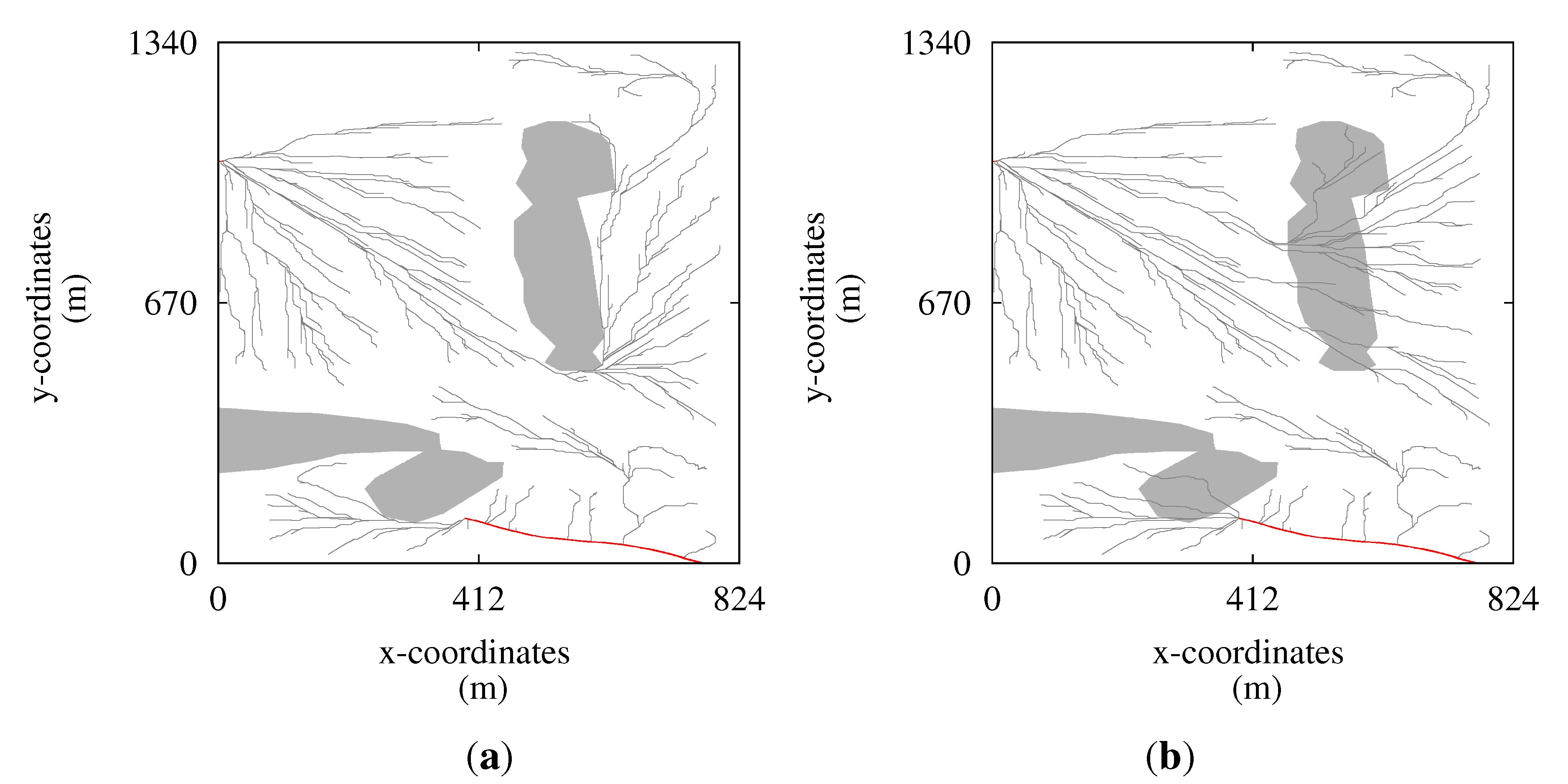
The indirect opportunity cost was found to be negligible in Cases 2–4, but $25.091 in Case 1. This increase in net profit was partly due to a 0.6 ha increase in harvested area, i.e., the area that was not reachable without driving through the WKHs. This resulted in an increase in harvested volume of 147 m
3 . The average net profit per volume for Case 1, Scenario 2, was $32.3 m
−3, and the average value of the increased harvested volume is thus $4.746. The rest of the increased net profit is due to reduced terrain transportation cost found at 31 ha (
Figure 5).
Figure 5.
Woodland key habitats (dark gray) and areas with reduced terrain transportation cost from driving through the WKH area (light gray), Case 1.
Figure 5.
Woodland key habitats (dark gray) and areas with reduced terrain transportation cost from driving through the WKH area (light gray), Case 1.
The problem of selecting silvicultural treatments for WKHs is assumed to consist of the net profit as one objective and also an objective of environmental values, which is not calculated explicitly. Even with this simplification, the number of possible outcomes is large, and a generic discussion is needed. The silvicultural treatments have impacts both on the net profit and the environmental values, and a treatment should be chosen by evaluating tradeoffs in the objectives. This evaluation may occur at different stages of the process.
An environmental value may dictate preservation of the area. Such a decision is usually made by a political body, and the cost of compensation may be a part of the decision. At this stage, the cost-benefit analysis must be done by the political body.
A political body may impose guidelines or rules for the forest management or there may be negotiations between a forest standard agency and the forest owners.
A forest manager may choose within the rules or guidelines.
The presented method can be a useful tool for all of the listed stages. An example of use at Stage 3 can be Case 1 in
Table 4, where the indirect opportunity cost is large. A large indirect opportunity cost means that not being allowed to drive in the WKHs is expensive, A single extraction trail through the WKH of this case would reduce the cost of harvesting, but leave most of the WKH unharmed. If there were guidelines allowing trails through the WKHs, a forest manager would choose that option.
Another example could be to assume that harvesting is planned for the four cases, and the guidelines require that a minimum area is not harvested. With this assumption, a forest manager would first preserve the WKHs in Case 4, as this has the lowest average opportunity cost, and then continue with the WKH area with the second lowest opportunity cost. Note that the choice in this case would depend on the guidelines for driving through the WKHs in Case 1; in fact, if driving were allowed there, Case 1 would be chosen first, as Case 1 has the lowest average direct opportunity cost.
The method can also be used by the public when designing the guidelines for the forest managers (Stages 1 and 2). A scenario-based presentation is easy to understand and shows a trade-off between environmental impact and net profit. This can be useful when considering which policy to implement or when compensation may be given. Such a presentation may also be an asset if the forest manager can negotiate with the public what silvicultural treatments to implement.
3.3. Model Evaluation and Some Limitations
When building an optimization model, the model will be a simplification of the real world, and the input data will have measurement errors. In addition, some model formulations are intractable for computers [
46],
i.e., at some problem size, the time or memory needed to find the optimal solution exceeds physical limits. One such class of problems is the class of NP-hard optimization problems, which have no known exact solution method for large problem instances. Large problem instances can either be formulated as a simplified model and solved to optimality, or they can be optimized using non-exact methods (e.g., heuristics or metaheuristics). In the latter case, the solutions found may not be optimal ones. The presented model is a two-step model, where the first step solves using Dijkstra’s shortest path algorithm and the second step compares different scenarios. This is a simplified model that can be solved to optimality very fast, a crucial feature when optimizing large problem instances. The computational complexity of Dijkstras’ shortest path algorithm is
![Forests 05 02327 i002]()
(
n log(
n)) [
47],
i.e., the time needed to find the solution is bounded by a constant multiplied by
n log(
n), where
n is the problem size.
The computer times were around 25 min for the largest case (Case 4). The shortest path model was solved using C++ from the GNU Compiler Collection, and Linux (on a Dell Optiplex 990 with Intel® CoreTM i7-2600 processors).
The opportunity costs found by the method are given in
Table 4. The results are in the same range as in the literature, but a direct comparison is difficult, because net present value is frequently used. Wikberg
et al. [
15] found that WKHs had an opportunity cost of €5.277 ha
−1 and that retention patches were significantly cheaper. The latter was also found by Perhans
et al. [
17]. Jonsson
et al. [
24] simulated different silvicultural treatments in southern, middle and northern Sweden, and the opportunity cost of setting aside stands as reserves in middle Sweden was SEK43.424 ha
−1, which is of the same magnitude as the opportunity cost given by Wikberg
et al. [
15] and the results presented here (
Table 4).
As the micro topography cost model is independent of the shortest path model, the scenario-based method can easily be adjusted for other wheel-and ground-based extraction systems, e.g., skidders, farm tractors or horses. Cable yarding systems, on the other hand, have not been modeled as a shortest path problem in the literature, but rather as a facility location problem (e.g., [
48]). Scenario-based optimization of opportunity costs could still be implemented, but the shortest path part would have to be replaced with a cableway facility location routine. Planning extensions of the forest road network also usually lead to facility location formulations. Facility location problems are generally NP-hard, and including such aspects in the model would not be straightforward.
3.4. Implications for RSP
The scenario-based optimization model can be utilized to generate input for the RSP for WKHs or retention patches (GTR-RSP). A GTR-RSP formulation requires some environmental value in the objective function or in the constraints, and this will vary according to the silvicultural treatments in the scenarios. The corresponding opportunity cost can be found in
Table 4. In the test cases, a uniform timber volume of 237 m
3 ha
−1 was used, and it was also assumed that all of the areas were mature forest. In reality, different stands in the forest would be of different age and have varying timber volume. The net present value of a future opportunity cost (or profit) can be easily found, but the time aspect and stands were not implemented in the cases.
The presented generate first, choose later approach is applicable as long as the number of possible treatments and the resulting environmental values are easily assessed by a decision maker. These assumptions will in general not be met for a GTR-RSP formulation. Selecting different treatments for a large number of WKHs and retention patches while assessing numerous environmental values is not an easy task. Formulating and solving a GTR-RSP will require high quality input data. Some of the costs could be estimated as presented in this work, and
4. Conclusions
The presented model can be utilized for detailed calculations of the cost of forest operations, thus getting better estimates of the cost of the conservation of retention patches. This can, in turn, be utilized for conservation prioritization. This work has shown that both the variable forwarding cost and the opportunity cost of retention patches vary significantly given the input data and assumptions. However, these assumptions should be studied further, in particular how the driving speed is affected by the micro topography.
We introduced a separation of the opportunity cost into direct and indirect opportunity cost and found that in three of four cases, the indirect opportunity cost was negligible. In one of the cases, it was shown that the retention of a WKH may affect the cost of forest operations in surrounding areas.
The model should be applied to an RSP case for retention patches. This would require it to be adapted to the environmental values and silvicultural options found in the specific RSP case.


 (n log(n)) [47], i.e., the time needed to find the solution is bounded by a constant multiplied by n log(n), where n is the problem size.