Article

Estimating Near-Surface Soil Hydraulic Properties through Sensor-Based Soil Infiltrability Measurements and Inverse Modeling

1
School of Technology, Beijing Forestry University, Beijing 100083, China
2
College of Information and Electrical Engineering, China Agricultural University, Beijing 100083, China
*
Authors to whom correspondence should be addressed.
Forests 2024, 15(3), 569; https://doi.org/10.3390/f15030569
Submission received: 15 January 2024 / Revised: 18 March 2024 / Accepted: 19 March 2024 / Published: 21 March 2024
(This article belongs to the Section Forest Soil)

Abstract

:
Near-surface soil hydraulic properties (SHPs) are fundamental for describing and predicting water and energy exchange processes, particularly at the soil–atmosphere interface, and regulating evapotranspiration, infiltration, and runoff in different ecosystems. In this study, a new method was proposed to estimate near-surface SHPs by combining sensor-based soil infiltrability measurements with inverse modeling using HYDRUS-2D. The infiltration rate (IR) was estimated by combining the linear source inflow method with image processing, and Ks was estimated from the near-surface steady-state IR (NSIRM). The SWRC parameters described by the van Genuchten model were estimated using the inverse modeling method of HYDRUS-2D for the fitting of sensor-measured infiltration data. Subsequently, the parameters of the van Genuchten model, including α , n , and l , were inversely estimated. Three undisturbed soils, including two stand humus samples from cork oak (Quercus suber L.) and oleander (Pinus tabuliformis L.) stands and one sandy loam from a farmland, were sampled near the soil surface to validate the proposed method. The estimated Ks was evaluated by the constant head method (CHM). The estimated parameters of the SWRC were validated by those determined through the simultaneous measurement of the soil moisture content and water potential using sensor techniques. The results showed that the Ks estimated from the NSIRM for each soil sample were 23.40 ± 1.21, 23.86 ± 1.83, and 22.99 ± 2.26 mm h−1, respectively. In comparison, the Ks determined by the CHM were 24.41 ± 1.53, 24.26 ± 0.37, and 23.81 ± 0.10 mm/h, respectively. The relative errors of the proposed method were 4.14%, 1.64%, and 3.42%, respectively. For the SWRC estimation, the normalized root mean square errors (NRMSEs) between the measurements and the estimates for each soil sample were 0.1724, 0.1454, and 0.0606, respectively. Based on this, the AWC was obtained, and Ku was deduced from the estimated Ks and SWRC parameters for each soil sample. In general, the proposed method successfully estimates near-surface SHPs, simplifies the measurement device, and provides a new perspective for the in situ determination of near-surface SHPs under field conditions in the near future.

1. Introduction

Knowledge of soil hydraulic properties (SHPs) is essential to assess the water cycle in ecosystems [1]. This includes knowledge regarding the infiltration rate (IR), soil water retention curve (SWRC), available water capacity (AWC), and hydraulic conductivity (K), which are all important parameters for determining the quality of the soil environment and the capability of the soil to serve the ecosystem. In contrast to other land uses, studies reveal that forest soils usually show higher hydraulic conductivity [1,2,3]. Moreover, the infiltration capacity and soil water retention in forested soils control the formation of surface runoff, acting as a natural flood regulator [3,4]. Compared to deeper soil layers, the SHPs near the soil surface are subject to rapid changes in response to changes in soil properties, interactions with water (rainfall, infiltration, evaporation), and biopores created by the decomposition of the root. Thus, near-surface SHPs are fundamental for describing and predicting water and energy exchange processes, particularly at the soil–atmosphere interface, regulating evapotranspiration, infiltration, and runoff.
In recent years, studies have witnessed remarkable progress in determining the saturated hydraulic conductivity (Ks), unsaturated hydraulic conductivity (Ku), soil water retention curve (SWRC), and available water capacity (AWC) of SHPs; however, the infiltration rate (IR) has rarely been investigated. In other words, it is difficult to obtain all SHPs from a single method based on existing studies.
Diverse commercial sensors, devices, and methods have been developed and applied under both laboratory and field conditions to determine Ku directly or indirectly. For instance, previous studies have applied a method to determine Ku by measuring soil water potential (ψ) at two soil depths using the Buckingham–Darcy equation during an evaporation process [5,6,7,8,9]. However, this method requires the simultaneous application of multiple sensors, which not only increases the cost, but also decreases the measurement accuracy, owing to sensor-to-sensor uncertainties [10,11]. Consequently, the indirect method has been applied to determine Ku using the measured Ks [12,13,14,15,16,17], and the fitted parameters of SWRC based on hydraulic models [14,18].
Ks can be determined using a single-ring permeameter [19], a Guelph permeameter [20], or a dual-ring permeameter in the field, whereas the falling method or the CHM is employed in the laboratory [21,22,23,24]. The SWRC can be measured using the ceramic pressure plate extractor [25]. However, due to the difference in contact area between the soil and the plate, the measurements of the pressure plate lack reliability in the dry range [26]. Other existing methods for SWRC estimation include fractal geometry, pedo-transfer functions (PTFs) [27], soil morphology, and empirical models.
Mathematical modeling plays a crucial role in estimating SHPs, thus providing valuable insights into water movement in the subsurface. Various methods and tools have been developed to capture the complex relationships between soil properties and hydraulic behavior. Here, we delve into different approaches employed in mathematical modeling for hydraulic property estimation. Numerical simulation models, such as finite element or finite difference methods, allow for a more detailed representation of the soil profile, like HYDRUS, SWAP, and MODFLOW. Numerical models demand computational resources and data-intensive input, making them challenging for certain applications [28]. Pedo-transfer functions (PTFs) are empirical equations that estimate SHPs based on easily measurable soil characteristics. These functions leverage statistical relationships derived from extensive soil databases. PTFs provide a quick and practical way to estimate SHPs, but may have limitations in capturing site-specific variations like soils under conservation or conventional agriculture [29,30]. Recent advances in machine learning (ML) have introduced innovative techniques for estimating hydraulic properties. ML algorithms, including support vector machines, neural networks, and random forests, can learn complex patterns from large datasets. These data-driven approaches offer flexibility and adaptability to diverse soil conditions. But ML approaches may be considered “black-box” models, making it challenging to interpret their internal workings.
In fact, most studies have only measured Ks, Ku, and SWRC, and only a few have measured the IR and AWC. AWC is defined as the ability of soil to store water between the field capacity (FC) and the permanent wilting point (PWP). FC refers to the amount of water retained in the soil after any excess water has drained out, leaving the soil saturated but not waterlogged. It represents the maximum amount of water the soil can hold against the force of gravity and is available for plant use. PWP is the soil moisture content at which plants are unable to extract more water, leading to irreversible wilting. It is the lower limit of plant-available water in the soil, indicating the point at which the soil water potential becomes too low for plants to sustain normal growth [31,32]. Veihmeyer and Hendrickson [33] used sensor measurements, in situ moisture content monitoring, and the laboratory measurements of soil cores in pressure chambers to directly acquire the AWC. It is worth mentioning that the FC is an empirical concept whose physical definition remains under discussion [34]. Th FC is generally defined as the soil moisture content (θ) retained at ψ levels approximately between −10 and −33 kPa, whereas the PWP represents the SWRC at −1500 kPa [35]. Hence, the FC and PWP are defined as the θ at the −33 kPa and −1500 kPa, respectively, based on the estimated SWRC in this study. The above-mentioned parameters are associated, except for the IR, which can be estimated using the linear source method [36] and point source method [37].
This study proposes a new method that uses a simplified device for estimating near-surface SHPs. Assuming soil samples are homogeneous, a steady flow rate is provided to the soil during the experimental process. The soil wetting area is collected via the use of image sensors, while the soil moisture information is obtained using moisture sensors. Both multi-sensor measurements and inverse modeling methods were used to estimate the IR, Ks, SWRC, Ku, and AWC. The SHPs estimated by the proposed method are validated against those estimated by traditional methods. Upon ensuring the accuracy of this method, it is demonstrated that only two sets of data, namely the wetting area and soil moisture information, combined with an inversion module, are required to obtain SHPs.

2. Materials and Methods

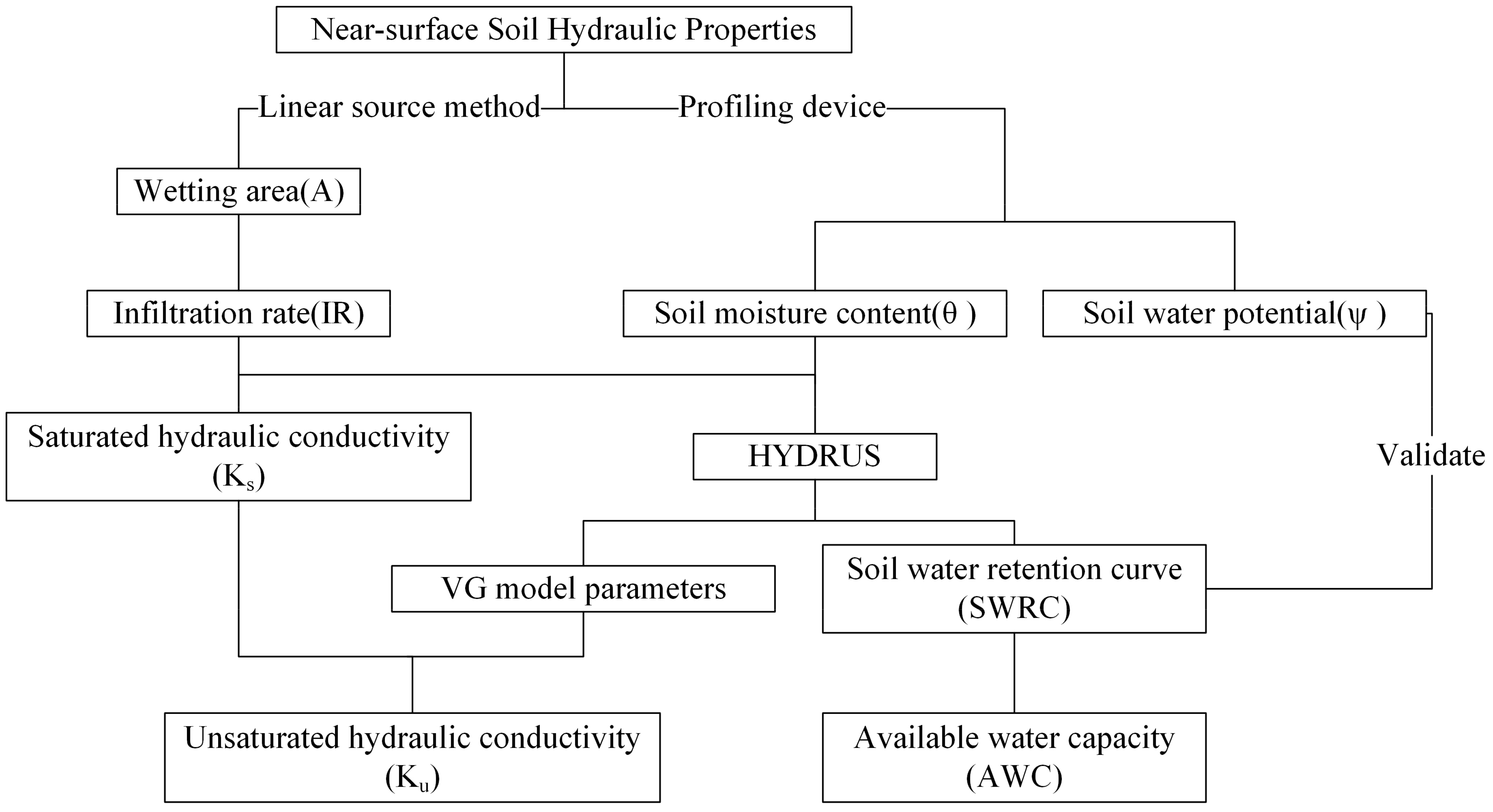
2.1. Mathematical Models for the Estimation of the Near-Surface Soil Hydraulic Properties

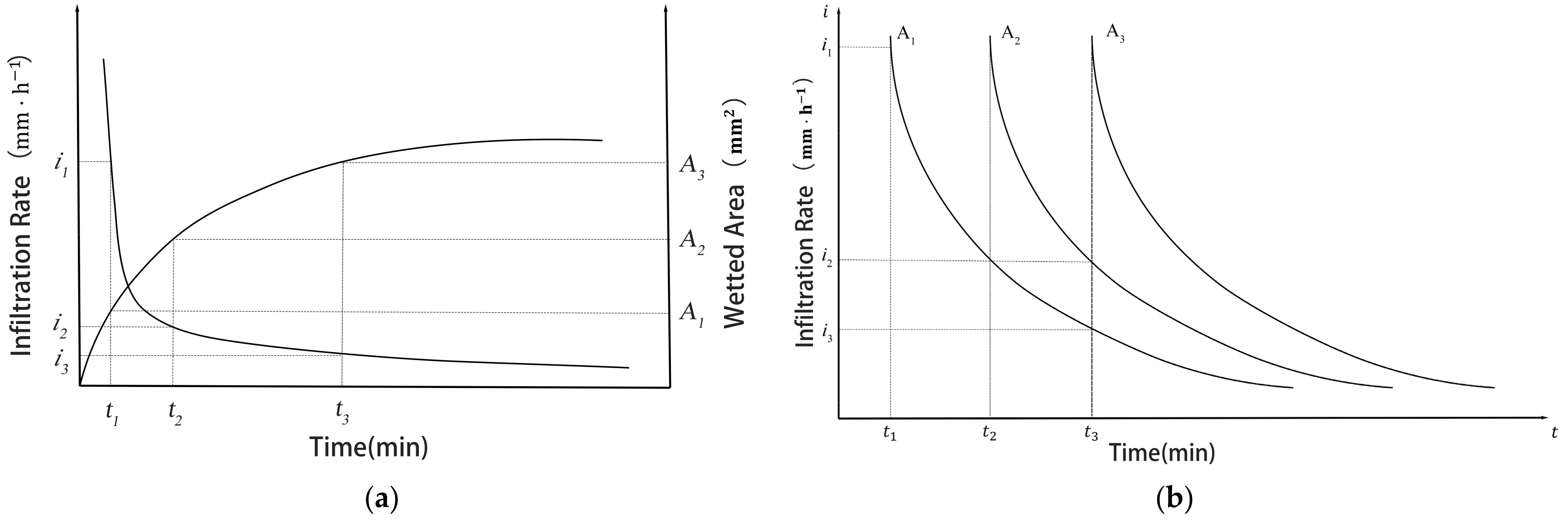
2.1.1. Linear Source Inflow Method for Estimating Soil Infiltration Rate and Saturated Soil Hydraulic Conductivity

Assuming the soil is uniform and non-layered, when the soil moisture content near the soil surface saturates during the water infiltration process, the soil IR approaches a constant value (steady-state IR), which is commonly considered to be the Ks value. To determine the soil IR, a linear source inflow method proposed by Mao et al. [36] was combined with the camera image processing method to estimate Ks. Assuming a near-uniform soil texture and a sufficient water supply, the soil water infiltration process can be calculated using the relationship between the soil-wetted area and time (Figure 1a). Initially, the wetting area is near zero, but has the highest IR. Subsequently, the IR and the increase in the wetting area gradually decrease. When the wetted area and the IR reached the steady-state value, Ks was estimated from the steady-state IR.
However, during the process of surface water flow, the starting time of the IR at different points on the surface is different. Figure 1b illustrates the distribution of the IR at different spatial locations and times. At time t1, the water has just reached spatial point A1, where the soil IR is the maximum initial value, denoted as i1. Subsequently, at time t2, the water has just reached the spatial point A2, where the IR remains at the initial value of i1. However, at this time, the IR performance at the spatial point A1 has decreased, as indicated by the curve in Figure 1b, which has decreased to i2. As time progresses to t3, the IR at points A1 and A2 have decreased to i3 and i2, respectively, following the trend shown in Figure 1b.
The relationship among the soil IR, the wetted area in the horizontal direction, and the time during the infiltration process can be obtained using the following equation [36]:
q = 0 A i A , t d A
where q is the in-flow rate ( μ L   h 1 ) ,   i is the infiltration rate ( m m h 1 ), and A is the wetted area in the horizontal direction ( m m 2 ). In fact, directly obtaining the analytical solution of Equation (1) is challenging. Therefore, we divide time into infinitesimally small intervals, and then select the corresponding soil wetting area increment steps (∆A) for each interval. Within each time interval and ∆A, we consider the IR as the average value for that segment. At time t2 (Figure 1b), with a wetting area increment of ΔA2, the infiltration rate is i1, consistent with that observed on ΔA1 at time t1. However, the IR on ΔA1 decreases to i2 at this moment. Similar situations occur in other time intervals. Eventually, we iteratively derive an approximate estimate of in. The specific computational process is described as follows:
According to the principle of water flow balance at time t 1 [36],
q 1 = i 1 A 1
at time t 2 ,
q 2 = i 2 A 1 + i 1 A 2
at time t n ,
q n = i n A 1 + i n 1 A 2 + + i 2 A n 1 + i 1 A n
From Equations (2)–(4), the i n at different times is given by the following equation:
i n = q n j = 1 n 1 i j A n j + 1 A 1 n = 1,2 , 3
Finally, Ks was estimated from the steady-state i n .

2.1.2. Inverse Estimation of the Soil Water Retention Curve Using HYDRUS-2D
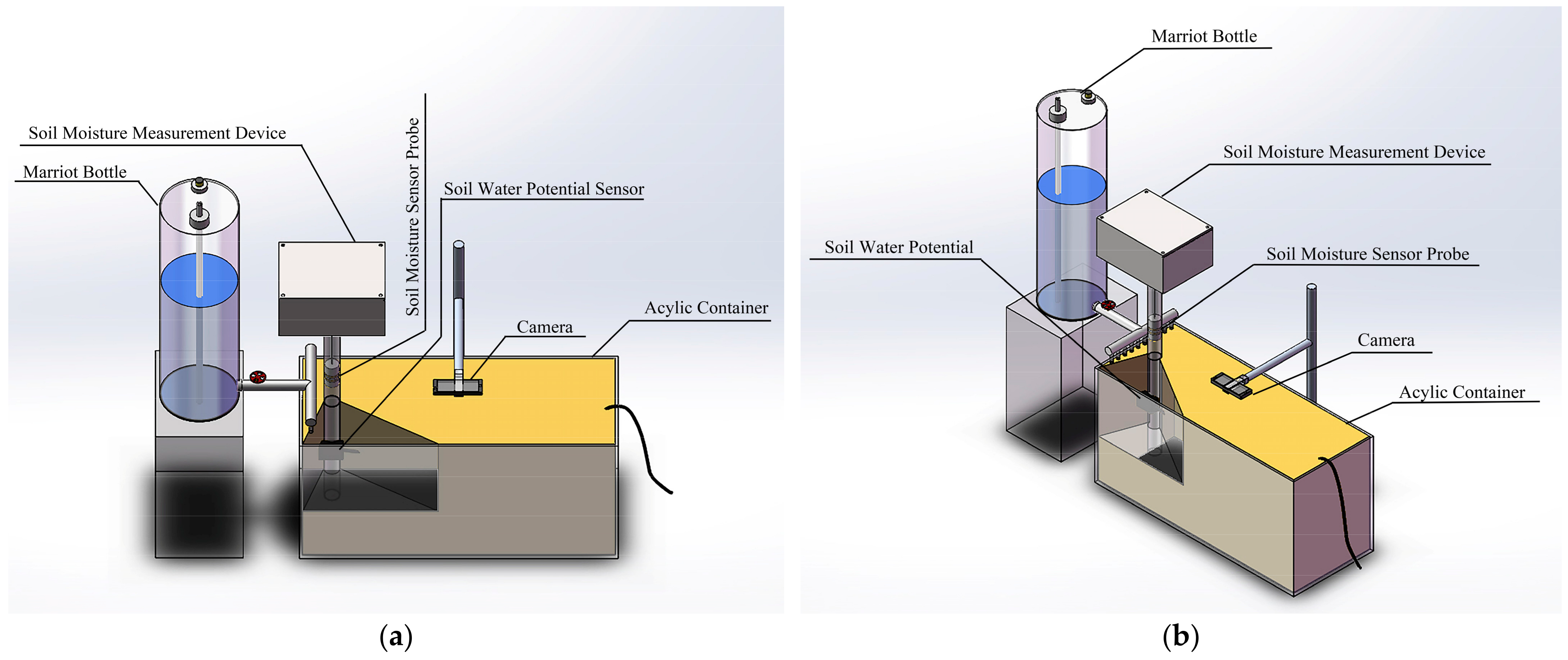
A two-dimensional soil hydrodynamic model was used to describe the soil water vertical infiltration and horizontal diffusion processes. Assuming that the soil properties and texture are identical near the soil surface and that the influence of the roots can be ignored without vegetation cover, the model can be described by Richards’ equation:
θ t = x K u ψ x + z K u ψ z + K u z
where θ is the soil moisture content ( m 3   m 3 ) , t is the infiltration time m i n ,   ψ is the soil matric potential ( k P a ), x and z are the horizontal and vertical diffusion (infiltration) distances ( m ), respectively, and K u is the unsaturated soil hydraulic conductivity.
The relationship between θ , ψ , and K u in Richards’ equation are given by the van Genuchten [10] (VG) model:
θ ψ = θ r + θ s θ r 1 + α h n m                     h < 0 θ s                                                         h 0
K u = K s S e l [ 1 1 S e 1 / m m ] 2
S e = θ θ r θ s θ r = 1 1 + α h n m
where θ r and θ s denote the residual and saturated moisture content ( m 3 m 3 ), respectively, S e is the effective saturation, α ( m 1 ) is the inverse of the air-entry value (or bubbling pressure) relating to pore-size distribution, l is a pore-connectivity parameter assumed to be 0.5 as an average for many soils [13], and m = 1 n 1 [14].
To estimate the SWRC, the inversion module of HYDRUS-2D was utilized, with the Levenberg–Marquardt (LM) algorithm being selected to optimize the parameters during the inversion process. The optimization principle of the LM algorithm is to minimize the difference between the measured and simulated variables (e.g., ψ and θ). The sum of the squares of these differences is represented by the objective function Φ , which is expressed as
Φ θ , α , n = i = 1 N θ * t i θ t i , α , n 2
where α and n are the empirical parameters of the VG model, θ * is the measured value of the moisture content of the soil vertical profile m 3   m 3 , θ is the soil moisture content when the parameter α , and n takes different values ( m 3   m 3 ) .

2.2. System Design

The system design (Figure 2) included the water supply part (Mariotte bottle, linear source water distribution device), soil moisture measurement device, image recording part (camera), a rectangular acrylic container, and a laptop. This camera model is SD-200 (Shenzhen Micro Technology Co., Ltd., Shenzhen, China), with an effective resolution of 1920 H*1080 V (2 megapixels). The outlet of the Mariotte bottle was connected to a linear-source water distribution device in order to supply water at a constant rate. The linear source water distribution device uses a copper adjustable diverter valve, placed directly above the soil surface to ensure that water linearly flows into the soil. The soil sample was filled into an acrylic container (1 m × 0.3 m × 0.2 m). The water supply rates were 27.33 ± 6.17 mL min−1, 31.33 ± 11.67 mL min−1, and 33.833 ± 8.0 mL min−1 for the soil from the cork oak (Quercus suber L.) stand, the soil from the oleander (Pinus tabuliformis L.) stand, and the sandy loam from a farmland, respectively. Commercial soil water potential sensors Teros 21 (METER Group, Inc., Pullman, WA, USA) were used to validate the estimated SWRC.
Based on the study conducted by Yu et al. [38], we designed the moisture sensor, and the diagram and photograph are shown in Figure 3. To calibrate the sensor, we used three types of soil samples which were required for the experiment: the humous soil from both the cork oak and oleander stands, and the sandy loam from the farmland. All soil samples were dried at 105 °C for 48 h, and then moistened with different water contents. Under laboratory conditions at room temperature (25 ± 1 °C), the mixed soil samples were filled into cylindrical PVC containers. The sensor surrounded by the soil samples was placed at the center of the PVC container. Table 1 displays the calibration results of the moisture sensor in the three soil samples, with the fitted correlation R2 between the sensor output and the soil moisture content ranging from 0.9887 to 0.9986.

2.3. Experimental Preparation and Procedure

2.3.1. Experimental Materials

The experimental materials used were undisturbed soil samples that were collected from two forest stands and a farmland. The humus soil samples were obtained from the surface high-organic-matter soil in the cork oak stand area and the oleander stand area of the Jiufeng National Stand Park (39°54′ N, 116°28′ E), Haidian District, Beijing, with initial moisture contents of 1.42%, and 22.93%, respectively. The sandy loam sample was taken from the 0–10 cm soil layer of San Qingyuan (40°0′ N, 116°20′ E) from the Beijing Forestry University, with an initial moisture content of 2.83%. The soil colors were determined according to the Munsell chart, with the cork oak stand soil being 5GY6/1, the oleander stand soil being 7.5Y8/4, and the sandy loam being 10Y7/2. The experiments for each sample were repeated three times. The physical properties of the soil samples are listed in Table 2.

2.3.2. Experimental Procedure

In the measurement system, a hole was drilled in the undisturbed soil samples for the in situ installation of the PVC pipe. At the beginning of the measurement, the sensor probe was controlled to descend to different depths, measuring the soil moisture content and time.
Using the linear source inflow process, images of water diffusion at the soil surface at different times were captured using a camera. Image processing technology was employed to calculate the wetting areas (A) from the pictures using OpenCV. It includes three steps: distortion correction, binarization, and counting the number of pixels. Distortion correction refers to the phenomenon in which the actual and ideal images differ because of the lens itself. The captured images were cropped to obtain the mesh corner point information to calculate the camera correction coefficient. Binarization was used to set the gray values of the pixels to 0 or 255 for each image. After binarizing the images, the number of pixels in the mesh image was determined using OpenCV. Finally, the wetting area was calculated according to the number of mesh pixels and individual mesh areas.
The inversion module of the HYDRUS-2D model was used to estimate the SWRC. In managing the experiment in 2D, we considered both the vertical (z) and horizontal (x) directions. Despite the horizontal wetting area extending in both the x and y directions, we opted for the linear source infiltration method and assumed homogeneity within the soil samples. Hence, for simplicity, we focused solely on the x direction. Consequently, in HYDRUS, we constructed a soil model with dimensions of 30 cm in the x direction and 20 cm in the z direction, divided into 1200 triangular grids. Furthermore, the inversion module was selected to simulate the water flow dynamics of the model within 120 min, with the estimated results (i.e., output data) set as the soil hydraulic parameters. The soil moisture content was used as the initial condition for the model, with initial moisture contents of the two humus soils and the sandy loam being 0.015 cm3 cm−3, 0.24 cm3 cm−3, and 0.17 cm3 cm−3. Observation points were selected at depths ranging from 2 to 5 cm, with a depth interval of 1 cm, and the soil moisture sensor was used to measure the soil moisture changes at four depth points, providing input data. Additionally, the saturation moisture content (θs) in the soil hydraulic parameters was measured from the sensor in saturated soil conditions, while the volumetric moisture content (θr) was estimated from the soil moisture characteristic curve corresponding to −1500 kPa. The Ks was obtained using the NSIRM. The remaining soil hydraulic parameters, α and n, were the output data. The upper boundaries of the three soil samples were set at flow rates of 1.64 L h−1, 1.85 L h−1, and 2.06 L h−1, respectively, to simulate atmospheric rainfall boundaries, while the lower boundary was set as a free drainage boundary.
The AWC was estimated using the SWRC. The FC and PWP of the three soils were taken from the moisture contents corresponding to −33 kPa and −1500 kPa in the SWRC, respectively. The Ku value can be calculated using the above parameters with Equation (8). A flowchart for estimating the near-surface SHPs is shown in Figure 4.

2.4. Method for Validation and Error Analysis

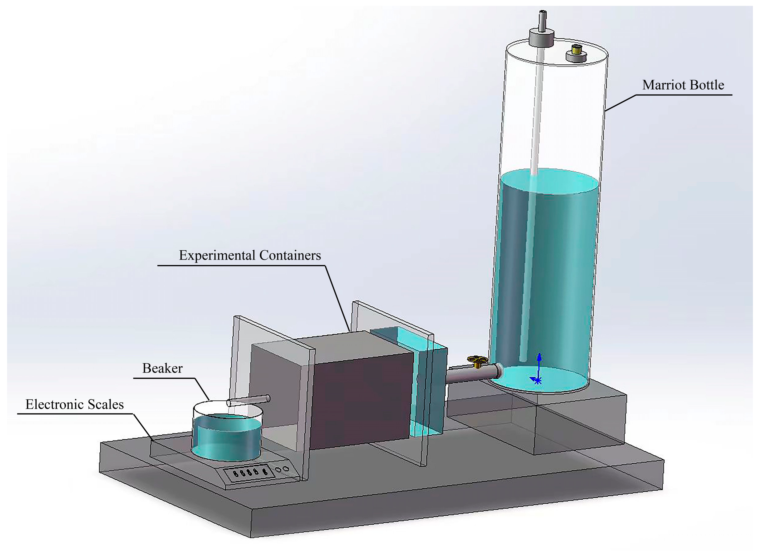
2.4.1. Validation of the Saturated Hydraulic Conductivity Using the CHM

The measurement error of Ks, estimated by the NSIRM (Figure 5), assuming the constant head measurement as the true value, can be calculated as follows:
K s = Q L A Δ h
where Q is the amount of water flowing out of the test container ( m m 3   h 1 ), L is the length of the soil column in the measurement section ( m m ), A c is the cross-sectional area of the soil column in the test container ( m m 2 ), and Δ h is the height difference between the lowest point of the conduit in the Mariotte bottle and the water outlet of the test container ( m m ). The measurement error can be calculated using Equation (12).
δ = I 2 I 1 I 2 × 100 %
where I 2 is the Ks measured using the CHM, and I 1 is the Ks value measured using the NSIRM.

2.4.2. Comparison of the SWRC and the Measured Results

The HYDRUS-2D software (v2.04) simulation was quantitatively validated using the normalized root mean square error (NRMSE) as follows:
RMSE = i = 1 N P i O i 2 N
NRMSE = RMSE O m a x O m i n
where N is the total number of observation points of θ or ψ, P i and O i are the simulated and measured values of stand θ or ψ of the ith observation point, respectively, and O m a x and O m i n are the measured maximum and minimum values of θ or ψ at the observation point, respectively. The root mean square difference represents the fitting degree between the simulated and actual values. NRMSE is the normalized RMSE, used to facilitate comparisons.

3. Results

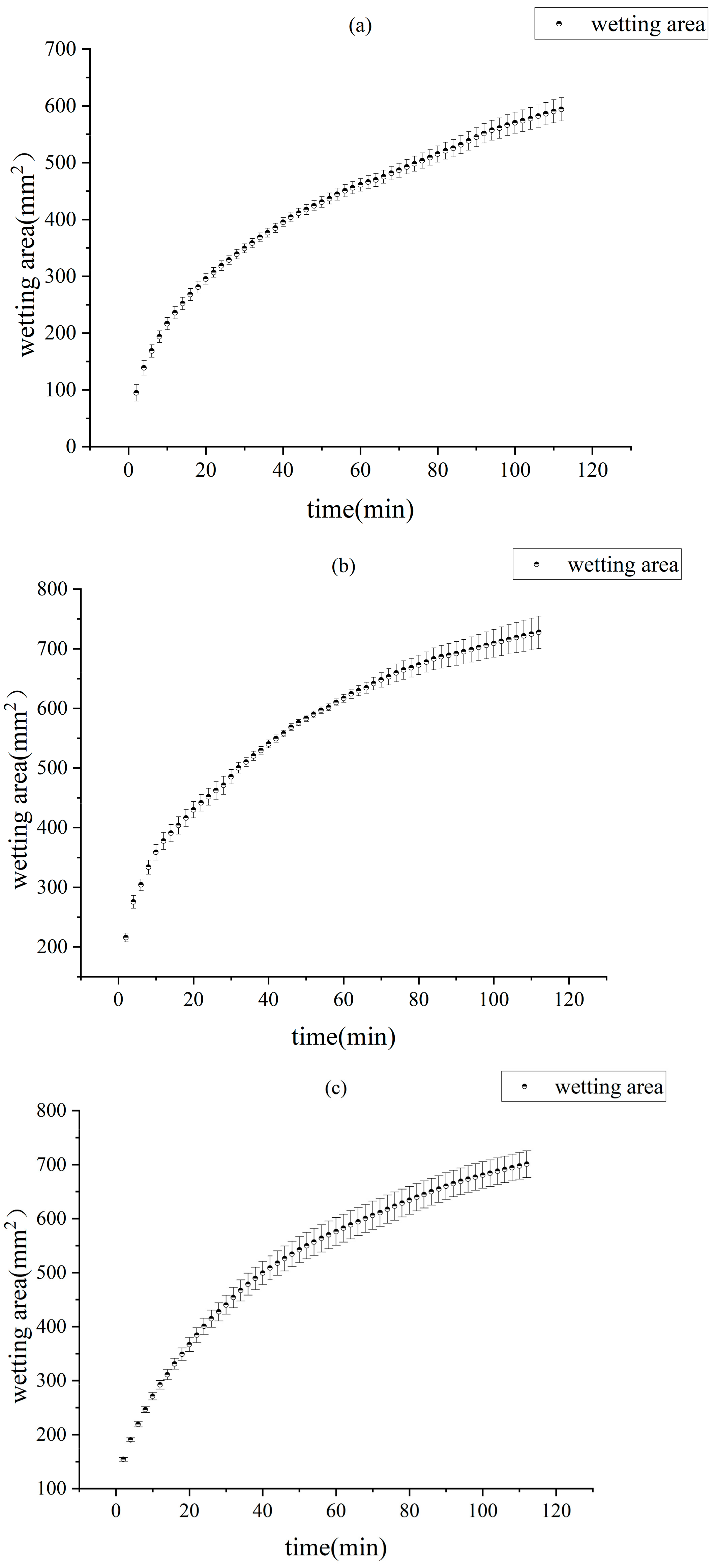
3.1. Estimation Results of the Soil Wetting Area Using Image Processing

After the experiment begins, the camera captures images of the soil wetting situation every 2 min. Here, we have chosen one example to explain the image processing process. Figure 6 shows the image processing results. A checkerboard (Figure 6a) was used to calibrate and correct the camera images, and 54 corners were extracted in order to establish the corner point coordinates (Figure 6b). According to the relationship between the corner point, world, and image coordinates, the internal and external parameter matrices and distortion coefficients of the camera were obtained, and the calibration result (Figure 6c) of the camera was 0.0766. The area of one checkerboard is 4.84 cm2 with 3600 pixels; thus, one pixel corresponds to an area of 0.134 mm2. The internal and external parameters of the camera and the distortion coefficient are shown in Figure 6d, and the corrected results are shown in Figure 6e. Following binarization (Figure 6f), the soil wetting area was calculated according to the correspondence between the pixels and the area.
We recorded the soil wetting area calculated from image processing every 2 min, and fitted it into a curve representing the change over time (Figure 7). In the initial stage, as infiltration begins, the soil wetting area gradually expands as water penetrates the soil and spreads outward. At the onset of the infiltration experiment, the rate at which the increase in the spread of the wetting area is rapid, especially when there are no significant obstacles on the soil surface. As time progresses, the rate of increase in the wetting area starts to decline because the soil has begun to saturate, and any further infiltration of water is limited or slows down. After a period of time, when the infiltration experiment ceases, the soil wetting area reaches a stable state.
The regression equations of the three soil samples according to the relationship between the wetting area and time are shown in Table 3. The coefficients of determination (R2) are 0.9938, 0.9947, and 0.9988, respectively, indicating that the regression equations can better describe the water diffusion of the soil surface over time.

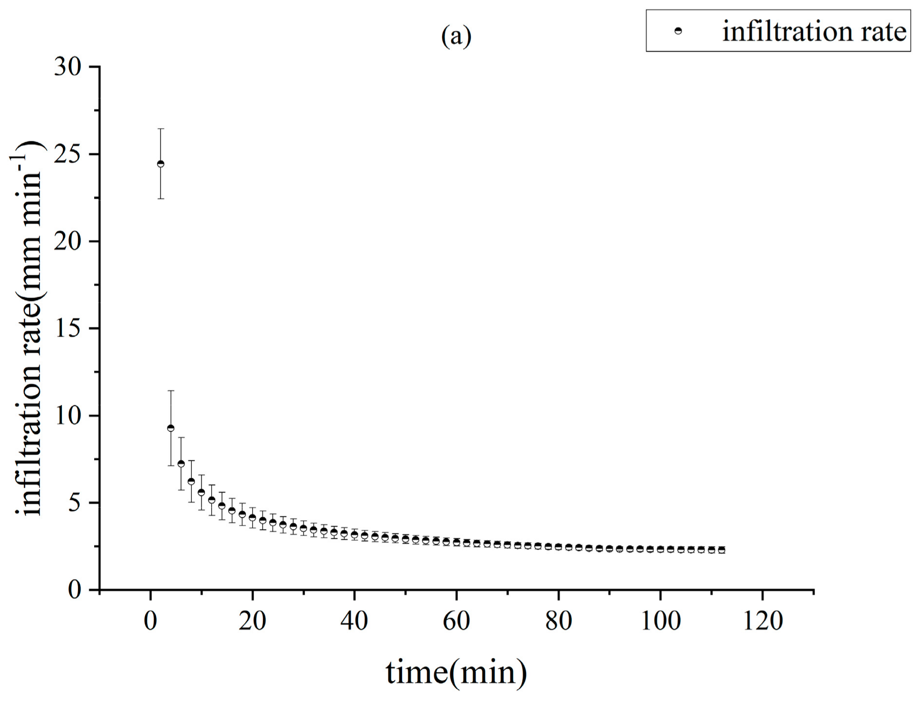
3.2. Estimation Results of Ks Using the Estimated Stable IR

The IR of each soil sample (Figure 8) was calculated using Equation (5). Initially, the IR reaches its peak because the soil is not yet saturated, thus allowing water to quickly penetrate into the deeper layers of the soil. As time progresses, the IR gradually decreases, and the speed of water infiltration slows down. When the soil becomes fully saturated, the IR stabilizes, meaning the soil can no longer absorb more water. We defined a threshold value of 0.1 mm min−1, and the soil IR was regarded as Ks when the slope of the IR curve was less than the threshold value. The estimated and measured Ks values are summarized in Table 4. The Ks of the humus samples from the cork oak stand and the oleander stand were 23.40 ± 1.21 mm min−1 and 23.86 ± 1.83 mm min−1, respectively, and the sandy loam was 22.99 ± 2.26 mm min−1. The soil texture and bulk density of the test soil column (19 cm long, 8 cm diameter) were the same as those of the drying test. The pressure head is set to 15 cm. When water flows out of the soil column at a constant rate, the increasing rate of the weight of the outgoing water as time elapsed was recorded, which was used to determine Ks. The Ks of the three soil samples calculated using Equation (11) were 24.41 ± 1.53 mm min−1, 24.26 ± 0.37 mm min−1, and 23.81 ± 0.10 mm min−1, respectively. The relative errors of the three soil samples between the two methods were 4.14%, 1.64%, and 3.42%, indicating that the NSIRM can accurately estimate Ks.

3.3. Estimation Results of the SWRC, AWC, and Ku

The optimized parameters α and n in the SWRC for each sample were inversely yielded when Equation (10) was minimized based on the comparisons between the simulated and measured θ (Figure 9a–c). Comparisons between the inverse-estimated and measured SWRC (Figure 9d–f) and the inverse estimation errors (Table 5) indicated that the proposed method is feasible for the inverse estimation of the SWRC.
The AWCs (Table 6) of the three soil samples were obtained from the SWRC. Based on the estimated Ks and SWRC, the results of the parameter estimation of the three soil samples using the inverse module are listed in Table 7.

4. Discussion

Among the current direct methods for estimating soil hydraulic properties, some require measuring ψ at two depths as well as soil evaporation to determine Ku [5,6,7,8,9], while others necessitate flow data measurements using a permeameter to determine Ks [19,20]. Additionally, there are methods that rely on a tensiometer to measure the soil suction and on θ to determine the SWRC [25,26]. However, these direct methods have drawbacks, such as extensive data requirements or the disruption of the soil structure. Like the underlying logic of this study, indirect methods like PTFs [27] estimate SHPs based on readily available soil information. However, research has identified up to 31 factors that can affect soil hydraulic properties (particle size distribution, hydraulic, morphological, and chemical properties) [39], indicating that this method requires numerous soil property parameters. Regardless of the method used, it only estimates a single SHP, and, if one aims to simultaneously obtain all SHPs, the required measurement data will accumulate further.
When compared to the traditional methods, the approach that combines sensors and data inversion retains the advantages of real-time monitoring, high accuracy precision, integration with automated systems, and the inherent labor savings of sensor-based measurement methods. Simultaneously, this approach harnesses the comprehensiveness and flexibility of data inversion, thus allowing the integration of diverse data sources and reducing the research costs. Specifically, this study only requires one soil infiltration experiment. Based on the easily obtainable θ and the estimated Ks, the parameters of the VG model can be inversely estimated, and then Ku can be estimated.
While this method can meet the practical measurement needs, it is still constrained by individual proficiency, and there are still some shortcomings. The collection of the soil wetting area requires manual handling, leading to a disconnection from the overall measurement process. The water supply arrangement for the linear infiltration method is also a manual operation, and the flow rate setting is cumbersome with inherent randomness. Additionally, this study is limited to laboratory measurements; in the future, point source experiments could be considered to extend the application of this method to field environments.

5. Conclusions

This study proposed a method for estimating near-surface SHPs using sensor-based soil infiltrability measurements and the inverse modeling of HYDRUS-2D. The near-surface soil infiltration rate was estimated using a linear source inflow method combined with an imaging processing method. The near-surface Ks was estimated using the stable infiltration rate. The estimated Ks values of two humus soil from the cork oak and oleander stands and one sandy loam from a farmland were 23.40 ± 1.21, 23.86 ± 1.83, and 22.99 ± 2.26 mm h−1, respectively. In comparison, the Ks of the three soil samples measured using the constant water head method were 24.41 ± 1.53, 24.26 ± 0.37, and 23.81 ± 0.1 mm h−1, respectively. The relative errors of the two methods were 4.14%, 1.64%, and 3.42%, respectively. The NRMSE of the SWRC for the three soil samples were 0.1724, 0.1454, and 0.0606, respectively. The AWC and Ku were also estimated based on these results. The method presented in this paper introduces a novel approach where SHPs can be obtained using just two devices, namely the image sensor and the moisture sensor, combined with the HYDRUS inversion module. In this process, data collected from the moisture sensor and the image sensor serve as input data for HYDRUS, and the output data from HYDRUS represent the estimated soil hydraulic properties. This represents a novel approach in the field, utilizing fewer devices that are integrated into a single apparatus, allowing for simultaneous data acquisition, while ensuring accuracy in estimation results. Further studies are needed to evaluate the performance of the proposed method under different soil classes.

Author Contributions

Conceptualization, X.Y., W.Z. and Q.C.; methodology, X.Y., W.Z., C.Z. and Q.C.; software, W.Z., Y.Z. and C.Z.; validation, W.Z. and Y.Z.; formal analysis, W.Z. and C.Z.; investigation, X.Y., W.Z., Y.Z. and C.Z.; resources, W.Z. and C.Z.; data curation, W.Z.; writing—original draft preparation, X.Y. and W.Z.; writing—review and editing, Q.C.; visualization, W.Z., Y.Z. and C.Z.; supervision, X.Y. and Q.C.; project administration, X.Y.; funding acquisition, X.Y. and Q.C. All authors have read and agreed to the published version of the manuscript.

Funding

This research was funded by the National Natural Science Foundation of China (Grant Nos. 31971576 and 32271990).

Data Availability Statement

The raw/processed data required to reproduce these findings cannot be shared at this time, as the data also form part of an ongoing study.

Conflicts of Interest

The authors declare no conflicts of interest.

References

  1. Virano-Riquelme, V.; Feger, K.-H.; Julich, S. Variation in Hydraulic Properties of Forest Soils in Temperate Climate Zones. Forests 2022, 13, 1850. [Google Scholar] [CrossRef]
  2. Archer, N.A.L.; Otten, W.; Schmidt, S.; Bengough, A.G.; Shah, N.; Bonell, M. Rainfall infiltration and soil hydrological characteristics below ancient forest, planted Forest and Grassland in a Temperate Northern Climate. Ecohydrology 2016, 9, 585–600. [Google Scholar] [CrossRef]
  3. Julich, S.; Kreiselmeier, J.; Scheibler, S.; Petzold, R.; Schwärzel, K.; Feger, K.H. Hydraulic properties of forest soils with stagnic conditions. Forests 2021, 12, 1113. [Google Scholar] [CrossRef]
  4. Archer, N.A.L.; Bonell, M.; MacDonald, A.M.; Coles, N. A Constant Head Well Permeameter Formula Comparison: Its Significance in the Estimation of Field-Saturated Hydraulic Conductivity in Heterogeneous Shallow Soils. Hydrol. Res. 2014, 45, 788–805. [Google Scholar] [CrossRef]
  5. Schindler, U. A rapid method for measuring the hydraulic conductivity in cylinder core samples from unsaturated soil. Arch. Agron. Soil Sci. 1980, 24, 1–7. [Google Scholar]
  6. Schindler, U.; Durner, W.; von Unold, G.; Müller, L. Evaporation method for measuring unsaturated hydraulic properties of soils: Extending the measurement range. Soil Sci. Soc. Am. J. 2010, 74, 1071–1083. [Google Scholar] [CrossRef]
  7. Schwen, A.; Zimmermann, M.; Bodner, G. Vertical variations of soil hydraulic properties within two soil profiles and its relevance for soil water simulations. J. Hydrol. 2014, 516, 169–181. [Google Scholar] [CrossRef]
  8. Peters, A.; Durner, W. Simplified evaporation method for determining soil hydraulic properties. J. Hydrol. 2008, 356, 147–162. [Google Scholar] [CrossRef]
  9. Peters, A.; Iden, S.C.; Durner, W. Revisiting the simplified evaporation method: Identification of hydraulic functions considering vapor, film and corner flow. J. Hydrol. 2015, 527, 531–542. [Google Scholar] [CrossRef]
  10. Tian, Z.; Kojima, Y.; Heitman, J.L.; Horton, R.; Ren, T. Advances in thermo-time domain reflectometry technique: Measuring ice content in partially frozen soils. Soil Sci. Soc. Am. J. 2020, 84, 1519–1526. [Google Scholar] [CrossRef]
  11. Xu, Q.; Zhu, Y.; Xiang, Y.; Yu, S.; Wang, Z.; Yan, X.; Du, T.; Cheng, Q. A novel frequency-domain integrated sensor for in-situ estimating unsaturated soil hydraulic conductivity. J. Hydrol. 2022, 610, 127939. [Google Scholar] [CrossRef]
  12. Burdine, N. Relative permeability calculations from pore size distribution data. J. Petrol. Technol. 1953, 5, 71–78. [Google Scholar] [CrossRef]
  13. Mualem, Y. A new model for predicting the hydraulic conductivity of unsaturated porous media. Water Resour. Res. 1976, 12, 513–522. [Google Scholar] [CrossRef]
  14. van Genuchten, M.T. A closed-form equation for predicting the hydraulic conductivity of unsaturated soils. Soil Sci. Soc. Am. J. 1980, 44, 892–898. [Google Scholar] [CrossRef]
  15. Šimůnek, J.; Angulo-Jaramillo, R.H.; Schaap, M.G.; Vandervaere, J.P.; van Genuchten, M.T. Using an inverse method to estimate hydraulic properties of crusted soils from tension-disc infiltrometer data. Geoderma 1988, 86, 61–81. [Google Scholar] [CrossRef]
  16. Šimůnek, J.; van Genuchten, M.T.; Wendroth, O. Parameter Estimation Analysis of the Evaporation Method for Determining Soil Hydraulic Properties. Soil Sci. Soc. Am. J. 1998, 62, 894–905. [Google Scholar] [CrossRef]
  17. Di Prima, S.; Lassabatère, L.; Bagarello, V.; Iovino, M.; Angulo-Jaramillo, R. Testing a new automated single ring infiltrometer for Beerkan infiltration experiments. Geoderma 2016, 262, 20–34. [Google Scholar] [CrossRef]
  18. Campbell, G.S. A simple method for determining unsaturated conductivity from moisture retention data. Soil Sci. 1974, 117, 311–314. [Google Scholar] [CrossRef]
  19. Reynolds, W.D.; Bowman, B.T.; Brunke, R.R.; Drury, C.F.; Tan, C.S. Comparison of tension infiltrometer, pressure infiltrometer, and soil core estimates of saturated hydraulic conductivity. Soil Sci. Soc. Am. J. 2000, 64, 478–484. [Google Scholar] [CrossRef]
  20. Reynolds, W.D.; Elrick, D.E. In-situ measurement of field-saturated hydraulic conductivity, sorptivity and the α-parameter using the Guelph permeameter. Soil Sci. 1985, 140, 292–302. [Google Scholar] [CrossRef]
  21. Klute, A.; Dirksen, C. Hydraulic conductivity and diffusivity: Laboratory methods. Methods of Soil Analysis: Part 1 Physical and Mineralogical. Methods 1986, 5, 687–734. [Google Scholar]
  22. Elrick, D.E.; Angulo-Jaramillo, R.; Fallow, D.J.; Reynolds, W.D.; Parkin, G.W. Infiltration under constant head and falling head conditions. Environmental mechanics: Water, mass and energy transfer in the biosphere. Geophys. Monogr. 2002, 129, 47–53. [Google Scholar]
  23. Rezaei, M.; Seuntjens, P.; Shahidi, R.; Joris, I.; Boënne, W.; Al-Barri, B.; Cornelis, W. The relevance of in-situ and laboratory characterization of sandy soil hydraulic properties for soil water simulations. J. Hydrol. 2016, 534, 251–265. [Google Scholar] [CrossRef]
  24. Bagarello, V.; Baiamonte, G.; Caia, C. Variability of near-surface saturated hydraulic conductivity for the clay soils of a small Sicilian basin. Geoderma 2019, 340, 133–145. [Google Scholar] [CrossRef]
  25. Mavroulidou, M.; Zhang, X.; Cabarcapa, Z. A study of the laboratory measurement of the soil water retention curve. In Proceedings of the 11th International Conference on Environmental Science and Technology 2009, Chania, Greece, 3–5 September 2009. [Google Scholar]
  26. Solone, R.; Bittelli, M.; Tomei, F.; Morari, F. Errors in water retention curves determined with pressure plates: Effects on the soil water balance. J. Hydrol. 2012, 470–471, 65–74. [Google Scholar] [CrossRef]
  27. Adnane, B.; Wilfred, O.; Ho-Chul, S.; Hannah, V.C.; Jane, R.; Aziz, S.; Mohamed, E.G. Evaluation of pedotransfer functions to estimate some of soil hydraulic characteristics in North Africa: A case study from Morocco. Environ. Sci. 2023, 11, 1090688. [Google Scholar]
  28. Šimůnek, J.; Van Genuchten, M.T.; Šejna, M. The HYDRUS Software Package for Simulating Two- and Three-Dimensional Movement of Water, Heat, and Multiple Solutes in Variably-Saturated Media; Technical Manual, Version 1.0; PC Progress: Prague, Czech Republic, 2006; Volume 1, p. 241. [Google Scholar]
  29. Sixtine, C.; Yves, C.; Jean-Noël, A.; Liliane, B.; Valérie, P.; Lionel, A. Estimation of soil water retention in conservation agriculture using published and new pedotransfer functions. Soil Tillage Res. 2021, 209, 104967. [Google Scholar]
  30. Sara, E.A.; Sofia, I.M.; Cristina, P.C.; Carlos, A.B. Effect of data availability and pedotransfer estimates on water flow modelling in wildfire-affected soils. J. Hydrol. 2023, 617, 128919. [Google Scholar]
  31. Assouline, S.; Or, D. The concept of field capacity revisited: Defining intrinsic static and dynamic criteria for soil internal drainage dynamics. Water Resour. Res. 2014, 50, 4787–4802. [Google Scholar] [CrossRef]
  32. Liu, H.; Rezanezhad, F.; Lennartz, B. Impact of land management on available water capacity and water storage of peatlands. Geoderma 2022, 406, 115521. [Google Scholar] [CrossRef]
  33. Veihmeyer, F.J.; Hendrickson, A.H. Methods of measuring field capacity and permanent wilting point. Soil Sci. 1949, 68, 75–94. [Google Scholar] [CrossRef]
  34. Costantini, E.A.C.; Pellegrini, S.; Bucelli, P.; Barbetti, R.; Campagnolo, S.; Storchi, P.; Magini, S.; Perria, R. Mapping suitability for Sangiovese wine by means of delta C-13 and geophysical sensors in soils with moderate salinity. Eur. J. Agron. 2010, 33, 208–217. [Google Scholar] [CrossRef]
  35. Ibrahimi, K.; Alghamdi, A.G. Available water capacity of sandy soils as affected by biochar application: A meta-analysis. CATENA 2022, 214, 106281. [Google Scholar] [CrossRef]
  36. Mao, L.L.; Lei, T.W.; Li, X.; Liu, H.; Huang, X.F.; Zhang, Y.N. A linear source method for soil infiltrability measurement and model representations. J. Hydrol. 2008, 353, 49–58. [Google Scholar] [CrossRef]
  37. Cui, Z.; Wu, G.L.; Huang, Z.; Liu, Y. Fine roots determine soil infiltration potential than soil water content in semi-arid grassland soils. J. Hydrol. 2019, 578, 124023. [Google Scholar] [CrossRef]
  38. Yu, S.; Xu, Q.; Cheng, X.; Xiang, Y.; Zhu, Y.; Yan, X.; Wang, Z.; Du, T.; Wu, X.; Cheng, Q. In-situ determination of soil water retention curves in heterogeneous soil profiles with a novel dielectric tube sensor for measuring soil matric potential and water content. J. Hydrol. 2021, 603, 126829. [Google Scholar] [CrossRef]
  39. Rawls, W.J.; Gish, T.J.; Brakensiek, D.L. Estimating soil water retention from soil physical properties and characteristics. Adv. Soil Sci. 1991, 16, 213–234. [Google Scholar]
Figure 1. (a) Variations in soil wetting area and infiltration rate and (b) the soil infiltration rate curves as a function of time at three different points in a horizontal position.
Forests 15 00569 g001
Figure 2. Schematic pictures of the measuring system at (a) the upper positive and (b) the upper right positions.
Forests 15 00569 g002
Figure 3. Diagram and photograph of the redesigned sensor probe for measuring the moisture content of the soil vertical profile at 1 cm intervals.
Forests 15 00569 g003
Figure 4. Flowchart for estimating the near-surface SHPs.
Forests 15 00569 g004
Figure 5. Schematic picture of the device for determining saturated soil hydraulic conductivity.
Forests 15 00569 g005
Figure 6. Image processing: original image (a,b,d), distortion correction (c,e), and binarization (f).
Forests 15 00569 g006
Figure 7. Variations in the averaged wetted areas of the three soil samples from the cork oak stand (a), oleander stand (b), and sandy loam (c).
Forests 15 00569 g007
Figure 8. Variations in the infiltration rate (IR) of the three soil samples from the cork oak stand (a), oleander stand (b), and sandy loam (c).
Forests 15 00569 g008aForests 15 00569 g008b
Figure 9. Estimated and measured θ and SWRC from the cork oak stand (a,d), oleander stand (b,e), and sandy loam farmland (c,f), respectively.
Forests 15 00569 g009
Table 1. The relations and R2 values in the different soil samples: the humous soil from both the cork oak (Quercus suber L.) and oleander (Pinus tabuliformis L.) stands, and the sandy loam from the farmland. In which “y” represents the soil moisture content and “x” represents the output voltage value of the moisture sensor.
Soil SamplesRelationsR2
Humus soilCork oak stand y = 22.692 x 3 27.274 x 2 + 11.809 x 1.7261 0.9898
Oleander stand y = 7.5084 x 3 + 10.08 x 2 2.8212 x + 0.1402 0.9986
Sandy loamFarmland y = 186.67 x 4 + 383.46 x 3 2877.77 x 2 + 94.603 x 11.533 0.9887
Table 2. Physical properties of the experimental soil samples.
Soil TextureDepth (cm)Initial Moisture Content (%)Sand (%)Silt (%)Clay
(%)
Organic Matter Content (%)Bulk Density
(g cm3)
Porosity
(%)
Humus soilCork oak stand0–101.42///8.351.1855.47
Oleander stand22.9314.951.07159.58
Sandy loamFarmland2.8339.946.613.51.851.3350.19
Table 3. Regression equations between the wetting area and time of the three soil samples.
Soil Samples Wetting   Area   ( m m 2 )R2
Humus soilCork oak stand A = 5.93 × 1 0 2 4.848 × 1 0 2 e 0.02265 t 0.9938
Oleander stand A = 7.599 × 1 0 2 5.226 × 1 0 2 e 0.02204 t 0.9947
Sandy loamFarmland A = 7.146 × 1 0 2 5.724 × 1 0 2 e 0.02438 t 0.9988
Table 4. Results of Ks as measured using the CHM and NSIRM.
Soil TextureConstant Head Standard
(mm min−1)
Linear Source Inflow
(mm min−1)
Relative Error
(%)
Humus soilCork oak stand24.41 ± 1.5323.40 ± 1.214.14
Oleander stand24.26 ± 0.3723.86 ± 1.831.64
Sandy loamFarmland23.81 ± 0.1022.99 ± 2.263.42
Table 5. NRMSE of the simulated and measured θ and SWRC of the three soil samples.
Soil TextureNRMSE of Soil Water Content (θ)NRMSE of SWRCAveraged NRMSE of SWRC
Humus soilCork oak standFirst0.19580.14890.1724
Second0.19470.1597
Third0.20190.2086
Oleander standFirst0.12160.12090.1454
Second0.14710.1286
Third0.16880.1867
Sandy loamFarmlandFirst0.13370.06720.0606
Second0.15520.0726
Third0.15420.0421
Table 6. AWC of the three soil samples.
Soil TextureField Capacity (FC)Permanent Wilting Point (PWP)Available Water Capacity (AWC)Average of AWC
Humus soilCork oak standFirst0.02270.0160.00670.0058
Second0.01660.0150.0016
Third0.02210.0130.0091
Oleander standFirst0.40310.06760.33550.307
Second0.35720.05340.3038
Third0.32740.04570.2817
Sandy loamFarmlandFirst0.30620.04220.2640.221
Second0.30620.1130.1932
Third0.3140.10830.2057
Table 7. Parameter identification results of the three soil samples.
Soil TextureθrθsαnKs (mm min−1)l
Humus soilCork oak stand0.01470.4600.09865.075723.400.5
Oleander stand0.02000.4860.03571.649623.860.5
Sandy loamFarmland0.01260.3400.01771.512722.990.5
Disclaimer/Publisher’s Note: The statements, opinions and data contained in all publications are solely those of the individual author(s) and contributor(s) and not of MDPI and/or the editor(s). MDPI and/or the editor(s) disclaim responsibility for any injury to people or property resulting from any ideas, methods, instructions or products referred to in the content.

