Addressing Carbon Storage in Forested Landscape Management Planning—An Optimization Approach and Application in Northwest Portugal

Abstract

Climate change is driving worldwide efforts to mitigate and reverse the increasing anthropogenic emissions of greenhouse gases. Forests can uptake considerable amounts of carbon from the atmosphere, but management decisions and resultant silvicultural practices can largely influence these ecosystems’ carbon balance. This research presents an approach to help land managers cope with the need to ensure the provision of forest products and services while contributing to mitigating climate change via carbon sequestration. The emphasis is on combining a landscape-level resource capability model with a mathematical programming (LP) optimization method to model and solve a land management problem involving timber production, carbon sequestration, and resistance to wildfire targets. The results of an application on a forested landscape in Northwest Portugal showed that this approach may contribute to analyzing and discussing synergies and trade-offs between these targets. They revealed important trade-offs between carbon sequestration and both timber production and fire resistance.

1. Introduction

Emissions of the principal greenhouse gas (GHG), carbon dioxide (CO₂), are driven primarily by the burning of fossil fuels, but the Earth’s biosphere also plays a major role in the global carbon (C) budget [1]. Globally, terrestrial ecosystems are currently a major net sink for atmospheric CO₂; this sink mostly represents the difference between C accumulation in forests and CO₂ emissions from tropical deforestation [2]. Forests play a crucial role in sequestering and sinking CO₂ and also regulate the future rate of increase in atmospheric CO₂ depending on their management and dynamics. Properly managing and preserving forests can significantly contribute to carbon storage and help reduce the impacts of climate change. The management of forests for this purpose is receiving increased attention from national and global policymakers.

Forests offer possibilities to sequestrate carbon in living biomass, deadwood, and forest soils, as well as in products prepared of wood [3,4,5] and also non-wood forest products [6,7]. In most forests, the largest C pools are aboveground live biomass and mineral soil organic matter, with lesser amounts in roots and litter. The rate at which C accumulates in the ecosystem—net ecosystem productivity (NEP)—represents the sum of changes in each of these pools. Biologically, NEP is the difference between net primary productivity (NPP, the annual net carbon fixation by plant photosynthesis) and heterotrophic respiration (CO₂ emission by non-photosynthetic organisms). Both NEP and the size of these C pools are highly sensitive to forest management activities. The most rapidly changing pool is usually aboveground live biomass, which can be estimated accurately through allometric approaches [8,9,10]. Accurately quantifying changes in the other C pools (e.g., soil, dead trees) is more difficult considering the complex and dynamic nature of ecosystems. The spatial and temporal variability, as well as the diversity of ecosystems and their responses to environmental factors, pose challenges.

Modeling approaches to forest growth and management are used to represent the process of growth and harvesting of the forest as the flow through a network that can be classified into two approaches [11], known as models I and II. The main difference lies in the level of aggregation on the treatments performed in each arc of the flow network. The most commonly used is model I where each arc is a complete set of silvicultural treatments for a management unit (stand) or an aggregation of management units, covering the entire duration of the planning horizon. The decision variables represent a sequence of actions on a given forest unit for the entire planning period. In model II, individual parcels of land are not kept intact through time. Here, activity refers to a complete set of actions that can occur on a particular land area from the time the area is regenerated until it is regeneration harvested, or until it is left as ending inventory at the end of the planning horizon [12,13,14,15]. The choice between the two models depends on the specific objectives, scope, and level of detail required for a particular forest management scenario.

Strategic forest management models are largely used to design and maintain existing carbon stocks and maximize capacity for future sequestration. These models can help identify underused opportunities to increase forest carbon stocks without diminishing other forest products [3,16,17,18,19,20,21]. These models have been used to decide on the annual volumes of timber that can be harvested on a sustainable basis within defined forest areas and the types of management actions or silvicultural treatments for regenerating the harvested forest (what treatments, in which stand types, and when to carry them out), e.g., [22,23,24,25]. By using species-specific biomass equations, developed at a regional or country level and based on common forest inventory biometric variables and biophysical information, we expected to (i) easily and systematically estimate forested landscapes’ C stocks, corresponding to different pools; (ii) be able to compare results for a wide range of management alternatives; and (iii) ultimately select the best one, towards landscape C stock potential, by incorporating this information into a resource capability model to be read by a linear programming-based optimization tool. We hypothesize that trade-offs will become evident, between the main goal of C stock and other important ecosystem services, such as the demand for wood production or resistance to wildfire.

2. Materials and Methods

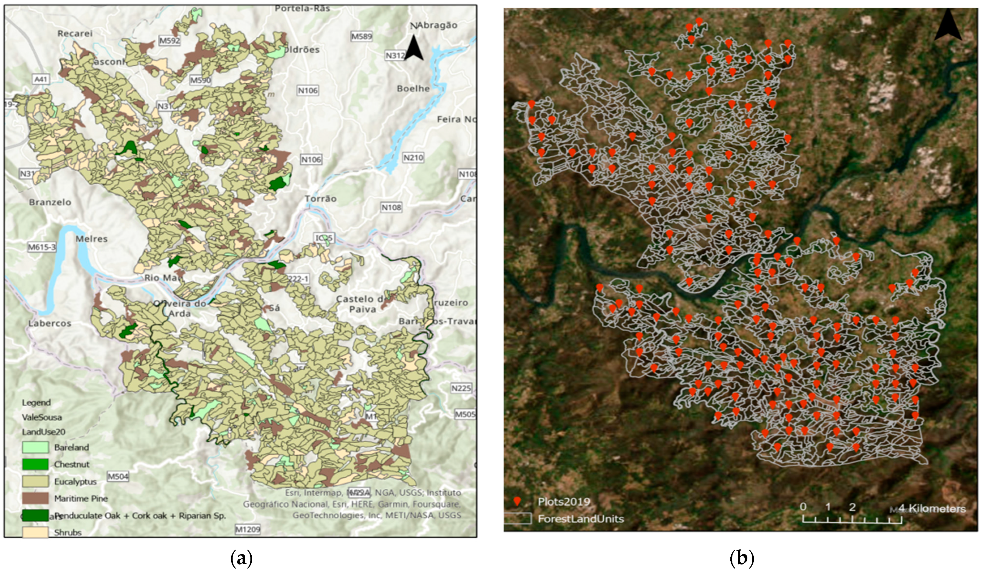
2.1. Case Study Characterization

For testing purposes, a forested area with about 14,320 ha located in the Vale do Sousa area was considered. It is located in part of Paredes and Penafiel counties, north of Douro River, and to the south, Castelo de Paiva county (Figure 1a). The area was inventoried with 155 plots (Figure 1b) from August to November 2019 and species composition was recorded as well as understory vegetation. The forest inventory data collected included the diameter breast height (dbh, cm) and tree height (h, m). These data allowed the characterization of the stands, by the computation of the stand’s tree density (number of trees per ha, Nt, ha⁻¹), and other associated stand variables such as standing volume and biomasses of the different tree components.

Currently, the area (Figure 1 and

Table 1. Land use characterization for 14,320 hectares of forest land in Vale do Sousa, inventoried in 2020.

Land Use	Species	N. of Stands	Area (ha)
Bare or shrubland	-	251	2343.4
Pure	Eucalyptus globulus Labill.	920	9990.5
	Pinus pinaster Aiton.	85	751.4
	Riparian sp.	41	108.6
	Quercus suber L.	1	12.8
	Castanea sativa Mill.	1	2.3
Mixed	E. globulus L. and P. pinaster A.	64	615.2
	E. globulus L. and Q. suber L.	4	69.8
	P. pinaster A. and E. globulus L.	38	416.2
	P. pinaster A. and Q. suber L.	1	2.3
Total		1406	14,320

) is mainly dominated by pure stands of eucalyptus (Eucalyptus globulus Labill.), which occupy about 70% of the area, followed by pure stands of maritime pine (Pinus pinaster Aiton.), accounting for 5%. It was also observed that mixed stands, namely Eucalypt globulus Labill and Pinus Pinaster Aiton., represent 8% of the total area. Near the Douro River and its confluent rivers and streams, there is a presence of riparian species such as Alnus glutinosa (L.) Gaertn., Salix atrocinera Brot, Salix alba L., Fraxinus angustifolia Vahl., and Populus nigra L. Due to recent wildfires and recent clearcuts, 16% of the forest area was classified as bare land or occupied by shrubs. Understorey vegetation is mainly composed of Erica sp., Cistus ladanifer L., Ulex sp., Adenocarpus angyrophyllus Caball., Rubus fruticosus L., and Quercus lusitanica Lam. A residual area, about 0.1% comprising hardwoods, namely chestnuts (Castanea sativa Mill.) and cork oak (Quercus suber L.), is present.

2.2. Forest Growth Projections

Forest growth was assessed via specific empirical growth and yield models over a planning horizon of 100 years, allowing us to estimate the evolution of wood production volumes originated by thinnings, and accounting with different assortments of biomass and carbons.

Each prescription is a schedule of silvicultural activities (e.g., planting, thinning, regeneration, fertilization, or harvesting), which when implemented on a stand is expected to achieve the desired outcomes. Usually, a myriad of different prescriptions is technically or biologically possible for each stand and were then simulated using species-specific empirical growth and yield models or yield tables (Figure 2 and

Table 2. Forest species and simulated prescriptions for the CSA.

Silvicultural Operations	Units	E. globulus	P. pinaster	C. sativa	Q. robur	Q. suber	Riparian Spp.
Plantation density (a)	N.trees/ha	1400	1111	1250	1600	833	5000
Replanting (b,c)	%		-	-	20	20	-
Stool selection (d,e)	N. of stools/stump	2	-	-	-	-	-
Prunning (f)	Age	-	-	-	23	-	-
Pre-commercial thinning	Age	-	15	-	-	-	-
Thinning (g)	Age	-	25 to 45 (10)	Alternative periodicities (5 to 10) starting at 15	27, 37, 45	15, 30, 40, 58, 76	-
Wilson Factor	-	-	0.27	-	0.2	-	-
Debarking (h)	Age	-	-	-	-	30, 40, (+9)	-
Final harvest (i,j)	Age	10 to 12 (1)	35 to 50 (5)	40 to 55 (5)	40 to 70 (10) and 120	-	-

^(a) Number of plants per ha; ^(b) one year after the plantation; ^(c) in percentage; ^(d) only applicable to eucalyptus; ^(e) in cycles 2 and 3 after 3 years; ^(f) only applicable to pedunculate oak; ^(g) parentheses ( ) show the interval between thinnings; ^(h) only applicable to cork oak; parentheses ( ) show the interval between debarkings; ⁽ⁱ⁾ clear-cuts; parentheses ( ) show interval for harvests; ^(j) cork oaks are only allowed upon forest service authorization.

). The Globulus 3.0 [26] and the Pinaster [27,28] models, both implemented in the standsSIM-MD module included in the SIMFLOR platform (Lisbon, Portugal) [29], were used for E. globulus and P. pinaster, respectively. The SUBER v5.0 [30,31,32], implemented in the same platform [33], was used for the growth simulation of Q. suber. The SimGaliza simulator [34,35], developed for Q. robur stands in Galicia (Spain), was also used, considering the similar soil and climate conditions from that region and our case study area. For C. sativa, the yield tables proposed by [15,16] were used. We obtained, from riparian stand national databases [36,37], structural parameters over the planning horizon.

The stakeholders from Vale do Sousa have identified forest species that are not currently present in the area, and which they plan to have in the near future. So, in our prescription list, we considered the possibility of species conversion. The complete set of prescriptions was matched to the landscape management units, according to their biophysical aptitude (e.g., soil type and depth, altitude) and location (policy regulations). When a conversion to a new management model was a possibility, it was scheduled to occur in the year of the first clearcut harvest of the current species. As a result, most of the area was considered suitable for P. pinaster plantations, both pure and mixed (92% of the landscape); C. sativa, Q. robur, and Q. suber alternative management models were considered for nearly 46% of the landscape.

For each prescription, the shrub biomass accumulation (Mg ha⁻¹) under canopy cover was projected [38] considering different fuel treatment schedule options (no fuel treatment, 5 years, and 10 years) applied over the whole planning horizon. Fuel removal prescriptions are carried out manually or mechanically in the understory vegetation, considering the slope and other site restrictions. The simulation of each prescription allowed the estimation of the evolution of wood volumes, biomass, and carbon pools, including the values removed as a result of thinning or final-cut silviculture operations.

2.3. Forest Carbon Pools Estimations

For every forest stand and considered management prescriptions, tree standing and harvested C pools—including stem (Ws), bark (Wb), branches (Wbr), leaves (Wl), and roots (Wr), as well as cork (Wc) for Q. suber, using available national or regional species-specific biomass equations, multiplied by respective C percentage of dry matter (

Table 3. Literature references for the considered species-specific biomass equations and carbon fractions.

Species	Biomass and Root Ratios References	% C—Adapted from [39]
Castanea sativa Mill.	[39,40,41] for roots	48.4 [39]
Eucalyptus sp. Labill	[26]	47.5 [39]
Pinus pinaster Ait.	[27,42]	51.1 [39]
Quercus robur L.	[34,35,42]	48.4 [39]
Quercus suber L.	[31,43]	47.2 [39]
		60.0 virgin cork: 55.0 reproduction cork [39]

). Biomass models for both C. sativa and Q. robur root biomass were not available, so root ratios of 49 and 20%, respectively, were applied.

Except for plantation, which is assumed to occur at the beginning of the year, all other silviculture operations, including, pruning, thinning, shrub clearing, cork or resin extraction, and clear-cut harvesting, were considered to take place at the end of the year defined in the prescription, carbon stocks being reported afterward.

Understory shrub biomass was estimated following the approach of ref. [38], and the respective C content was obtained using a 0.50 carbon conversion factor, in agreement with IPCC guidelines [44].

2.4. Other Ecosystem Services Estimations

Wood → The amount of wood standing or removed from the forest through thinning or clearcuts is a direct output from the growth and yield simulators.

Fire Resistance indicator → Each management unit fire resistance was calculated following the approaches of refs. [18,19], which encompass not only management-related biometric variables to model wildfire occurrence and damage but also neighboring stand characteristics’ impacts on wildfire probability and spread [45]. The resultant stand-level values were weighted and averaged for the whole landscape and scaled from 0 to 5; for better understanding, 1 represents the lowest fire resistance and 5 represents the highest fire resistance.

Erosion → The soil erosion computation was computed following the approach proposed by [24].

2.5. Resource Capability Model Building

A total of 84,275 prescriptions—approximately 194 management alternatives per stand, on average—were used to build a resource capability model (RCM), model I, that is described by Equations (1)–(28).

$${\sum }_j^{N_i}{x}_{ij}=1i=1,\dots ,M;j=1,\dots ,N_i$$

(1)

$${\sum }_i^M{\sum }_{{j\in SPECIES}_s}^N{a}_i{x}_{ij}=A_{{SPECIES}_s}s=1,\dots ,S$$

(2)

$$\raisebox{1ex}{$({\sum }_i^M{\sum }_j^N{ctreestanding}_{ijt}{x}_{ij}+{\sum }_i^M{\sum }_j^N{cshrubstanding}_{ijt}{x}_{ij})$}\!\left/ \!\raisebox{-1ex}{$Area$}\right.={Cstanding}_t,t=1,\dots ,T$$

(3)

$$\raisebox{1ex}{${\sum }_i^M{\sum }_j^N{ctreestanding}_{ijt}{x}_{ij}$}\!\left/ \!\raisebox{-1ex}{$Area$}\right.={Ctreestanding}_t,t=1,\dots ,T$$

(4)

$$\raisebox{1ex}{${\sum }_i^M{\sum }_j^N{cshrubstanding}_{ijt}{x}_{ij}$}\!\left/ \!\raisebox{-1ex}{$Area$}\right.={Cshrubstanding}_t,t=1,\dots ,T$$

(5)

$$\raisebox{1ex}{${\sum }_i^M{\sum }_j^N{ctreeharvested}_{ijt}{x}_{ij}$}\!\left/ \!\raisebox{-1ex}{$Area$}\right.={Ctreeharvested}_t,t=1,\dots ,T$$

(6)

$$\raisebox{1ex}{${\sum }_i^M{\sum }_j^N{cshrubharvested}_{ijt}{x}_{ij}$}\!\left/ \!\raisebox{-1ex}{$Area$}\right.={Cshrubharvested}_t,t=1,\dots ,T$$

(7)

$$\raisebox{1ex}{$({\sum }_i^M{\sum }_j^N{ctreeharvested}_{ijt}{x}_{ij}+{\sum }_i^M{\sum }_j^N{cshrubharvested}_{ijt}{x}_{ij})$}\!\left/ \!\raisebox{-1ex}{$Area$}\right.={Cremoved}_t,t=1,\dots ,T$$

(8)

$${\sum }_i^M{\sum }_j^N{fra}_{ijt}{x}_{ij}={FRA}_{t}t=1,\dots ,T$$

(9)

$${\sum }_i^M{\sum }_j^{N_i}{erosion}_{ijt}{x}_{ij}={Erosion}_{t}t=1,\dots ,T$$

(10)

$${\sum }_i^M{\sum }_j^N{pinus}_{ijt}{x}_{ij}={Vpinus}_{t}t=1,\dots ,T$$

(11)

$${\sum }_i^M{\sum }_j^N{eucalypt}_{ijt}{x}_{ij}={Veuc}_{t}t=1,\dots ,T$$

(12)

$${\sum }_i^M{\sum }_j^N{castanea}_{ijt}{x}_{ij}={Vcast}_{t}t=1,\dots ,T$$

(13)

$${\sum }_i^M{\sum }_j^N{qrobur}_{ijt}{x}_{ij}={Vqrob}_{t}t=1,\dots ,T$$

(14)

$${\sum }_i^M{\sum }_j^N{qsuber}_{ijt}{x}_{ij}={Vqsub}_{t}t=1,\dots ,T$$

(15)

$${Vpinus}_t+{Veuc}_t+{Vcast}_t+{Vqrob}_t+{Vqsub}_t+{Vrip}_t={VEI}_{t}t=1,\dots ,T$$

(16)

$${\sum }_i^M{\sum }_j^N{wpinus}_{ijt}{x}_{ij}={Wpinus}_{t}t=1,\dots ,T$$

(17)

$${\sum }_i^M{\sum }_j^N{weucalypt}_{ijt}{x}_{ij}={Weuc}_{t}t=1,\dots ,T$$

(18)

$${\sum }_i^M{\sum }_j^N{wcastanea}_{ijt}{x}_{ij}={Wcast}_{t}t=1,\dots ,T$$

(19)

$${\sum }_i^M{\sum }_j^N{wqrobur}_{ijt}{x}_{ij}={Wqrob}_{t}t=1,\dots ,T$$

(20)

$${\sum }_i^M{\sum }_j^N{wqsuber}_{ijt}{x}_{ij}={Wqsub}_{t}t=1,\dots ,T$$

(21)

$${Wpinus}_t+{Weuc}_t+{Wcast}_t+{Wqrob}_t+{Wqsub}_t={Wood}_{t}t=1,\dots ,T$$

(22)

$${\sum }_1^T\raisebox{1ex}{${Cstanding}_t$}\!\left/ \!\raisebox{-1ex}{$T$}\right.=CStock$$

(23)

$${\sum }_1^T{Cremoved}_t=CRemoved$$

(24)

$${\sum }_1^T\raisebox{1ex}{${FRA}_t$}\!\left/ \!\raisebox{-1ex}{$T$}\right.=FRA$$

(25)

$${\sum }_1^T{Erosion}_t=Erosion$$

(26)

$${\sum }_1^T{Wood}_t=Wood$$

(27)

$$0\le x_{ij}\le 1\forall i,j$$

(28)

where x_ij are the decision variables, representing the proportion of management unit i area under prescription j (varying from 0 to 1); M is the number of management units (1406); N_i is the number of possible prescriptions for each stand i; a_i is the area of management unit i; S is the number of forest species (6); SPECIES_s is the set of prescriptions j that correspond to species s; cstanding_ijt is the annual average standing carbon in the forest (Mg ha⁻¹) in period t, resulting from assigning to stand i prescription j; Area is the total landscape area (14,320 ha); T is the number of planning periods (10); ctreestanding_ijt is the average annual carbon standing in trees (Mg ha⁻¹) in period t, that results from allocating prescription j to stand i; cshrubstanding_ijt is the yearly average carbon standing in shrubs biomass (Mg ha⁻¹) in period t, resulting from choosing prescription j for stand i; ctreeharvested_ijt is the total carbon harvested as tree products along period t, as a result of assigning prescription j to stand i; cshrubharvested_ijt is the total carbon harvested in shrubs biomass along period t, as a result of assigning prescription j to stand i; fra_ijt is the fire resistance indicator in period t that results from assigning prescription j to stand i; erosion_ijt is the potential soil loss in Mg in period t, resulting from assigning to stand i prescription j; pinus_ijt, eucalypt_ijt, castanea_ijt, qrobur_ijt and qsuberk_ijt are, respectively, P. pinaster, E. globulus, C. sativa, Q. robur and Q. suber, standing volumes at the end of period t, associated with prescribing management alternative j to stand i; wpinus_ijt, weucalypt_ijt, wcastanea_ijt, wqrobur_ijt and wqsuber_ijt are, respectively, the harvested wood volumes of P. pinaster, E. globulus, C. sativa, Q. robur and Q. suber, which result from assigning prescription j to stand i along period t.

Equation (1) requires that all areas in a stand (a_i) must be managed so that the sum of all area proportions (x_ij) assigned to all prescriptions j, for every management unit i, must be equal to one. Equations (2)–(27) estimate the values of bookkeeping variables reflecting the problem resource capability model. The areas assigned to each forest species (A_SPECIESs) are accounted for by Equation (2). Equations (3)–(5) express the annual average value of forest standing carbon per hectare, in the trees (Ctreestanding_t), the shrubs (Cshrubstanding_t), and both (Cstanding_t) within each 10-year planning period t. Equation sets (6) and (7) account for the total harvested carbon from the products of the tree (Ctreeharvested_t) and the understorey shrubs layer (Cshrubharvested_t) per hectare and planning period t. The landscape fire resistance in each period t is computed as FRA_t through Equation (9). Potential soil losses for each period t are defined by accounting variables Erosion_t (Equation (10)). Equation sets from (11) to (15) account for the landscape standing volume for each tree species and period (t), while Equation (16) calculates the total landscape standing volume at the end of each planning period (VEI_t). Equation sets from (17) to (21) define the harvested wood volume of each species, obtained within each 10-year period, and Equation (22) represents the total landscape timber yield for each t (Wood_t). The variables defined by Equations (23) and (27) express the landscape average standing carbon (Carbon) that belong to the tree pool (Carbontree) and shrub layer (Carbonshrub), total harvested carbon from the trees (Carbonharvestedtree) and shrubs (Carbonharvestedshrub), average fire resistance (FRA), accumulated soil losses (Erosion), and total wood production (Wood), respectively, along the 100-year planning horizon. Non-negativity constraints are represented by the set of inequalities expressed by Equation (28).

Two scenarios were analyzed: the expansion of the cork oak area (ExpQS): the area of Q. suber is allowed to increase; and business as isual (BAU): the area of Q. suber will be maintained during the planning horizon. The models were used also for optimizing soil protection while demanding a minimum timber supply, defined with a 12-million-cubic-meter threshold for harvested wood along the 100-year planning horizon (Equation (29)). In addition, a constraint was used that imposed a minimum fire resistance value of 3.7 (Equation (30)).

$$\mathrm{W}\mathrm{o}\mathrm{o}\mathrm{d}\ge \mathrm{12,000,000}$$

(29)

$$\mathrm{F}\mathrm{R}\mathrm{E}\mathrm{S}\ge 3.7$$

(30)

The model was tested for the three contrasting objectives of timber provision (only without constraints; Equation (33)) and carbon stock and carbon removed (Equations (31) and (33)).

$$\mathrm{M}\mathrm{a}\mathrm{x}\mathrm{i}\mathrm{m}\mathrm{i}\mathrm{z}\mathrm{e} \mathrm{W}\mathrm{o}\mathrm{o}\mathrm{d}$$

(31)

$$\mathrm{M}\mathrm{a}\mathrm{x}\mathrm{i}\mathrm{m}\mathrm{i}\mathrm{z}\mathrm{e}/\mathrm{m}\mathrm{i}\mathrm{n}\mathrm{i}\mathrm{m}\mathrm{i}\mathrm{z}\mathrm{e} \mathrm{C}\mathrm{a}\mathrm{r}\mathrm{b}\mathrm{o}\mathrm{n} \mathrm{S}\mathrm{t}\mathrm{o}\mathrm{c}\mathrm{k}$$

(32)

$$\mathrm{M}\mathrm{a}\mathrm{x}\mathrm{i}\mathrm{m}\mathrm{i}\mathrm{z}\mathrm{e}/\mathrm{m}\mathrm{i}\mathrm{n}\mathrm{i}\mathrm{m}\mathrm{i}\mathrm{z}\mathrm{e} \mathrm{C}\mathrm{R}\mathrm{e}\mathrm{m}\mathrm{o}\mathrm{v}\mathrm{e}\mathrm{d}$$

(33)

The RCM was built and solved independently for the scenarios.

Table 4. Scenarios addressed in the study.

Alias		Objective Function	Constraints
Expansion of Qs Area	Business as Usual (BAU)
ExpQS_MaxW	BAU_MaxW	Max Wood	None
ExpQS_MaxCS	BAU_MaxCS	Max Cstock	None
ExpQS_MaxCR	BAU_MaxCR	Max Cremoved	None
ExpQS_MinCS	BAU_MinCS	MinCStock	None
ExpQS_MinCR	BAU_MinCR	MinCremoved	None
ExpQS_MaxCSW12	BAU_MaxCSW12	Max Cstock	Equation (29)
ExpQS_MaxCSFire	BAU_MaxCSFire	Max Cstock	Equation (30)

Where: Qs: Quercus suber L.

summarizes the problems addressed and the respective LP models and constraints analyzed.

3. Results

The models were solved via CPLEX Interactive Optimizer 12.5 (IBM, New York, NY, USA, 2013) on a computer equipped with an Intel Core i5 processor and 16 GB of RAM.

Currently, the forested landscape in Vale do Sousa is being managed to maximize the total amount of timber extracted from the forest. With this objective, the scenarios ExpQS_MaxW and BAU_MaxW were optimized. In both scenarios, 14.06 million m³ can be harvested in a 100-year planning horizon. The similar results in both scenarios are explained by the fact that the Q. suber exploration does not allow clearcuts within the planning horizon, but only cork extraction every 9 years after the first debark. The impact of the management plans with this objective on soil erosion and fire resistance are similar (

Table 5. Results from scenarios without constraints.

Alias	Cstock (×106 Mg)	Cremoved (×106 Mg)	Wood (×106 M3)	Erosion Mg/Ha/Year	Rait [0–5]
ExpQS_MaxW	35.65	576.73	14.06	88.08	3.11
BAU_MaxW	35.61	576.77	14.06	88.05	3.10
ExpQS_MaxCS	94.78	370.76	7.63	94.78	3.77
BAU_MaxCS	52.51	517.58	11.82	78.09	3.33
ExpQS_MaxCR	39.74	610.29	13.19	83.96	3.31
BAU_MaxCR	39.33	610.10	13.19	84.31	3.29
ExpQS_MinCS	8.78	94.92	6.79	79.58	2.38
BAU_MinCS	8.78	94.92	6.79	79.58	2.38
ExpQS_MinCR	10.21	85.31	7.61	82.51	2.21
BAU_MinCR	13.66	79.00	7.40	79.61	2.31

Cstock—carbon stock in the forest (14,316 ha); Cremoved—the total carbon removed in the landscape in 100 y planning horizon from the tree and shrub removals; Wood—the total wood removed (thinning + harvests). Bold shows the optimal value according to the objective function.

). Also, the same trend was found when analyzing the amount of carbon storage and the total amount removed.

If the stakeholders and the entity that manages the forest want to optimize the amount of carbon storage by solving models ExpQS_MaxCS and BAU_MaxCS, it is possible to obtain 94.78 and 52.51 million Mg, respectively. In the scenario, characterized by Q. suber expansion, the amount of total wood removed was reduced to 7.63 × 10⁶ M³, prioritizing prescriptions with longer rotations (e.g., C. sativa and Q. suber). On the other hand, in the BAU scenario, the amount of wood removed was higher, namely 11.82 × 10⁶ M³, mostly from E. globulus stands, C. sativa, and P. pinaster. Scenarios leading to an optimum level of removed carbon, from tree harvesting, thinning, shrub cleaning, and debarking, had similar results regarding the five criteria analyzed. Yet, a deeper analysis of the results revealed that the prescriptions assigned to each management unit were mostly very short rotations (e.g., 10 years for E. globulus with a shrub cleaning periodicity of 5 years).

Regarding tree species distribution on the landscape (

Table 6. Area occupied (in hectares) by each species in each scenario.

	Without Constraints
Specie	Pp	Eg	Cs	Qr	Qs	Rp
ExpQS_MaxW	2488.9	11,340.6	312.8	0.0	65.2	108.6
BAU_MaxW	2496.5	11,340.6	316.1	0.0	54.32	108.6
ExpQS_MaxCS	1377.9	3794.3	1179.2	0.0	7856.1	108.6
BAU_MaxCS	2360.7	8476.4	3316.1	0.0	54.3	108.6
ExpQS_MaxCR	2088.6	10,006.6	1970.2	0.0	142.1	108.6
BAU_MaxCR	2176.3	10,006.6	1970.2	0.0	54.3	108.6
ExpQS_MinCS	12,641.9	686.4	5.5	819.3	54.3	108.6
BAU_MinCS	12,641.9	686.4	5.5	819.3	54.3	108.6
ExpQS_MinCR	12,482.3	408.9	5.5	587.5	723.3	108.6
BAU_MinCR	13,105.5	454.7	5.5	587.5	54.3	108.6
	With Constriants
ExpQS_MaxCSW12	1636.2	7647.7	776.3	0.0	4147.3	108.6
BAU_MaxCSW12	2300.6	8551.9	3300.6	0.0	54.3	108.6
ExpQS_MaxCSFire	1377.9	3794.3	1179.2	0.0	7856.1	108.6
BAU_MaxCSFire	2318.8	8518.3	3316.1	0.0	54.3	108.6

Pp—Pinus pinaster Aiton., Eg—Eucalyptus globulus Labill., Cs—Castanea sativa L. Qr—Quercus robur L., Qs—Quercus suber L., and Rp—Riparian species.

), model solutions for two scenarios were shown to be slightly different according to the different objective functions (Figure 3). The results showed that, for timber maximization purposes, a bigger proportion of the landscape should be occupied by E. globulus plantations (79.2%) in both scenarios (BAU with Q. suber expansion), followed by P. pinaster with an occupation of 17.4% of the CSA area. The remaining area will be occupied by broadleaves, mainly C. sativa.

A maximum level of carbon stock was achieved (94.78 × 10⁶ M³) for the case study area in the scenario ExpQS_MaxCS, where Q. suber occupies 7856 ha (54.88%) followed by E. globulus in 3794 ha (26.50%), P. pinaster in 1377 ha (9.62%), and C. sativa in 1179 ha (8.24%). On the other hand, in the scenario, without Q. suber expansion [BAU_MaxCS], the maximum level of storage carbon (52.51 million Mg) was obtained, mostly choosing prescriptions of E. globulus with longer rotations with no shrub cleanings or with 10-year periodicity, followed by C. sativa stands and P. pinaster, occupying 23.2% and 16.5% of the area, respectively.

In scenarios characterized by minimization of carbon stock or carbon removed, prescriptions with P. pinaster are frequently chosen (with more than 87% of the total area) (Figure 3 and Table 6). These four scenarios also selected prescriptions that reconvert E. globulus areas or bare/shrublands to Q. robur. The maximum area occupied (819 ha) with this species was achieved in the ExpQS_MinCS and BAU_MinCS scenarios.

Riparian species are included in all optimal solutions with minimum hectares (108.6 ha) to be allocated according to area constraints of the LP model.

The area occupied by E. globulus always decreases when optimizing (maximizing or minimizing) carbon stock and carbon removed (

Table 7. Change in land occupation in the different scenarios tested.

Specie	ExpQS MaxW	BAU MaxW	ExpQS MaxCS	BAU MaxCS	ExpQS MaxCR	BAU MaxCR	ExpQS MinCS	BAU MinCS	ExpQS MinCR	BAU MinCR
Eg	4.8	4.8	47.9	15.2	4.5	4.5	69.6	69.6	71.5	71.2
Pp	9.2	9.3	1.5	8.3	6.4	7.0	80.1	80.1	79.0	83.4
Cs	2.2	2.2	8.2	23.2	13.7	13.7
Qr	0.2		54.6		0.7		0.1		4.8
Qs							5.7	5.7	4.8	4.1
Rp

Green arrows represent an area increase, orange arrows for species area decrease, and an equals sign when the area remained the same since the beginning of the planning horizon. Pp—Pinus pinaster Aiton., Eg—Eucalyptus globulus Labill., Cs—Castanea sativa Mill., Qr—Quercus robur L., Qs—Quercus suber L. and Rp—Riparian species.

). The biggest decrease happens when we maximize carbon stock, allowing the Q. suber area to increase, these areas being reconverted mostly to that species. The selection of prescriptions for P. pinaster is the most common in all scenarios where we minimize the amount of carbon, in some cases increasing to about 83.4% of the CSA (scenario ExpQS_MinCR). Broadleaf areas (C. sativa, Q. suber, and Q. robur) also follow the same trend as P. pinaster. More specifically, when allowed, the expansion of Q. suber area always increases, which is more significant when maximizing carbon stock (scenario ExpQS_MaxCS). Areas that were occupied by shrubs and bare land were always reconverted and occupied with forest species, except E. globulus.

A minimum value for fire resistance of 3.7 is imposed in the models; when using Equation (30), there was a slight decrease in the amount of carbon stock from 52.51 to 51.36 × 10⁶ Mg in scenario BAU_MaxCSFire (

Table 8. Scenario solutions with constraints.

Criteria	ExpQS MaxCSW12	BAU MaxCSW12	ExpQS MaxCSFire	BAU MaxCSFire
Cstock (×106 Mg)	60.4	52.18	94.78	51.36
Cremoved (×106 Mg)	522	530.71	370.76	512.88
Wood (×106 M3)	12	12	7.63	11.83
Soil erosion (Mg/ha/year)	63.46	78.1	41.98	78.07
Rait [0–5]	3.5	3.33	3.77	3.7

). In the same scenario, it is noticed that the carbon removed decreased. In the scenario ExpQS_MaxCSFire, where Q. suber area expansion was allowed and the minimum value of fire resistance was imposed, we noticed that the best solution selected was similar to the one that maximized the carbon.

When the objective is to maximize the amount of carbon storage in the forest, but with a minimum amount of wood to be removed from the forest (e.g., wood demand 12 million m³), the landscape will be dominated mostly by E. globulus, 53 and 60%, respectively, in scenarios ExpQS_MaxCSW12 and BAU_MaxCSW12 (Figure 4). In the scenario where cork oak expansion is allowed, the Q. suber area increases to 3300 ha, corresponding to about 29% of the total area, followed by 11% of the area occupied by P. pinaster. In this scenario, E. globulus and P. pinaster contribute mostly to achieving the wood target where whereas the Q. suber provides a substantial weight to the amount of carbon stock, since in this species silvicultural regime, clearcuts are not allowed. In the BAU scenario, after the area occupied by E. globulus, it observed a species reconversion to C. sativa and P. pinaster that occupies 23 and 16% of the total area, respectively.

When adding to the RCP model the wildfire risk concern, to have a high fire resistance with a minimum value of 3.7, the scenario ExpQS MaxCSW12, privileges a substantial increase in the cork oak area, from the initial 54 ha to about 7856 ha, representing near 55% of the forested area. The higher E. globulus area decrease was bigger, lowering from almost 10,000 ha to 3794 ha. P. pinaster and C. sativa represent 9.6 and 8.2% of the area, respectively. In the BAU scenario, tested in model BAU MaxCSFire, the species representativeness in the landscape was similar to scenario BAU_MaxCSW12. In all scenarios, the riparian species kept the same area, 108 ha.

4. Discussion

In this research, a landscape-level Linear Programming Resource Capability Model was extended to integrate the carbon stock-oriented forest management in two scenarios, i.e., business-as-usual (BAU) where the area of Q. suber remained the same (54 ha) all over the planning horizon and the second where Q. suber area expansion was allowed. We wanted to measure the quantitative impact of forest management models on the potential carbon stock and removed carbon in the landscape provision. The proposed methodology explores the instrumental interaction between forest management models and carbon levels at the stand and landscape. Likewise, we applied a simulation–optimization framework to guide forest actors in considering optimal practices to safeguard future carbon, seeking to benefit native forest species while other conservation commitments are reached in long-term forest management. For that purpose, several land uses, through different periodicities of fuel treatments, were simulated according to the stakeholder’s opinions and suggestions. The process of actor analysis encompassed the identification of key actors and 40 interviews, where a diagnosis of the current forest management context in Vale do Sousa was carried out. We also identified the factors—interests, influential actors, conflicts, problems, and power resources—that frame forest decisions [46].

In this study, we quantified the C pools from the shrubs growing below the tree in each stand using the models developed by refs. [20,44]. The knowledge about C storage in different components of shrub communities has been largely studied giving indication of the potential for carbon released to the atmosphere in case these systems suffer human disturbances or fire occurs, averaging 50%. C concentration in biomass is normally assumed [47,48,49], as we assumed in the simulations performed. In the 2019 forest inventory performed in the CSA, the shrub species and loads were recorded. If species proportion is known from the inventory, the shrubs' carbon content could be more precisely estimated. The carbon content of the main shrub species and formations show that the carbon content varies between the species [50], although overall, the average for a large number of taxa was close to 50% as suggested [44]. Some other studies point to a higher percentage [51,52], 56% C in aboveground biomass and 54% in belowground biomass in shrubs, which may raise awareness of the relevant errors that may occur in estimates of C biomass contents or C balances when applying this averages.

Significant uncertainty exists about the size of forest C pools, including that in the above-ground boles of live trees. This reflects the fact that forestry in the case study area used empirical growth models for the forest species [26,27,28,30,34,35,41,42] to determine the amount of merchantable volume in forest stands before they are harvested. Non-merchantable above-ground live tree biomass, below-ground live tree biomass, understory vegetation, downed deadwood, the forest floor, and forest soil have been the subject of C research studies [53,54,55], and are not normally assessed in extensively managed forests. This uncertainty has implications for decision-making for forest carbon management. With this study, we included the carbons that were stoked in the forest from the trees and shrubs (above and below ground). Also, we accounted for carbon that is removed when the prescriptions are applied and the silvicultural operations (e.g., shrub cleanings, pre- and commercial thinnings, and clear cuts).

Sustainable forest management is intended to ensure that an acceptable balance is achieved among ecological and social values. There are examples of forest management achieving both sustainability and increasing C storage while allowing logging [16,56,57]. Forestry offers possibilities to stock carbon in living biomass, deadwood, and forest soil, as well as in products prepared of wood and in non-wood forest products (e.g., cork, carbon) and goods (e.g., biodiversity, soil erosion, fire resistance). In addition, the use of wood may reduce carbon emissions from fossil fuels. However, harvesting decreases the carbon stocks of forests and increases emissions from decomposing harvest residues [3]. In our study, the computation of C storage includes the carbon from the standing trees (above and below ground) and the standing carbon from shrubs growing below them. Further improvements to the current work may include carbon from litter, dead organic matter above ground and the forest floor, and forest soils [53] and, after harvest, wood products and eventually in landfills.

Natural forests dominated by Quercus robur L. (pedunculate oak) represent the most important natural forest community [42]. Above- and below-ground biomass and nutrient pools in oak forests have been studied in Europe [58,59]. However, there is a need for further, more complete, studies on ecosystem C amounts to assess the effects of management practices and to reach the implementation of conservation measures. Since this species usually is less intensively managed and the rotation age is larger than in the other species (e.g., [60] shows that the biological optimal rotation for pedunculate oak is 118 years), along with the implementation of conservation measures that contribute to restoring forest structure and, therefore, C stocks, currently this species is not present in the case study area. Our results align with previous studies, since the reconversion of the current land use to this type of forest does not happen when decision-makers want to maximize wood production carbon stock, or carbon removed. The species is only selected in the opposite direction, i.e., the minimization scenarios.

Some key strategies for addressing carbon storage in forested landscape management planning can be addressed: (1) forest conservation and restoration through the protection of existing forests and restoration of degraded or deforested areas. Old-growth forests, in particular, have the highest capacity to sequester carbon due to their mature and dense vegetation. (2) Sustainable logging practices such as selective cutting or reduced impact logging can minimize carbon emissions and maintain the overall health and carbon storage capacity of the forest. (3) Planting new trees (afforestation) or replanting trees in areas that were previously forested (reforestation) can increase carbon sequestration. These efforts can be directed to degraded lands, abandoned agricultural fields, or shrublands. (4) Maintaining a diverse mix of tree species within a forest can improve its resilience to climate change and enhance carbon storage. Different tree species have varying abilities to capture and store carbon and a diverse ecosystem is better equipped to withstand disturbances. (5) Limiting human-caused disturbances such as wildfires, clearcuts, and infrastructure development can help preserve carbon stock in forests. Fragmentation of forests can reduce their overall carbon storage capacity, so efforts to connect fragmented areas should be considered. (6) Adopting sustainable forest management practices that focus on long-term ecological health and carbon sequestration can be highly effective. This includes natural regeneration, reducing soil disturbance, and protecting riparian zones. (7) Implementing regular monitoring and research programs to assess carbon storage and fluxes in forests is crucial for understanding the effectiveness of management strategies and making informed decisions. (8) Collaboration among stakeholders including governments local community NGOs and private sector entities is essential for implementing effective management plans. Supportive policies and incentives can encourage landowners and forest managers to prioritize carbon storage initiatives. (9) Encouraging sustainable agricultural practices and agroforestry can help to integrate trees into agricultural landscapes increasing carbon sequestration while providing additional benefits to local communities.

By considering and implementing these strategies, forested landscapes can become vital carbon sinks, effectively mitigating climate change and supporting sustainable development. Addressing carbon storage in forest management planning is a significant step toward building a more resilient and sustainable future for both humans and the environment.

5. Conclusions

The results presented in this article are part of our effort to integrate carbon dynamics in the management decision-making process, as this is expected to better achieve the dual objectives of high sustained timber yield and high carbon storage. Most strategic forest management planning models do not include this option. The trade-off between carbon storage and other ecosystem services is a complex and nuanced issue that varies depending on the specific ecosystem, geographical location, and management practices. The trade-off between carbon storage and wood removal is a key consideration in forest management and land use decisions. Forests play a crucial role in carbon sequestration, as trees absorb carbon dioxide from the atmosphere during photosynthesis and store carbon in their biomass. At the same time, forests are a valuable source of wood, which is used for various purposes, including construction, furniture, and paper production. Balancing the need for carbon storage with the demand for wood involves understanding and managing the trade-offs involved. Thus, this article adopts the perspective of forest managers who contend that the removal of lumber from the forest does not affect the carbon stocks in the forest in the long term. The results demonstrate that with the reduction in the harvest rates, the increase in the ecosystem carbon storage is insufficient to offset the carbon losses associated with the increase in the harvest rates. This argues in favor of the scenarios about strategic forest management with strategies to store carbon.

References

1. Fahey, T.J.; Woodbury, P.B.; Battles, J.J.; Goodale, C.L.; Hamburg, S.P.; Ollinger, S.V.; Woodall, C.W. Forest carbon storage: Ecology, management, and policy. Front. Ecol. Environ. 2010, 8, 245–252. [Google Scholar] [CrossRef]
2. Canadell, J.G.; Raupach, M.R. Managing Forests for Climate Change Mitigation. Science 2008, 320, 1456–1457. [Google Scholar] [CrossRef]
3. Pukkala, T. Carbon forestry is surprising. For. Ecosyst. 2018, 5, 11. [Google Scholar] [CrossRef]
4. Geng, A.X.; Yang, H.Q.; Chen, J.X.; Hong, Y.X. Review of carbon storage function of harvested wood products and the potential of wood substitution in greenhouse gas mitigation. For. Policy Econ. 2017, 85, 192–200. [Google Scholar] [CrossRef]
5. Bravo, F.; Bravo-Oviedo, A.; Diaz-Balteiro, L. Carbon sequestration in Spanish Mediterranean forests under two management alternatives: A modeling approach. Eur. J. For. Res. 2008, 127, 225–234. [Google Scholar] [CrossRef]
6. Masiero, M.; Pettenella, D.M.; Secco, L. From failure to value: Economic valuation for a selected set of products and services from Mediterranean forests. For. Syst. 2016, 25, e051. [Google Scholar] [CrossRef]
7. Kucuker, D.M.; Baskent, E.Z. Impact of forest management intensity on mushroom occurrence and yield with a simulation-based decision support system. For. Ecol. Manag. 2017, 389, 240–248. [Google Scholar] [CrossRef]
8. Jenkins, J.C.; Chojnacky, D.C.; Heath, L.S.; Birdsey, R.A.; Forester, R.; Manager, P. National-Scale Biomass Estimators for United States Tree Species. For. Sci. 2003, 49, 12–35. [Google Scholar] [CrossRef]
9. Kloeppel, B.D.; Harmon, M.E.; Fahey, T.J. Estimating Aboveground Net Primary Productivity in Forest-Dominated Ecosystems. In Principles and Standards for Measuring Primary Production; Oxford University Press: New York, NY, USA, 2007. [Google Scholar] [CrossRef]
10. Thurnher, C.; Gerritzen, T.; Maroschek, M.; Lexer, M.J.; Hasenauer, H. Analysing different carbon estimation methods for Austrian forests. Austrian J. For. Sci. 2013, 130, 141–166. [Google Scholar]
11. Johnson, K.N.; Scheurman, H.L. Techniques for Prescribing Optimal Timber Harvest and Investment Under Different Objectives—Discussion and Synthesis. For. Sci. 1977, 23, a0001–z0001. [Google Scholar] [CrossRef]
12. Gunn, E.A. Models for strategic forest management: Informed by strategic perspectives. In International Series in Operations Research and Management Science; Weintraub, A., Romero, C., Bjorndal, T., Epstein, R., Eds.; Springer: Berlin/Heidelberg, Germany, 2007; Volume 99, pp. 317–341. [Google Scholar]
13. Gunn, E. Some Perspectives on Strategic Forest Management Models and the Forest Products Supply Chain. INFOR Inf. Syst. Oper. Res. 2009, 47, 261–272. [Google Scholar] [CrossRef]
14. Baskent, E.Z.; Keles, S. Spatial forest planning: A review. Ecol. Model. 2005, 188, 145–173. [Google Scholar] [CrossRef]
15. Mönkkönen, M.; Juutinen, A.; Mazziotta, A.; Miettinen, K.; Podkopaev, D.; Reunanen, P.; Salminen, H.; Tikkanen, O.-P. Spatially dynamic forest management to sustain biodiversity and economic returns. J. Environ. Manag. 2014, 134, 80–89. [Google Scholar] [CrossRef] [PubMed]
16. Carle, M.A.; D’Amours, S.; Azouzi, R.; Rönnqvist, M. A Strategic Forest Management Model for Optimizing Timber Yield and Carbon Sequestration. For. Sci. 2021, 67, 205–218. [Google Scholar] [CrossRef]
17. Pukkala, T. Does management improve the carbon balance of forestry? Forestry 2017, 90, 125–135. [Google Scholar] [CrossRef]
18. Pukkala, T. At what carbon price forest cutting should stop. J. For. Res. 2020, 31, 713–727. [Google Scholar] [CrossRef]
19. Roise, J.P.; Harnish, K.; Mohan, M.; Scolforo, H.; Chung, J.; Kanieski, B.; Catts, G.P.; McCarter, J.B.; Posse, J.; Shen, T. Valuation and production possibilities on a working forest using multi-objective programming, Woodstock, timber NPV, and carbon storage and sequestration. Scand. J. For. Res. 2016, 31, 674–680. [Google Scholar] [CrossRef]
20. Gharis, L.; Roise, J.; McCarter, J. A compromise programming model for developing the cost of including carbon pools and flux into forest management. Ann. Oper. Res. 2015, 232, 115–133. [Google Scholar] [CrossRef]
21. Backéus, S.; Wikström, P.; Lämås, T. A model for regional analysis of carbon sequestration and timber production. For. Ecol. Manag. 2005, 216, 28–40. [Google Scholar] [CrossRef]
22. Borgesa, J.G.; Hoganson, H.M. Structuring a landscape by forestland classification and harvest scheduling spatial constraints. For. Ecol. Manag. 2000, 130, 269–275. [Google Scholar] [CrossRef]
23. Marques, S.; Marto, M.; Bushenkov, V.; McDill, M.; Borges, J.G. Addressing Wildfire Risk in Forest Management Planning with Multiple Criteria Decision Making Methods. Sustainability 2017, 9, 298. [Google Scholar] [CrossRef]
24. Rodrigues, A.R.; Marques, S.; Botequim, B.; Marto, M.; Borges, J.G. Forest management for optimizing soil protection: A landscape-level approach. For. Ecosyst. 2021, 8, 50. [Google Scholar] [CrossRef]
25. Botequim, B.; Bugalho, M.N.; Rodrigues, A.R.; Marques, S.; Marto, M.; Borges, J.G. Combining Tree Species Composition and Understory Coverage Indicators with Optimization Techniques to Address Concerns with Landscape-Level Biodiversity. Land 2021, 10, 126. [Google Scholar] [CrossRef]
26. Tomé, M.; Oliveira, T.; Soares, P. O Modelo GLOBULUS 3.0—Dados e Equações. Available online: https://www.repository.utl.pt/handle/10400.5/1760 (accessed on 7 April 2022).
27. Nunes, L.; Patrício, M.; Tomé, J.; Tomé, M. Modeling dominant height growth of maritime pine in Portugal using GADA methodology with parameters depending on soil and climate variables. Ann. For. Sci. 2011, 68, 311–323. [Google Scholar] [CrossRef]
28. Nunes, L.; Tomé, J.; Tomé, M. Prediction of annual tree growth and survival for thinned and unthinned even-aged maritime pine stands in Portugal from data with different time measurement intervals. For. Ecol. Manag. 2011, 262, 1491–1499. [Google Scholar] [CrossRef]
29. Barreiro, S.; Tomé, M. SIMPLOT: Simulating the impacts of fire severity on sustainability of eucalyptus forests in Portugal. Ecol. Indic. 2011, 11, 36–45. [Google Scholar] [CrossRef]
30. Paulo, J.A.; Tomé, M. Predicting mature cork biomass with t years of growth from one measurement taken at any other age. For. Ecol. Manag. 2010, 259, 1993–2005. [Google Scholar] [CrossRef]
31. Paulo, J.A.; Tomé, J.; Tomé, M. Nonlinear fixed and random generalized height-diameter models for Portuguese cork oak stands. Ann. For. Sci. 2011, 68, 295–309. [Google Scholar] [CrossRef]
32. Tomé, J.; Barreiro; Paulo; J. A.; Tomé, J. Modelling tree and stand growth with growth functions for-mulated as age independent difference equations. Can. J. For. Res. 2006, 36, 1621–1630. [Google Scholar] [CrossRef]
33. Faias, S.P.; Palma, J.H.N.; Barreiro, S.; Paulo, J.A.; Tome, M. Comunicación de recurso. sIMfLOR—Plataforma portuguesa de modelos forestales. For. Syst. 2012, 21, 543–548. [Google Scholar] [CrossRef]
34. Gómez-García, E.; Crecente-Campo, F.; Barrio-Anta, M.; Diéguez-Aranda, U. A disaggregated dynamic model for predicting volume, biomass and carbon stocks in even-aged pedunculate oak stands in Galicia (NW Spain). Eur. J. For. Res. 2015, 134, 569–583. [Google Scholar] [CrossRef]
35. Gómez-García, E.; Diéguez-Aranda, U.; Cunha, M.; Rodríguez-Soalleiro, R. Comparison of harvest-related removal of aboveground biomass, carbon and nutrients in pedunculate oak stands and in fast-growing tree stands in NW Spain. For. Ecol. Manag. 2016, 365, 119–127. [Google Scholar] [CrossRef]
36. Claessens, H.; Oosterbaan, A.; Savill, P.; Rondeux, J. A review of the characteristics of black alder (Alnus glutinosa (L.) Gaertn.) and their implications for silvicultural practices. Forestry 2010, 83, 163–175. [Google Scholar] [CrossRef]
37. Rodríguez-González, P.M.; Stella, J.C.; Campelo, F.; Ferreira, M.T.; Albuquerque, A. Subsidy or stress? Tree structure and growth in wetland forests along a hydrological gradient in Southern Europe. For. Ecol. Manag. 2010, 259, 2015–2025. [Google Scholar] [CrossRef]
38. Botequim, B.; Zubizarreta-Gerendiain, A.; Garcia-Gonzalo, J.; Silva, A.; Marques, S.; Fernandes, P.M.; Pereira, J.M.C.; Tome, M. A model of shrub biomass accumulation as a tool to support management of Portuguese forests. iForest-Biogeosci. For. 2015, 8, 114–125. [Google Scholar] [CrossRef]
39. Ruiz-peinado, R.; Lancho, J.F.G.; Hdz, P. Producción de Biomasa y Fijación de CO2 por los Bosques Españoles; INIA—Instituto Nacional de Investigación y Tecnología Agraria y Alimentaria: Madrid, Spain, 2005; Volume 13, p. 270. [Google Scholar]
40. Patrício, M.D.S.F. Análise da Potencialidade Produtiva do Castanheiro em Portugal; Instituto Politecnico de Braganca: Braganza, Portugal, 2006. [Google Scholar]
41. Filipa, A.F.L. Implementação de um Modelo de Crescimento Para Castanheiro no Simulador da Floresta StandsSIM.md. Master’s Thesis, University of Lisboa, Lisbon, Portugal, 2019. [Google Scholar]
42. Balboa-Murias, M.A.; Rojo, A.; Álvarez, J.G.; Merino, A. Carbon and nutrient stocks in mature Quercus robur L. stands in NW Spain. Ann. For. Sci. 2006, 63, 557–565. [Google Scholar] [CrossRef]
43. Paulo, M.; Tomé, J.A. Equações para Estimação do Volume e Biomassa de Duas Espécies de Carvalhos: Quercus Suber e Quercus ilex. Lisboa. 2006. Available online: http://hdl.handle.net/10400.5/1730 (accessed on 19 February 2024).
44. 2006 IPCC Guidelines for National Greenhouse Gas Inventories (Miscellaneous)|ETDEWEB. Available online: https://www.osti.gov/etdeweb/biblio/20880391 (accessed on 15 March 2022).
45. Ferreira, L.; Constantino, M.F.; Borges, J.G.; Garcia-Gonzalo, J. Addressing Wildfire Risk in a Landscape-Level Scheduling Model: An Application in Portugal. For. Sci. 2015, 61, 266–277. [Google Scholar] [CrossRef]
46. Marques, M.; Juerges, N.; Borges, J.G. Appraisal framework for actor interest and power analysis in forest management—Insights from Northern Portugal. For. Policy Econ. 2019, 111, 102049. [Google Scholar] [CrossRef]
47. Fonseca, F.; De Figueiredo, T.; Ramos, M.A.B. Carbon storage in the Mediterranean upland shrub communities of Montesinho Natural Park, northeast of Portugal. Agrofor. Syst. 2012, 86, 463–475. [Google Scholar] [CrossRef]
48. Ordóñez, J.A.B.; de Jong, B.H.; García-Oliva, F.; Aviña, F.L.; Pérez, J.V.; Guerrero, G.; Martínez, R.; Masera, O. Carbon content in vegetation, litter, and soil under 10 different land-use and land-cover classes in the Central Highlands of Michoacan, Mexico. For. Ecol. Manag. 2008, 255, 2074–2084. [Google Scholar] [CrossRef]
49. Madeira, M.V.; Fabião, A.; Pereira, J.S.; Araújo, M.C.; Ribeiro, C. Changes in carbon stocks in Eucalyptus globulus Labill. plantations induced by different water and nutrient availability. For. Ecol. Manag. 2002, 171, 75–85. [Google Scholar] [CrossRef]
50. Pasalodos-Tato, M.; Ruiz-Peinado, R.; del Río, M.; Montero, G. Shrub biomass accumulation and growth rate models to quantify carbon stocks and fluxes for the Mediterranean region. Eur. J. For. Res. 2015, 134, 537–553. [Google Scholar] [CrossRef]
51. Perez-Quezada, J.F.; Delpiano, C.A.; Snyder, K.A.; Johnson, D.A.; Franck, N. Carbon pools in an arid shrubland in Chile under natural and afforested conditions. J. Arid Environ. 2011, 75, 29–37. [Google Scholar] [CrossRef]
52. Zhang, J.; Ge, Y.; Chang, J.; Jiang, B.; Jiang, H.; Peng, C.; Qi, L.; Yu, S. Carbon storage by ecological service forests in Zhejiang Province, subtropical China. For. Ecol. Manag. 2007, 245, 64–75. [Google Scholar] [CrossRef]
53. Alberdi, I.; Moreno-Fernández, D.; Cañellas, I.; Adame, P.; Hernández, L. Deadwood stocks in south-western European forests: Ecological patterns and large scale assessments. Sci. Total Environ. 2020, 747, 141237. [Google Scholar] [CrossRef]
54. Woodall, C.W.; Westfall, J.A. Relationships between the stocking levels of live trees and dead tree attributes in forests of the United States. For. Ecol. Manag. 2009, 258, 2602–2608. [Google Scholar] [CrossRef]
55. Crecente-Campo, F.; Pasalodos-Tato, M.; Alberdi, I.; Hernández, L.; Ibañez, J.J.; Cañellas, I. Assessing and modelling the status and dynamics of deadwood through national forest inventory data in Spain. For. Ecol. Manag. 2016, 360, 297–310. [Google Scholar] [CrossRef]
56. Garcia-Gonzalo, J.; Peltola, H.; Gerendiain, A.Z.; Kellomäki, S. Impacts of forest landscape structure and management on timber production and carbon stocks in the boreal forest ecosystem under changing climate. For. Ecol. Manag. 2007, 241, 243–257. [Google Scholar] [CrossRef]
57. Neilson, E.T.; MacLean, D.A.; Meng, F.R.; Hennigar, C.R.; Arp, P.A. Optimal on- and off-site forest carbon sequestration under existing timber supply constraints in northern New Brunswick. Can. J. For. Res. 2008, 38, 2784–2796. [Google Scholar] [CrossRef]
58. Andivia, E.; Fernández, M.; Vázquez-Piqué, J.; González-Pérez, A.; Tapias, R. Nutrients return from leaves and litterfall in a mediterranean cork oak (Quercus suber L.) forest in southwestern Spain. Eur. J. For. Res. 2010, 129, 5–12. [Google Scholar] [CrossRef]
59. Walle, I.V.; Mussche, S.; Samson, R.; Lust, N.; Lemeur, R. The above- and belowground carbon pools of two mixed deciduous forest stands located in East-Flanders (Belgium). Ann. For. Sci. 2001, 58, 507–517. [Google Scholar] [CrossRef]
60. Alves, A.M.; Correia, A.V.; Pereira, J.S. Silvicultura: A Gestão dos Ecossistemas Florestais, 2nd ed.; Fundação Calouste Gulbenkian: Lisboa, Portugal, 2012. [Google Scholar]
Figure 1. (a) Case study area location and land occupation in 2020. (b) Location of the 155 inventoried plots.
Forests 15 00408 g001
Figure 2. Example of two simulated prescriptions. Prescription 1 for Eucalyptus globulus Labill. and Prescription 301 for Castanea Sativa Mill. P—Planting, H—Harvest, StS—Stool selection, H/P—Final harvest and planting, T—Thinning.
Forests 15 00408 g002
Figure 3. Area distribution in each scenario without constraints. Pp—Pinus pinaster Aiton., Eg—Eucalyptus globulus Labill., Cs—Castanea sativa Mill., Qr- Quercus robur L., Qs—Quercus suber L. and Rp—Riparian species.
Forests 15 00408 g003
Figure 4. Area occupied by each species in each simulated scenario, when adding constraints of minimum level of wood demand of 12 million cubic meters and 3.7 for the fire resistance indicator. Pp—Pinus pinaster Aiton., Eg—Eucalyptus globulus Labill., Cs—Castanea sativa Mill., Qr—Quercus robur L., Qs—Quercus suber L. and Rp—Riparian species.
Forests 15 00408 g004