Molecular Dynamics Simulation of the Effect of Low Temperature on the Properties of Lignocellulosic Amorphous Region

Abstract

In this paper, a molecular model of cellulose amorphous region-water molecule was developed using Materials Studio software by applying the molecular dynamics method. The effect of low temperature on the properties of the lignocellulosic amorphous region, the main component of wood, was investigated in an attempt to explain the macroscopic property changes from a microscopic perspective and to provide a theoretical basis for the safe use of wood and wood products in low-temperature environments and other related areas of research. Dynamic simulations were carried out at 20 °C, 0 °C, −30 °C, −70 °C, −110 °C and −150 °C for the NPT combinations to obtain the energy, volume, density, and hydrogen bonding change trends of their models, respectively. The changes in the microstructure of the water molecule–cellulose amorphous region model were analyzed, and the mechanical properties were calculated. The results showed that the interaction between the amorphous cellulose region and water molecules was enhanced as the temperature decreased, the density of the models increased, and the volume decreased. The number of total hydrogen bonds and the number of hydrogen bonds between water molecule–cellulose chains increased for each model, and the decrease in temperature made the cellulose molecular activities weaker. The values of G, E, and K increased with the decrease in temperature, and K/G decreased with the decrease in temperature. It shows that the decrease in temperature is beneficial to enhance the mechanical properties of the amorphous region of cellulose and increases the stiffness of the material. However, the toughness and plasticity decrease when the temperature is too low.

1. Introduction

Wood is a renewable biomass material that is widely available from natural forests and plantation forests. It contains natural cellulose and is environmentally friendly, making it an important resource for human production and life [1,2,3,4]. Additionally, wood has a high strength-to-weight ratio, making it a useful material for materials science and engineering mechanics. As mineral resources such as oil and metal decrease, wood becomes an increasingly advantageous renewable resource and is commonly used in structural construction, interior decoration, and papermaking [5].

Wood is a heterogeneous material, and its mechanical properties are influenced by several factors, including density, temperature, moisture content, microstructure, and grain defects. When wood is utilized as a building material, moisture content, and temperature are two important factors that affect its mechanical properties when other factors are stable [6,7]. The role of temperature includes both positive and negative temperatures. Among the available studies, the effect of high temperature (160–230 °C) on the mechanical properties of wood is well established [8,9,10,11]. It has been shown that the degradation of hemicellulose and lignin, which are the main chemical components of wood, after high temperatures, leads to a significant increase in the dimensional stability of wood and a decrease in the mechanical properties of wood [12,13,14,15]. The effect of low temperatures (below 0 °C) on the mechanical properties of wood is less studied.

Cryogenic treatment is a physical modification method that has gained popularity due to its environmentally friendly nature. It is used to improve the stability and structural properties of materials [16,17]. The process involves the use of liquid nitrogen as a refrigerant to achieve an ultra-low temperature of −130 °C or below. This extreme treatment, also known as ultra-low temperature treatment, is an extension of conventional cold treatment and can reach temperatures as low as 77 K (−196 °C) [18]. The technology has been widely implemented in the treatment of metals, alloys, plastics, and composites to enhance their physical and mechanical properties [19]. Studies have been conducted on the mechanical properties of wood in low-temperature environments, including flexural strength (MOR), the flexural modulus of elasticity (MOE), smooth grain compressive strength, impact toughness, smooth grain tensile strength, and stress wave propagation velocity. It has been observed that the bending strength and modulus of elasticity of wood tend to increase as the temperature decreases in low-temperature environments, leading to enhanced mechanical properties [20,21,22]. The formation and propagation of ice crystals in wood cells under low-temperature environments were studied by Xu, H. et al. [23]. Li, Z. studied the effect of moisture content (MC) on the orthogonal viscoelasticity of Chinese fir (Cunninghamia lanceolata [Lamb.] Hook.) under low-temperature environments [24]. Storage modulus and loss modulus were determined for six different levels of MC at multiple frequencies ranging from −120 to 40 °C and 0.5, 1, 2, 5, and 10 Hz. Ozkan, O.E. studied and evaluated the effects of various freezing temperatures (−20, −40, −78.5, and −196 °C) on the growth of beech (Fagus orientalis Lipsky), Scots pine (Pinus sylvestris L.), fir (Abies nordmanniana subsp. bornmulleriana) and spruce (Pinus sylvestris L.) wood impact flexural strength compared to non-frozen wood (+20 °C) [25]. The results indicate that softwoods have good impact flexural strength properties in the frozen state and can be applied in low-temperature environments. At present, the study of the effect of low-temperature action on the mechanical properties of wood has not been systematized.

The main components of wood include cellulose, hemicellulose, and lignin. With increasing age, the wood showed lower lignin [26] but a linear increase in holocellulose. Cellulose constitutes a significant proportion of the wood composition and exerts a greater influence on its properties. The cellulose macromolecule is composed of numerous glucose groups, forming a molecular chain. The crystalline region of cellulose is the most compact part of the macromolecule, where the molecular chains are arranged in parallel and well-oriented. The amorphous region of cellulose, where the density decreases, and the macromolecular chains are less tightly bound and not arranged in parallel [27], has a more irregular structure and is more susceptible to structural changes caused by temperature or small gas molecules [28]. This study focuses on the amorphous region of cellulose to investigate the changes in wood under ultra-low temperature conditions.

Molecular dynamics is a powerful tool that enables the study of macroscopic properties of materials at the microscopic molecular level [29,30]. This allows for the determination of physical parameters at a theoretical level with good generalizability of conclusions. The technique has been widely employed in materials science, chemistry, and biology to calculate the equilibrium or nonequilibrium properties of experimental model systems [31,32,33], including material structure properties, transport properties, phase transition processes, etc. Molecular dynamics simulations rely on a classical Newtonian mechanics model, which has its limitations. However, this method can be a powerful complement to theoretical calculations and experiments. Using molecular dynamics simulations requires a good understanding of physical chemistry and computer skills. The results obtained from these simulations can provide valuable insights that are difficult to obtain solely through experimental methods. For instance, experimental studies of low temperatures require the study of a large number of woods at different low temperatures, which is a time-consuming and challenging task [34]. This paper presents a study on the effect of low-temperature treatment on wood using molecular dynamics simulation methods. The study aimed to improve wood utilization by developing a model of cellulose in the amorphous region at specific humidity and temperature specific in a controlled environment. The authors analyzed the microscopic mechanisms of the effect of low-temperature treatment on various aspects of the model’s properties. By simulating the experimental environment from a microscopic point of view, the study provides a more visual explanation of how low-temperature treatment acts on cellulose, the main component of wood.

2. Materials and Methods

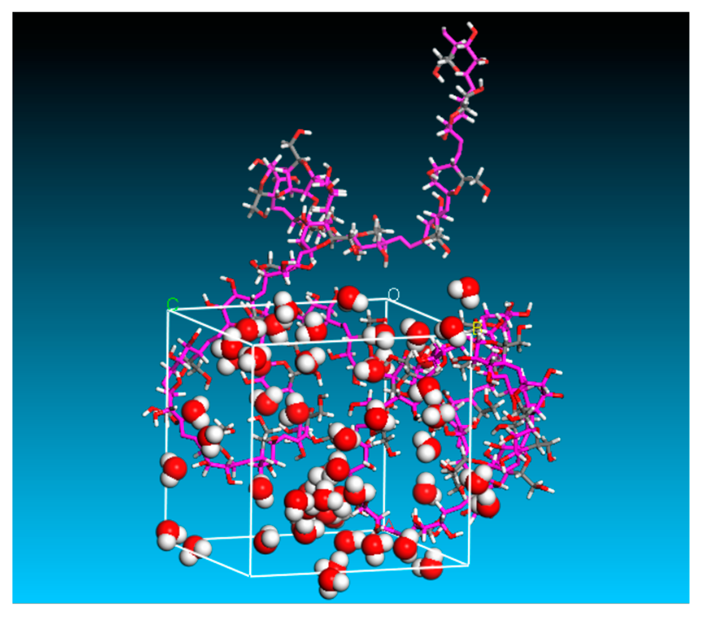
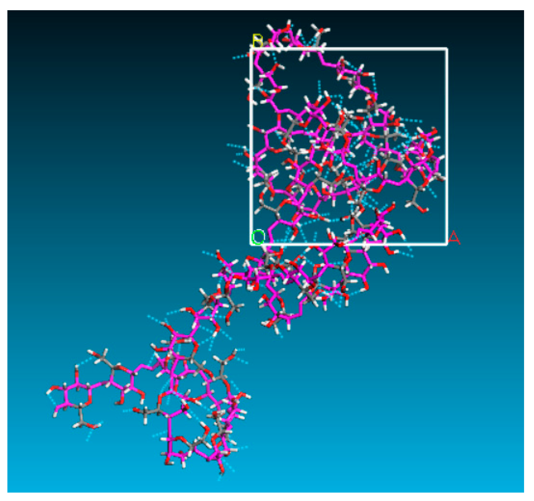
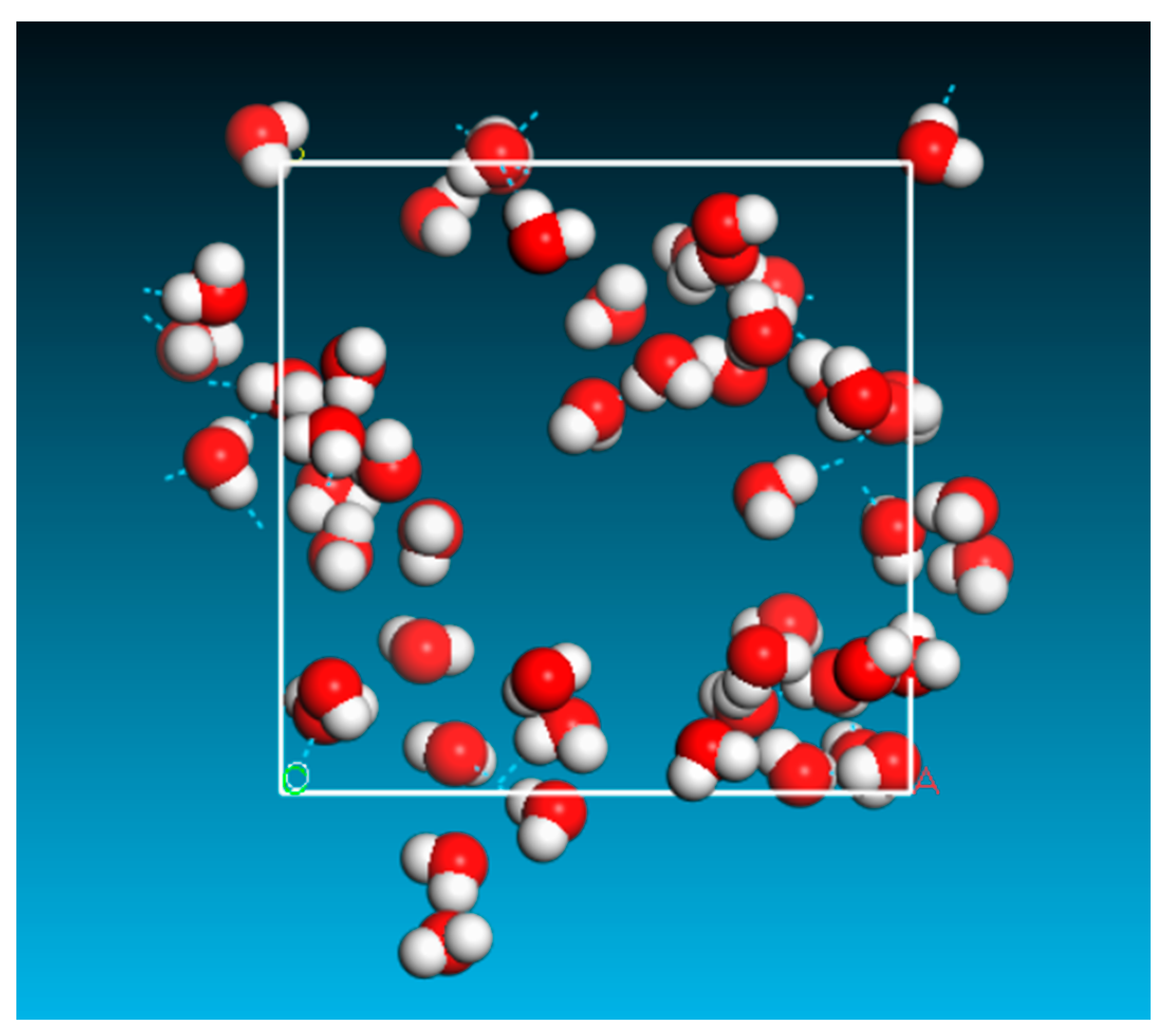
2.1. Model Establishment

The molecular dynamics simulation software in this paper is Materials Studio (2019, BIOVIA, San Diego, CA, USA), a PC-ready simulation software developed specifically for researchers in materials science. Before building the overall cellulose amorphous region-water model, the water molecule model and the cellulose chain need to be built separately. First, create a 3D document, click the Sketch Ring button on the sketch toolbar, and select Oxygen from the optional elements displayed. Click on the Adjust Hydrogen button to automatically add the correct number of hydrogen atoms to the model. Click on the Clean button to adjust the position of the model atoms so that bond lengths, bond angles, and torques are displayed appropriately. The structure of the cellulose chain is complex and can be drawn using the method for building amorphous polymers or by downloading the desired model from the materials project. Cellulose is composed of -D-glucopyranosyl (dehydrated glucose) with a simple molecular formula of (C₆H₁₀O₅)_n, where n is the degree of polymerization. The physicochemical properties of cellulose are not affected by changes in the degree of polymerization [35], so the degree of polymerization of cellulose chains established in this paper is 20. Calculations were performed with Amorphous cells to create a cellulose amorphous region-water model, which consists of 52 water molecules and a cellulose chain. The density of the model was set to 1.5 g/cm³ [36], and the final model was created with a box size of 20.5 × 20.5 × 20.5 ų. Figure 1 shows the cellulose amorphous region-water model with atoms in the model using the CPK color scheme, which was proposed and improved by Corey, Pauling, and Koltun, the designers of the CPK model. The gray, white, and red colors represent carbon, hydrogen, and oxygen atoms, respectively. To facilitate the distinction, cellulose chains are shown in stick mode, while water molecules are shown in ball and stick mode.

2.2. Dynamic Simulation

The model simulations in this paper follow the following steps:

• Create a molecular model structure of the studied system, including the simulation box size, the number of model molecules in the simulation box, and the specific atom types, as in Section 2.1.
• Perform initial geometry optimization of the initial molecular simulation model by the computational options in the Forcite module. The algorithm is chosen as the Smart algorithm [35], and the total number of iterations was 5000 steps. This step is to balance the free motion state of the molecules in the model so as to achieve energy minimization.
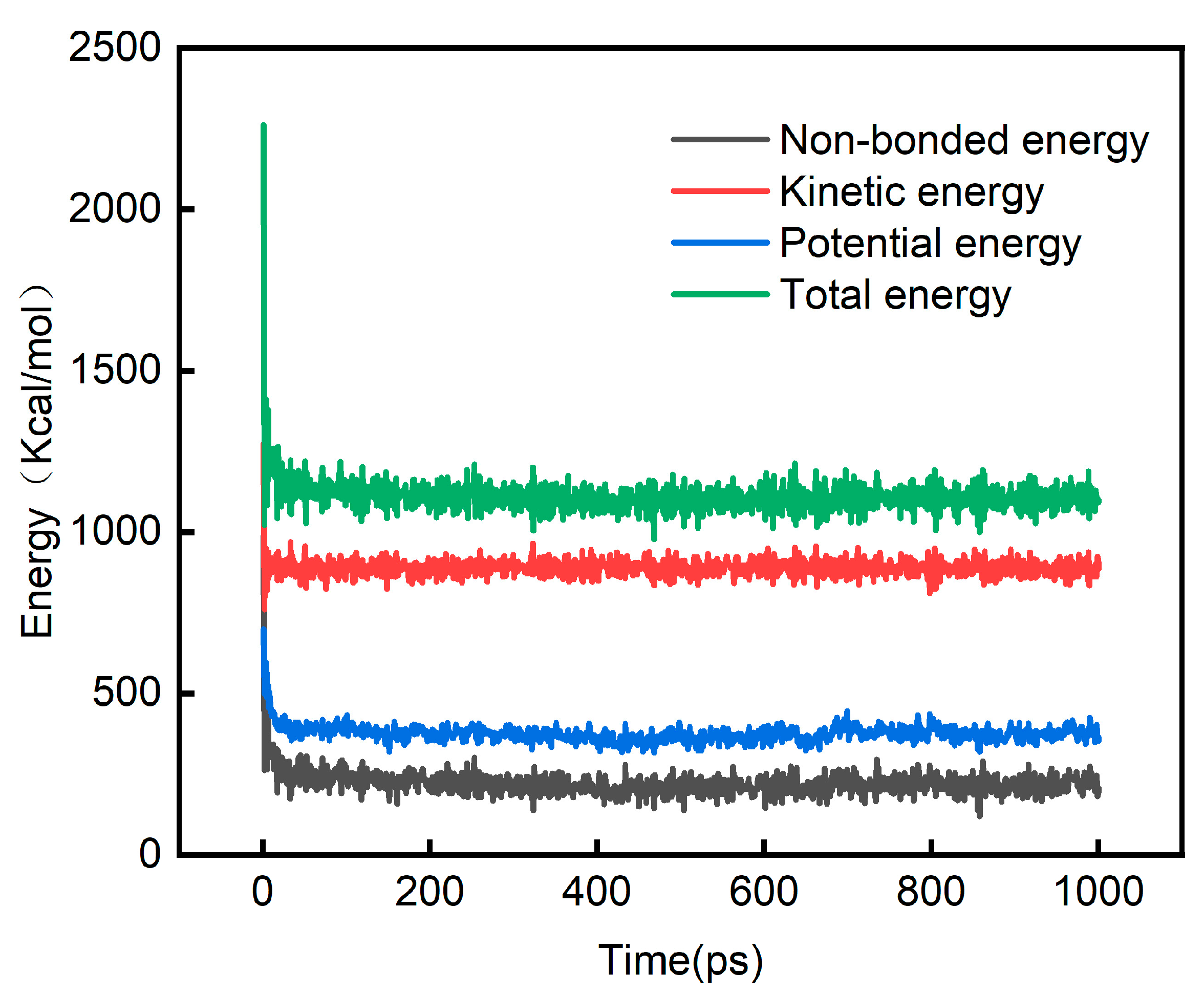
• The kinetic relaxation of the geometrically optimized model by the computational option in the Forcite module so that the model is in a lower energy stable state and the initial internal stress is reduced. The target temperature of the system is set to room temperature (25 °C), and the initial velocity is random. A total length of 1 ns is simulated under the macroscopic rule (NVT) system and the time step is set to 1 fs.
• After the system reached equilibrium and then entered into formal kinetic simulations for six sets (20 °C, 0 °C, −30 °C, −70 °C, −110 °C, and −150 °C). All six sets of simulations were performed at atmospheric pressure (0.1 MPa) and 1 ns under isothermal isobaric system synthesis (NPT). The pressure of the simulated experiments was controlled using the Berendsen method, chosen to be suitable for calculating the PCFF force field of natural polymer materials [30]. The electron summation was controlled by the Ewald method, and the van der Waals force calculation was controlled by the Atom-based method [37,38,39,40].

3. Results and Discussion

3.1. The Energy

3.1.1. System Energy

During each set of molecular dynamics simulations, fluctuations in each energy and temperature occur as the step size increases. The fluctuations of each energy of the system with the step size are shown in Figure 2.

The fluctuation value can determine whether the system is in equilibrium or not, and the system can be judged to be in equilibrium when the fluctuation range is between 5% and 10% [30]. The simulation accuracy can also be described by the energy convergence parameter [36], which is defined as follows:

$$\delta E=\frac{1}{N}\sum _{i=1}^N\left|\frac{E_i-E_0}{E_0}\right|$$

(1)

where $E_0$ denotes the initial energy of the simulated system, $E_i$ denotes the energy at which the molecular dynamics simulation proceeds to step $i$, and $N$ is the number of simulations. When $0.001<\delta E<0.003$, it means that the simulation results are reliable.

Taking the total energy change of the cellulose amorphous region-water molecule model at 20 °C as an example, $\delta E=0.001212$ is calculated, which proves that the energy of this simulated system converges. Therefore, it can be known that the system has stabilized and can be analyzed for interaction energy, etc.

3.1.2. Interaction Energy

Interaction energy reflects the interaction forces between different molecules and can explain the nature and laws of interactions between substances. The interaction forces between molecules are expressed in two aspects: on the one hand, the torsion and vibration of bond lengths and angles, and on the other hand, the non-bond interactions, including van der Waals and electrostatic interactions, etc. The total interaction energy, van der Waals interaction energy, and electrostatic interaction energy of matter can be calculated uniformly by Equation (2), and this calculation method was verified by Dihua Ouyang et al. [41].

$$E_{inter}=E_{total}-\left(E_a{+E}_b\right)$$

(2)

where $E_{inter}$ is the total interaction energy between substance $a$ and $b$, $\mathrm{k}\mathrm{c}\mathrm{a}\mathrm{l}/\mathrm{m}\mathrm{o}\mathrm{l}$; $E_{total}$ is the total potential energy of $a$ and $b$ mixed model, $\mathrm{k}\mathrm{c}\mathrm{a}\mathrm{l}/\mathrm{m}\mathrm{o}\mathrm{l}$; $E_a$ is the potential energy of substance $a$, $\mathrm{k}\mathrm{c}\mathrm{a}\mathrm{l}/\mathrm{m}\mathrm{o}\mathrm{l}$; $E_b$ is the potential energy of substance $b$, $\mathrm{k}\mathrm{c}\mathrm{a}\mathrm{l}/\mathrm{m}\mathrm{o}\mathrm{l}$.

The interaction energies of the cellulose amorphous region-water molecule model for different temperature effects during the simulation were obtained by compiling the program, as shown in

Table 1. Mean value of bond energy for different temperature models.

Temperature (°C)	20	0	−30	−70	−110	−150
$E_{total} (\mathrm{k}\mathrm{c}\mathrm{a}\mathrm{l}/\mathrm{m}\mathrm{o}\mathrm{l})$	1476	1417	1336	1158	1078	1002
$E_{cellulose} (\mathrm{k}\mathrm{c}\mathrm{a}\mathrm{l}/\mathrm{m}\mathrm{o}\mathrm{l})$	2170	2138	2075	1944	1893	1839
$E_{water} (\mathrm{k}\mathrm{c}\mathrm{a}\mathrm{l}/\mathrm{m}\mathrm{o}\mathrm{l})$	−93	−88	−89	−110	−136	−148
$E_{inter} (\mathrm{k}\mathrm{c}\mathrm{a}\mathrm{l}/\mathrm{m}\mathrm{o}\mathrm{l})$	−601	−633	−650	−676	−679	−689

.

The positive and negative values of interaction energy indicate that two substances repel or combine each other, and the larger the absolute value, the stronger the interaction [42]. It can be seen from Table 1 that the absolute value of the interaction energy between water molecules and cellulose chains increases as the temperature decreases. This shows that the model interacts stronger with decreasing temperature. The interaction energies of all six groups of models are negative, indicating that the water molecules and cellulose chains are attracted to each other, and the system can exist stably.

3.2. Model Volume and Density

The model formed by the cellulose amorphous region-water molecules is a square cubic box, and the size of this model can be expressed in terms of the length, width, and height of the box. The volume and density of the model change with temperature.

Table 2. The cell parameters of the cellulose amorphous region-water model at different temperatures.

Temperature (°C)	Cell Parameters (Å)
	The Length	The Width	The Height
20	20.88	20.88	20.88
0	20.82	20.82	20.82
−30	20.89	20.89	20.89
−70	20.78	20.78	20.78
−110	20.68	20.68	20.68
−150	20.65	20.65	20.65

shows the cellular parameters of the cellulose amorphous region-water molecule model at different temperatures.

At each temperature, the model was simulated in 1 ns steps, and the model parameters for each frame were summed and averaged to obtain the data in Table 2. From Table 2, it can be seen that the length, width, and height of the models decreased from 20.88 Å to 20.65 Å from 20 °C to −150 °C. Although there was a small increase in the length, width, and height of the models from 0 °C to −30 °C, the overall trend was decreasing. In order to observe the changes in the models at different temperatures more visually, the average values of the volume and density of each model were calculated, as shown in Figure 3.

Bodig and Jayne pointed out that the key factor affecting the tensile shear strength of wood is dense and that changes in density can also be used to characterize changes in mechanical properties [43]. The density increases, and the wood densification increases, further improving the mechanical properties. As can be seen in Figure 3, the density of the model tends to increase, and the volume tends to decrease as the temperature decreases. From 20 °C to −150 °C, the density of the model increased from 1.413 g/cm³ to 1.459 g/cm³, an increase of 3.26%. The volume decreases from 9098.866 ų to 8803.711 ų, a decrease of 3.24%. The changes in the model parameters can be verified against each other, and as the temperature decreases, the model interaction energy increases, the volume decreases, and the density increases, further affecting the mechanical properties.

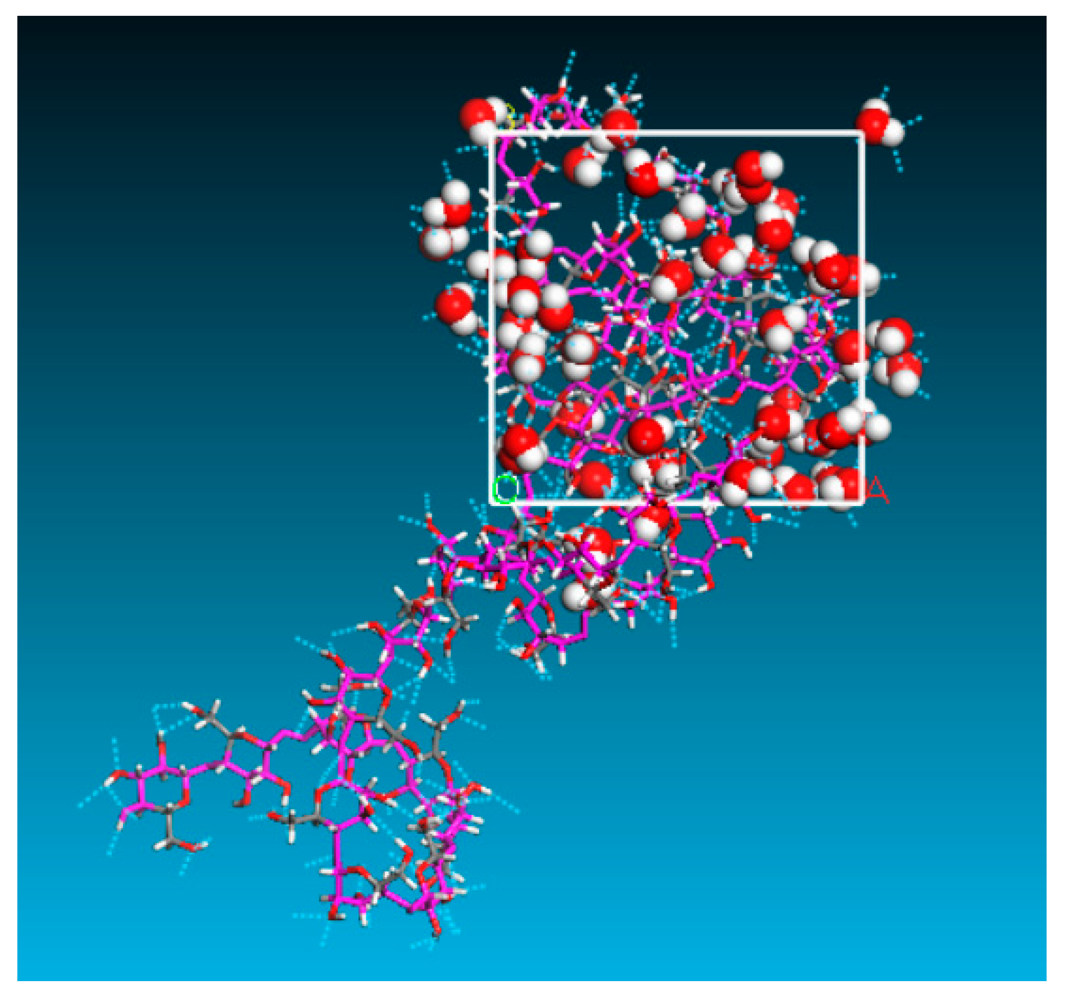
3.3. Hydrogen Bonding

Intermolecular hydrogen bonds are position-specific weak bonds and represent an important non-covalent interaction [44,45]. Hydrogen bonds form between electron-deficient hydrogen atoms and regions of high electron density, and the formation of intermolecular hydrogen bonds affects the chemical properties, charge distribution, and structure of donor and acceptor molecules [46,47]. Hydrogen bonds are essential structures in various fields of chemistry, physics and biochemistry, and they play an important role in the structure of biological proteins, DNA, and RNA [48]. As the temperature changes, the number of hydrogen bonds within the cellulose chain and between the cellulose chain and water also changes. The change in the number of hydrogen bonds plays an important role in the chemical and thermal stability and stability of the mechanical properties of cellulose molecules.

In our simulations, the geometric definition of hydrogen bonding for the simulations is that the distance between the hydrogen atom and the acceptor is less than 2 Å, and the angle formed by the donor, hydrogen atom, and acceptor is greater than 110°. This hydrogen bonding parameter is the same as the setting conditions for hydrogen bonding within cellulose determined by Nishiyama’s experiment. Figure 4, Figure 5 and Figure 6 represent the hydrogen bonding distribution within the cellulose amorphous region-water molecule model, cellulose amorphous region model, and water molecule model, using the kinetic model at 20 °C as an example.

The calculated hydrogen bonding module in Material Studio software was used to analyze the hydrogen bonds, and Perl scripts were used to count the number of hydrogen bonds.

Table 3. Number of hydrogen bonds for different temperature models.

Temperature (°C)	20	0	−30	−70	−110	−150
$H_{total}$	229.20	232.01	235.22	244.80	244.64	251.59
$H_{cellulose}$	87.00	83.85	86.37	89.21	89.60	85.89
$H_{water}$	32.69	30.23	28.62	32.96	38.66	34.99
$H_{inter}$	109.51	117.94	120.23	122.63	116.38	130.71

shows the distribution of the number of hydrogen bonds in the cellulose amorphous region-water molecule model at different temperatures. $H_{total}$ indicates the total number of hydrogen bonds inside the model, $H_{cellulose}$ indicates the number of hydrogen bonds within the cellulose chains, $H_{water}$ indicates the number of hydrogen bonds between water molecules, and $H_{inter}$ indicates the number of hydrogen bonds between water molecules and cellulose chains.

As can be seen from the above table, the number of total hydrogen bonds and the number of hydrogen bonds between water molecule–cellulose chains increased for each model as the temperature decreased. Although there were also small changes in the hydrogen bonds within the cellulose chains and the hydrogen bonds within the water molecules, the increase in the total number of hydrogen bonds in each model mainly came from the increase in the number of hydrogen bonds between the water molecule–cellulose chains. In terms of the number of hydrogen bonds, the number of hydrogen bonds between water molecule–cellulose chains accounted for nearly half of the total number of hydrogen bonds in the model and was far greater than the number of hydrogen bonds within the cellulose chains. This fully indicates that the hydrogen bonds between cellulose chains play an important role in maintaining the mechanical properties and chemical stability of cellulose materials. The decrease in temperature weakens the activity of the cellulose molecular, and the increase in the number of hydrogen bonds will inevitably improve the mechanical properties and chemical stability of the cellulose materials.

3.4. Mechanical Properties

Molecular dynamics simulations allow the calculation of the static mechanical properties of polymers and thus indirectly characterize the compatibility of the blended system phases and the macroscopic mechanical properties. For an equilibrium blend system, the mechanical properties parameters of the system can be obtained by applying minor stress and counting the strain information of the material during the kinetic simulation [49]. The material stress–strain relationship satisfies Hooke’s law in Equation (3).

$${\sigma }_i={\mathrm{C}}_{ij}{\epsilon }_j$$

(3)

where ${\mathrm{C}}_{ij}$ is the material elastic matrix coefficient, ${\sigma }_i$ and ${\epsilon }_j$ are the stress and strain vectors, respectively, and Equation (3) can be expanded into Equation (4).

$$\left[\begin{array}{c}{\sigma }_x\\ {\sigma }_y\\ {\sigma }_z\\ {\sigma }_{yz}\\ {\sigma }_{zx}\\ {\sigma }_{xy}\end{array}\right]=\left[\begin{array}{cccccc}{\mathrm{C}}_{11}& {\mathrm{C}}_{12}& {\mathrm{C}}_{13}& {\mathrm{C}}_{14}& {\mathrm{C}}_{15}& {\mathrm{C}}_{16}\\ {\mathrm{C}}_{21}& {\mathrm{C}}_{22}& {\mathrm{C}}_{23}& {\mathrm{C}}_{24}& {\mathrm{C}}_{25}& {\mathrm{C}}_{26}\\ {\mathrm{C}}_{31}& {\mathrm{C}}_{32}& {\mathrm{C}}_{33}& {\mathrm{C}}_{34}& {\mathrm{C}}_{35}& {\mathrm{C}}_{36}\\ {\mathrm{C}}_{41}& {\mathrm{C}}_{42}& {\mathrm{C}}_{43}& {\mathrm{C}}_{44}& {\mathrm{C}}_{45}& {\mathrm{C}}_{46}\\ {\mathrm{C}}_{51}& {\mathrm{C}}_{52}& {\mathrm{C}}_{53}& {\mathrm{C}}_{54}& {\mathrm{C}}_{55}& {\mathrm{C}}_{56}\\ {\mathrm{C}}_{61}& {\mathrm{C}}_{62}& {\mathrm{C}}_{63}& {\mathrm{C}}_{64}& {\mathrm{C}}_{65}& {\mathrm{C}}_{66}\end{array}\right]\left[\begin{array}{c}{\epsilon }_x\\ {\epsilon }_y\\ {\epsilon }_z\\ {\epsilon }_{yz}\\ {\epsilon }_{zx}\\ {\epsilon }_{xy}\end{array}\right]$$

(4)

The stress component can be calculated by Equation (5):

$${\sigma }_{ij}=-\frac{1}{V}\sum _k{m}^k\left(u_i^k{u}_j^k\right)+\frac{1}{2}\sum _{i\ne k}\left(r_i^{kl}\right)f_j^{lk}$$

(5)

The mass and velocity of the kth particle are $m^k$ and $u^k$, $r^{kl}$ denotes the relative distance between particle $k$ and particle $i$, and $f^{lk}$ denotes the interaction force between particle $k$ and particle $i$.

The elastic constant coefficients $\lambda$ and $\mu$ can be calculated by Equations (6) and (7) based on the elasticity coefficient matrix.

$$\lambda =\frac{1}{6}({\mathrm{C}}_{12}+{\mathrm{C}}_{13}+{\mathrm{C}}_{21}+{\mathrm{C}}_{23}+{\mathrm{C}}_{31}+{\mathrm{C}}_{32})\approx \frac{1}{3}({\mathrm{C}}_{12}+{\mathrm{C}}_{23}+{\mathrm{C}}_{13})$$

(6)

$$\mu =\frac{1}{3}({\mathrm{C}}_{44}+{\mathrm{C}}_{55}+{\mathrm{C}}_{66})$$

(7)

The Young’s modulus $E$, bulk modulus $K$, shear modulus $G$, and Poisson’s ratio $\gamma$ of the system can be calculated.

$$E=\frac{\mu (3\lambda +2\mu )}{\lambda +\mu }$$

(8)

$$G=\mu$$

(9)

$$\gamma =\frac{\lambda }{2(\lambda +\mu )}$$

(10)

$$K=\lambda +\frac{2}{3\mu }$$

(11)

Young’s modulus ($E$) refers to the ratio of the force required to stretch per unit length along the central axis of the material to the cross-section of the material. It is used to describe the strength of the material, with a numerical magnitude proportional to the rigid strength of the material. In the linear tensile region of polymers, Young’s modulus is positively related to the tensile strength of the material. The bulk modulus ($K$) is used to characterize the incompressible properties of the material. The shear modulus ($G$) is the ratio of the shear stress to the shear strain, which characterizes the ease of shear strain of the material. The $K/G$ value is the size of the deformation of the material under the same external stress, which is used to characterize the ductility and toughness of the material. The variation of the mechanical parameters of each model at different temperatures was calculated by molecular dynamics simulation, as shown in

Table 4. Mechanical parameters for different temperature models.

Temperature (°C)	20	0	−30	−70	−110	−150
${\mathrm{C}}_{12}$	8.29	8.01	10.31	10.30	9.73	11.00
${\mathrm{C}}_{13}$	8.38	7.83	9.82	10.54	12.58	11.18
${\mathrm{C}}_{23}$	7.49	8.02	9.72	11.71	11.64	11.62
${\mathrm{C}}_{44}$	4.07	5.11	8.42	5.28	6.17	9.06
${\mathrm{C}}_{55}$	1.97	4.29	7.15	6.32	6.24	7.26
${\mathrm{C}}_{66}$	5.61	3.38	8.22	6.79	7.60	7.32
$\lambda$	8.05	7.95	9.95	10.85	11.32	11.27
$\mu =G$	3.88	4.26	7.93	6.13	6.67	7.88
$E$	10.39	11.30	20.27	16.18	17.54	20.40
$K$	8.23	8.11	10.04	10.96	11.42	11.35
$K/G$	2.12	1.90	1.27	1.79	1.71	1.44

.

The mechanical properties of wood tend to increase when it is placed below room temperature. When wood is heated, its mechanical properties decrease [6,50], and similar results were observed in the present study. As the temperature decreases, the values of G, E, and K increase, and the resistance to deformation, incompressible properties, and the difficulty of material shear strain is enhanced. When the temperature decreases to −150 °C, K/G decreases to the minimum value, indicating that the ductility and toughness gradually decrease at this time. Overall, it is shown that the temperature decrease is beneficial in enhancing the mechanical properties of the amorphous cellulose region and increases the stiffness of the material. However, the ductility and plasticity decrease when the temperature is too low. In addition, the increase in BS and MOE strength of wood at temperatures below the freezing temperature may explain the results of our study. Schmidt and Pomeroy [51] suggested that the increase in wood stiffness at lower temperatures may be due to the formation of ice crystals in the wood cavities.

4. Conclusions

In this paper, the effect of low temperature on the properties of the amorphous region of lignocellulose, the main component of wood, was investigated. Molecular dynamics studies were carried out in NPT combinations at 20 °C, 0 °C, −30 °C, −70 °C, −110 °C, and −150 °C. The changes in the microstructure of the water molecule–cellulose amorphous region model were analyzed, and the mechanical properties were calculated by the trends of energy, volume, density, and hydrogen bonding changes in the model. The data from microscopic simulations explain and illustrate how the main components of wood change when it is in a low-temperature environment. It is of great theoretical significance and practical value to provide a theoretical reference for expanding the application of wood in low-temperature environments. The conclusions obtained are as follows:

• The absolute value of the interaction energy between water molecules and cellulose chains increases as the temperature decreases. It indicates that the interaction between water molecules and cellulose amorphous region is stronger by decreasing the temperature. The interaction energies of the six groups of models at different temperatures are all negative, indicating that water molecules and cellulose chains are attracted to each other, and the system can exist stably.
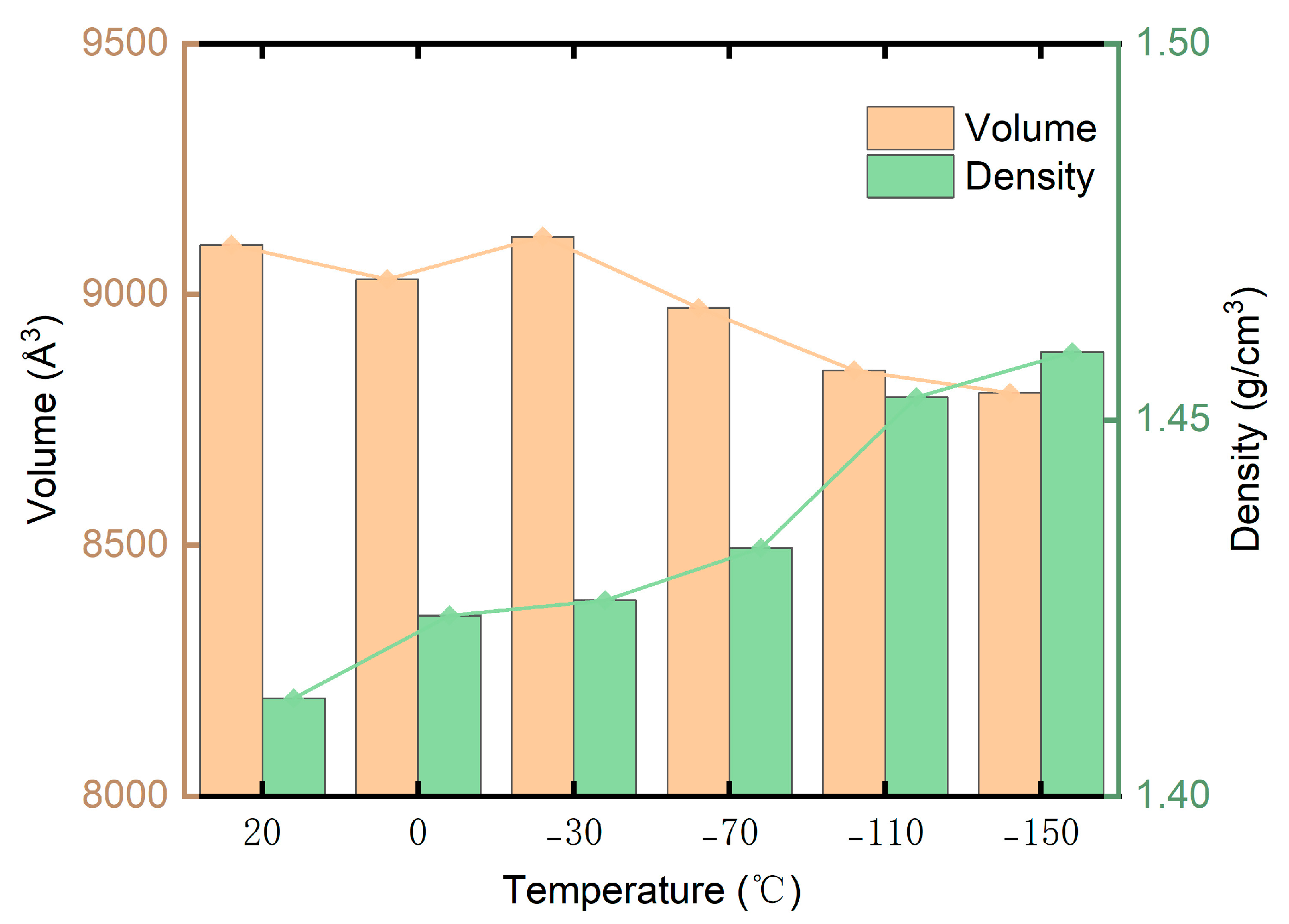
• From 20 °C to −150 °C, the model density increased from 1.413 g/cm³ to 1.459 g/cm³, an increase of 3.26%. The volume decreases from 9098.866 ų to 8803.711 ų, a decrease of 3.24%. The internal structure of the model is influenced by the temperature, and the changes in the model parameters can be verified with the interaction energy with each other. As the temperature decreases, the model interaction energy increases, the volume decreases, and the density increases.
• The decrease in temperature makes cellulose molecular activity weaker. The total number of hydrogen bonds and the number of hydrogen bonds between water molecule–cellulose chains for each model increased with decreasing temperature. The new interchain hydrogen bonds enhanced the restraining effect on the arrangement of cellulose molecular chains. The values of G, E, and K increased with decreasing temperature, and K/G decreased with decreasing temperature. The low-temperature treatment increased the stiffness and reduced the toughness of the wood. The changes in mechanical properties were characterized by the number of hydrogen bonds to each other, and the increase in the number of hydrogen bonds will inevitably increase the mechanical properties and chemical stability of the cellulose material.

References

1. Esteves, B.; Pereira, H. Wood modification by heat treatment: A review. BioResources 2009, 4, 370–404. [Google Scholar] [CrossRef]
2. Ma, X.; Zhang, F.; Wei, L. Effect of wood charcoal contents on the adsorption property, structure, and morphology of mesoporous activated carbon fibers derived from wood liquefaction process. J. Mater. Sci. 2014, 50, 1908–1914. [Google Scholar] [CrossRef]
3. Wei, L.; Liang, S.; McDonald, A.G. Thermophysical properties and biodegradation behavior of green composites made from polyhydroxybutyrate and potato peel waste fermentation residue. Ind. Crops Prod. 2015, 69, 91–103. [Google Scholar] [CrossRef]
4. Wei, L.; McDonald, A.G.; Stark, N.M. Grafting of bacterial polyhydroxybutyrate (PHB) onto cellulose via in-situ reactive extrusion with dicumyl peroxide. Biomacromolecules 2015, 16, 1040–1049. [Google Scholar] [CrossRef]
5. Carlmark, A.; Larsson, E.; Malmström, E. Grafting of cellulose by ring-opening polymerization—A review. Eur. Polym. J. 2012, 48, 1646–1659. [Google Scholar] [CrossRef] [Green Version]
6. Green, D.W.; Evans, J.W.; Logan, J.D.; Nelson, W.J. Adjusting modulus of elasticity of lumber for changes in temperature. For. Prod. J. 1999, 49, 82–94. [Google Scholar]
7. Lv, J.X.; Lin, Z.Y.; Jiang, J.L. Influence of different drying methods on the infiltration properties of wood from fir plantations. For. Sci. 2006, 4, 85–90. [Google Scholar]
8. Schaffer, E.L. Effect of pyrolytic temperatures on longitudinal strength of dry Douglas-fir. J. Test. Eval. 1973, 1, 319–329. [Google Scholar]
9. Moraes, P.D.; Rogaume, Y.; Bocquet, J.F. Influence of temperature on the embedding strength. Holz Roh-Werkst 2005, 63, 297–302. [Google Scholar] [CrossRef]
10. Adewopo, J.B.; Patterson, D.W. Effects of heat treatment on the mechanical properties of Loblolly Pine, Sweetgum, and Red Oak. For. Prod. J. 2011, 61, 526–535. [Google Scholar] [CrossRef]
11. Zhou, J.H.; Hu, C.S.; Hu, S.F. Effects of temperature on the bending performance of wood-based panels. BioResources 2012, 7, 3597–3606. [Google Scholar]
12. Kubojima, Y.; Okano, T.; Ohta, M. Bending strength and toughness of heat-treated wood. J. Wood Sci. 2000, 46, 8–15. [Google Scholar] [CrossRef]
13. Moraes, P.; Rogaume, Y.; Triboulot, P. Influence of temperature on the modulus of elasticity (MOE) of Pinus sylvestris L. Holzforschung 2004, 58, 143–147. [Google Scholar] [CrossRef]
14. Windeisen, E.; Bchle, H.; Zimmer, B. Relations between chemical changes and mechanical properties of thermally treated wood. Holzforschung 2009, 63, 773–778. [Google Scholar] [CrossRef]
15. Awoyemi, L.; Jones, I.P. Anatomical explanations for the changes in properties of western red cedar (Thujaplicata) wood during heat treatment. Wood Sci. Technol. 2011, 45, 261–267. [Google Scholar] [CrossRef]
16. Kamody, D.J. Using deep cryogenic to advantage. Adv. Mater. Process. 1998, 154, 215–218. [Google Scholar]
17. Yi, X.; Chen, D. Research progress on deep cooling treatment of composite materials. Met. Heat Treat. 2012, 37, 73–76. [Google Scholar]
18. Owaku, S. Cryogenic treatment. Heat. Treat. 1981, 21, 44–48. [Google Scholar]
19. Kalia, S. Cryogenic processing: A study of materials at low temperatures. J. Low Temp. Phys. 2010, 158, 934–945. [Google Scholar] [CrossRef]
20. Yamada, T. Temperature Dependency of Physical Properties of Wood at Low Temperature; Kyoto University Research Information Repository: Kyoto, Japan, 1971. [Google Scholar]
21. Berner, D.; Gerwick, B.C.; Polivka, M. Static and cyclic behavior of structural lightweight concrete at cryogenic temperatures. In Temperature Effects on Concrete ASTM International; Springer: Tokyo, Japan, 1985. [Google Scholar]
22. DeGeer, D.; Bach, L. Machine Stress Grading of Lumber at Low Temperatures; Alberta Research Council: Edmonton, AB, Canada, 1995. [Google Scholar]
23. Xu, H.D.; Wang, Y.T.; Wang, L.H.; Wang, X.P. A review on ice formation and propagation in wood cells at subzero temperatures. J. Nanjing For. Univ. 2017, 41, 169–174. [Google Scholar]
24. Li, Z.; Jiang, J.L.; Lu, J.X. Moisture-dependent orthotropic viscoelastic properties of Chinese fir wood in low temperature environment. J. Wood Sci. 2018, 64, 515–525. [Google Scholar] [CrossRef] [Green Version]
25. Ozkan, O.E. Effect of Freezing Temperature on Impact Bending Strength and Shore-D Hardness of Some Wood Species. BioResources 2022, 17, 6123–6130. [Google Scholar] [CrossRef]
26. Paschalina, T.; Vasiliki, K. Chemical characterization of Wood and Bark biomass of the invasive species of Tree-of-heaven (Ailanthus altissima (Mill.) Swingle), focusing on its chemical composition horizontal variability assessment. Wood Mater. Sci. Eng. 2022, 17, 469–477. [Google Scholar]
27. Jiang, X.W.; Wang, W.; Guo, Y.Y.; Dai, M. Effect of pressurized hydrothermal treatment on the properties of cellulose amorphous region based on molecular dynamics simulation. Forestry 2023, 14, 314. [Google Scholar] [CrossRef]
28. Khazraji, A.C.; Robert, S. Interaction effects between cellulose and water in nanocrystalline and amorphous regions: A novel approach using molecular modeling. J. Nanomater. 2013, 2013, 44. [Google Scholar] [CrossRef] [Green Version]
29. Hou, T.J.; Zhang, W.; Xu, X.J. Binding affinities for a series of selective inhibitors of gelatinase-A using molecular dynamics with a linear interaction energy approach. J. Phys. Chem. B 2005, 105, 5304–5315. [Google Scholar] [CrossRef]
30. Wang, W.; Ma, W.; Wu, M.; Sun, L. Effect of Water Molecules at Different Temperatures on Properties of Cellulose Based on Molecular Dynamics Simulation. BioResources 2020, 17, 269–280. [Google Scholar] [CrossRef]
31. Karplus, M.; McCammon, J.A. Molecular dynamics simulations of biomolecules. Nat. Struct. Biol. 2002, 9, 646–652. [Google Scholar] [CrossRef]
32. Steinhauser, M.O.; Hiermaier, S. A review of computational methods in materials science: Examples from shock-wave and polymer physics. Int. J. Mol. Sci. 2009, 10, 5135–5216. [Google Scholar] [CrossRef] [Green Version]
33. Hollingsworth, S.A.; Dror, R.O. Molecular dynamics simulation for all. Neuron 2018, 99, 1129–1143. [Google Scholar] [CrossRef] [Green Version]
34. Liu, C.B.; Sun, Z. Molecular dynamics simulation of phase transition process in nematic liquid crystal materials. Mech. Sci. Technol. 2023, 33, 1–9. [Google Scholar]
35. Mazeau, K.; Heux, L. Molecular dynamics simulations of bulk native crystalline and amorphous structures of cellulose. J. Phys. Chem. B 2003, 107, 2394–2403. [Google Scholar] [CrossRef]
36. Allen, M.P.; Tildesley, D.J. Computer Simulation of Liquids; Clarendon Press: Oxford, UK, 2017. [Google Scholar]
37. Ewald, P. Evaluation of optical and electrostatic lattice potentials. Ann. Phys. 1921, 64, 253–287. [Google Scholar] [CrossRef] [Green Version]
38. Andersen, H.C. Molecular dynamics simulations at constant pressure and/or temperature. J. Chem. Phys. 1980, 72, 2384–2393. [Google Scholar] [CrossRef] [Green Version]
39. Andrea, T.A.; Swope, W.C.; Andersen, H.C. The role of long ranged forces in determining the structure and properties of liquid water. J. Chem. Phys. 1983, 79, 4576–4584. [Google Scholar] [CrossRef]
40. Berendsen, H.J.; Postma, J.V.; Van Gunsteren, W.F.; DiNola, A.; Haak, J.R. Molecular dynamics with coupling to an external bath. J. Chem. Phys. 1984, 81, 3684–3690. [Google Scholar] [CrossRef] [Green Version]
41. Ouyang, D.; Zhang, L.; Mao, R.; Qin, X.; Pang, W. Application Process of Coating Agent and the Coating Effect Evaluation Based on Molecular Dynamics. Langmuir 2023, 39, 3411–3419. [Google Scholar] [CrossRef]
42. Hanus, J.; Mazeau, K. The xyloglucan-cellulose assembly at the atomic scale. Biopolymers 2006, 82, 59–73. [Google Scholar] [CrossRef]
43. Bodig, J.; Jayne, B.A. Mechanic of Wood and Wood Composites; Van Nostrand Reinhold: New York, NY, USA, 1982. [Google Scholar]
44. Zhang, Y.; Duan, Y.; Liu, J. The effect of intermolecular hydrogen bonding on the polyaniline water complex. J. Cluster Sci. 2017, 28, 1071. [Google Scholar] [CrossRef] [Green Version]
45. Zheng, Y.; Deng, G.; Guo, R. A DFT-based study of the hydrogen-bonding interactions between myricetin and ethanol/water. J. Mol. Model. 2019, 25, 67. [Google Scholar] [CrossRef]
46. Mishra, S.; Suryaprakash, N. Intramolecular hydrogen bonding involving organic fluorine: NMR investigations corroborated by DFT-based theoretical calculations. Molecules 2017, 22, 423. [Google Scholar] [CrossRef] [PubMed] [Green Version]
47. Juan, Y.; An, Y.L. Theoretical study of hydrogen bonding excited states of fluorenone with formaldehyde. Comput. Theor. Chem. 2016, 1101, 62. [Google Scholar]
48. Yang, J.; Li, A.Y. Hydrogen bond strengthening between o-nitroaniline and formaldehyde in electronic excited states:A theoretical study. Spectrochim. Acta A 2018, 199, 194. [Google Scholar] [CrossRef]
49. Du, D.Y.; Tang, C.; Zhang, J.W. Effects of hydrogen sulfide on the mechanical and thermal properties of cellulose insulating paper: A molecular dynamics simulation. Mater. Chem. Phys. 2020, 240, 122153. [Google Scholar] [CrossRef]
50. Ozer, I. Some Mechanical Properties of Frozen Juvenile and Mature Wood of Pinus Nigra Var pallasiana Aral. and Pinus brutia Ten; Institute of Natural Sciences, Istanbul University: Istanbul, Turkey, 2002; Volume 75. [Google Scholar]
51. Schmidt, R.A.; Pomeroy, J.W. Bending of a conifer branch at subfreezing temperatures: Implications for snow interception. Can. J. For. Res. 1990, 20, 1250–1253. [Google Scholar] [CrossRef]
Figure 1. The cellulose amorphous region-water molecule model.
Forests 14 01208 g001
Figure 2. Energy-time variation chart.
Forests 14 01208 g002
Figure 3. The density and volume of the cellulose amorphous region-water model at different temperatures.
Forests 14 01208 g003
Figure 4. Hydrogen bonding distribution of cellulose amorphous region-water molecule model.
Forests 14 01208 g004
Figure 5. Hydrogen bonding distribution in the amorphous region of cellulose.
Forests 14 01208 g005
Figure 6. Hydrogen bonding distribution within the water molecule model.
Forests 14 01208 g006