Disturbance-Dependent Variation in Functional Redundancy Drives the Species Versus Functional Diversity Relationship across Spatial Scales and Vegetation Layers

Abstract

Since species’ traits are closely linked to ecosystem functioning, the species versus functional diversity relationship (the SD–FD relationship) is considered a valuable indicator of ecosystem health. However, the extent to which the SD–FD relationship varies among disturbed versus undisturbed subtropical forests and whether the conclusion depends on the spatial scale of the observation or vegetation layer remains unclear. In this study, using plots of 100 m², 400 m² and 2000 m², we gathered species and functional diversity data for woody and non-woody vegetation from replicate sites of undisturbed mature forests versus disturbed shrubland and plantations from subtropical China. Our analyses indicated that the species richness versus functional richness relationship, as well as the species evenness versus functional evenness relationship, varies markedly among disturbed versus undisturbed forests and woody versus non-woody layers. Scale-dependent variations in the SD–FD relationship were evident mainly in the woody layers or evenness component. Additional analyses revealed that disturbance-dependent variation in the community-level functional redundancy and species-level functional uniqueness can partly explain the observed variation in the SD–FD relationships. Overall, our study demonstrated that the SD–FD relationships are positive, but the relationship’s slope varies with contexts, partly due to variations in community-level functional redundancy and species-level functional uniqueness.

1. Introduction

One of the central goals of ecosystem management is to maintain healthy ecosystems that are rich in species and well-functioning. To achieve that goal, practitioners have traditionally emphasized conserving the number of species, assuming that the higher the number of species, the healthier the ecosystem [1,2]. While the positive association between species diversity and ecosystem functioning confirms such assumptions in relatively simple and experimental systems [3,4], validating the idea in relatively complex and natural systems remains challenging [5]. In such a context, examining the relationship between species and functional diversity (hereafter referred to as the SD–FD relationship) can be handy, as species’ traits usually govern ecosystem functioning [2]. Hence, understanding how the SD–FD relationship varies among disturbed versus undisturbed habitats can also help assess the relative health of disturbed habitats [5].

In the past, such an approach has been applied to grasslands, riparian systems, arid-land and countryside plant communities, yielding positive to negative to non-significant SD–FD relationships [5,6,7,8,9,10,11]. However, those studies employed different plot sizes and focused on either woody or non-woody vegetation, or sometimes both. It remains unclear whether the varying results regarding disturbance-dependent variation in the SD–FD relationship depend on the spatial scale of observation (cf. plot size) or the vegetation layer. Furthermore, little is known about the extent to which the SD–FD relationship varies among disturbed versus undisturbed habitats in subtropical forests, which are rich in species, exhibit distinct woody and non-woody vegetation layers, and experience unique anthropogenic disturbances [12,13].

Most research suggests that community-level functional redundancy (the number of species in a community that supports a given function or multiple functions) and species-level functional uniqueness (how important is a focal species in supporting a given function or multiple functions) are important drivers of the SD–FD relationship [7,8,9,14]. Increasing the number of species may lead to a proportionately increased functional diversity (i.e., a strongly positive relationship) if communities are composed of diverse functional traits (moderate community-level redundancy) and species-level functional uniqueness is, on average, high. By contrast, increasing species richness may not increase functional diversity proportionately (i.e., weakly positive or no significant relationship) if community members possess highly similar functional traits (i.e., high to moderate community-level redundancy) and moderate to low species-level functional uniqueness. However, because species and functional diversity and redundancy patterns vary with the nature of disturbance (type, intensity, frequency, seasonality, or time since disturbance), the SD–FD relationships vary accordingly [5,6,7,8,9,10].

In the subtropical forest, clear-cutting followed by monospecific plantation raising or converting the relatively intact mature forests into shrubland via selective cutting for fuelwood often yields different diversity patterns [12,13]. For instance, plantations are typically poor in species and functional diversity, while undisturbed mature forests and moderately disturbed shrublands are biodiversity-rich [15]. Resource acquisition strategies usually dominate those plantations (e.g., species with high leaf area, specific leaf area, leaf nitrogen and phosphorus concentrations); in contrast, mature forests and moderately-disturbed shrublands are dominated by plants having a resource conservation strategy (high leaf thickness, leaf dry matter content and C:N) [12]. So, plantation forests might have high community-level functional redundancy and low species-level functional uniqueness (due to planting a few species), and disturbed shrublands should have moderate redundancy and moderate species-level functional uniqueness (due to post-disturbance natural colonization of species). In contrast, undisturbed mature forests should have moderate redundancy and high functional uniqueness at the species level (due to competition-mediated community assembly). Consequently, we can hypothesize that the SD–FD relationship in plantations should be characterized by a low intercept and flat slope. At the same time, those in shrublands and mature forests should have high intercepts and relatively steeper slopes (Figure 1).

However, processes shaping species and functional diversity or redundancy patterns, such as habitat filtering and biotic competition, often vary with the observation window [16,17,18]. So, the spatial scale of observation could be another crucial factor here [19]. The concept of the species-area relationship also suggests that species and functional diversity usually increase with an increasing area [20,21]. Functional redundancy patterns are thus likely to be idiosyncratic at a small scale but may stabilize at a large scale due to the addition of (functionally) similar or unique species. In a disturbed habitat, the added species with increasing plot size/area are likely to be functionally similar, while those in undisturbed habitats are likely to be rare and functionally unique. So, increasing plot size in a disturbed habitat may result in an overall increase in community-level functional redundancy and low species-level functional uniqueness, while it may reduce functional redundancy and increase the overall value of species-level functional uniqueness in undisturbed habitats. The SD–FD relationships for disturbed versus undisturbed habitats may thus also vary with spatial scale. More specifically, we expect relatively steeper slopes for SD–FD relationships at small to moderate scales than on a large scale (Figure 1).

Another crucial aspect concerning the SD–FD relationship is the vegetation layers. Overstory woody and understory non-woody species have different resource requirements and experience disturbance differently [22]. While clear-cutting followed by plantation raising removes both overstory and understory vegetation, selective cutting for firewoods (the case for shrubland) removes overstory vegetation only [15]. In addition, woody vegetation in the overstory usually shows aggregation at a broader scale, while non-woody vegetation in the understory shows aggregation at a smaller scale. So, functional diversity patterns and potential variations in the SD–FD relationships among disturbed and undisturbed forests may further vary among vegetation layers (Figure 1).

Meanwhile, species and functional diversity have multiple facets, including richness and evenness [23,24]. So, the critical question is: do the hypothesized disturbance, spatial scale, and vegetation-layer-dependent variation in the SD–FD relationship (discussed above and highlighted in Figure 1) remain consistent across different indices of diversity such as species richness versus functional richness (FRic), species evenness versus functional evenness (FEve), and species diversity (Shannon’s diversity) versus functional diversity (Rao’s Q)? We argue that all three relationships, namely species richness versus functional richness (FRic), species evenness versus functional evenness (FEve), and species diversity (Shannon’s diversity) versus functional diversity (Rao’s Q), would generally vary with disturbance and vegetation layers. However, the magnitude of variation might vary among indices for several reasons. For instance, when the disturbance directly removes entire vegetation, as is the case for clear-cutting followed by plantation raising, disturbance effects are often felt on richness. But when disturbance removes vegetation selectively, as is the case for shrubland, disturbance effects are first felt on changes in species abundance distributions, in turn on evenness. The species versus functional richness relationship is thus expected to vary remarkably among mature forests versus plantations, and the species evenness versus functional evenness relationship is expected to vary among mature forests versus shrublands versus plantations. We expect the above pattern to be consistent across scales.

The Tiantong National Forest Park in eastern China is an ideal forest for the current study because (i) it represents subtropical evergreen broad-leaf forests, (ii) it includes areas of intact mature forest and areas of anthropogenically disturbed shrublands and plantations, and (iii) the disturbance and management history of the forest are well documented [25]. While past research from this forest has looked into the community assembly processes and spatial vegetation patterns, there is still a lack of studies examining community- or species-level functional redundancy/uniqueness and the resultant variations in species and functional diversity relationships. So, in the present study, we gathered data on species and functional diversity and asked three questions:

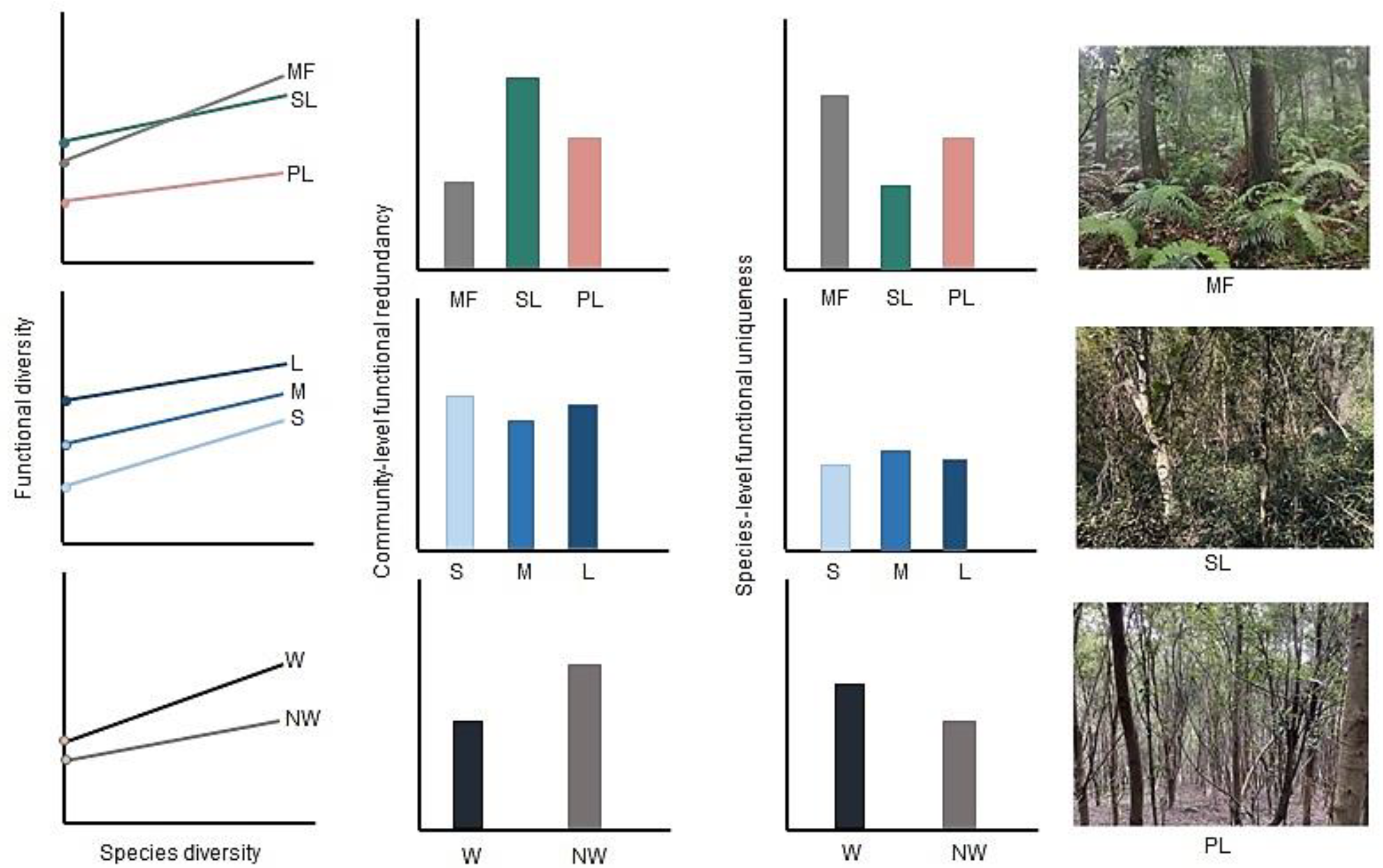
• Do SD–FD relationships (i.e., relationships between species richness and functional richness, species evenness and functional evenness, and Shannon’s species diversity and Rao’s functional diversity) vary among intact mature forests versus disturbed shrublands and plantations?
• Do conclusions to question 1 vary among spatial scales of observation (i.e., small, medium versus large plots) and vegetation layers (i.e., woody overstory versus non-woody understory vegetation)?
• Can community-level functional redundancy and species-level functional uniqueness explain any observed variation in the relationship between different indices of species versus functional diversity?

Answering these questions will provide valuable and comprehensive insights into the health of anthropogenically disturbed and managed subtropical forests relative to intact mature forests.

2. Materials and Methods

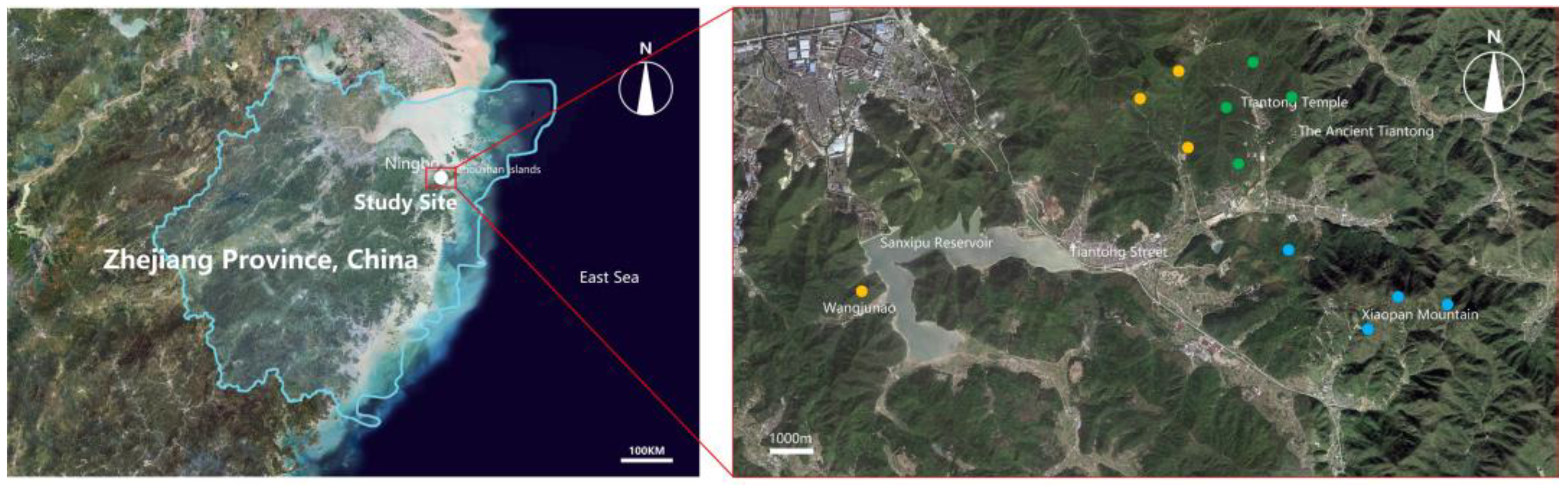
2.1. Study Site and Disturbance History

The study was conducted in the Tiantong National Forest Park (29°48′ N, 121°47′ E) of Zhejiang province, PR China (Figure 2). The region enjoys a subtropical monsoon climate with an average annual temperature of 16.2 °C and average annual precipitation of 1375 mm [25]. The soil in the sampling sites is typical acidic mountain yellow–red soil, with a pH value of about 4.5 to 5.0 and high in nitrogen and organic matter [26]. Vegetation is subtropical evergreen, broad-leaved forests. The typical overstory is dominated by Schima superba, Symplocos sumuntia, Machilus thunbergia, Symplocos stellaris, Camellia fraterna, Loropetalum chinense, Eurya muricate, and Eurya rubiginosa. In contrast, the understory layer is dominated by Diplopterygium glaucum, Woodwardia japonica, Indocalamus tessellatus, and Trachelospermum jasminoides.

The history of anthropogenic disturbance and forest conversion in the study area had been linked to forest clearance or selected logging for firewood. The mature forest was cleared but with many stumps remaining and then allowed to regrow [27]. The resultant vegetation is secondary evergreen and mixed deciduous forest developed through natural regeneration and resprouting. In a more intensive and repeatedly clear-cut area, secondary forests are characterized by shrublands developed through natural regeneration after the cessation of clear-cutting [28]. In more intensively clear-cut areas, entire vegetation was removed and planted with Chinese fir and bamboo. By contrast, the mature evergreen broadleaved forest had no history of intensive cutting around the Buddhist temple. Hence, intact mature forests, shrublands, and plantations form a natural gradient of increasing disturbance intensity [29]. The ages of mature forest sites are approximately 60 years, while the ages of shrublands and plantations are around 20 years.

2.2. Plot Establishment, Spatial Scaling, and Vegetation Sampling

We selected four replicate sites for each of the two disturbed forest types (shrubland and plantation) and control (intact mature forest) for 12 sites. Selected sites were geographically separated from each other by at least 150 m. At each site (n = 12), we first established a large plot of 20 m × 100 m. We then divided the large plot (20 m × 100 m) into five contiguous plots of 20 m × 20 m. We further divided each 20 m × 20 m plot into four plots of 10 m × 10 m. That is, we had one large 20 × 100 m² plot/site, five medium 20 × 20 m² plots/site, and 20 small 10 × 10 m² plots/site. In this plot design, smaller plots were nested within larger plots.

Small, medium, and large plots correspond to small, medium, and large spatial scales. Based on Fridley et al. [30], we anticipate that most individuals (cf. plants) can interact with each other at a “small scale” (10 × 10 m²), and within-plot environmental heterogeneity at a “small scale” is negligible. At a “medium scale” (20 × 20 m²), some individuals can interact with each other, and within-plot environmental heterogeneity is moderate; at a “large scale” (20 × 100 m²), the majority of individuals do not directly interact with more than a few individuals within their neighborhoods, and within-plot environmental heterogeneity is high. A previous study from the same forest reserve compared plant spatial patterns for 100 m² and 400 m² plot sizes and found relatively more robust signs of species interactions at a 100 m² than 400 m² scale [18], confirming the suitability of the adopted spatial-scaling schemes for the current study.

In June–October 2020–2021, we identified all woody and non-woody species and estimated their abundance (i.e., counted the number of individuals per species) for each of the small (n = 20 plots/site), medium (n = 5 plots/site), and large plots (n = 1 plot/site). However, abundance data from 5 medium or 20 small continuous plots for each site (n = 12) were later averaged to represent site-wise vegetation data for medium (20 m × 20 m) or small (10 m × 10 m) plots, respectively. Importantly, we sampled 5 to 20 medium and small plots per site to capture within-site variability in species richness and the composition from that specific scale, while we averaged these plots for each spatial scale to avoid the site-level pseudo-replication and spatial autocorrelation problems. This procedure resulted in four site-level mean replicates for each plot size (cf. spatial scale) and four replicates for each forest type.

2.3. Functional Traits

We considered seven leaf traits in this study: (i) specific leaf area (SLA), (ii) leaf dry matter content (LDMC), (iii) leaf thickness (LT), (iv) leaf succulence (LS), (v) leaf carbon content (LC), (vi) leaf nitrogen content (LN), and (vii) leaf phosphorus content (LP). These traits are important for understanding vegetation growth and dynamics, nutrient cycling, and forest regeneration: SLA is related to the plant growth rate [31,32]; LDMC is related to plant nutrient conservation [33]; LT is related to plant nutrient conservation, response to water deficits, and palatability to herbivores [34,35]; LS is related to plant leaves functioning well even though they temporarily lack an external water supply [36]. On the other hand, LC, LN, and LP concentrations are related to photosynthesis [37] and protein synthesis [38].

We followed Cornelissen et al. [39] for leaf trait measurements. In short, we collected three well-grown branches with their leaves for each species. Then, we selected ten mature leaves without any sign of physical damage from each branch and combined all leaves to form a composite sample of over 60 leaves per individual. We wrapped these leaves in moist paper, placed them into a sealed plastic bag, and kept those bags in a cooler until they were transported back to the laboratory within six hours. Next, we randomly selected ten mature leaves from each individual to weigh fresh leaf weight (l_fw) using an electric balance (BSA224S electronic scale, Sartorius Group, Beijing, China) and to measure leaf areas (l_area) using a leaf area meter (LI-3000C Portable Area Meter, LI-COR, Lincoln, NE, USA). Samples were then placed in an oven at 75 °C for 48 h to determine dry leaf weight (l_dw). We quantified SLA as l_area/l_dw, LDMC as l_dw/l_fw. LS was assessed as the ratio of values of fresh leaf weight, subtracting dry leaf weight from leaf area [40]. Leaf samples were then boiled with concentrated H₂SO₄ and H₂O₂ to oxidize and decompose leaf organic nitrogen and phosphorus. After the constant volume of dissolving solution, leaf nitrogen concentration (LN) was assessed following the Kjeldahl method [41]; leaf phosphorus concentration (LP) was assessed following the Mo-Sb anti-spectrophotometric method [42]. Leaf carbon concentration (LC) was assessed following potassium dichromate oxidation outside the heating method [43]. Trait–trait correlation among these leaf traits was relatively weak for most traits (Supporting Information, Figure S1), implying that the selected traits captured somewhat unique information concerning community functionality.

2.4. Quantifying Species and Functional Diversity and Composition

We quantified species richness, evenness and Shannon’s diversity to represent species diversity. While species richness refers to the number of unique species in a community (i.e., plot), species evenness can be quantified using at least 14 different indices, each having pros and cons [44,45]. We choose the Evar index of evenness for this because (i) Evar is more independent from richness (that is, it carries relatively unique information) than other evenness indexes [23] and (ii) Evar is equally sensitive to both abundant and rare species [44]. We computed Evar as per Equation (1) [44]:

$$E_{var}=1-\frac{2}{\mathsf{\pi }}\arctan \left\{\sum _{s=1}^S{\left(\ln \left(x_s\right)-\sum _{t=1}^S\ln \left(x_t\right)/S\right)}^2/S\right\}$$

(1)

where $x_s$ and $x_t$ refer to the number of individuals in species s or t, respectively, and S is the number of species. The variance is converted by $-2/\mathsf{\pi } \arctan \left( \right)$ to a 0–1 range with 0 representing the minimum species evenness and 1 meaning the maximum. Shannon’s species diversity was computed as per Equation (2) [46]:

$$\mathrm{H}=-\sum p_{i}ln\left({\mathrm{p}}_i\right)$$

(2)

where pi indicates the relative abundance of species i in the community.

To represent functional diversity and to make it comparable to species diversity, we quantified functional richness (FRic), functional evenness (FEve) and functional diversity (Rao’s Q). Although intraspecific variation can be an important factor in quantifying functional diversity [47,48], we focused on species-level trait mean for three reasons. First, quantifying plant elemental traits (i.e., leaf C, N and P) for many samples was a logistical challenge. Secondly, Ross et al. [49] suggest that ignoring intraspecific trait variation does not impact FRic and FEve, though Rao’s Q can be impacted. Thirdly, past work from the same forest found relatively slight intraspecies trait variation in woody species [12]. All functional diversity indices were calculated by using the function “dbFD” in the R library “FD” [50] and using Gower’s distance [51].

2.5. Quantifying Community-Level Functional Redundancy and Species-Level Functional Uniqueness

We quantified community-level functional redundancy and species-level functional uniqueness as per Equations (3) and (4) [14]:

$$Community-level functional redundancy=1-\frac{Q}{D}$$

(3)

$$Species-level functional uniqueess={\sum }_j\frac{p_j}{1-p_i}{\delta }_{ij}$$

(4)

where Q represents Rao’s quadratic entropy or mean functional dissimilarity and D represents the Simpson index of species diversity. On the other hand, $p_i$ and $p_j$ indicate the relative abundance of species i and j in the community, and ${\delta }_{ij}$ summarize the pairwise functional dissimilarities between species i and j and range from 0 to 1. Note that the idea of quantifying functional redundancy using Rao’s quadratic entropy and the Simpson index was first proposed by de Bello et al. [52] as the arithmetic difference between these two indices (D–Q). To ensure that our community-level functional redundancy calculations were not influenced by methodological choice, we repeated our community-level functional redundancy calculation by following de Bello, Lepš, Lavorel and Moretti [52]. Both community-level functional redundancy and species-level functional uniqueness were computed using the R codes and functions provided by Ricotta, de Bello, Moretti, Caccianiga, Cerabolini and Pavoine [14].

2.6. Statistical Analysis

To examine the empirical relationships between species richness versus functional richness, species evenness versus functional evenness, and Shannon’s species diversity versus Rao’s functional diversity and their potential dependence on disturbance and spatial scale, we conducted a series of linear mixed-effect model analyses (Zuur et al., 2009). Following our sampling design, we considered disturbance and spatial scale as fixed factors and site as a random factor in which spatial scales were nested. We conducted this analysis separately for the woody layer, the non-woody layer, and the woody plus non-woody layers combined.

The general linear mixed-effect model is:

$$\begin{gathered} \mathrm{Y}~ {\alpha }_1\mathrm{X} +{\alpha }_2\mathrm{disturbance} +{\alpha }_3\mathrm{spatial} \mathrm{scale} +{\alpha }_4\mathrm{X} \times \mathrm{disturbance} +{\alpha }_5\mathrm{X}\times \mathrm{spatial} \mathrm{scale}, \\ \mathrm{random} =1/\mathrm{site}/\mathrm{spatial} \mathrm{scale} \end{gathered}$$

(5)

where Y can be either functional richness, evenness or diversity in all species combined, woody species only and non-woody species only. An independent variable X corresponds to species richness, evenness or diversity of all species combined, woody species only and non-woody species only, and ${\alpha }_{1-5}$ represent regression coefficients. Disturbance refers to the mature forest, shrubland and plantation, and spatial scale refers to 10 m × 10 m, 20 m × 20 m, and 20 m × 100 m plot sizes. We transformed the species and functional diversity data into natural logarithms to reduce the skewness in the data; residual analyses confirmed that the transformations were generally successful in meeting the residual normality. In the equation mentioned above (Equation (5)), statistically significant interaction terms (e.g., $\mathrm{X}\times \mathrm{disturbance} \mathrm{or} \mathrm{X}\times \mathrm{spatial} \mathrm{scale}$ term in Equation (5)) would indicate significant slope differences among disturbances or spatial scales [5].

In the beginning, we included all relevant factors and interaction terms in the statistical model. Final models were selected based on the significance of a predictor term (α = 0.05) and the lowest Akaike information criterion (AIC) values (Burnham & Anderson 2002; Zuur et al., 2009).

We conducted similar mixed-effect modeling tests to examine whether community-level functional redundancy, species-level functional uniqueness and the community-weighted mean (CWM) of individual traits vary with disturbance and spatial scale. If a test revealed significant variation in community-level functional redundancy, species-level functional uniqueness and the community-weighted mean (CWM) of individual traits concerning disturbance or spatial scale, then we conducted the follow-up Tukey’s post-hoc test on the mixed model. All the statistical analyses were conducted in the statistical program R.

3. Results

Over the entire dataset, we detected 100 woody and 31 non-woody species for a total of 131 plant species in the study (Supporting Information, Table S1). The richness and diversity of species and functional traits were generally higher in the moderately-disturbed shrubland than in the mature forest or plantation, though shrublands were like the mature forests and plantations on several occasions (Figure 3). However, as the plot size increased, species and functional diversity increased, and the pattern was the opposite for evenness (Figure 4). Compositionally, the community-weighted mean leaf dry matter contents (LDMC), leaf thickness (LT), leaf succulence (LS), and leaf carbon contents (LC) varied significantly among disturbed versus undisturbed forests (Figure S2) but not among spatial scales of observation (Figure S3). In particular, the relatively intact mature forests had high LDMC but low LT, low LS, and high LC. By contrast, specific leaf area (SLA) and leaf nitrogen contents (LN) varied significantly among spatial scales but not forest types. The overall pattern of functional composition was consistent when we looked into it separately for woody and non-woody layers.

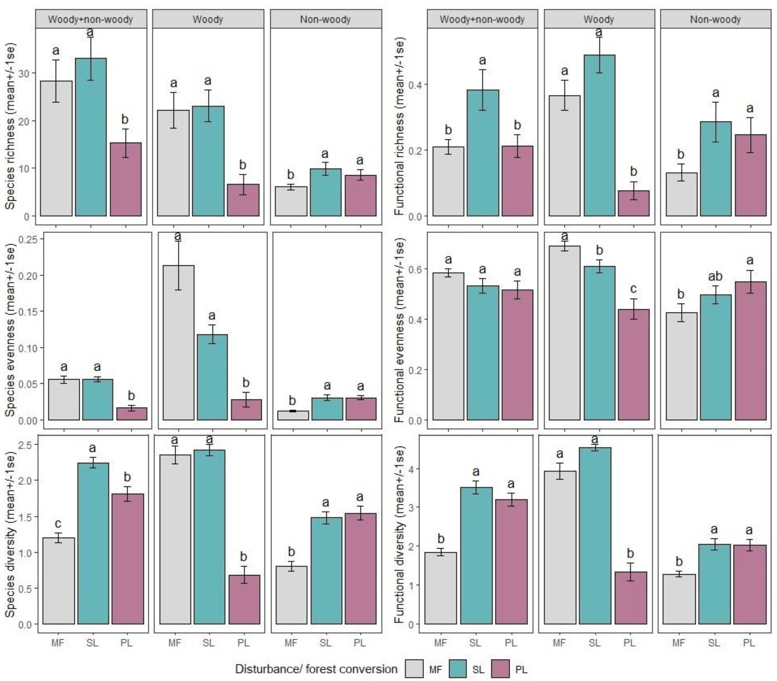
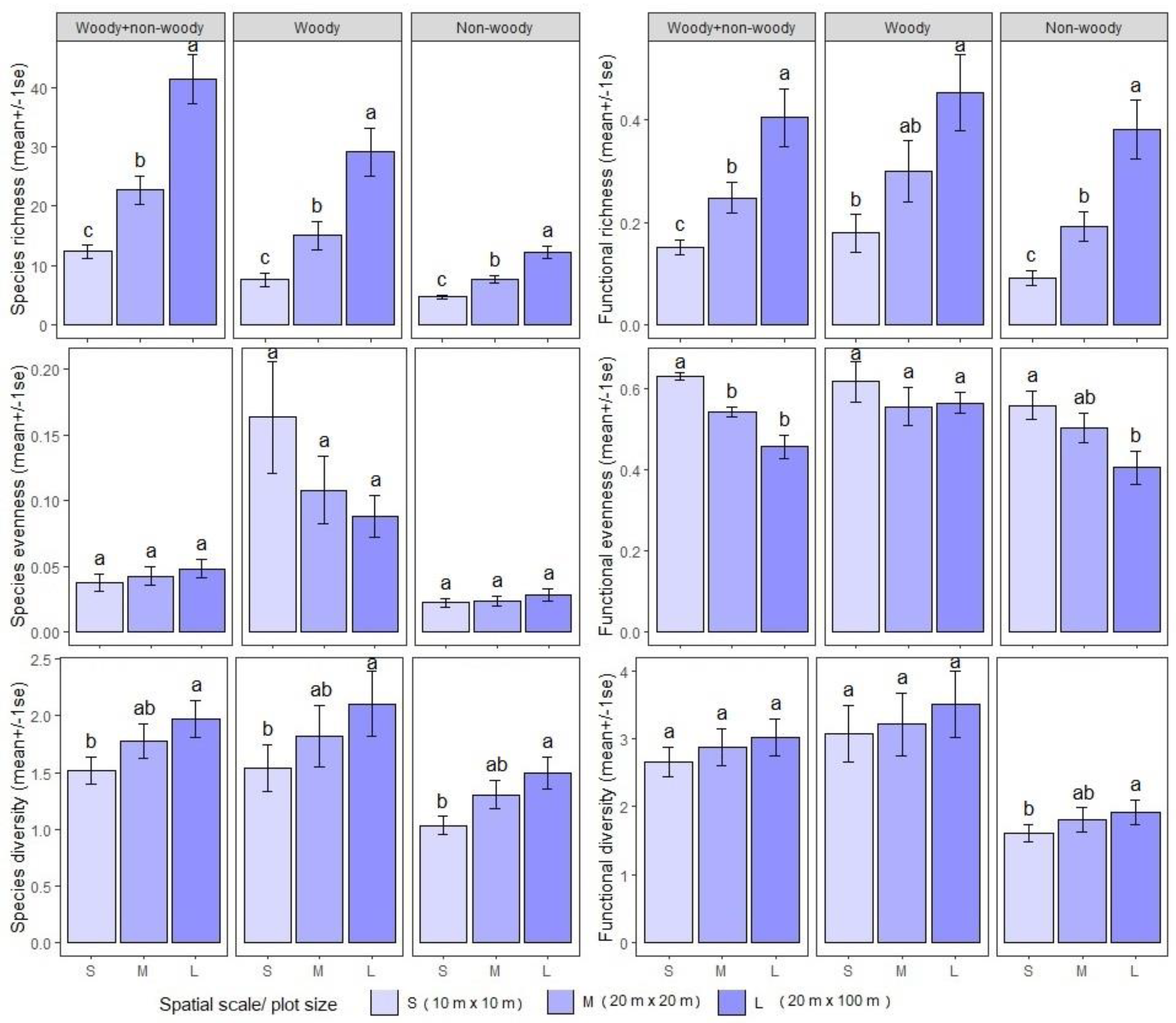
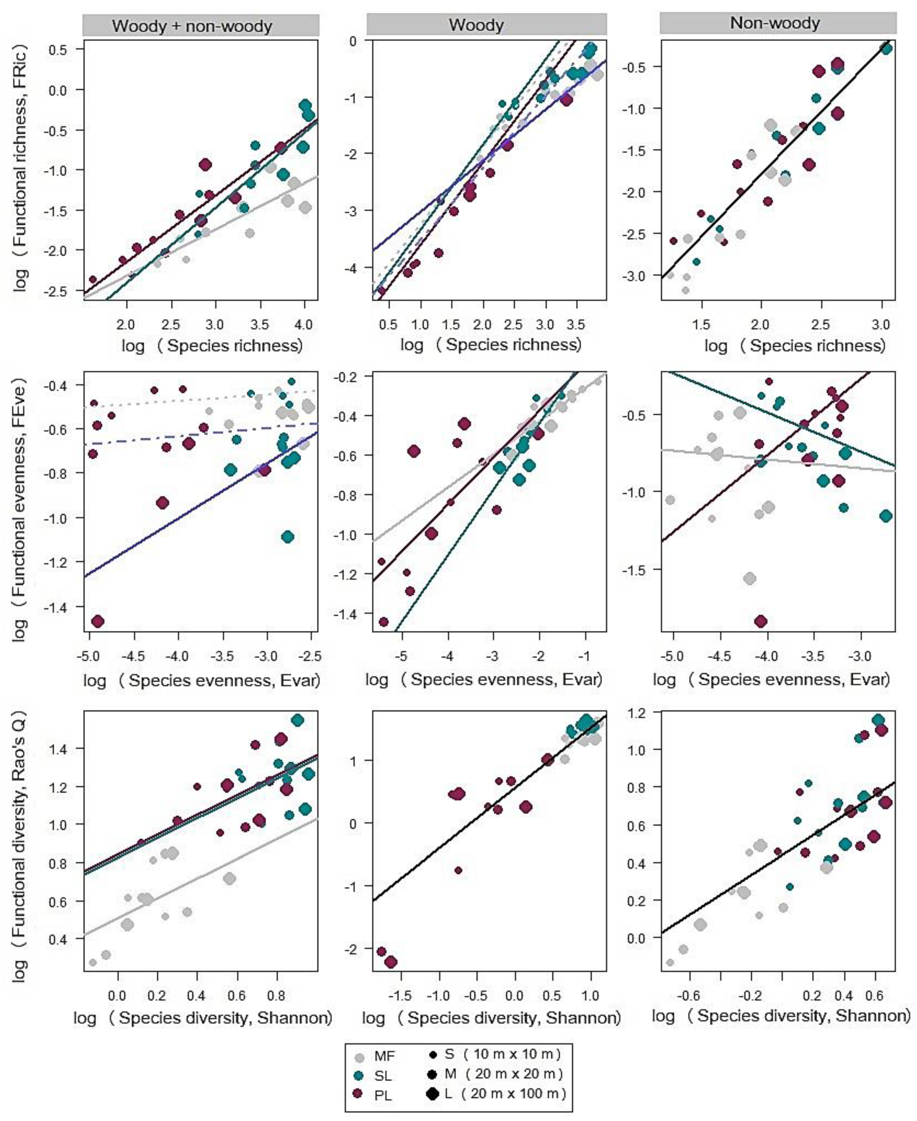
3.1. Species Richness Versus Functional Richness (FRic) Relationship

The overall (woody plus non-woody layers combined) species richness versus functional richness (FRic) relationship was positive, but the slope varied substantially among disturbed versus undisturbed forests (F_2,13 = 4.69, p = 0.03; Figure 5; Table S2). In particular, the slope was steeper in disturbed forests (slope β_plantations = 0.578 + 0.253; β_shrublands = 0.578 + 0.360) compared to that in intact mature forests (β_{intact mature forest} = +0.578). However, the results varied when the relationship was examined separately for woody and non-woody layers. For instance, the slope varied with both disturbance and spatial scale in the woody layer but did not vary with disturbance or spatial scale in the case of the non-woody layer (see Table S2). Nevertheless, the overall pattern of disturbance-mediated slope variation in the woody layer was consistent with that of woody plus non-woody layers combined: slopes for the woody layer also became slightly steeper in disturbed habitats (β_plantations = 1.368 + 0.092; β_shrublands = 1.368 + 0.138) than in intact mature forests (β_{intact mature forest} = +1.368). Interestingly, slopes in the woody layer became less steep as the plot size increased (β_{10 m × 10 m} = 1.368; β_{20 m × 20 m} = 1.368–0.098; β_{20 m × 100 m} = 1.368–0.469).

3.2. Species Evenness Versus Functional Evenness (FEve) Relationship

The overall species evenness versus functional evenness relationship was positive (Figure 5), but the slope increased with increasing plot size (β_{10 m × 10 m} = 0.029 versus β_{20 m × 20 m} = 0.029 + 0.009 versus β_{20 m × 100 m} = 0.029 + 0.220; Table S2). Contrary to our hypothesis, we did not detect any significant variation in slope among disturbed versus undisturbed forests.

Nevertheless, our hypothesized disturbance-dependent variations in the slope of the species’ evenness versus functional evenness relationship were evident when we assessed it separately for woody and non-woody layers (Table S2). For the woody layer, the slope was steeper in disturbed forests (βplantations = 0.167 + 0.070; βshrublands = 0.167 + 0.166) than in intact mature forests (βintact mature forest = +0.167). However, the non-woody layer’s slope was highly variable depending on the forests and even switched from positive to negative (βintact mature forest = −0.057; βplantations = +0.553–0.057; βshrublands = −0.057–0.198; Table S2). We failed to individually detect spatial-scale dependent variation in the species versus functional evenness relation for both woody and non-woody layers (p values > 0.05, see Table S2).

3.3. Species Diversity Versus Functional Diversity (RaoQ) Relationship

The overall relationship between Shannon’s species diversity and Rao’s functional diversity was positive, and the slope neither varied with disturbance nor spatial scale (Figure 5). When we looked into the relationship separately for woody and non-woody layers, we also failed to detect any variation in slope for disturbance or spatial scale.

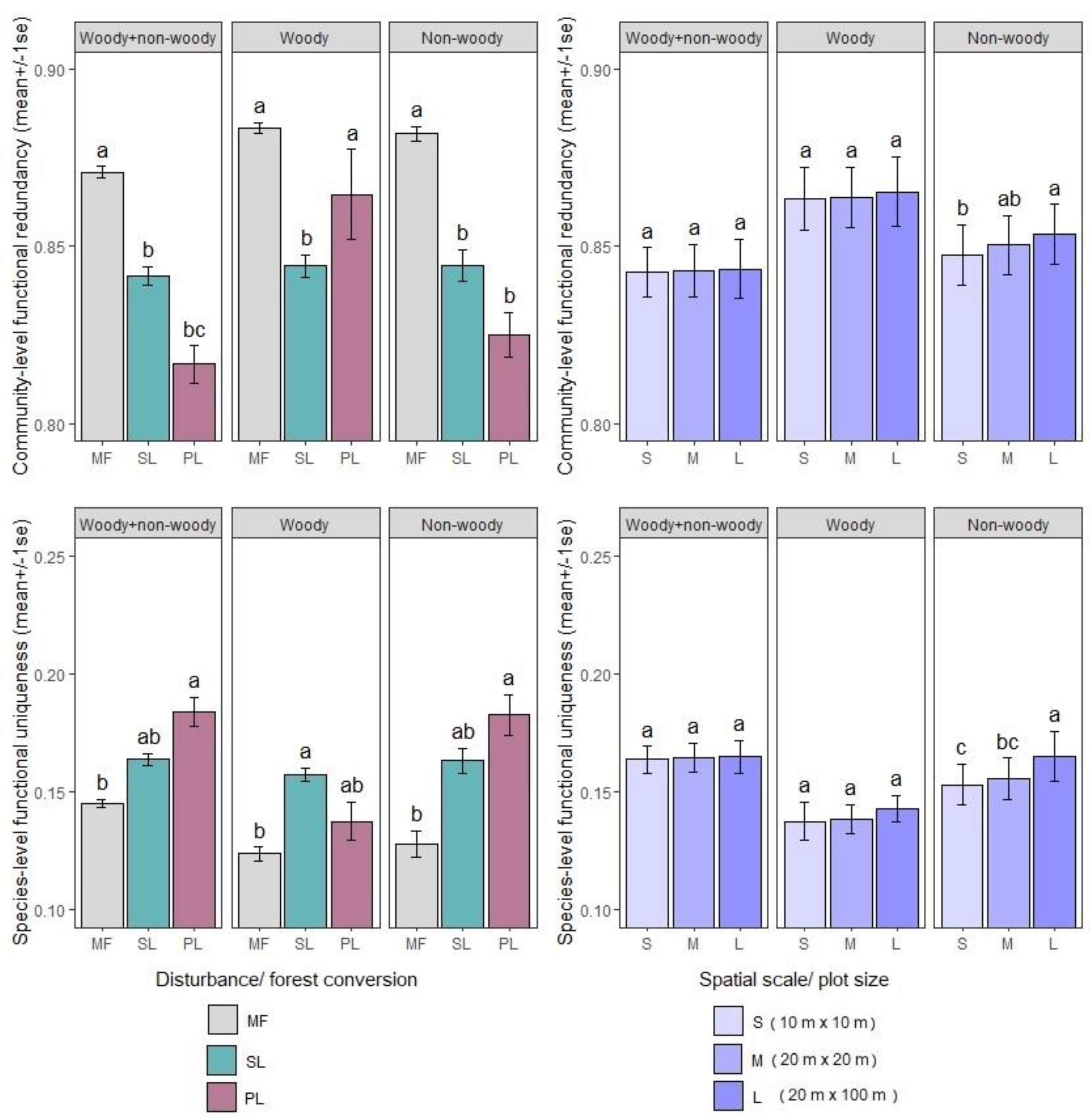
3.4. Community-Level Functional Redundancy and Species-Level Functional Uniqueness

The overall (woody plus non-woody layers combined) community-level functional redundancy varied markedly among disturbed versus undisturbed forests (mixed model ANOVA, F_2,9 = 15.93; p < 0.001) but not among spatial scales of observation (F_2,18 = 0.11; p = 0.90). Intact mature forest had higher community-level functional redundancy than the plantation or shrubland (Figure 6). When we looked into the pattern separately for woody and non-woody layers, we did not find any significant difference in community-level functional redundancy for either disturbed versus undisturbed forests (F_2,9 = 1.79; p = 0.22) or for different spatial scales (F_2,18 = 0.19; p = 0.83) in the woody layer. However, in the non-woody layer, we detected a substantially higher degree of community-level functional redundancy for the intact mature forests than for disturbed shrublands or plantations (F_2,9 = 11.52; p < 0.001).

4. Discussion

In this study, we set out to examine whether the different facets of the SD–FD relationship (species richness versus FRic; species evenness versus FEve; Shannon’s diversity versus Rao’s quadratic entropy) vary among disturbed versus undisturbed forests and whether the conclusion depends on the spatial scale of observation or vegetation layer. We found that the relationships between different facets of the species and functional diversity vary mainly among disturbed versus undisturbed forests and vegetation layers, partly due to disturbance-dependent variations in community-level functional redundancy and species-level functional uniqueness [7,8,9,14]. The scale dependence of the SD–FD relationship was evident only in the evenness component of the relationship in the woody layers. Below we discuss the roles of disturbance, spatial scale, and vegetation layers in modulating the SD–FD relationship and the implications of these results for forest management.

Our results of a generally positive relationship between different facets of the SD–FD relationships (Figure 5) are consistent with earlier studies [9,11,53,54]. It validates the assumption that the higher the species diversity, the more well-functioning and healthier the ecosystem [3,4]. However, relatively steeper slopes of the SD–FD relationships for disturbed than undisturbed forests underscore the importance of each added species to the overall functioning of the disturbed forests [5]. Indices of functional redundancy and uniqueness reflecting species’ importance to community functioning thus had lower values in disturbed than undisturbed forests (Figure 6). In particular, the relatively intact mature forests were characterized by redundant species having high LDMC but low LT, low LS, and high LC, and vice versa for disturbed forests (Figure S3). While past research that included a mixture of competitive, generalist, and disturbance-responsive traits found high functional redundancy in disturbed habitats [9], our chosen traits mainly included resource acquisition or conservation traits related to competition. As a result, we found higher functional redundancy in undisturbed than disturbed forests, contrary to our hypothesis or earlier studies. This result suggests that the choice of traits can significantly influence the patterns and drivers of the SD–FD relationship. Nevertheless, our findings of the steeper slopes in the SD–FD relationship coupled with low functional redundancy or uniqueness imply that disturbed habitats are susceptible to losing certain functions altogether in the event of the loss of a few species [11].

Although we evaluated disturbance response to different dimensions of the SD–FD relationship, we failed to detect a consistent pattern: the richness relationship showed a solid response to disturbance, evenness showed a weak response, and the aggregated diversity relationship showed no response. While the richness relationship focuses on the link between the number of species and the volume of functional space, the evenness relationship focuses on species abundance distribution versus the regularity of trait distributions [55]. Disturbance-driven altered site conditions or propagule scarcity could limit the presence of species and thus impact the richness relationship. By contrast, the abundance of species and functional traits are sensitive to localized variation in site conditions and the presence of competitors [56], so the evenness relationship could vary widely and differ from the richness relationship. On the other hand, the aggregated diversity relationship focuses on the overall richness and evenness variation together. We suspect that the differential response of richness and evenness to disturbance might have masked the overall disturbance response in the aggregated diversity relationship.

However, compared to widespread and strong disturbance effects, we found somewhat weak and limited effects of spatial scale in modulating the SD–FD relationship. We detected relatively steeper slopes of the SD–FD relationship with increasing spatial scale in only two instances. The first instance was the woody layer’s species richness versus FRic relationship, while the second case was the species evenness versus FEve relationship in the woody and non-woody layers combined. However, unlike the disturbance-dependent variation in functional redundancy or uniqueness, we failed to detect scale-dependent variation in functional redundancy or uniqueness to explain any such variation in the SD–FD relationship. We suspect that local-scale variation in site environmental factors might be an important driver of species abundance and, in turn, the species evenness versus FEve relationship [57]. Future studies may thus account for the variation in site environmental conditions while assessing the relationship.

Meanwhile, the effects of disturbance or spatial scale on the SD–FD relationship seem inconsistent across vegetation layers. For instance, while the effect of disturbance and spatial scale on the richness relationship was striking in the woody layer, no such effect was evident for the non-woody layer. Similarly, the disturbance effect on the evenness relationship was positive in the woody layer but highly variable in the non-woody layer. Such variation in the SD–FD relationship is not surprising for two reasons. Firstly, a disturbance may not impact woody and non-woody vegetation similarly. Secondly, woody and non-woody vegetation have different resource requirements and respond to disturbances differently. As a result, community-level functional redundancy or species-level functional uniqueness differed markedly, potentially causing vegetation-layer-dependent variation in the SD–FD relationship.

Implications for Forest Management and Conservation

Ecosystem managers, such as forest managers, traditionally rely on species diversity to assess the health of their managed systems. The positive SD–FD relationship from our study confirms the usefulness of such an approach. Practitioners can utilize the SD–FD relationship to assess the health of their managed forests relative to undisturbed forests. However, disturbance-, spatial-scale-, or vegetation-layer-dependent variation in the SD–FD relationship coupled with differential patterns of functional redundancy or uniqueness underscores the potential risks of sole reliance on species diversity. For instance, disturbed habitats are susceptible to losing certain functions altogether in the event of the loss of a few species, and species diversity alone cannot foresee this risk in advance. We, therefore, join with other researchers and call for the utilization of both species and functional diversity simultaneously to monitor ecosystem health. More specifically, we suggest periodic monitoring of species versus functional diversity relationships as indicators of ecosystem functions and stability [9]. At the same time, vegetation-layer-dependent variation in the SD–FD relationship reminds us to consider the woody and non-woody layers separately while assessing the status of a forest ecosystem. The context-dependent nature of the relationship also indicates that a cautious approach is needed while extrapolating the idea across systems.

References

1. Pereira, H.M.; Leadley, P.W.; Proença, V.; Alkemade, R.; Scharlemann, J.P.W.; Fernandez-Manjarrés, J.F.; Araújo, M.B.; Balvanera, P.; Biggs, R.; Cheung, W.W.L.; et al. Scenarios for Global Biodiversity in the 21st Century. Science 2010, 330, 1496–1501. [Google Scholar] [CrossRef] [PubMed] [Green Version]
2. Cadotte, M.W.; Carscadden, K.; Mirotchnick, N. Beyond species: Functional diversity and the maintenance of ecological processes and services. J. Appl. Ecol. 2011, 48, 1079–1087. [Google Scholar]
3. Hector, A.; Bagchi, R. Biodiversity and ecosystem multifunctionality. Nature 2007, 448, 188–190. [Google Scholar] [CrossRef] [PubMed]
4. Tilman, D.; Wedin, D.; Knops, J. Productivity and sustainability influenced by biodiversity in grassland ecosystems. Nature 1996, 379, 718–720. [Google Scholar] [CrossRef]
5. Biswas, S.R.; Mallik, A.U.; Braithwaite, N.T.; Biswas, P.L. Effects of disturbance type and microhabitat on species and functional diversity relationship in stream-bank plant communities. For. Ecol. Manag. 2019, 432, 812–822. [Google Scholar] [CrossRef]
6. Mayfield, M.M.; Boni, M.F.; Daily, G.C.; Ackerly, D. Species and functional diversity of native and human-dominated plant communities. Ecology 2005, 86, 2365–2372. [Google Scholar] [CrossRef] [Green Version]
7. Mayfield, M.M.; Bonser, S.P.; Morgan, J.W.; Aubin, I.; McNamara, S.; Vesk, P.A. What does species richness tell us about functional trait diversity? Predictions and evidence for responses of species and functional trait diversity to land-use change. Glob. Ecol. Biogeogr. 2010, 19, 423–431. [Google Scholar] [CrossRef]
8. Sasaki, T.; Okubo, S.; Okayasu, T.; Jamsran, U.; Ohkuro, T.; Takeuchi, K. 1-208. Two-phase functional redundancy in plant communities along a grazing gradient in Mongolian rangelands. Ecology 2009, 90, 2598–2608. [Google Scholar] [CrossRef] [Green Version]
9. Biswas, S.R.; Mallik, A.U. Species diversity and functional diversity relationship varies with disturbance intensity. Ecosphere 2011, 2, art52. [Google Scholar] [CrossRef]
10. Carmona, C.P.; Azcárate, F.M.; de Bello, F.; Ollero, H.S.; Lepš, J.; Peco, B. Taxonomical and functional diversity turnover in Mediterranean grasslands: Interactions between grazing, habitat type and rainfall. J. Appl. Ecol. 2012, 49, 1084–1093. [Google Scholar] [CrossRef]
11. Dovrat, G.; Meron, E.; Shachak, M.; Moshe, Y.; Osem, Y. The relationship between species diversity and functional diversity along aridity gradients in semi-arid rangeland. J. Arid Environ. 2021, 195, 104632. [Google Scholar] [CrossRef]
12. Ouyang, J.; Biswas, S.R.; Yin, C.; Qing, Y.; Biswas, P.L. Shifting Importance of Abiotic versus Biotic Filtering from Intact Mature Forests to Post-Clearcut Secondary Forests. Forests 2022, 13, 672. [Google Scholar] [CrossRef]
13. Chazdon, R.L. Second Growth: The Promise of Tropical Forest Regeneration in an Age of Deforestation; University of Chicago Press: Chicago, IL, USA, 2014. [Google Scholar]
14. Ricotta, C.; de Bello, F.; Moretti, M.; Caccianiga, M.; Cerabolini, B.E.L.; Pavoine, S. Measuring the functional redundancy of biological communities: A quantitative guide. Methods Ecol. Evol. 2016, 7, 1386–1395. [Google Scholar] [CrossRef] [Green Version]
15. Li, H. Scale-Dependent Effects of Forest Conversion on Species and Functional Diversity in Zhejiang Tiantong National Forest Park; East China Normal University: Shanghai, China, 2021. [Google Scholar]
16. Wiens, J.A. Spatial Scaling in Ecology. Funct. Ecol. 1989, 3, 385–397. [Google Scholar] [CrossRef]
17. Levin, S.A. The Problem of Pattern and Scale in Ecology: The Robert H. MacArthur Award Lecture. Ecology 1992, 73, 1943–1967. [Google Scholar] [CrossRef]
18. Xiang, J. Effects of Forest Conversion on Spatial Aotocorrelation in Plant Species and Functional Diversity in Tiantong National Forest Park; East China Normal University: Shanghai, China, 2021. [Google Scholar]
19. Fletcher, R.; Fortin, M.-J. Scale. In Spatial Ecology and Conservation Modeling: Applications with R; Springer International Publishing: Cham, Switzerland, 2018; pp. 17–53. [Google Scholar] [CrossRef]
20. Albert, C.H.; Grassein, F.; Schurr, F.M.; Vieilledent, G.; Violle, C. When and how should intraspecific variability be considered in trait-based plant ecology? Perspect. Plant Ecol. Evol. Syst. 2011, 13, 217–225. [Google Scholar] [CrossRef]
21. McGuinness, K.A. Species–area curves. Biol. Rev. 1984, 59, 423–440. [Google Scholar] [CrossRef]
22. Chen, H.Y.H.; Biswas, S.R.; Sobey, T.M.; Brassard, B.W.; Bartels, S.F. Reclamation strategies for mined forest soils and overstorey drive understorey vegetation. J. Appl. Ecol. 2018, 55, 926–936. [Google Scholar] [CrossRef]
23. Stirling, G.; Wilsey, B. Empirical Relationships between Species Richness, Evenness, and Proportional Diversity. Am. Nat. 2001, 158, 286–299. [Google Scholar] [CrossRef]
24. Villeger, S.; Mason, N.W.H.; Mouillot, D. New multidimensional functional diversity indices for a multifaceted framework in functional ecology. Ecology 2008, 89, 2290–2301. [Google Scholar] [CrossRef] [Green Version]
25. Wu, Y.-Y.; Guo, C.-Z.; Ni, J. Dynamics of major forest vegetations in Tiantong National Forest Park during the last 30 years. Chin. J. Appl. Ecol. 2014, 25, 1547–1554. (In Chinese) [Google Scholar]
26. Zhang, S.; Zeng, Y.; He, Y.; Chen, Y.; Lu, J.; Liu, H.; Xu, M.; Wang, X. Spatiotemporal distribution characteristics of leaf-litter nutrients in a dynamic plot of subtropical evergreen broad-leaved forest in Tiantong, Zhejiang Province. Acta Ecol. Sin. 2020, 40, 7335–7342. [Google Scholar]
27. Wang, X.-H.; Kent, M.; Fang, X.-F. Evergreen broad-leaved forest in Eastern China: Its ecology and conservation and the importance of resprouting in forest restoration. For. Ecol. Manag. 2007, 245, 76–87. [Google Scholar] [CrossRef]
28. Yan, E.-R.; Wang, X.-H.; Huang, J.-J. Shifts in plant nutrient use strategies under secondary forest succession. Plant Soil 2006, 289, 187–197. [Google Scholar] [CrossRef]
29. Yan, E.-R.; Wang, X.-H.; Guo, M.; Zhong, Q.; Zhou, W.; Li, Y.-F. Temporal patterns of net soil N mineralization and nitrification through secondary succession in the subtropical forests of eastern China. Plant Soil 2009, 320, 181–194. [Google Scholar] [CrossRef]
30. Fridley, J.D.; Stachowicz, J.J.; Naeem, S.; Sax, D.F.; Seabloom, E.W.; Smith, M.D.; Stohlgren, T.J.; Tilman, D.; Holle, B.V. The invasion paradox: Reconciling pattern and process in species invasions. Ecology 2007, 88, 3–17. [Google Scholar] [CrossRef] [Green Version]
31. Adler, P.B.; Salguero-Gomez, R.; Compagnoni, A.; Hsu, J.S.; Ray-Mukherjee, J.; Mbeau-Ache, C.; Franco, M. Functional traits explain variation in plant life history strategies. Proc. Natl. Acad. Sci. USA 2014, 111, 740–745. [Google Scholar] [CrossRef] [Green Version]
32. Reich, P.B.; Walters, M.B.; Ellsworth, D.S. From tropics to tundra: Global convergence in plant functioning. Proc. Natl. Acad. Sci. USA 1997, 94, 13730–13734. [Google Scholar] [CrossRef] [Green Version]
33. Garnier, E.; Cortez, J.; Billes, G.; Navas, M.L.; Roumet, C.; Debussche, M.; Laurent, G.; Blanchard, A.; Aubry, D.; Bellmann, A.; et al. Plant functional markers capture ecosystem properties during secondary succession. Ecology 2004, 85, 2630–2637. [Google Scholar] [CrossRef]
34. Gratani, L.; Varone, L.; Crescente, M.F.; Catoni, R.; Ricotta, C.; Puglielli, G. Leaf thickness and density drive the responsiveness of photosynthesis to air temperature in Mediterranean species according to their leaf habitus. J. Arid Environ. 2018, 150, 9–14. [Google Scholar] [CrossRef]
35. Pauli, D.; White, J.W.; Andrade-Sanchez, P.; Conley, M.M.; Heun, J.; Thorp, K.R.; French, A.N.; Hunsaker, D.J.; Carmo-Silva, E.; Wang, G.; et al. Investigation of the Influence of Leaf Thickness on Canopy Reflectance and Physiological Traits in Upland and Pima Cotton Populations. Front. Plant Sci. 2017, 8, 1405. [Google Scholar] [CrossRef] [PubMed] [Green Version]
36. Eggli, U.; Nyffeler, R.; Eggli, U.; Nyffeler, R. Living under temporarily arid conditions-succulence as an adaptive strategy. Bradleya 2009, 27, 13–36. [Google Scholar] [CrossRef]
37. Hunt, E.R.; Weber, J.A.; Gates, D.M. Effects of Nitrate Application on Amaranthus powellii Wats. III. Optimal Allocation of Leaf Nitrogen for Photosynthesis and Stomatal Conductance. Plant Physiol. 1985, 79, 619–624. [Google Scholar] [CrossRef] [PubMed] [Green Version]
38. Reich, P.B.; Oleksyn, J. Global patterns of plant leaf N and P in relation to temperature and latitude. Proc. Natl. Acad. Sci. USA 2004, 101, 11001–11006. [Google Scholar] [CrossRef] [PubMed] [Green Version]
39. Cornelissen, J.H.C.; Lavorel, S.; Garnier, E.; Diaz, S.; Buchmann, N.; Gurvich, D.E.; Reich, P.B.; ter Steege, H.; Morgan, H.D.; van der Heijden, M.G.A.; et al. A handbook of protocols for standardised and easy measurement of plant functional traits worldwide. Aust. J. Bot. 2003, 51, 335–380. [Google Scholar] [CrossRef] [Green Version]
40. Mantovani, A. A method to improve leaf succulence quantification. Braz. Arch. Biol. Technol. 1999, 42, 9–14. [Google Scholar] [CrossRef] [Green Version]
41. Licon, C. Proximate and other chemical analyses. In Encyclopedia of Dairy Sciences, 3rd ed.; McSweeney, P.L.H., McNamara, J.P., Eds.; Academic Press: Oxford, UK, 2022; pp. 521–529. [Google Scholar] [CrossRef]
42. Guo, H.-N.; Wang, L.-X.; Liu, H.-T. Potential mechanisms involving the immobilization of Cd, As and Cr during swine manure composting. Sci. Rep. 2020, 10, 16632. [Google Scholar] [CrossRef]
43. Nelson, D.W.; Sommers, L. A Rapid and Accurate Procedure for Estimation of Organic Carbon in Soils; Indiana Academy of Science: Indianapolis, IN, USA, 1974; pp. 456–462. [Google Scholar]
44. Smith, B.; Wilson, J.B. A consumer’s guide to evenness indices. Oikos 1996, 76, 70–82. [Google Scholar] [CrossRef]
45. Tuomisto, H. An updated consumer’s guide to evenness and related indices. Oikos 2012, 121, 1203–1218. [Google Scholar] [CrossRef]
46. Shannon, C.E. A mathematical theory of communication. Bell Syst. Tech. J. 1948, 27, 379–423. [Google Scholar] [CrossRef] [Green Version]
47. Albert, C.H.; de Bello, F.; Boulangeat, I.; Pellet, G.; Lavorel, S.; Thuiller, W. On the importance of intraspecific variability for the quantification of functional diversity. Oikos 2012, 121, 116–126. [Google Scholar] [CrossRef]
48. Violle, C.; Enquist, B.J.; Mcgill, B.J.; Jiang, L.; Albert, C.H.; Hulshof, C.; Jung, V.; Messier, J. The return of the variance: Intraspecific variability in community ecology. Trends Ecol. Evol. 2012, 27, 244–252. [Google Scholar] [CrossRef] [PubMed]
49. Ross, S.R.P.-J.; Hassall, C.; Hoppitt, W.J.E.; Edwards, F.A.; Edwards, D.P.; Hamer, K.C. Incorporating intraspecific trait variation into functional diversity: Impacts of selective logging on birds in Borneo. Methods Ecol. Evol. 2017, 8, 1499–1505. [Google Scholar] [CrossRef] [Green Version]
50. Laliberte, E.; Legendre, P. A distance-based framework for measuring functional diversity from multiple traits. Ecology 2010, 91, 299–305. [Google Scholar] [CrossRef]
51. Gower, J.C. Principal coordinates analysis. In Encyclopedia of Biostatistics; Armitage, P., Colton, T., Eds.; John Wiley & Sons, Ltd.: Chichester, UK, 2005. [Google Scholar]
52. de Bello, F.; Lepš, J.; Lavorel, S.; Moretti, M. Importance of species abundance for assessment of trait composition: An example based on pollinator communities. Community Ecol. 2007, 8, 163–170. [Google Scholar] [CrossRef]
53. Warring, B.; Cardoso, F.C.G.; Marques, M.C.M.; Varassin, I.G. Functional diversity of reproductive traits increases across succession in the Atlantic forest. Rodriguésia 2016, 67, 321–333. [Google Scholar] [CrossRef] [Green Version]
54. Camilo, G.d.S.; Terra, B.d.F.; Araujo, F.G. Using the relationship between taxonomic and functional diversity to assess functional redundancy in streams of an altered tropical watershed. Environ. Biol. Fishes 2018, 101, 1395–1405. [Google Scholar] [CrossRef]
55. Mason, N.W.H.; Mouillot, D.; Lee, W.G.; Wilson, J.B. Functional richness, functional evenness and functional divergence: The primary components of functional diversity. Oikos 2005, 111, 112–118. [Google Scholar] [CrossRef]
56. Hillebrand, H.; Bennett, D.M.; Cadotte, M.W. Consequences of dominance: A review of evenness effects on local and regional ecosystem processes. Ecology 2008, 89, 1510–1520. [Google Scholar] [CrossRef]
57. Bergholz, K.; May, F.; Giladi, I.; Ristow, M.; Ziv, Y.; Jeltsch, F. Environmental heterogeneity drives fine-scale species assembly and functional diversity of annual plants in a semi-arid environment. Perspect. Plant Ecol. Evol. Syst. 2017, 24, 138–146. [Google Scholar] [CrossRef]
Figure 1. Hypothesized patterns of variations in community-level functional redundancy, species-level functional uniqueness, and the resultant variations in the species and functional diversity relationship concerning habitat disturbance (MF = mature forests, SL = shrublands and PL = plantations), spatial scale (L = large scale, M = medium scale and S = small scale) and vegetation layers (W = woody layers and NW = non-woody layers).
Forests 14 00408 g001
Figure 2. Map showing locations of study sites representing different types of disturbance (green = mature forests, yellow = shrublands, and blue = plantations).
Forests 14 00408 g002
Figure 3. Variations in the mean values (±1se) of different facets of species and functional diversity concerning habitat disturbance (MF = mature forests, SL = shrublands and PL = plantations) and vegetation layers. Bars marked with the same letters do not differ significantly at α = 0.05, as identified by Tukey’s post-hoc test.
Forests 14 00408 g003
Figure 4. Variations in the mean values (±1se) of different facets of species and functional diversity concerning spatial scale (L = large scale, M = medium scale and S = small scale) and vegetation layers. Bars marked with the same letters do not differ significantly at α = 0.05, as identified by Tukey’s post-hoc test.
Forests 14 00408 g004
Figure 5. Variations in the species versus functional diversity relationships concerning habitat disturbance (MF = mature forests, SL = shrublands and PL = plantations), spatial scale (L = large scale, M = medium scale and S = small scale), and vegetation layers. When a mixed-effect model (Equation (5)) shows a significant interaction effect concerning disturbance (X × disturbance) or spatial scale (X × spatial scale), we fitted separate lines (i.e., separate slopes and intercepts) for disturbance or spatial scale; when both disturbance and spatial scale show a significant effect, we fitted six lines (three for disturbance and three for spatial scale); when the interaction effect was non-significant, but disturbance or spatial scale effect was significant, we fitted different lines with a different intercept but a common slope; when the model shows only a significant effect concerning species diversity, we fitted a single line. Concerning disturbance effects, a grey line represents mature forests, blue represents shrublands and red represents plantations; concerning the spatial scale effects, a fainted line represents small scale, intermittently dotted lines represent medium scale, and solid lines represent large scale. See Table S2 for detailed statistical results.
Forests 14 00408 g005
Figure 6. Variations in the species versus functional diversity relationships concerning habitat disturbance, spatial scale, and vegetation layers. Bars marked with the same letters do not differ significantly at α = 0.05, as identified by Tukey’s post-hoc test. See Table S2 for detailed statistical results.
Forests 14 00408 g006
Disclaimer/Publisher’s Note: The statements, opinions and data contained in all publications are solely those of the individual author(s) and contributor(s) and not of MDPI and/or the editor(s). MDPI and/or the editor(s) disclaim responsibility for any injury to people or property resulting from any ideas, methods, instructions or products referred to in the content.