The Multivariate Distribution of Stand Spatial Structure and Tree Size Indices Using Neighborhood-Based Variables in Coniferous and Broad Mixed Forest

Abstract

The spatial structure of forest stands significantly influences inter-tree competition and the overall stability of the stand’s ecological dynamics, and a profound understanding of forest stand spatial structure is essential for both effective forest management and ecological research. Previous studies on spatial structure have primarily employed single variables, offering only one-dimensional structural insights and lacking the capacity to interpret multidimensional information. In light of these limitations, our study introduces a novel approach founded on a six-variable distribution, aimed at conducting a comprehensive analysis and interpretation of the spatial attributes of forest stands. Diverging from conventional univariate or bivariate methods, the hexi-variate approach simultaneously considers six variables, facilitating a more intricate exploration of the intricate interrelationships within forest ecosystems from six distinct dimensions. We conducted an in-depth analysis of the spatial structural attributes within the forest stand, encompassing factors such as species diversity, size variation, spatial distribution patterns, openness, vertical stratification, and stand competition. To capture a comprehensive view of the trees’ spatial information, we employed the hexadecimal distribution method, effectively quantifying their characteristics across six dimensions. Our study unveiled a significant correlation between spatial structure and stand growth, establishing a connection by integrating the spatial structure with key structural features relevant to tree size. The outcomes of this study shed light on the effectiveness and superiority of the six-element distribution method when it comes to the analysis of forest structural characteristics. Our approach offers valuable insights into the optimization of forest management strategies, encompassing selective harvesting and biodiversity conservation, thereby establishing a solid footing for sustainable forest management practices.

1. Introduction

Forest structure encompasses the arrangement and relationships of individual plants within a forest ecosystem. It serves as the cornerstone and most fundamental attribute of forest ecosystems, emerging from the intricate interplay of various natural ecological processes across spatial and temporal scales [1]. This structure is intricately linked to the functions and services that forests provide. Forest structure (distribution of trees and their attributes in space in forests) has significant theoretical and practical implications in maintaining biodiversity, promoting ecosystem function, and forest ecosystem management [2,3]. Enhancing the diversity and complexity of forest structure is widely recognized as an effective measure for safeguarding biodiversity within forest ecosystems and enhancing their overall productivity, as well as an effective means to precisely augment forest quality [4].

There is a wide range of forest structural elements, which can be classified as either spatial or non-spatial, also known as distance-dependent and distance-independent indicators, depending on whether they are related to the relative positioning of the stand [5,6]. Non-spatial structural characteristics encompass aspects such as tree species composition, diameter distribution, tree height distribution, age distribution, and tree density. Spatial structural characteristics, on the other hand, encompass factors like the degree of tree species mixing, size diversity, spatial distribution pattern, canopy openness, vertical stratification, and stand-level competition [7,8]. These elements are interconnected and interact with each other, resulting in complex heterogeneity and diversity within forest structure. A quantitative description of forest structure plays a pivotal role in unveiling the underlying structural principles and essential features of forests [9]. This, in turn, facilitates the development of targeted strategies for regulating forest structure and the formulation of sound forest management practices, ultimately contributing to the promotion of the health and stability of forest ecosystems [10].

Quantitative description methods, complemented by intuitive visual representations, significantly enhance our understanding and grasp of forest structure, thus providing valuable insights and guidance for the implementation of effective forest management practices [11,12]. Currently, a diverse array of indicators and methodologies for characterizing stand structure can be categorized or subdivided based on spatial and temporal dimensions of stand structure, as well as the consideration of stand position within the landscape [13]. Among these techniques, spatial structural parameters derived from nearest-neighbor relationships succinctly capture stand structure [14]. Previous studies predominantly relied on mean values of these parameters and their one-dimensional distributions to depict the overall or one-sided spatial structural characteristics of forest stands [15,16,17]. However, these approaches can only provide an overall or one-dimensional view of stand structure, neglecting other vital aspects of spatial structural information. To enhance our understanding of forest structure and harness the potential utility of these structural parameters in forest management, it is essential to develop a comprehensive and systematic approach for interpreting the inherent heterogeneity within forest spatial structure.

The currently most utilized spatial structural parameters, including mingling degree, angular scale, and size ratio number, are employed to elucidate the spatial characteristics of individual aspects within a stand comprising four nearest neighboring trees, each categorized into five distinct value classes (i.e., 0.00, 0.25, 0.50, 0.75, and 1.00) [18]. Consequently, these two features, both independent and quantifiably finite, establish the fundamental prerequisites for satisfying the joint probability distribution of spatial structural parameters within an N-element distribution. Zhang et al. introduced a quadratic distribution model to analyze the spatial structural heterogeneity of forest stands [19]. This approach yielded more direct and valuable insights into forest structure heterogeneity compared to prior methods, including ternary, binary, monodistribution, zero-distribution (mean), and other conventional techniques. However, these investigations did not encompass crucial aspects of spatial structure, such as parameters like forest layer index, degrees of freedom, and openness ratio. Incorporating these additional parameters into the N-element distribution of spatial structural parameters and exploring more comprehensive quantitative analysis methods for forest spatial structure have the potential to significantly enhance our comprehension of spatial structural heterogeneity and diversity within small-scale forests. The N-variate distribution analysis of spatial structural parameters provides a more comprehensive and intuitive dataset in comparison to traditional univariate methods when examining spatial structural attributes.

The present study was carried out within nine 20 m × 30 m permanent fixed plots situated in a mixed forest of cunninghamia lanceolata and phoebe bournei (CLPB) located on Jindong Forest Farm. The spatial structure characteristics of CLPB and the relationship between spatial structure and tree size were analyzed using the multivariate distribution method with sample plot survey data. Our study was driven by three principal objectives: (1) validate the accuracy and effectiveness of the six-variable distribution method in providing a systematic and comprehensive evaluation of forest spatial structure and compare its superiority to the univariate distribution method, (2) examine the relationship between forest spatial structure and forest growth, and (3) demonstrate the applicability of the six-variable distribution method in forest structure adjustment and thinning operations.

2. Materials and Methods

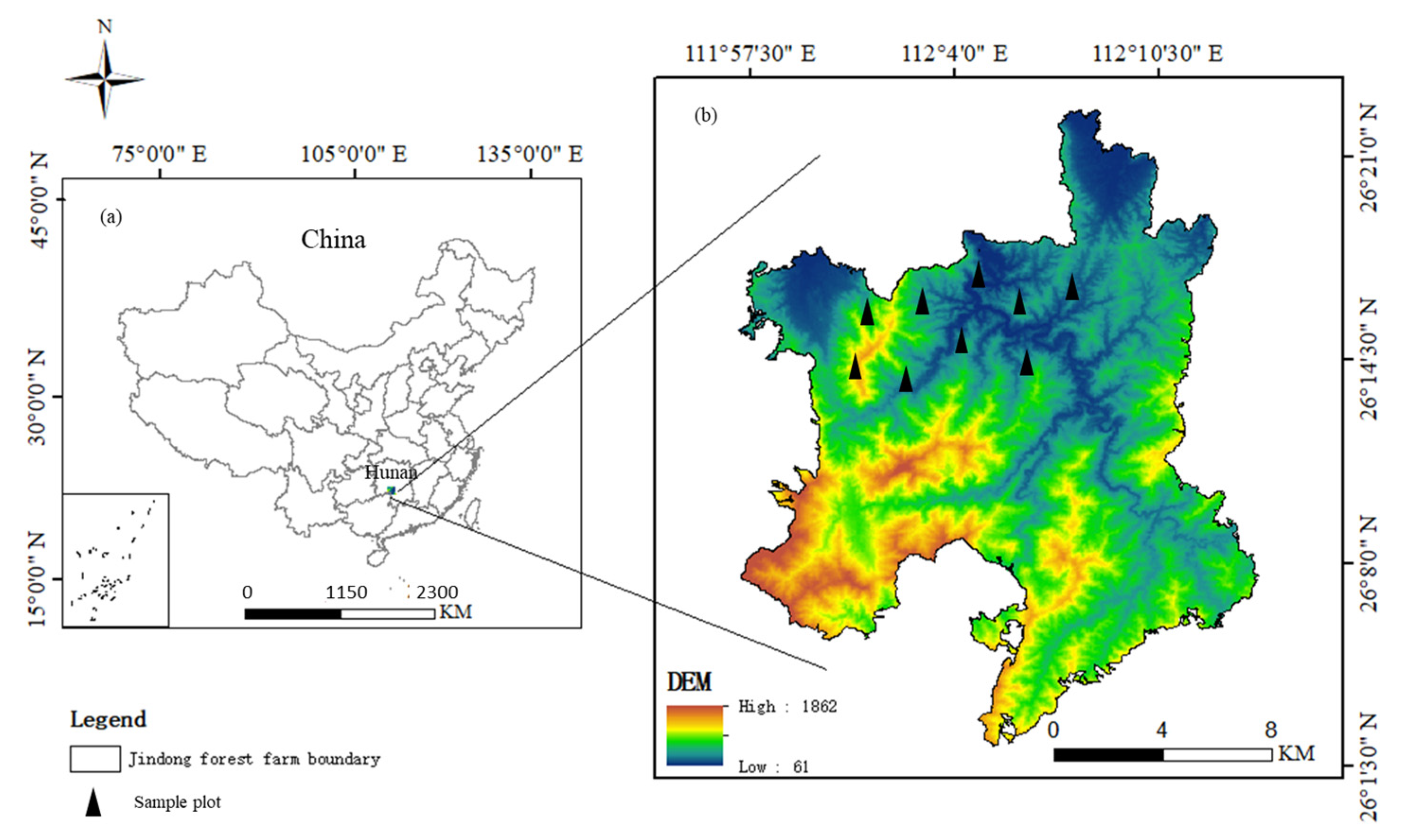
2.1. Study Area

This study was conducted at Jindong Forestry Farm, located in Yongzhou City, Hunan Province, China. The farm is situated in the upper reaches of the Xiangjiang River basin, with geographic coordinates ranging from 26°2′10″ to 26°21′37″ N and 110°53′43″ E to 112°13′37″ E. The total area of the farm is 635 square kilometers. The highest point in this region reaches an elevation of 1435 m, while the lowest point is 108 m above sea level, with an average slope of 34°. The soil of the forest farms is mainly yellow-red and yellow. It belongs to the subtropical southeast monsoon humid climate zone, with an annual average temperature of 18 °C, extreme maximum temperature of 41 °C, and extreme minimum temperature of −8 °C. The forest in this area boasts remarkable biodiversity, encompassing 135 families and 972 species of plant resources [20]. The presence of over 200 families of higher plants, comprising more than 1500 species. Among them, 98 families host 654 species of woody plants. Cunninghamia lanceolata (CL) is the main timber species in Hunan Province, and Phoebe bournei (PB) is a precious broadleaf species. Jindong Forestry Farm is the main planting area of CL and PB in the province, and the management of the CLPB mixed forest has achieved success. As a result, it has become a national demonstration site for the CLPB mixed forest model (Figure 1).

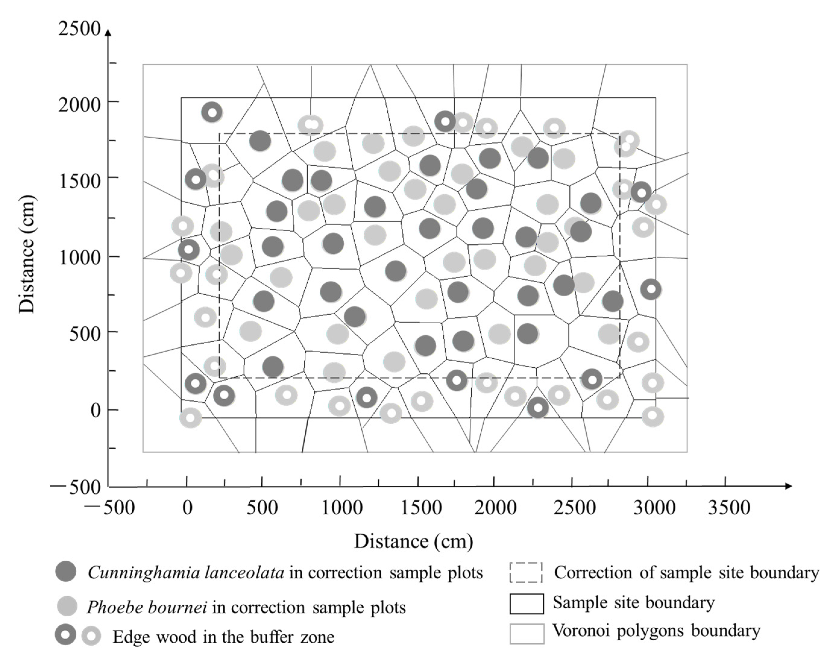
2.2. Study Design and Sampling

Nine sample plots (20 m × 30 m), including 1028 trees, were surveyed in July 2019, within a mixed forest of CLPB, and the stands in the nine plots were neatly organized and nearly uniform in age and stand conditions (

Table 1. Basic information of the sample plots.

Plot Number	Slope Aspect	Slope/Degree	Tree Number	Mean DBH /cm	Mean Height /m	Mean East–West Crown Diameter/m	Mean North–South Crown Diameter/m
1	southwestern	15	94	16.5	14.9	3.9	3.6
2	south	15	121	15.4	13.8	3.9	3.7
3	south	40	116	13.5	12.4	3.6	3.7
4	southwestern	20	125	12.9	10.1	2.1	2.6
5	south	14	98	13.5	11.8	2.5	2.8
6	south	20	126	9.6	8.5	3.1	3.3
7	southwestern	16	122	14.7	13.9	2.6	2.9
8	southwestern	15	95	10.7	9.1	2.5	2.4
9	south	20	131	13.1	12.7	3.3	3.2

). To mitigate potential edge effects, a 2 m buffer zone was implemented around the sample plot. Trees within this buffer zone were considered solely as nearest neighbors (edge woods) and were not used as reference trees (Figure 2). Trees in the buffer zone were excluded, and the remaining 637 trees were considered the object. All trees with DBH ≥ 5 cm and height ≥ 2 m in the sample plot were examined, and their DBH, tree height, X and Y coordinates, as well as the elevation and slope of the sample plot, were meticulously recorded.

2.3. Forest Spatial Structure Parameters

The spatial structure unit of a forest stand is the basic unit composed of any central wood in a forest stand and its nearest neighboring woods, which is the basis for calculating the spatial structure index and analyzing the spatial structure characteristics of a forest stand. The spatial structure unit serves as the fundamental entity for spatial structure analysis. Four neighboring trees are the four trees closest in vertical distance to the reference tree. We selected four neighboring trees proximate to the reference tree to establish this spatial structure unit [21]. In this study, the mingling degree ($M_i$), uniform angle index ($W_i$), dominance index ($U_i$), crowdedness index ($C_i$), openness index ($O_i$), and story index ($S_i$) were used to analyze the mingling status, spatial distribution pattern, size distribution, crowding degree, openness degree, and vertical stratification of the stand [22,23].

The $M_i$ describes the degree of segregation among tree species. The values of $M_i$ were divided into five intervals of 0, (0, 0.25], (0.25, 0.5], (0.5, 0.75], and (0.75, 1], corresponding to zero mixing, low mixing, moderate mixing, high mixing, and complete mixing among the stands, respectively. The $W_i$ serves as a parameter for analyzing the stand’s spatial distribution pattern, and the criteria for determining the W are that when the uniform angle mean $\overline{W}$ is [0, 0.475), the distribution pattern of the stand is uniform; when the $\overline{W}$ is in the range of [0.475, 0.517], the distribution pattern of the stand tends to be random; when the $\overline{W}$ is (0.517, 1], the distribution pattern of forest trees tends to be clumped. The $U_i$ reflects the degree of size differentiation among species, with values ranging from 0 to 1. Lower values indicate that fewer neighboring trees possess a larger DBH compared to the reference tree. The value of $U_i$ is divided into five intervals of 0, (0, 0.25], (0.25, 0.5], (0.5, 0.75], (0.75, 1], which correspond to the predominant, subdominant, intermediate, disadvantaged, and absolutely disadvantaged status of trees within the stand, respectively. The $C_i$ quantifies stand density by measuring the proportion of crown-connected reference trees among the examined nearest neighboring trees. Canopy connectivity refers to the overlap of the horizontal projections of the canopies of adjacent trees, including full or partial overlap; canopies that are just tangential or relatively independent are not considered connected. $O_i$ reflects the degree of shading experienced by the object tree due to neighboring trees, $O_i$∈(0,1], and it takes values of 0, 0.25, 0.50, 0.75, and 1 corresponding to the light transmission conditions in which the object tree is completely shaded, shaded, moderately open, open, and very open, respectively. The $S_i$ is a parameter that characterizes the vertical stratification diversity within stands, with values within the range (0, 1]. As the stand index approaches 1, the vertical stratification within the stand becomes more complex [24,25].

$$M_i=\frac{1}{n}{\displaystyle \sum _{j=1}^n{V}_{\mathrm{ij}}} v_{ij}=\left\{\begin{array}{c}1,\mathrm{if}\mathrm{neighbor}j\mathrm{is}\mathrm{not}\mathrm{the}\mathrm{same}\mathrm{species}\mathrm{as}\mathrm{reference}i\\ 0,\mathrm{otherwise}\end{array}\right.$$

(1)

$$W_i=\frac{1}{n}{\displaystyle \sum _{j=1}^n{Z}_{ij}} Z_{ij}=\left\{\begin{array}{c}1,\mathrm{if}\mathrm{the}j\mathrm{angle}\alpha \mathrm{is}\mathrm{less}\mathrm{than}\mathrm{the}\mathrm{standard}\mathrm{angle}{\alpha }_0\\ 0,\mathrm{otherwise}\end{array}\right.$$

(2)

$$U_i=\frac{1}{n}{\displaystyle \sum _{j=1}^n{k}_{ij}}{K}_{ij}=\left\{\begin{array}{c}0,\mathrm{if}\mathrm{neighbor}j\mathrm{DBH}\mathrm{is}\mathrm{smaller}\mathrm{than}\mathrm{the}\mathrm{DBH}\mathrm{of}\mathrm{reference}\mathrm{tree}i\\ 1,\mathrm{otherwise}\end{array}\right.$$

(3)

$$C_i=\frac{1}{n}{\sum }_{j=1}^n{p}_{ij}{p}_{ij}=\left\{\begin{array}{c}1,\mathrm{if}\mathrm{the}\mathrm{sum}\mathrm{of}\mathrm{crown}\mathrm{width}\mathrm{of}\mathrm{reference}i\mathrm{and}\mathrm{neighbor}j\\ \mathrm{is}\mathrm{greater}\mathrm{than}\mathrm{the}\mathrm{spacing}\mathrm{between}\mathrm{them}\\ 0,\mathrm{otherwise}\end{array}\right.$$

(4)

$$O_i=\frac{1}{n}{\sum }_{i=1}^n{t}_{ij}{t}_{ij}=\left\{\begin{array}{c}1,\mathrm{if}\mathrm{the}\mathrm{distance}\mathrm{of}\mathrm{reference}i\mathrm{and}\mathrm{neighbor}j\ge \mathrm{the}\mathrm{height}\mathrm{of}\\ \mathrm{neighbor}j\mathrm{minus}\mathrm{the}\mathrm{height}\mathrm{of}\mathrm{reference}i\\ 0,\mathrm{otherwise}\end{array}\right.$$

(5)

$$S_i=\frac{z_i}{3}\times \frac{1}{n}{\sum }_{j=1}^n{s}_{ij}{S}_{ij}=\left\{\begin{array}{c}1,\mathrm{if}\mathrm{reference}i\mathrm{with}\mathrm{neighbor}j\mathrm{belong}\mathrm{to}\mathrm{different}\\ \mathrm{layer}\\ 0,\mathrm{if}\mathrm{reference}i\mathrm{with}\mathrm{neighbor}j\mathrm{belong}\mathrm{to}\mathrm{the}\mathrm{same}\\ \mathrm{layer}\end{array}\right.$$

(6)

where, in Equations (1)–(6), n is equal to 4. In Equation (6), “$z_i$” represents the number of canopy layers in the spatial structural unit where the subject tree is located.

2.4. Coupling Method

${M_i,W}_i$, $U_i{,O_i,S}_i$ and $C_i$ are all mutually independent. Each of these indices exhibits five possible values, with the exception of $S_i$, specifically, 0.00, 0.25, 0.50, 0.75, and 1.00. In our study, we considered seven possible values for $S_i$ (0.00, 0.08, 0.17, 0.25, 0.33, 0.50, 0.67). The independence and finite nature of each index establish two essential mathematical conditions for the joint probability distribution of discrete random variables. To comprehensively describe structural heterogeneity in all facets of forest stand spatial structure, we employed multiple distributions simultaneously by combining these six variables in a flexible and appropriate manner. We calculated the values of six spatial structure indices for a total of 637 trees in nine sample plots and calculated the relative frequency of trees with the same index value for all trees. This led to the derivation of 15 binary distributions, 20 ternary distributions, 15 quadratic distributions, 6 quintic distributions, and 1 hexadecimal distribution.

2.5. Statistical Analysis

We calculate the spatial structure indices ($W_i,M_i{,U}_i{,S}_i{,C}_i{,O}_i$) for each tree using a Visual Basic program developed within EXCEL. These six parameters were combined to construct a multivariate distribution and relative frequencies were subsequently calculated. Plot boundary correction and construction of a weighted Voronoi diagram are carried out using ArcGIS 10.4. The figures were generated using R 3.4.3 software.

3. Results

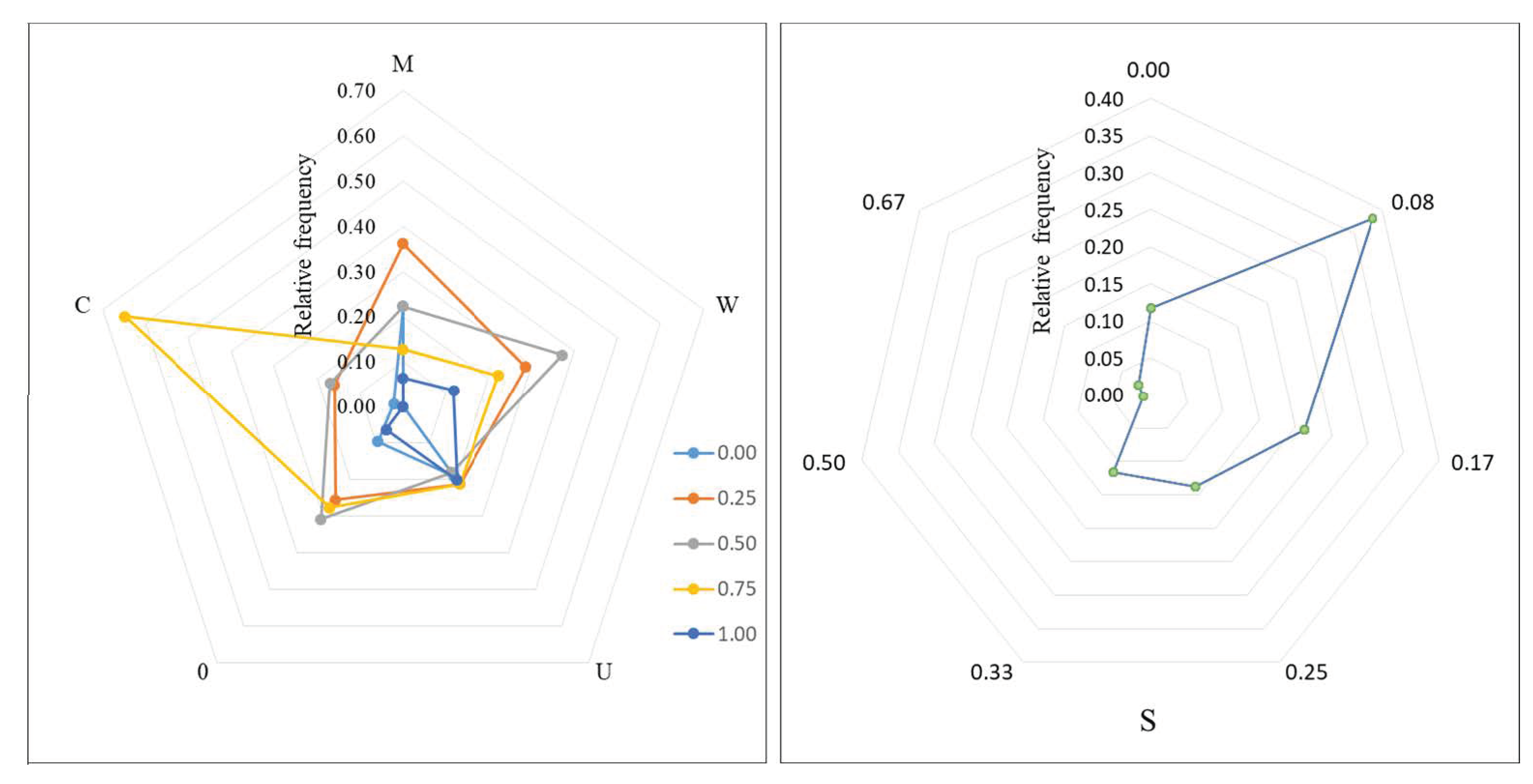
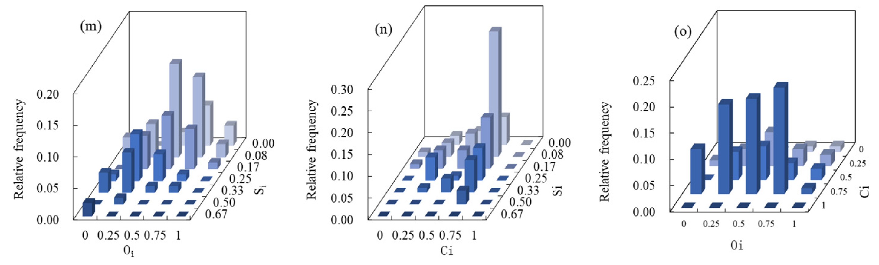
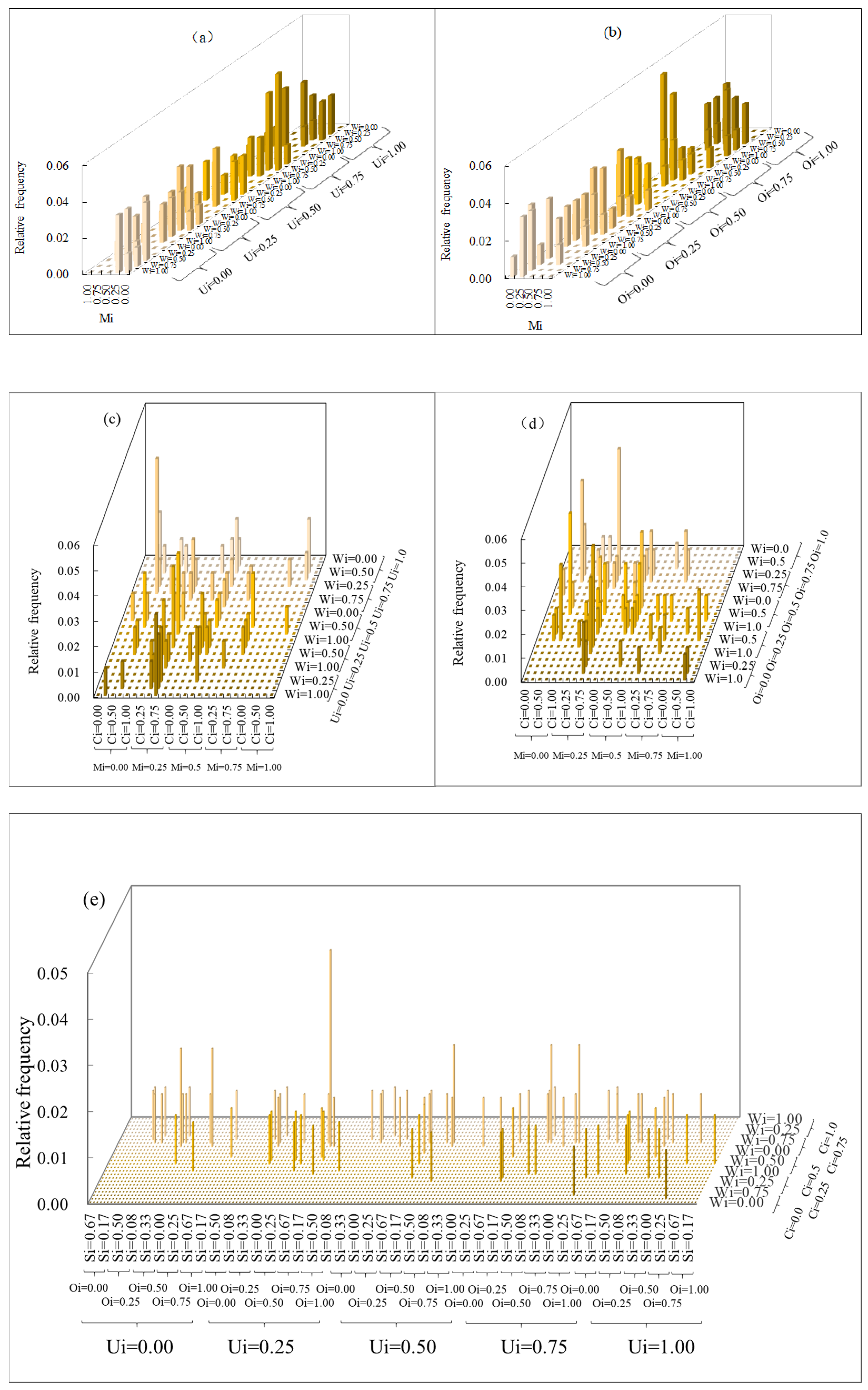
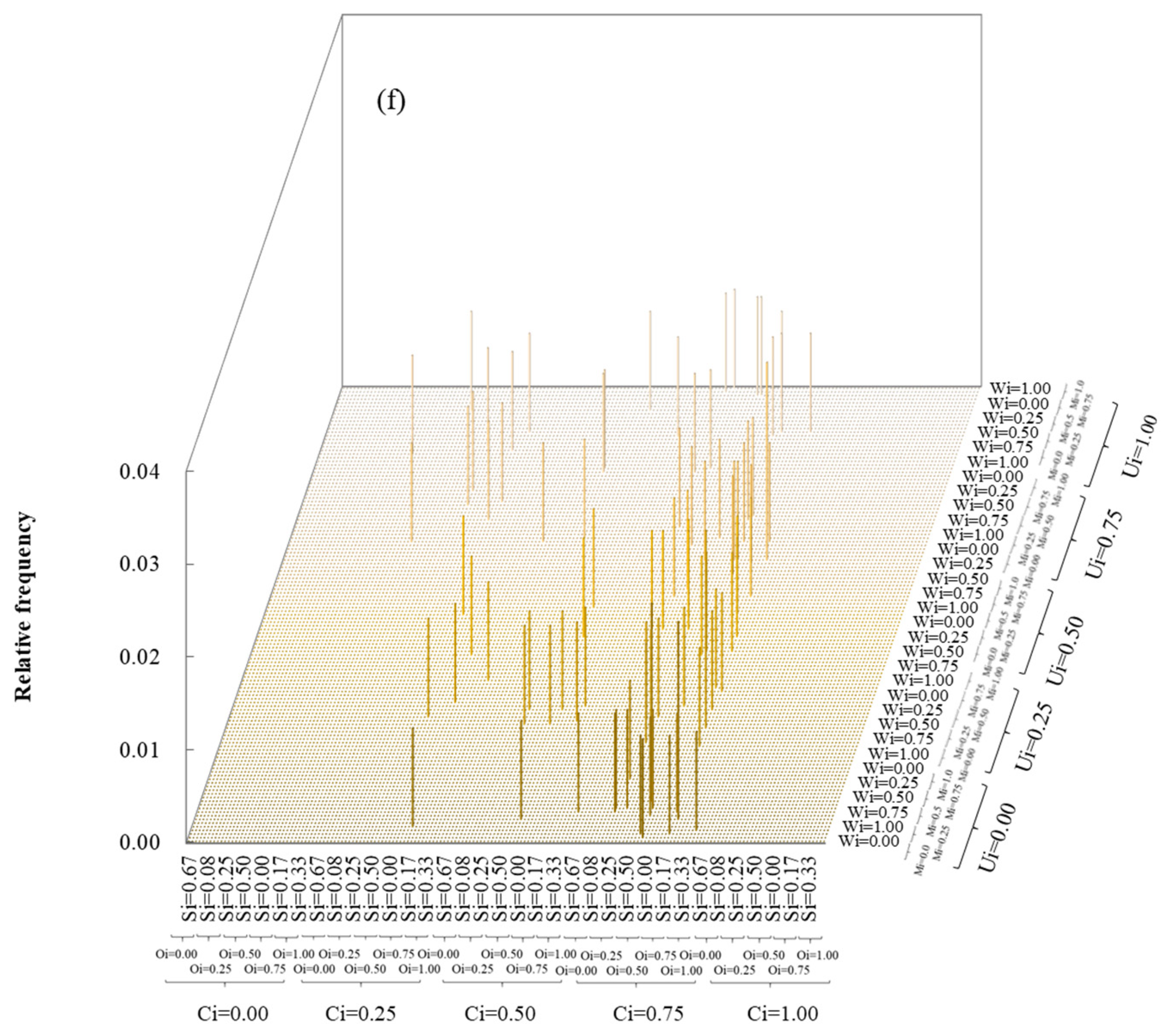
3.1. Multivariate Distribution of Spatial Structure Indices

Based on the results of spatial structure parameter calculations for 9 sample plots, it can be concluded that the degree of stand mixture was relatively low ($\overline{M}=$0.36), stand distribution pattern was clumped ($\overline{W}$= 0.54), stands were at a disadvantage in the stand ($\overline{U}$= 0.51), stand light penetration was moderately open ($\overline{O}$= 0.49), stand stratification was simple in the vertical direction ($\overline{S}$= 0.16), and the degree of stand crowding was moderate to mild ($\overline{C}$= 0.61).

The ‘M’ showed a weakly mixed distribution, with $M_i$= 0.25 being the most prevalent at 36.17% (Figure 3), followed by zero mixed and medium mixed ($M_i$ = 0.00, $M_i$ = 0.50), both occupying 22.34%. In contrast, $M_i$ = 0.75 and $M_i$ = 1.00 categories were less common, representing only 12.77% and 6.38% of the data, respectively. Regarding ‘W’ distribution, it displayed a random pattern, with $W_i$ = 0.50 being the most dominant at 37.23%, followed by a uniform distribution and a clumped distribution ($W_i$ = 0.25, $W_i$ = 0.75) with 28.72% and 22.34%. The remaining category ($W_i$ = 1.00) constituted only 11.70% of the data, while ‘uniform distribution ($W_i$ = 0.00) had no occurrences. The ‘U’ category is characterized as subdominant and inferior, with ‘$U_i$= 0.25’ and ‘$U_i$= 0.75’ being the most prevalent, both accounting for 21.28%. This is followed by the ‘inferior’ and ‘superior’ categories ($U_i$= 1.00 and $U_i$= 0.00) at 20.21% and 19.15%, respectively, while the ‘moderate’ category ($U_i$= 0.50) is less common, representing only 18.09% of the data. In the case of ‘O,’ it exhibits a moderately open distribution, with ‘$O_i$= 0.50’ being the most abundant, representing 30.85% of the observations. This is followed by the ‘open’ and ‘shaded’ categories ($O_i$= 0.75 and $O_i$= 0.25) at 27.66% and 25.53%, respectively. Conversely, the ‘completely shaded’ and ‘very open’ categories ($O_i$= 0.00 and $O_i$= 1.00) are less frequent, accounting for only 9.57% and 6.38%, respectively. The category with a ‘crowded’ level ($C_i$= 0.75) was the most prevalent, representing 64.89 % of the data. This was followed by ‘moderate’ and ‘sparse’ categories ($C_i$= 0.50 and $C_i$= 0.25), which accounted for 17.02% and 15.96%, respectively. In contrast, the ‘completely crowded’ category ($C_i$= 1.00) had no occurrences, while the ‘completely open’ category ($C_i$= 0.00) was rare, constituting only 2.13%. As for the forest layer structure (S), the ‘simple structure’ ($S_i$= 0.08) was the most abundant, comprising 38.30% of the observations. This was followed by categories $S_i$= 0.17, $S_i$= 0.25, $S_i$= 0.33, and $S_i$= 0.00, which represented 21.28%, 13.83%, 11.70%, and 11.70%, respectively. The remaining categories ($S_i$= 0.67 and $S_i$= 0.50) were less frequent, accounting for only 2.13% and 1.06%, respectively.

As the angular scale level increases, there is a tendency for frequency values at the same mixing degree to initially increase and then decrease with the rise in angular scale. In general, these values exhibit a normal distribution, with an angular scale of $W_i$ = 0.5 serving as the median axis. Trees sharing the same mixing degree are predominantly randomly distributed, particularly those with a light mixing pattern ($M_i$= 0.00, 0.25). Notably, trees with random distribution and weak mixing with other species ($W_i$= 0.50, $M_i$= 0.00) constitute 13.83% of the total tree population (Figure 4a). As the mingling degree ($M_i$) varies from 0.00 to 1.00, the frequency of subdominant trees ($U_i$) experiences an initial increase followed by a decrease, peaking near $U_i$= 0.25. This suggests that a majority of trees sharing the same mixing degree are subdominant ($U_i$= 0.25), with frequency values ranging from 3.19% to 10.64%. Furthermore, the frequency values among trees with the same mixing degree are similar across various size differentiation classes (Figure 4b). The $\mathrm{‘}M$-$O$’ bivariate distribution was predominantly concentrated in the range of $M_i$= 0.00 to $M_i$= 0.50, along with $O_i$= 0.25 to $O_i$= 0.75 (Figure 4c). The highest frequency within the ‘$C$-$M$’ bivariate distribution reached 22.34% and was centered at $M_i$= 0.25 and $C_i$= 0.75, indicating that neighboring trees exhibited mild intermixing, with overlapping crowns as the most common structural unit (Figure 4d). As the angular scale increased, the distribution frequency of trees within the same stand size differentiation class exhibited a trend of initial increase followed by a decrease (Figure 4e). Similarly, as the angular scale increased, the distribution frequency of trees within the same level of openness displayed a pattern of initial increase followed by a decrease, with $W_i$= 0.5 serving as the central axis (Figure 4f). The highest frequency in the ‘$W$-$C$’ bivariate distribution reached 26.60% at $W_i$= 0.5 and $C_i$= 0.75 (Figure 4g). The ‘$U$-$C$’ bivariate was concentrated at $C_i$= 0.75, and there were no significant differences in the frequency of trees with varying degrees of hairline differentiation (Figure 4h). Evidently, there were no significant differences in the frequency of trees with varying degrees of size differentiation within the same openness levels. Moreover, the majority of trees sharing the same size differentiation exhibited intermediate openness levels, including $M_i$ = 0.25, 0.50, and 0.75 (Figure 4i). Within the ‘$W$-$\mathrm{S}$’ bivariate distribution, the highest frequency, at 14.89%, was observed at $W_i$= 0.5 and $S_i$= 0.08 (Figure 4j). However, there was no discernible pattern in the trend of the ‘$U$-$S$’ bivariate distribution (Figure 4k). The ‘$M$-$S$’ bivariate distribution reached its highest frequency, 19.15%, at $W_i$= 0.25 and $S_i$= 0.08 (Figure 4l). When the forest index decreased, there was a gradual increase in frequency values within the same openness class as the forest index decreased (Figure 4m). For the ‘$C$-$S$’ bivariate distribution, the highest frequency, at 28.72%, was observed at $C_i$= 0.75 and $S_i$= 0.08 (Figure 4n). As the openness index increased, frequency values within the same density class exhibited an initial increase followed by a decrease, primarily concentrated at $C_i$= 0.75 and $C_i$= 0~0.75 (Figure 4o).

Within CLPB mixed forests, trees sharing the same spatial pattern and degree of dominance were typically surrounded by a larger proportion of the same species or one or two different species ($M_i$= 0.00–0.50). Notably, the most significant occurrence of identical species ($U_i$= 0.75, $W_i$= 0.50, $M_i$= 0.00) was observed in a random distribution around smaller trees, accounting for 5.32 % of the total (Figure 5a). The ternary distribution of M-W-O exhibited a trend similar to that of M-W-U (Figure 5b). The quadratic distribution pattern (Figure 5c, d) revealed a significant proportion of trees sharing the same distribution pattern, characterized by moderate openness and mingling ($M_i$= 0.25, 0.50). Among the various combinations, $M_i$= 0.00, $W_i$= 0.50, $C_i$= 0.75, $U_i$= 0.75 (Figure 5c) exhibited a notably high frequency, accounting for 5.32% of the total. Similarly, $M_i$= 0.25, $W_i$= 0.25, $C_i$= 0.75, $O_i$= 0.75 (Figure 5d) also represented 5.32% of the total frequency. This observation suggests that the stand exhibited a light mixing of tree species, had a more open canopy, and featured random tree distribution, particularly with trees of below-average diameter at breast height and a continuous dense canopy. The quintic distribution (Figure 5e) revealed that the combination $W_i$= 0.25, $C_i$= 0.75, $S_i$= 0.08, $O_i$= 0.75, $U_i$= 0.25 had the highest percentage at 4.26%. This indicates that trees within the stand, featuring a stand diameter at breast height (DBH) lower than the mean, a simple stand structure, and a continuous dense canopy, exhibited a light mixing pattern. Additionally, they were more open, arranged in a regular or random distribution. For most of the five-dimensional variables of forest trees within the stand, frequencies ranged from 0% to 2.13%, with a few extending from 2.13% to 3.19%.

The hexadecimal distribution characterizes the stand structure in six simultaneous ways, and within the combination presented in Figure 5f, the joint distribution of hexadecimal variables attains the highest frequency at 2.13%. In particular, this frequency is associated with the following combinations: $U_i$= 0.00, $C_i$= 0.75, $M_i$= 0.25, $O_i$= 0.75, $W_i$= 0.25, $S_i$= 0.00; $U_i$= 0.00, $C_i$= 0.75, $M_i$= 0.50, $O_i$= 0.50, $W_i$= 0.25, $S_i$= 0.17; $U_i$= 0.25, $C_i$= 0.75, $M_i$= 0.25, $O_i$= 0.75, $W_i$= 0.25, $S_i$= 0.08; $U_i$= 0.75, $C_i$= 0.75, $M_i$= 0.00, $O_i$= 0.75, $W_i$= 0.50, $S_i$= 0.00. In stands characterized by object trees with a diameter at breast height (DBH) smaller than neighboring trees and featuring simple canopy structures that touch each other but are relatively open, a light mingling pattern prevails, with trees arranged in a regular or random distribution. The next most significant distribution occurs at 1.06 % and represents the highest frequency in this context.

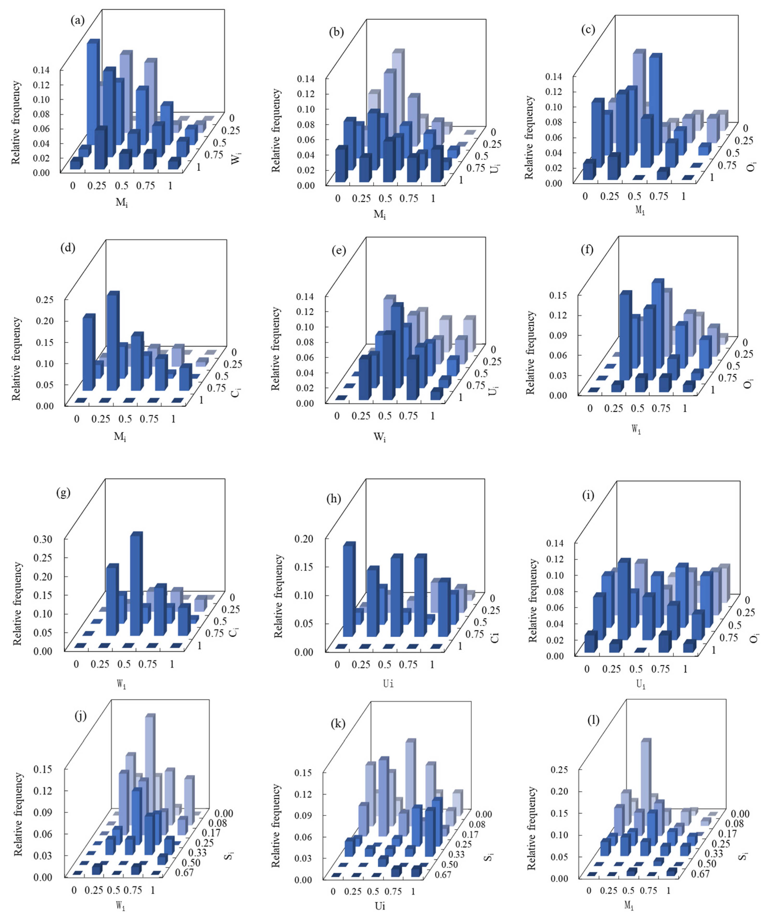
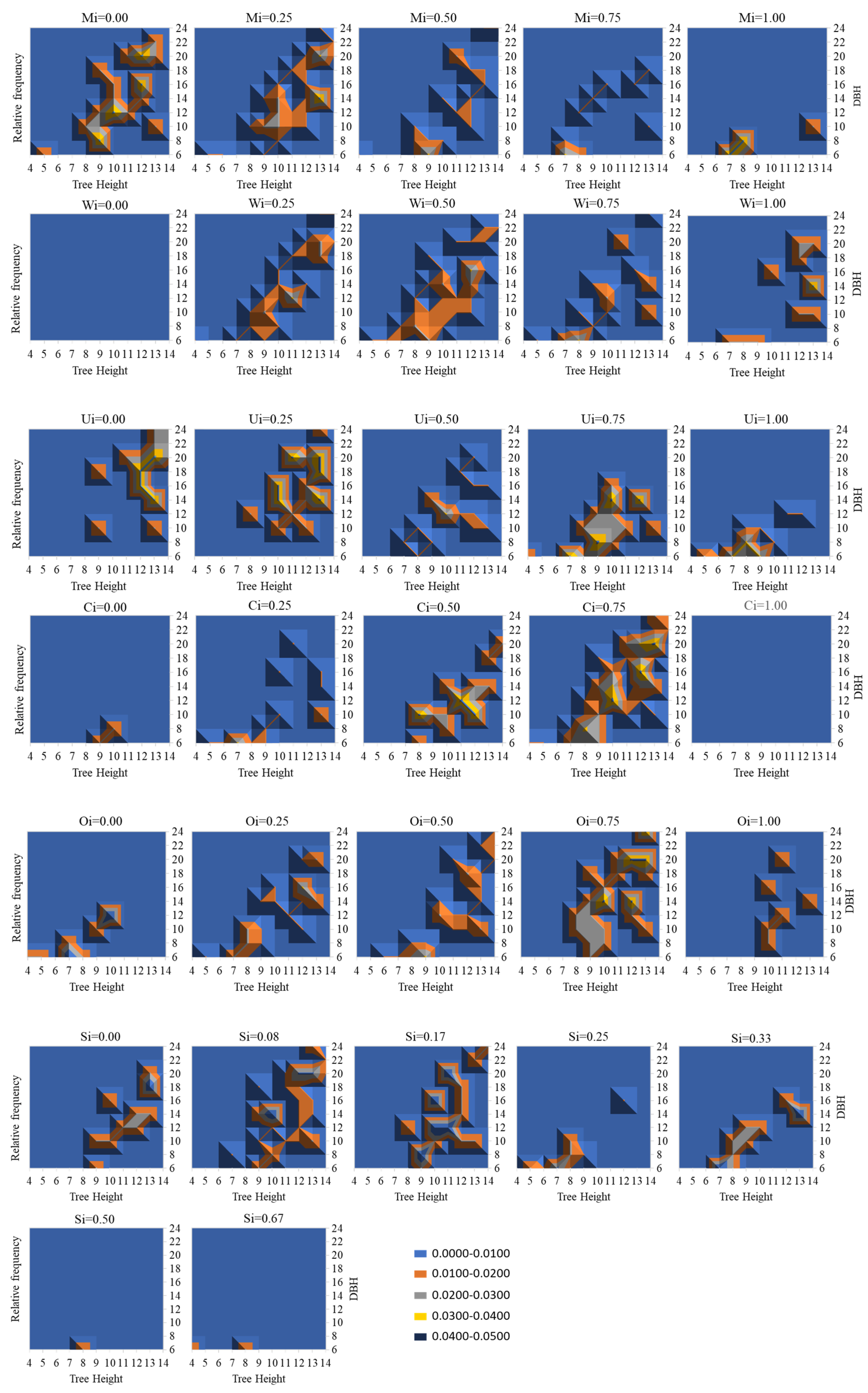
3.2. Coupling of Spatial Structure Indices and Tree Size

In CLPB mixed forests, we selected 2 cm as the step size for DBH and 1 m for tree height length, which were then rectified using the upper exclusion method. The DBH and tree height data were combined with the spatial indices M, W, U, C, O, and S, resulting in the generation of DBH-H-spatial structure indices (Figure 6). The highest joint frequency observed between M, DBH, and tree height reached 4.26%, occurring at a DBH of 14 cm and a tree height of 13 m ($M_i$= 0.25). The relative frequency values were predominantly distributed within the DBH range of 6–20 cm and a tree height range of 7–13 m. For W, the highest joint frequency with DBH and tree height reached 3.19% at a DBH of 12 cm and a tree height of 11 m ($W_i$= 0.25). The primary range of distribution for relative frequency values was similar to that of M. In the case of U, the main range of distribution for joint relative frequency values was similar to that of M and W. The highest joint frequency was observed between C and DBH, and the tree height reached 4.26% and was distributed at DBH = 12, H = 10m; DBH = 16, H = 12m; and DBH = 20, H = 13m, characterizing more crowded stands ($C_i$= 0.75). The ‘O’ displayed the highest joint frequency with DBH and tree height at 3.19%, distributed at DBH = 6, H = 9m and DBH = 16, H = 12m and stands with shaded or moderately open conditions ($O_i$= 0.25, 0.50). The ‘S’ achieved the highest joint frequency with DBH and tree height at 4.26%, occurring at DBH = 14, H = 10 m, where the stand structure was simpler ($S_i$= 0.08). This was followed by 3.19% at DBH = 6, H = 7 m and at DBH = 20, H = 12 and 13 m, where the stand structure was simpler ($S_i$= 0.25).

4. Discussion

4.1. The Superiority of the Six-Variable Distribution Method Compared to the Univariate Method

The zero-variate distribution characterizes the overall forest structure by employing a single mean value, while the univariate distribution assesses individual structural attributes in isolation, examining the relative proportions of trees across various possible values for each spatial attribute. Analyzing a single spatial structural parameter of a forest stand in isolation can result in one-sided conclusions [26]. For example, when assessing tree distribution patterns without considering factors such as mingling degree and size differentiation among trees, challenges related to species allocation and inter-tree competitive growth may emerge [27]. Therefore, it is crucial to analyze specific structural parameters while concurrently considering other relevant structural attributes.

Multivariate distributions encompass various facets of forest structure by simultaneously depicting the relative frequencies of N combinations of structural parameters, enabling a precise quantification of diverse structural characteristics [28]. Transitioning from univariate distribution to N-variate distribution, this spatial analytic geometry progressively interprets structures, advancing from points to lines, surfaces, cubes, and hyperloids [29,30,31]. Consequently, multivariate distribution adeptly integrates multiple spatial structural parameters to construct an N-variate distribution, addressing the need for a comprehensive structural interpretation of real forest stands [32]. This multivariate distribution of spatial structural parameters for forest stands offers an intuitive representation of distribution patterns and quantitative attributes of joint structural parameters [33,34,35].

The hexadecimal distribution of the M-W-U-C-O-S spatial structural parameters, as introduced in this study, encompasses 5 × 5 × 5 × 5 × 5 × 5 = 15,625 distinctive structural combinations. This comprehensive framework facilitates a simultaneous and intricate representation of forest spatial structure from six distinct perspectives. In contrast to univariate and null-variate distributions, the hexadecadal distribution provides 5, 25, 125, 625, 3125, and 15,625 times more detailed information, respectively. These multivariate distributions offer a comprehensive and systematic quantitative portrayal of forest structure across multiple levels of resolution [36,37]. Traditionally, previous investigations have often examined forest spatial characteristics from singular viewpoints [38,39] or, at most, from four aspects [19], thereby lacking a comprehensive and systematic understanding of forest structural attributes. The six-dimensional distribution concurrently elucidates spatial patterns, species diversity, size differentiation, forest stratification, crowding, and openness. This advances our comprehension of structural characteristics, surpassing earlier studies that relied on other distributions or conventional methods, which could only reveal forest structure at limited levels of resolution.

4.2. Relationship between Forest Spatial Structure and Tree Size

Good spatial structure is often associated with higher tree growth rates; in contrast, forests with poor structures exhibit lower growth performances. There is a close and intricate relationship between forest spatial structure and tree growth. Trees in the forest rely on resources such as light, water, nutrients, and space, and the spatial structure directly influences the distribution and availability of these resources. In densely packed forest stands, tree competition for limited resources can intensify, restricting the growth of individual trees. Conversely, in more open forest stands, resources are more abundant, and competition among trees is reduced, thereby promoting their growth [40]. The canopy structure and arrangement of trees in a forest play a crucial role in the distribution and utilization of light. Tall and dense canopies may restrict the penetration of light to the understory vegetation and lower trees, which can affect their photosynthesis and growth. Reduced light levels lead to a slowdown in tree growth [41]. The relationship between the spatial structural parameters of forests and tree growth is a critical research topic in the fields of ecology and forestry. Different spatial structures can influence tree growth. Studies have shown that high levels of tree species diversity contribute to enhanced forest growth. Mixed tree species can share resources, reduce competition, improve light utilization efficiency, and provide more ecological niches, thereby promoting tree growth [42]. Lower size ratios may favor the growth of smaller trees as they are not obstructed by larger ones [43]. Research has indicated a positive correlation between openness and tree growth [44]. Higher density can lead to increased competition among larger trees for limited resources; therefore, moderate tree density is often more favorable for tree growth [45]. Investigating these parameters is essential for the effective management and conservation of forest ecosystems, enabling sustainable forest management and the maintenance of ecological balance.

4.3. The Role of the N-Variable Distribution Method in Forest Structure Adjustment

These six spatial variables serve as valuable tools for describing, comparing, and assessing forest structure, including its transformations resulting from harvesting activities [46]. Consequently, the flexible combinations of structural parameters, exemplified by N-variable distributions, hold significant promise for guiding forest management [47]. This approach is especially pertinent in the context of directing forest thinning [48,49] and optimizing forest utilization. Multivariate distributions offer insights across varying resolution levels and from diverse perspectives [50]. By analyzing the frequency distribution of tree attributes pre-harvest, forestry professionals gain enhanced abilities to assess neighborhood competition, make informed decisions regarding tree selection for harvesting, and evaluate alterations in forest structure by comparing structural distributions before and after harvests. In finer detail, forest structuring often thrives when it involves mixed, randomly distributed trees featuring reasonable degrees of dominance and crowding—a concept that has garnered recognition in recent studies [51,52]. The multivariate distribution of forest structure serves as an effective guide for forest selection [53]. In cases where all six indicators exhibit poor values, prioritizing the felling of the stand is the initial course of action, followed by the removal of trees with five poor indicators, and so forth. Trees exhibiting inadequacy in only one variable are the last to be considered for felling. This multivariate distribution empowers us to fine-tune forest structure with precision.

Forest structure is a central concern in forestry, as a well-structured forest offers optimal space and growth conditions for individual trees within a stand [54]. Conversely, suboptimal structures, such as clustered distributions, can lead to incremental losses [55]. There is a growing recognition that the spatial arrangements of tree locations and sizes within a stand can significantly impact the overall value generated via the forest [56,57,58]. Effective forest management should revolve around the harmonious relationship between stand structure and function, aiming to optimize stand structure by adjusting its parameters to fully harness the manifold functions of the forest [59,60]. The six-element distribution introduced in this study provides comprehensive insights into horizontal forest structure, facilitating the reduction in disparities between simulated and ideal forest structures. Informed by the insights gleaned from multivariate distribution analyses of spatial structure, structural adjustments can be implemented for the CLPB mixed forest. These adjustments involve adopting management strategies that prioritize the removal of inferior specimens while preserving superior ones, promoting the retention of broadleaved trees over needled ones, and introducing high-quality native broadleaf species [61]. This approach aims to enhance the stand mixture while considering the stand’s distribution pattern, ultimately aligning the forest stand’s structure with a state of random distribution. Such efforts bridge the gap between the actual forest structure and the ideal one, ultimately promoting the health, stability, and sustainable development of forest stands.

4.4. Limitations

The primary achievement of this study lies in the development of a novel spatial structure analysis approach known as the hexadecimal distribution method. This method was applied to analyze the spatial structure of mixed coniferous and broadleaf forests in the southern regions of the country, specifically at the sample plot scale. There is significant potential for expanding the scope of this study to encompass larger geographical areas. Future research can delve into hexadecimal distribution characteristics at a regional scale, offering a broader examination of spatial structures in forest stands.

While this study primarily focused on mixed coniferous and broadleaf forests, it sets the stage for the analysis of other forest stand types in subsequent research. Moreover, comparisons and in-depth analyses can be conducted between similar forest stands in both northern and southern regions. These endeavors hold the promise of providing valuable theoretical insights into the structural analysis of forests across diverse regions and forest stand types.

5. Conclusions

This study highlights the comprehensive potential of the six-variable distribution method in assessing forest spatial structure. In comparison to univariate distributions, the six-variable distribution offers a more extensive multidimensional perspective, encompassing a staggering 15,625 distinct structural combinations (5 × 5 × 5 × 5 × 5 × 5), enabling an in-depth analysis of forest spatial structure from multiple angles. Furthermore, we found that forest structures characterized by a slight tree mixing ($M_i$= 0.25), random distribution ($W_i$= 0.5), simple canopy structure ($S_i$= 0.08, 0.25), substantial tree contact ($C_i$= 0.75), but relatively open ($O_i$= 0.5) and moderate suitability ($U_i$= 0.5) exert a positive influence on tree growth. Furthermore, the six-variable distribution method can serve as an effective guiding approach for optimizing forest structure. If all six indicator values are poor, the priority should be to first fall the trees with the lowest values in all indicators, followed by trees with poor values in five indicators, and so on. The N-variable distribution analysis method is a potent tool for assessing forest structure and guiding the optimization of forest structural elements.

References

1. Ehbrecht, M.; Seidel, D.; Annighöfer, P.; Kreft, H.; Köhler, M.; Zemp, D.C.; Puettmann, K.; Nilus, R.; Babweteera, F.; Willim, K.; et al. Global patterns and climatic controls of forest structural complexity. Nat. Commun. 2021, 12, 519. [Google Scholar] [CrossRef] [PubMed]
2. McElhinny, C.; Gibbons, P.; Brack, C.; Bauhus, J. Forest and woodland stand structural complexity: Its definition and measurement. For. Ecol. Manag. 2005, 218, 1–24. [Google Scholar] [CrossRef]
3. Lindenmayer, D.B.; Franklin, J.F.; Fischer, J. General management principles and a checklist of strategies to guide forest biodiversity conservation. Biol. Conserv. 2006, 131, 433–445. [Google Scholar] [CrossRef]
4. Gustafsson, L.; Baker, S.C.; Bauhus, J.; Beese, W.J.; Brodie, A.; Kouki, J.; Lindenmayer, D.B.; Lõhmus, A.; Pastur, G.M.; Messier, C.; et al. Retention Forestry to Maintain Multifunctional Forests: A World Perspective. Bioscience 2012, 62, 633–645. [Google Scholar] [CrossRef]
5. Chirici, G.; McRoberts, R.E.; Winter, S.; Barbati, A.; Brändli, U.B.; Abegg, M.; Beranova, J.; Rondeux, J.; Bertini, R.; Alberdi Asensio, I.; et al. National Forest Inventory Contributions to Forest Biodiversity Monitoring. For. Ecol. Manag. 2016, 356, 12–26. [Google Scholar] [CrossRef]
6. Coates, K.D.; Haeussler, S. The Use of Stand Structural Attributes in Understanding and Managing Coast Interior Cedar-Hemlock Forests. For. Ecol. Manag. 2003, 172, 229–244. [Google Scholar]
7. MacFarlane, D.W.; MacFarlane, D.M.; Keith, D.A. Towards consistent classification of structural forest attributes. For. Ecol. Manag. 2017, 394, 11–20. [Google Scholar]
8. Lutz, J.A.; Larson, A.J.; Freund, J.A.; Swanson, M.E.; Bible, K.J. The Importance of Large-Diameter Trees to Forest Structural Heterogeneity. PLoS ONE 2012, 7, e36398. [Google Scholar] [CrossRef]
9. Parresol, B.R. Assessing Tree and Stand Biomass: A Review with Examples and Critical Comparisons. For. Sci. 1999, 45, 573–593. [Google Scholar]
10. Hui, G.Y.; Hu, Y.B.; Zhao, Z.H. Research Progress in Structured Forest Management. For. Sci. Res. 2018, 31, 85–93. [Google Scholar] [CrossRef]
11. Bélisle, C.; Desrochers, A. The Influence of Forest Stand Structure on Bird Communities in Boreal Forests of Quebec: An Assessment at Two Spatial Scales. Can. J. For. Res. 2002, 32, 388–399. [Google Scholar]
12. Hui, G.; Gu, H. Enhancing forest diversity by combining different thinning approaches: A case study in northeastern China. For. Ecol. Manag. 2017, 389, 94–102. [Google Scholar]
13. Pukkala, T.; Kolström, T. Assessment of structural diversity in uneven-sized stands. For. Ecol. Manag. 2000, 135, 147–155. [Google Scholar]
14. Zhang, J.; Kang, S.; Zhang, Y. Spatio-temporal variations of structural diversity of Picea crassifolia forests in the Qilian Mountains, northwestern China. Ecol. Res. 2010, 25, 425–436. [Google Scholar]
15. Gadow, K.V.; Hui, G.Y. Modeling Forest Development; Springer: Berlin/Heidelberg, Germany, 1999. [Google Scholar]
16. Lefsky, M.A.; Cohen, W.B.; Harding, D.J.; Parker, G.G.; Shugart, H.H.; Gower, S.T. Lidar Remote Sensing for Ecosystem Studies. BioScience 2002, 52, 19–30. [Google Scholar] [CrossRef]
17. Kint, V.; Clarke, N.; Vesterdal, L. Quantifying fine-root biomass in Scots pine and Norway spruce stands using fine-root diameter and biomass equations. Tree Physiol. 2003, 23, 885–891. [Google Scholar]
18. Li, Y.; Ye, S.; Hui, G.; Hu, Y.; Zhao, Z. Spatial structure of timber harvested according to structure-based forest management. For. Ecol. Manag. 2014, 322, 106–116. [Google Scholar] [CrossRef]
19. Zhang, G.; Hui, G.; Zhang, G.; Zhao, Z.; Hu, Y. Telescope method for characterizing the spatial structure of a pine-oak mixed forest in the Xiaolong Mountains, China. Scand. J. For. Res. 2019, 34, 751–762. [Google Scholar] [CrossRef]
20. Howard, J.L.; Gagne, M.; Morin, A.J.S.; Forest, J. Using Bifactor Exploratory Structural Equation Modeling to Test for a Continuum Structure of Motivation. Management 2016, 44, 2638–2664. [Google Scholar] [CrossRef]
21. Perry, D.A.; Lotan, J.E. A framework for the development of forest spatial patterns. For. Sci. 1975, 21, 370–380. [Google Scholar]
22. Aguirre, O.; Hui, G.; von Gadow, K.; Jiménez, J. An analysis of spatial forest structure using neighbourhood-based variables. For. Ecol. Manag. 2003, 183, 137–145. [Google Scholar] [CrossRef]
23. Hui, G.Y.; Hu, Y.B. Measuring species spatial isolation in mixed forests. For. Res. 2001, 14, 23–27. [Google Scholar]
24. Hui, G.Y.; Zhao, Z.H.; Hu, Y.B.; Zhang, G.Q.; Cheng, S.P.; Xu, X.F. Comprehensive evaluation of forest stand spatial structure based on the mean value of structural parameters. For. Res. 2023, 36, 12–21. [Google Scholar] [CrossRef]
25. Hui, G.Y.; Gadow, K.V.; Zhao, Z.H.; Hu, Y.B.; Xu, H.; Li, Y.F.; Zhang, L.J.; Zhang, G.Q.; Liu, W.Z.; Yuan, S.Y. Principles of Structure-Based Forest Management; China Forestry Press: Beijing, China, 2016; Volume 6. [Google Scholar]
26. Zhu, J.; Liu, S.; Wu, F.; Liu, W. Spatial Structure and Allometric Growth of Major Tree Species in a Subtropical Evergreen Broad-Leaved Forest. PLoS ONE 2016, 11, e0155275. [Google Scholar]
27. Qian, H.; Zhang, J.; Wu, Z.; Yin, L.; Li, H. Incorporating species composition into models for stand volume using spatial linear models. For. Ecol. Manag. 2014, 328, 38–44. [Google Scholar]
28. Zhang, L.; Liang, H.; Xu, M. Spatial distributions and correlations of forest structure, composition, and soil nutrients along an altitudinal gradient in a subtropical evergreen broadleaved forest. For. Ecol. Manag. 2018, 418, 41–48. [Google Scholar]
29. Fortin, M.J.; Dale, M. Spatial Analysis: A Guide for Ecologists; Cambridge University Press: Cambridge, UK, 2005. [Google Scholar]
30. Turner, W.; Rondinini, C.; Pettorelli, N.; Mora, B.; Leidner, A.K.; Szantoi, Z.; Chauvenet, A. Free and open-access satellite data are key to biodiversity conservation. Biol. Conserv. 2015, 182, 173–176. [Google Scholar] [CrossRef]
31. Levin, N.; Lechner, A.M.; Brown, G.; Mörtberg, U.M.; Mörtberg, M.; Lechner, A.M. A review of airborne LiDAR applications for 3D modelling and analysis of forests. Remote Sens. 2017, 9, 1070. [Google Scholar]
32. He, H.S.; Shang, B.Z.; Crow, T.R.; Gustafson, E.J.; Shifley, S.R.; Fraser, J.S. Simulating forest fuel and fire risk dynamics across landscapes—LANDIS fuel module design. Ecol. Model. 2007, 201, 675–690. [Google Scholar] [CrossRef]
33. Wiegand, T.; Moloney, K.A.; Naves, J. Using process-based models to simulate tree population dynamics in monodominant tropical forests. Ecology 1999, 80, 1214–1224. [Google Scholar]
34. Pélissier, R.; Goreaud, F. A practical approach to the study of spatial structure in simple cases of heterogeneous vegetation. J. Veg. Sci. 2001, 12, 99–108. [Google Scholar] [CrossRef]
35. Li, Y.; Lei, X.; Ma, S. Analysis of forest structure using remote sensing data: A review. For. Ecol. Manag. 2020, 458, 117762. [Google Scholar]
36. Pommerenig, J.; Stoyan, D. Optimizing spatial forest structure under habitat constraints. Environ. Ecol. Stat. 2008, 15, 69–82. [Google Scholar]
37. Packard, K.C.; Radosevich, S.R. Relating vegetation and environmental gradients through quantile regression. For. Ecol. Manag. 2001, 154, 347–359. [Google Scholar]
38. Perry, D.A.; Amaranthus, M.P. The role of spatial processes in canopy dynamics. Can. J. For. Res. 2006, 36, 243–252. [Google Scholar]
39. Keenan, R.J.; Reams, G.A.; Achard, F.; de Freitas, J.V.; Grainger, A.; Lindquist, E. Dynamics of global forest area: Results from the FAO Global Forest Resources Assessment 2015. For. Ecol. Manag. 2015, 352, 9–20. [Google Scholar] [CrossRef]
40. Kobe, R.K. Sapling growth as a function of light and landscape-level variation in soil water and foliar nitrogen in northern Michigan. Oecologia 2006, 147, 119–133. [Google Scholar] [CrossRef] [PubMed]
41. Canham, C.D.; Finzi, A.C. Disentangling changes in the spectral reflectance of forest canopy and understory due to natural and anthropogenic effects. Remote Sens. Environ. 2013, 132, 51–57. [Google Scholar]
42. Paquette, A.; Messier, C. The effect of biodiversity on tree productivity: From temperate to boreal forests. Glob. Ecol. Biogeogr. 2011, 20, 170–180. [Google Scholar] [CrossRef]
43. Mladenoff, D.J.; Stearns, F. Eastern hemlock regeneration and deer browsing in the northern great lakes region: A re-examination and model simulation. Conserv. Biol. 1993, 7, 889–900. [Google Scholar] [CrossRef]
44. Canham, C.D.; Finzi, A.C.; Pacala, S.W.; Burbank, D.H. Causes and consequences of resource heterogeneity in forests: Interspecific variation in light transmission by canopy trees. Can. J. For. Res. 1994, 24, 337–349. [Google Scholar] [CrossRef]
45. Pacala, S.W.; Deutschman, D.H. Details that matter: The spatial distribution of individual trees maintains forest ecosystem function. Oikos 1995, 74, 357–365. [Google Scholar] [CrossRef]
46. Pommerening, A.; Stoyan, D. Edge-correction needs in estimating indices of spatial forest structure. Can. J. For. Res. 2008, 38, 878–889. [Google Scholar] [CrossRef]
47. Li, Y.; Weiskittel, A.R. Multivariate analysis of forest structure and composition: A systematic review and synthesis. For. Ecol. Manag. 2018, 427, 309–318. [Google Scholar]
48. Gadow, K.V.; Hui, G.Y. Modeling Forest Development; Academic Press: Cambridge, MA, USA, 2001. [Google Scholar]
49. Li, H.; Lei, X.; Tang, J. Optimizing forest structure through spatially explicit simulation and multivariate analysis of forest attributes in Northeast China. For. Ecol. Manag. 2018, 424, 409–418. [Google Scholar]
50. Pretzsch, H. Forest Dynamics, Growth, and Yield: From Measurement to Model; Springer Science Business Media: Berlin/Heidelberg, Germany, 2009. [Google Scholar]
51. Pukkala, T.; Kurttila, M.; Mehtätalo, L. A method for integrating stand growth models and harvest scheduling models. Eur. J. For. Res. 2009, 128, 1–11. [Google Scholar]
52. Temesgen, H.; Monleon, V.J. Characterizing crown structure in old-growth and mature conifer stands using terrestrial lidar data and a structural clustering algorithm. Can. J. For. Res. 2015, 45, 199–208. [Google Scholar]
53. Li, S.; Fang, X.; Chen, J.; Li, L.; Gu, X.; Liu, Z.; Zhang, S. Effects of different degrees of anthropogenic disturbance on biomass and spatial distribution in Subtropical forests in Central Southern China. Acta Ecol. Sin. 2018, 38, 6111–6124. [Google Scholar] [CrossRef]
54. Spies, T.A.; Turner, W. Dynamic forest mosaics. In Forest Landscape Ecology: Transferring Knowledge to Practice; McDonnell, M.J., Pickett, S.T.A., Eds.; Springer: Berlin/Heidelberg, Germany, 1999; pp. 155–171. [Google Scholar]
55. Pretzsch, H.; Schütze, G. Transgressive overyielding in mixed compared with pure stands of Norway spruce and European beech in Central Europe: Evidence on stand level and explanation on individual tree level. Eur. J. For. Res. 2009, 128, 183–204. [Google Scholar] [CrossRef]
56. Liang, J.; Buongiorno, J.; Monserud, R.A.; Kruger, E.L. Effects of diversity of tree species and size on forest basal area growth, recruitment, and mortality. For. Ecol. Manag. 2007, 243, 116–127. [Google Scholar] [CrossRef]
57. Reed, D.D.; Jones, D.A.; Schuler, T.M. Economic return on long-term forest productivity: A synthesis of results from 35 years of experimental management on 50 northern hardwood stands. For. Sci. 2009, 55, 93–107. [Google Scholar]
58. Buongiorno, J.; Peyron, J.L.; Houllier, F.; Bruciamacchie, M. A stand-growth model for even-aged stands of maritime pine (Pinus pinaster Ait.) in Mediterranean areas of France. For. Ecol. Manag. 2010, 259, 234–248. [Google Scholar]
59. Kelty, M.J. The role of species mixtures in plantation forestry. For. Ecol. Manag. 2006, 233, 195–204. [Google Scholar] [CrossRef]
60. Aubinet, M.; Chermanne, B.; Vandenhaute, M.; Longdoz, B.; Yernaux, M.; Laitat, E. Long term carbon dioxide exchange above a mixed forest in the Belgian Ardennes. Agric. For. Meteorol. 2001, 108, 293–315. [Google Scholar] [CrossRef]
61. Vepakomma, U.; Pukkala, T. Optimal management of teak plantations in India: A spatial approach. For. Ecol. Manag. 2016, 360, 132–141. [Google Scholar]
Figure 1. Location of the study site ((a) is the map of China, and (b) is the topographical map of Jindong Forest Farm).
Forests 14 02228 g001
Figure 2. Weighted Voronoi polygons after edge correction based on tree location point data (the points are trees, solid points represent trees within the corrected sample plots, and hollow points represent trees in the edge sample plots).
Forests 14 02228 g002
Figure 3. The distribution of the mean spatial structure parameters (M is the mingling degree, W is uniform angle index, U is dominance index, C is crowdedness index, O is openness index, and S is story index).
Forests 14 02228 g003
Figure 4. The binary distribution of spatial structure parameters of tree stands (M is the mingling degree, W is uniform angle index, U is dominance index, C is crowdedness index, O is openness index, and S is story index. (ao) are the binary distribution of M-W, the binary distribution of M-U, …, the binary distribution of O-C.
Forests 14 02228 g004aForests 14 02228 g004b
Figure 5. The N-variable distributions of spatial structure parameters ((a,b): ternary distribution, (c,d): quadratic distribution, (e): quintic distribution, (f): hexadecimal distribution. M is the mingling degree, W is uniform angle index, U is dominance index, C is crowdedness index, O is openness index, and S is story index).
Forests 14 02228 g005aForests 14 02228 g005b
Figure 6. Joint distribution of trail-tree advanced and spatial structural parameters.
Forests 14 02228 g006