A Novel Two-Phase Approach to Forest Harvesting Optimization Using Cable Logging

Abstract

Timber extraction is a vital process in forest harvesting, particularly in areas with high slopes where timber harvesting methods are not feasible. In such cases, logging towers employing extraction cables are often the most effective solution. This intricate task involves several phases, with the installation of the tower being one of the most critical. It significantly influences the performance and feasibility of timber extraction. Another crucial phase involves strategically positioning logging lines to minimize the installation time while maximizing the load capacity efficiency. This article presents an integer programming mathematical model for determining the optimal positioning of yarders conditioned to logging lines, the timber logging time, and the logging cycle time. Furthermore, a two-phase heuristic algorithm is introduced to address the problem. Both approaches offer a preliminary proposal for the location of logging towers and the arrangement of logging lines within a two-dimensional spatial plane, thereby streamlining the timber extraction process in challenging terrains. Finally, we compare manually generated approximate planning (referred to as the manual planning approach, MPA) with our presented approaches. Our methods outperform the MPA, and notably, our two-phase approach surpasses solvers commonly used in the industry by up to 38% in real case studies.

1. Introduction

Forest harvesting is a critical operation within the forestry industry’s production cycle that has garnered significant attention. The choice of the harvesting method depends primarily on factors such as the forest type, species, desired products, and terrain conditions, with the slope of the land being the most crucial variable in determining the machinery employed. In areas with slopes exceeding 60%, forestry harvesting strategies are mainly limited to logging towers or equipment secured with cable supports. Concerns arise regarding internal extraction processes on properties and transportation for raw material processing. Various research approaches address timber extraction on properties, ranging from manual collection processes to sophisticated planning techniques [1]. Trees can be extracted using land-based or aerial methods [2].

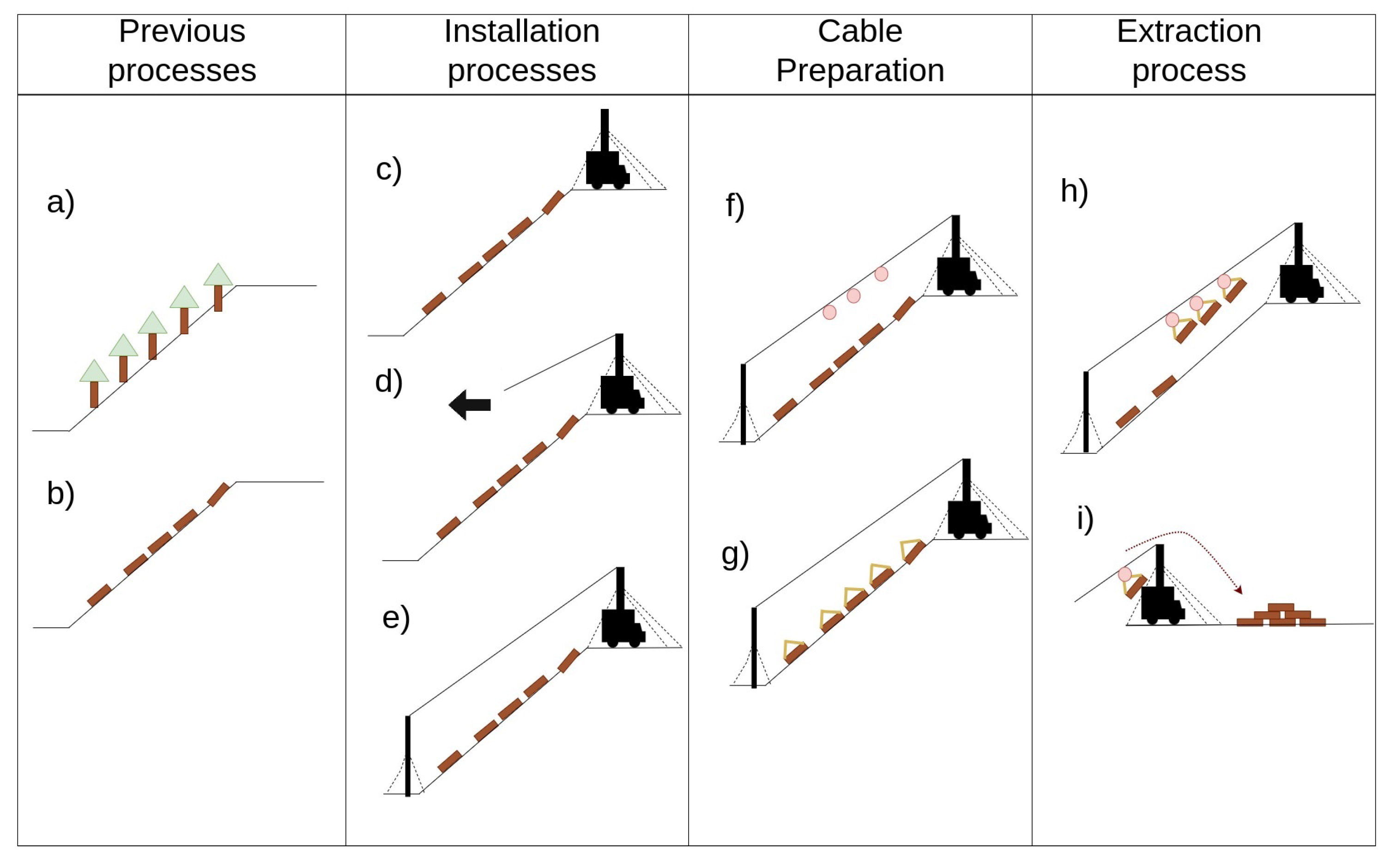
Skyline tower harvesting is a logging method that employs mechanized towers to access trees on steep or challenging terrain. Utilizing extraction cables attached to each tree, this technique is typically employed in areas with high slopes where traditional access to timber is not feasible. Equipped with a lifting platform and cable system, these towers enable operators to safely cut trees from above, resulting in a more efficient and less environmentally damaging approach than conventional logging methods. However, this method also presents drawbacks, such as the high cost of machinery, specialized training requirements, and increased workplace accident risks. Trees must be felled, prepared for extraction using specialized slope techniques, and arranged for rapid removal (see Figure 1a,b). The cables are installed via a tower or logging cable that necessitates intermediate and final supports to ensure its stability, load support, and process continuity as the load is raised to the unloading area at the top of the slope (see Figure 1c). Installation of the extraction cable should be conducted from the yarder tower to the anchor point, typically by specialized technicians (see Figure 1d,e).

Upon completing the cable installation, the extraction process, known as “Full Tree,” begins. A carriage is installed on the skyline (see Figure 1f), and trees are secured to the cable in a process called bracing, which attaches them to the cart running along the logging cable (see Figure 1g). The cart is then retracted, and trees are dragged over the slope to the landing site or logging yard. At this location, trees are unloaded, cut, sorted, and transported to industrial facilities (see Figure 1h,i). Notably, a single cable can extract multiple trees per cycle, often between two and eight trees, depending on factors such as the machinery power and resistance, slope, cable tension, tree size, and other terrain aspects. A tree recovery round is referred to as a logging cycle, and minimizing the number of cycles is essential for reducing labor costs.

The environmental impact of aerial timber extraction is significantly lower than that of land-based methods. Ground-based extraction often leads to soil erosion as timber is moved down slopes, negatively affecting the soil quality. Consequently, the employment of aerial extraction methods with reduced operating times is crucial for mitigating the environmental challenges of this type of harvest.

The economic dimension of the extraction process warrants a mention. Specifically, the cost associated with setting up skylines plays a pivotal role in the planning phase, as it directly impacts the process’ economic feasibility. Should the installation expenses surpass the returns from the harvest, cable extraction will become nonviable.

A crucial aspect of the timber extraction process is the installation and removal times for the entire operation. As mentioned earlier, using a skyline system for “clean” extraction requires the installation of one or more towers on a given property. The position of the tower’s “foothold” must also be strategically determined to maximize tree extraction. Additionally, each cable has a specific timber capacity per logging cycle, resulting in combinatorial challenges that are often intractable [3]. Consequently, an optimization problem must be defined to minimize installation times for the cable extraction problem, considering both geometric and capacity constraints.

Numerous studies have addressed cable tree extraction and optimization. In [3], the facility location theory is employed to assign lines to different properties. In [4], the extraction costs of timbers are minimized using Geographic Information Systems (GIS) data and a heuristic that minimizes harvest costs is introduced. The work described in [5] proposes a tabu search that tackles two forest harvesting problems: machinery location selection and access network design for extraction. The authors compare their approach with a mixed programming mathematical model using CPLEX, demonstrating that the tabu search achieves better results with less computational time. In [6], various mathematical models based on [3] are presented for steep terrain with different cable lengths, demonstrating their applicability in 18 plans. A metaheuristic for the European Cableway Location Problem is introduced in [7], where a heuristic and a greedy metaheuristic are tested with test instances and a real case. The authors argue that both approaches are equally effective and could potentially minimize costs in the planning process. In [2], a mixed-integer linear programming approach is presented to minimize road design costs for vehicles and cable design. The results are compared to [1], with computation times ranging between 4 min and 8 h. In [8], two new formulations for the cable tree removal problem are introduced based on a model presented in [6]. The approaches yield favorable results depending on the specific parameters used for the problem.

Several scientific studies focused on the monitoring of extraction cables have been published recently. A notable one is the article from [9], which details a monitoring system that uses the Geographical Navigation Satellite System (GNSS). With this system, the authors manage to identify 98% of the measured cycles, providing valuable data for the analysis of cables and their operations. In a different approach, the study presented in [10] concentrates on the physical state of the cables, comparing tensile forces to static calculations. To address the inherent limitation of static data, a simulation based on finite elements (FEN) was employed. The researchers suggest that the FEN simulation is useful for analyzing the tensile forces of the horizon. Going a step further in complexity, the article presented in [11] examines the forces affecting the extraction cables by adopting a nonlinear approach. This method provides a comprehensive solution, allowing adaptations based on specific configurations by adding equations to the existing system. Lastly, the article [12] proposes a predictive method for the cable trajectory using software called Seilaplan, which is specifically designed for cable extraction technologies in Central Europe. The accuracy of the predictions is based on the Zweifel approach and was validated with real data, demonstrating reliable results, as measured by RMSE values. In this way, the importance of the study of extraction cables for forestry harvesting is evident, and the study is very important for different aspects of the forestry field.

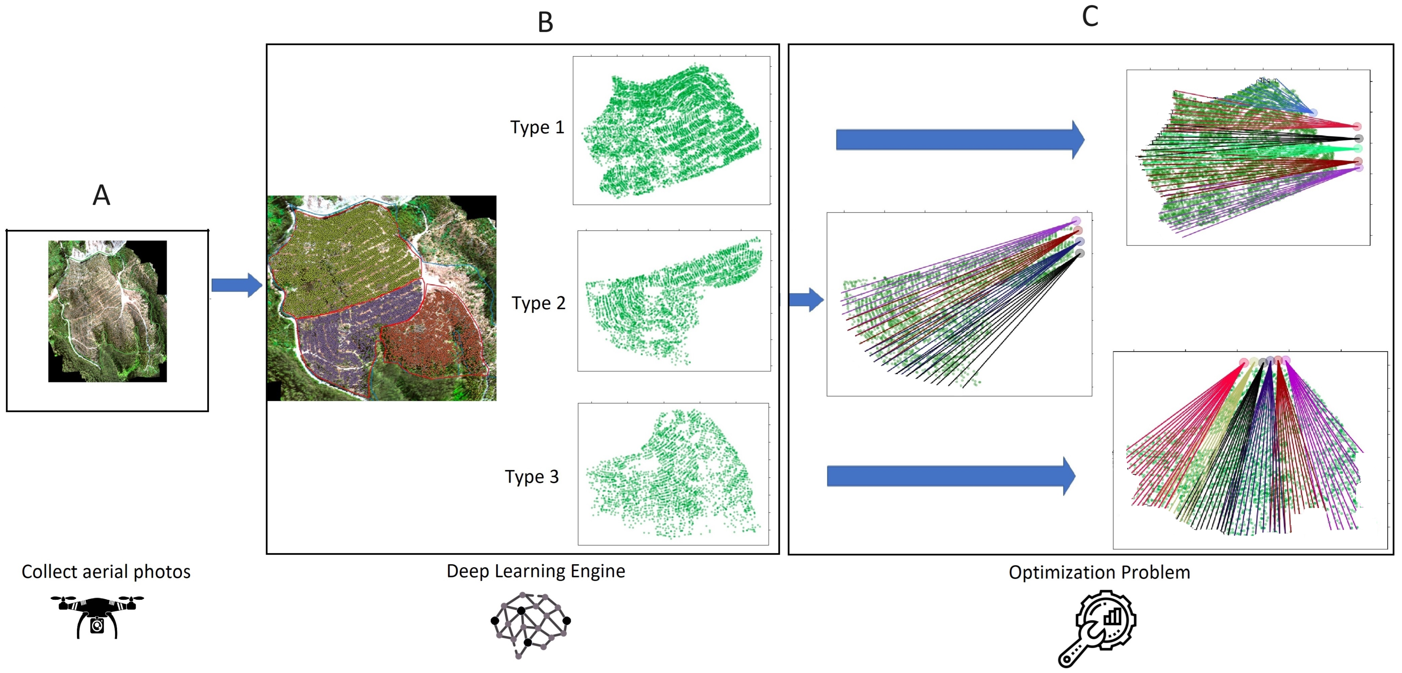
One of the primary factors that determines the efficiency and yield of forest harvesting with Skyline Towers is the placement of logging lines, which depends heavily on the forest conditions and tree positions on the slope. Accurate information about tree locations and sizes is crucial during the harvest planning phase. Typically, highly experienced operators make decisions based on their expertise, as this information is not readily available before a harvesting operation. Having precise tree locations would facilitate the definition of logging cable directions, the determination of intermediate and final support trees, the estimation of the number of logging cycles for each line, and the calculation of harvest yields, times, and costs more accurately. Moreover, it would help to minimize environmental costs by reducing soil compaction caused by logging lines. Improved harvest planning can be achieved with high-quality cartography and aerial images, which most harvesting companies possess. However, this requires a pre-processing phase for information. Deep Learning, a branch of Artificial Intelligence, can identify and segment objects within an image, making it possible to locate individual trees in a forest. The authors of this research are developing a Deep-Learning-based platform to identify and locate trees in Skyline Tower harvest sectors, which can then serve as the input for mathematical optimization processes to solve the problem of optimal logging cable allocation. This approach enhances the precision and efficiency of forest harvesting operations while minimizing environmental impacts.

Although the presented results are competitive, it is essential to introduce metaheuristics that minimize installation and operation times for large-scale planning with manageable durations. This article defines a binary mathematical programming model to optimize the installation and removal of timbers in cable logging operations. The model considers the tree allocation to cables, optimal cable selection based on the tower and stringer, cable intersections, and the extraction cable capacity. Furthermore, a hybrid approach is introduced to address the problem: a genetic algorithm assigns trees to lines and minimizes their number, followed by a mathematical model that utilizes the best individual to solve the logging cycle problem concerning the cable capacity. Lastly, comprehensive computational results are showcased, in which the manual planning approach (MPA) is compared with those generated using mathematical models. Additionally, a comparison is drawn with our two-phase algorithm. All discussed approaches are tested under real-world scenarios.

The rest of this article is organized as follows: in Section 2, we present the problem modeling related to the issue at hand. Section 3 introduces the integer mathematical programming formulation for the problem. Section 4 describes the two-phase approach, which employs a genetic algorithm and a mathematical model based on Section 3 to generate logging cycles. Section 5 provides details of the computational experiments, while Section 6 concludes our article with a summary of the findings.

2. Related Work—Modeling of the Cable Extraction Problem

The tree extraction process begins in a predetermined sector where each tree’s location, weight, and extraction time—the duration it takes to move the tree from the ground to a cable—have been meticulously cataloged. These trees are then transported to a specific area for stacking in anticipation of their subsequent removal by trucks. The primary aim of this model is to streamline the sequence of tree extraction from the ground to the landing area while optimizing the selection of extraction cables. This strategy is designed to decrease the overall operational times, including those required for installing a tower, setting up cables, tree extraction, and the complete logging cycle.

2.1. Yarder Installation Time

The installation time for a yarder varies based on its location and the specific model of the tower being used. We maintain the installation time in the tower model for our model, allowing only the installation site to vary. This site is typically located within the landing area, where the trees are gathered for stacking. The extraction operation’s specific location fundamentally determines the tower’s quantity and positioning.

2.2. Cable Installation Time and Tree Removal

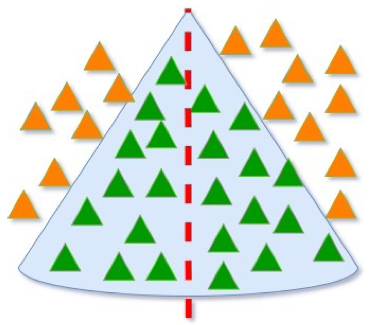
An array of cables stemming from various yarders is crucial for tree extraction. It is essential to judiciously select the appropriate cables to ensure an efficient extraction process. Every cable corresponds to a potential extraction area that takes the shape of a cone, as illustrated in Figure 2. This cone-shaped area signifies the space within which the cable can operate effectively, thereby delineating its range of extraction. The design of this cone is crucial, as it governs the cable’s extraction capacity and operational efficiency.

Given the unique extraction area associated with each cable, every tree within the property under study must be extracted using a single cable. As such, each tree must be systematically aligned with a specific extraction cable dictated by the spatial limitations of the defined cone-shaped logging. This constraint mandates a strategic mapping of trees to cables, ensuring that each tree falls within the operational boundaries of its assigned cable. This careful coordination maximizes the extraction efficiency and minimizes the potential damage to the surrounding forested area during the extraction process.

2.3. Logging Cycles

Every extraction line in a logging operation features an unique characteristic called logging cycles. These cycles are quantitatively defined by the number of trees a single cable can haul during a single procedure or turn. The cable’s reach and strength, the size of the trees, and the terrain all factor into this calculation, which is pivotal for efficiency and productivity. Each logging cycle is further associated with a set of variables that require careful optimization. Firstly, there is the cycle time—the duration it takes to complete one extraction cycle. The aim is to minimize this time without compromising safety or efficacy, as it directly impacts the overall productivity of the logging operation. Faster cycle times mean that more trees can be extracted per unit of time, thereby enhancing the throughput and efficiency of the logging process. Secondly, there is the concept of cycle capacity. This term relates to the maximum effort or forces that the extraction line can exert in a single cycle, which in turn depend on the weight of the tree to be extracted and the distance between the tree and the logging line. This capacity must be sufficient to haul the tree from its original position to the extraction point. Factors such as the size and weight of the tree, the cable type and condition, the land gradient, and the distance to be covered all play roles in determining the cycle capacity.

In essence, these two parameters—cycle time and cycle capacity—are critical for logging operations. They must be carefully balanced and optimized, as they directly influence the extraction process’ efficiency, safety, and productivity. By understanding and improving these aspects, logging operations can significantly increase their performance and sustainability.

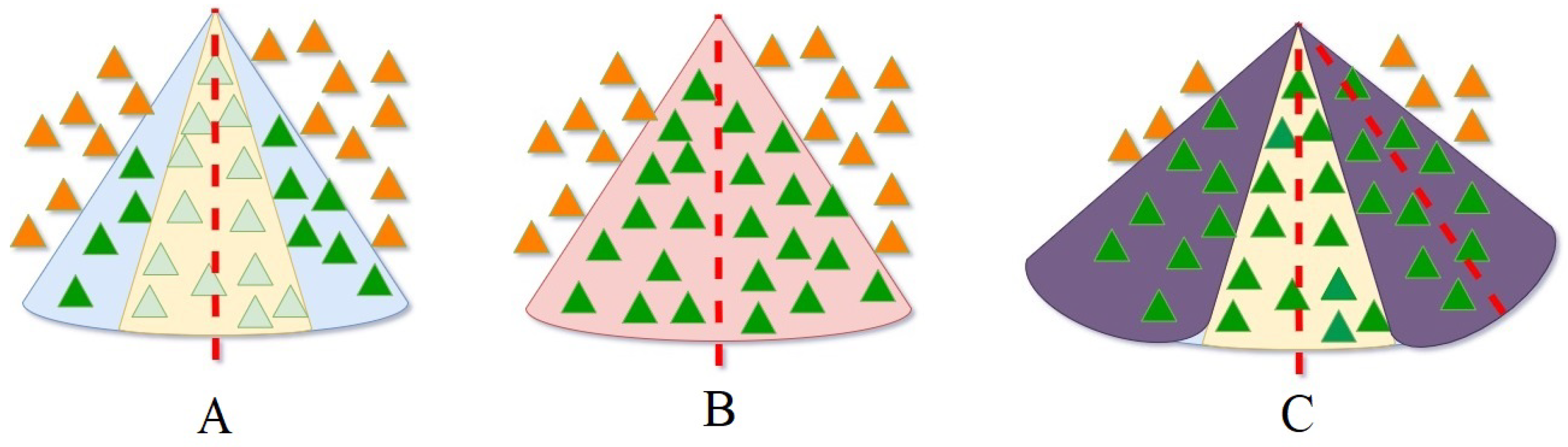
The capacity of a logging cycle is a critical threshold that an extraction line must respect. Figure 3 illustrates the various states of an extraction line. In Figure 3A, the blue area represents potential extraction, but the line capacity restricts extraction to trees within the yellow cone. Figure 3B depicts a saturated line with a red cone, where assigning all trees from the potential area is impossible. Figure 3C presents a scenario with three extraction cables; the central wire is unsaturated due to the allocation of trees to the surrounding cables.

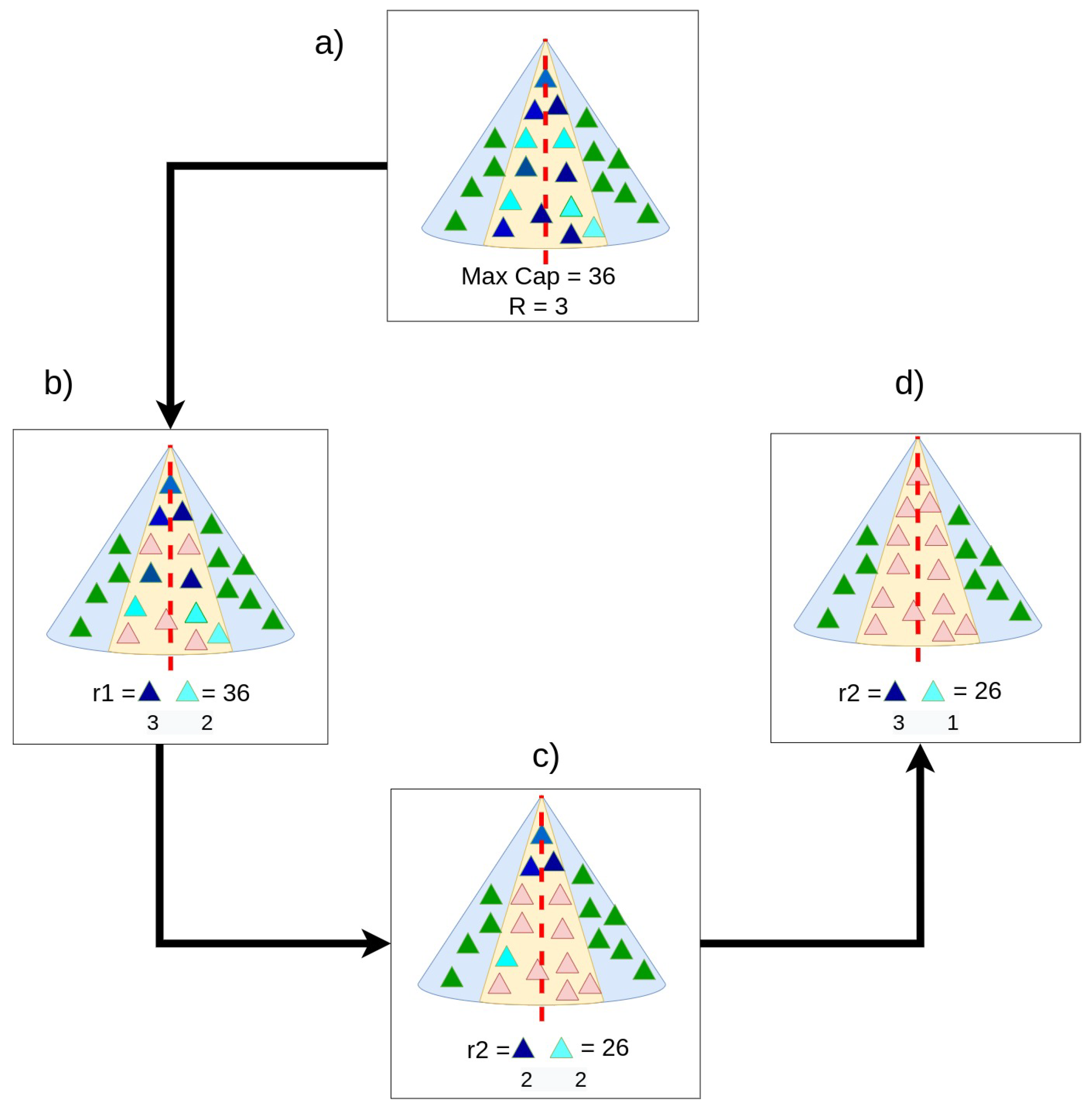
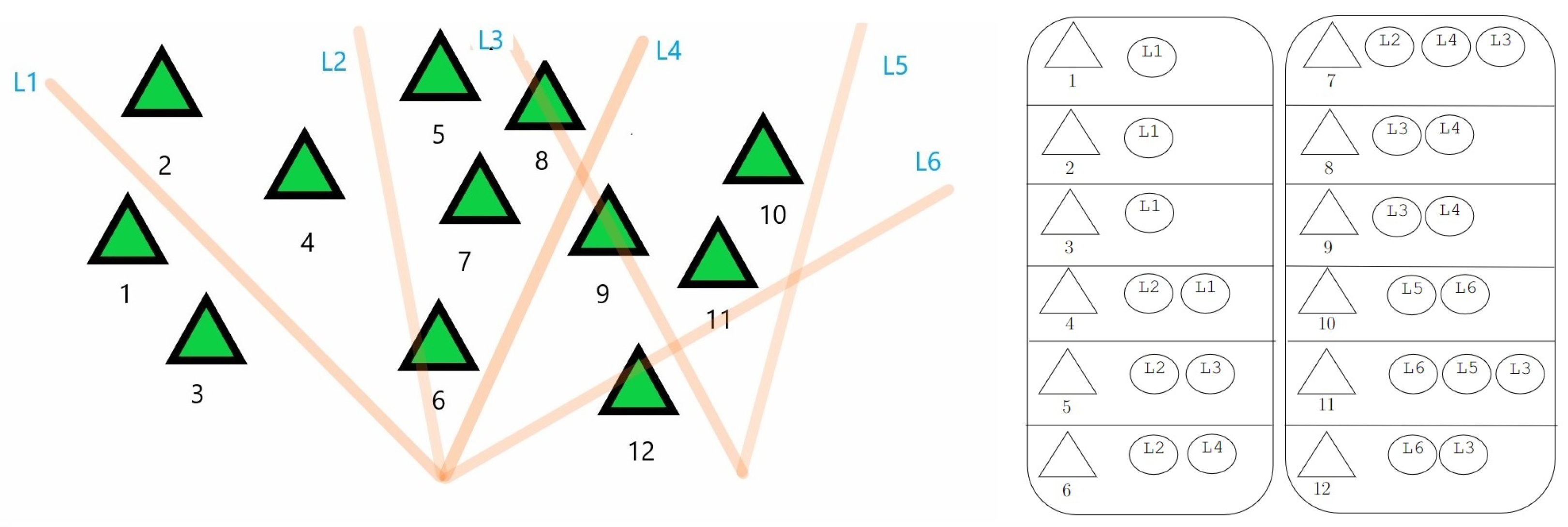
Each extraction cable possesses a capacity specific to its respective logging cycle. Figure 4a shows the timber cycle concept by defining a simple area notation: green triangles represent trees that are accessible to the cable but not assigned to it. In contrast, light blue triangles signify trees that are assigned to the cable and hence to a logging cycle. The extraction cable can execute three logging cycles ($R=3$) with a maximum capacity of 36 units per cycle. Trees depicted as light blue triangles consume three units of cable capacity, while the blue triangles utilize ten units. In the first logging cycle, $r1$, shown in Figure 4b, three blue triangles (3 × 10 = 30 capacity units) and two light blue triangles (2 × 3 = 6 capacity units) are extracted. This results in the feasible cycle capacity of 36 units being fully utilized. The extracted triangles are marked in red. The second logging cycle, $r2$, represented in Figure 4c, extracts two blue triangles (2 × 10 = 20 capacity units) and two light blue triangles (2 × 3 = 6 capacity units), yielding a feasible capacity utilization of 26 units. Finally, the third and last logging cycle, $r3$, shown in Figure 4d, extracts three blue triangles (3 × 10 = 30 capacity units) and one light blue triangle (1 × 3 = 3 capacity units), thereby utilizing a feasible capacity of 33 units.

2.4. Description of the Problem

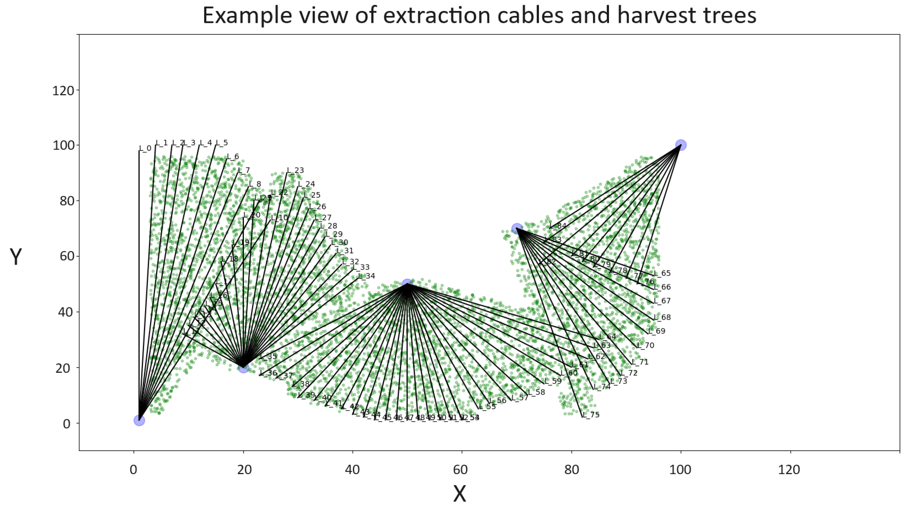
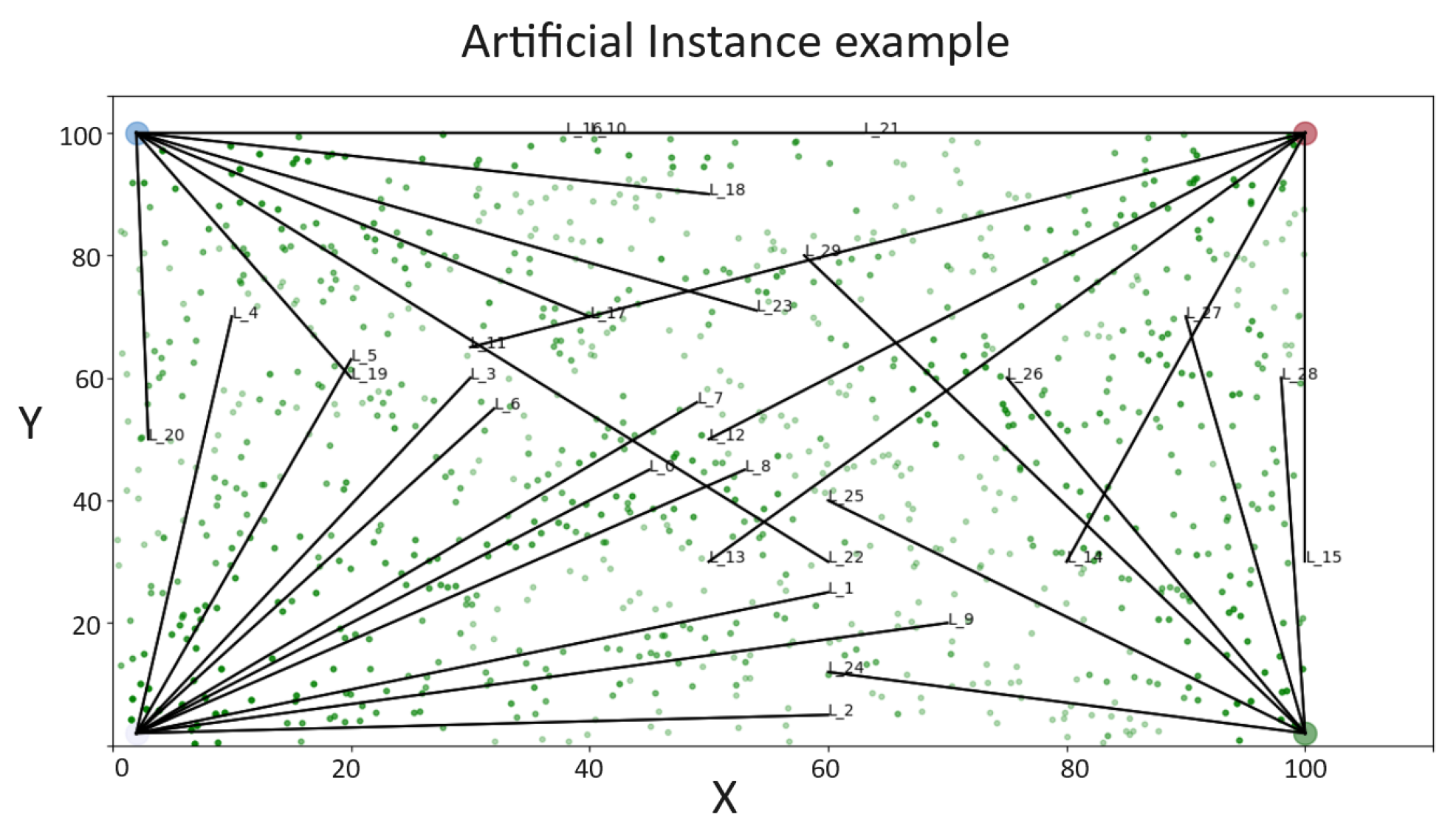
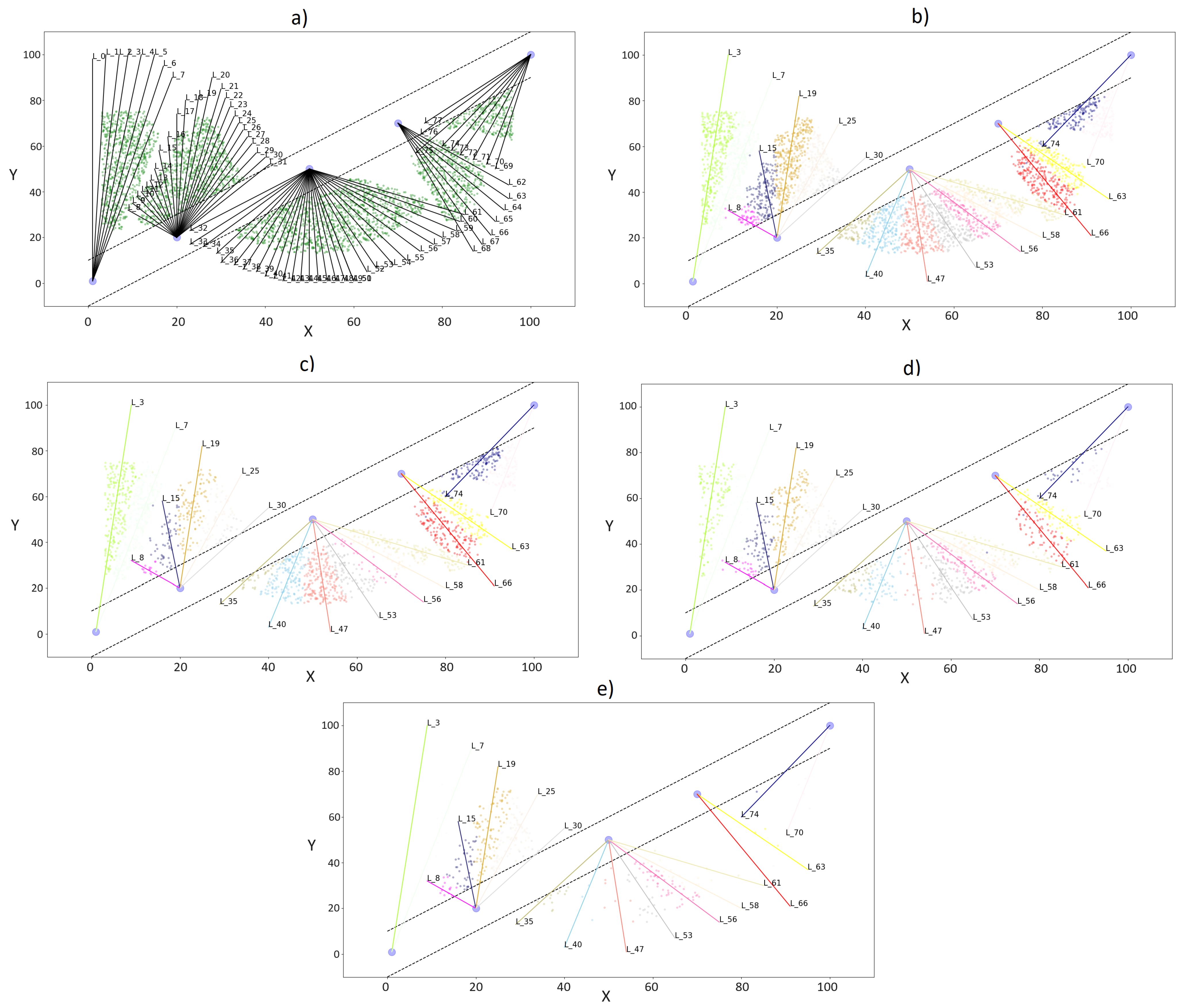
Every tree in a designated sector must be fully extracted, as illustrated by Figure 5, which presents a typical example for this process. The example scenario presented was artificially generated to better explain the completeness of the problem. The depicted stage features five towers, each equipped with an extraction cable. As Figure 2 demonstrates, every cable possesses a corresponding extraction logging cone. These cones can overlap with adjacent logging cones, creating areas of intersection. However, a tree falling within this intersection must be exclusively associated with a single line to avoid conflicts and ensure efficient extraction. The example also reveals intersections between different cables, a situation that should be avoided when selecting cables for this task. Overlapping lines could lead to confusion in the assignment of trees and reduce the overall efficiency of the logging process.

In the following section, a mathematical model is introduced. This model effectively addresses the challenge of assigning trees to individual lines and selecting the optimal lines to ensure the most efficient extraction process is produced.

3. Problem Description and Mathematical Formulation

A mathematical model can be defined to solve the tree assignment problem. For this reason, the indices, sets, variables, and parameters are defined. First, the indices are determined: for the tree selection $t\in T$, for the yarder selection $y\in Y$, for the extraction cable selection $l\in L$, and indices for a single revolution of a single cable $r\in R$. Second, previously defined sets of cables are determined depending on the geometry: $I\left(l\right)\in L$ corresponding to a set of cables that intersects cable l and $L\left(y\right)\in L$ corresponding to a set of cables that starts from the yarder Y. The parameters are shown in

Table 1. Parameters of the mathematical model.

Parameter	Description
$D_y$	Time needed to install the yarder $y\in Y$.
$P_{yl}$	Time needed to install the cable $l\in L\left(y\right)$.
$H_{lt}$	Time needed to extract $t\in T$ for the cable $l\in L$.
$Z_{lr}$	Time needed to generate a single revolution r by the cable l.
$W_{lt}$	Effort performed by the cable l to extract the tree t.
$C_{rl}$	Maximum number of trees that a single cable l can extract in a revolution r.

. In this way, the cables allow all of the trees of the problem with the following decision variables to be extracted:

• $w_y=\left\{\begin{array}{c}1iftheyarderyisused\\ 0otherwise\end{array}\right.$
• $c_l=\left\{\begin{array}{c}1ifcablelisused\\ 0otherwise\end{array}\right.$
• $x_{ltr}=\left\{\begin{array}{c}1ifthetreetisextractedwiththecableslintherevolutionr\\ 0otherwise\end{array}\right.$
• $z_{lr}=\left\{\begin{array}{c}1ifthelinelusestheloggingcycler.\\ 0otherwise\end{array}\right.$

The mathematical model minimizes the extraction and installation time of the problem subject to different constraints. The objective function in Equation (1) has four main components: minimizing the installation time of the selected yarder y, minimizing the installation time of the cable l that starts from the yarder y, minimizing the extraction of each tree t by cable l in revolution r, and minimizing the time that the logging cycle r belongs to the cable l. Constraint (2) ensures that every tree is associated with a single cable during a single revolution. Constraint (3) ensures that there is no infeasible selection of extraction cables for the problem considering intersections. To achieve this, it is essential to ensure that each cable $k\in I\left(l\right)$ does not intersect with the cable $l\in L$. Constraint (4) makes sure that the yarder y is selected if a cable $l\in L\left(y\right)$ is also selected. Constraint (5) makes sure that the cable l is selected if a tree t associated with the variable $x_{ltr}$ is selected. Finally, the model variables are defined in the Constraint (7).

$$min\sum _{y\in Y}{D}_y{w}_y+\sum _{y\in Y}\sum _{l\in L_y}{P}_{yl}{c}_l+\sum _{l\in L}\sum _{t\in T}\sum _{r\in R}{H}_{lt}{x}_{ltr}+\sum _{l\in L}\sum _{r\in R}{Z}_{lr}{z}_{lr}$$

(1)

s.t

$$\sum _{r\in R}\sum _{l\in L}{x}_{ltr}=1\forall t\in T$$

(2)

$$c_l-M\sum _{k\in I\left(l\right)}(1-c_k)\le 0\forall l\in L,$$

(3)

$$\sum _{l\in L\left(y\right)}{c}_l\le M{w}_y\forall y\in Y$$

(4)

$$\sum _{r\in R}\sum _{t\in T}{x}_{ltr}\le M{c}_l\forall l\in L,$$

(5)

$$\sum _{t\in T}{W}_{lt}{x}_{ltr}\le C_{rl}{z}_{lr}\forall l\in L,\forall r\in R$$

(6)

$$w_y\in \{0,1\};c_{lp}\in \{0,1\};x_{ltr}\in \{0,1\};z_{lr}\in \{0,1\}$$

(7)

The following section defines a two-phase algorithm to solve the proposed problem: a genetic algorithm that solves the allocation of the trees for a single line and a mathematical model that performs the logging cycles for the best solution from the genetic algorithm.

4. Two-Phase Approach to Solve Cable Logging

The problem formulated above can be described in two fundamental processes (phases): assigning trees to lines and generating logging cycles. Tree assignment can be performed in a (meta)heuristic way with a genetic algorithm (GA). Subsequently, the solution developed by GA can be used by a mathematical model that will generate the logging cycles for each logging line (phase 2).

Genetic algorithms were proposed by Holland [13] and are the most representative technique of evolutionary computation. The method follows a process based on the evolution of the species where the best individual survives in subsequent generations [14]. Generally, an individual of the genetic algorithm is represented in an array (chromosomes) with numbers in each of their positions (known as genes). The details of this metaheuristic can be seen in Algorithm 1: first, individuals are randomly generated (line 1) with a defined population size $n_{pop}$. Subsequently, the generated population is subjected to a number of generations $n_{gen}$ (line 4) with different fundamental processes: the evaluation of each individual through a fitness function (line 5), the selection of the best individuals in a random way (line 6), a crossover of individuals with the probability $c_x$ (line 7), and the mutation of individuals with a probability of occurrence $m_x$ (line 8). Finally, a mathematical model is applied to the allocation generated by the GA to generate the log cycles. The details of each process are described in the following subsections.

Algorithm 1 GA for Cable Logging.

Require: Parameters: $n_{gen},n_{pop},c_x,m_x$

Ensure: Solution: $S^{*}$ 1: $InitialPopulation=RandomProcedure\left(n_{pop}\right)$         ▹ Phase 1 2: $P^{*}=InitialPopulation$ 3: $gen=0$ 4: while $gen<n_{gen}$do 5:     $P^f=FitnessProcedure\left(P^{*}\right)$ 6:     $P^s=Selection\left(P^f\right)$ 7:     $P^c=Crossover(P^s,c_x)$ 8:     $P^{*}=Mutation(P^c,m_x)$ 9:     $gen=gen+1$ 10: end while 11: $bestIndividual=BestIndividual\left(P^{*}\right)$ 12: $S^{*}=GenerationOfLoggingCycles\left(bestIndividual\right)$      ▹ Phase 2 13: return $S^{*}$

4.1. Representation of an Individual

First, a data structure for the extraction problem must be defined. Figure 6 represents a small example of the representation of a problem: on the left side of the image, the problem is displayed geometrically, i.e., the trees that must be extracted are presented in green triangles numbered from 1 to 12 and the potentials of the cable (orange) that must be selected are numbered from 1 to 6. On the right of the image, the data structure is presented: each of the trees has potential extraction lines to which it can be assigned. The logging lines are sorted by distance, so the structure always keeps the nearest (cheapest) lines in first place. For example, tree 11 can be extracted by cable 6 (nearest), cable 5, and cable 3 (farthest, but feasible).

The representation of an individual in the GA involves mapping a tree to a valid cable within the data structure. Each gene represents the assignment of a tree to a (single) cable; thus, the length of the chromosome is proportional to the number of trees on the farm. Figure 7 shows an example of a chromosome and the selection of lines for each tree. For this example, the first three alleles (trees) contain position 0 of their draw lines in the ordered structure, so they are assigned to their closest lines, alleles 4 and 5 are assigned to the second nearest lines, and so on.

Initially, for each gene, a uniformly distributed random number is generated with the range $[0,M]$ with M defined as the maximum number of trees between the logging lines of the plot (for this example, cones 7 and 11 are the largest with M = 3). Thus, the GA must define a feasibility process (i.e., converting an individual from infeasible to feasible). For it, the modulo function is used with the size of the lines of each tree. Figure 8 shows a structure that contains the number of lines for each tree according to the problem’s structure. The new valid chromosome is obtained by applying the modulo operator to the original chromosome with the correct size for each gene. Note that the modulo operation effect replaces only invalid genes; therefore, genes 3, 5, and 9 were changed.

4.2. Fitness Function

The fitness function must evaluate an individual’s qualification within the evolutionary process. For the cable extraction problem, it is necessary to quantitatively evaluate whether the cable selection is good. The function must carry out three fundamental processes: a ranking process, where lines that intersect each other must be eliminated; a cable minimization process, where a heuristic seeks to minimize the number of selected lines; and reassignment, where trees that were assigned to lines that were removed in previous processes must be reassigned to new final lines. Figure 9 shows the summary of the process.

4.2.1. Ranking Process

The first process within the fitness function is cable intersection removal. Let $G_l$ be a set of trees that are extracted by the cable l according to the chromosome to be evaluated, and let $V_l$ be a set of cables that intersect with the l line. The formula used for the ranking to evaluate each cable is described in Equation (8).

$$f\left(l\right)=\omega (\frac{G_l-MinG}{MaxG-MinG})+\theta (1-\frac{V_l-MinV}{MaxV-MinV})$$

(8)

Normalized values are considered in the ranking process. For this, the following values are calculated from the chromosome: $MinG$ corresponds to the cable that contains the least number of assigned trees; $MaxG$ corresponds to the cable that includes the largest number of assigned trees; $MinV$ corresponds to the least number of intersection cables; and $MaxV$ corresponds to the largest number of intersection lines. To consider both features (tree assignment and cable intersection), two factors are defined, such that $\omega +\theta =1$.

The lines are removed until the solution generated from the chromosome has no intersection. First, the lines are sorted according to the value of the Equation (8) in descending way. Subsequently, lines are removed until the solution does not present intercepted lines. Figure 9 shows that the original individual contains three intersecting lines (yellow, green, and red lines). According to Equation (8), the cable with the lowest score is presented in yellow, the next in green, and the next in red. Finally, the yellow and green lines are removed (in the order described above). Note that the red line is not removed since the solution does not have cable intersections. Trees that had been assigned to deleted lines are shown in light blue.

4.2.2. Cable Number Minimization Process

The solution presented for this process uses a large number of lines. In this way, the lines considered from the previous process are subjected to elimination with a greedy heuristic based on the Set Covering problem [15]. The heuristics can be seen in Algorithm 2.

Algorithm 2 Greedy Heuristic Delete.

Require: $Trees$ T, $Lines$ $Cost$ $of$ $lines$ C ($\forall l\in$ Chromosome), $Subset$ S ($\forall l\in$ Chromosome)

Ensure: F  $FinalLines$ 1: $cost=0$ 2: $covered=\varnothing$ 3: $NotCovered=T$ 4: $F=\varnothing$ 5: while $covered$  $!=$ T do 6:     $(tset,l)=$ set of tree with highest: $\left(\frac{|S_l\setminus covered|}{c_l}\right)\forall l\in$ Chromosome $and$ $l\notin F$ 7:     $cost=cost+C_l$ 8:     $covered=covered\cup tset$ 9:     $NotCovered=T\setminus covered$ 10:     $F=F\cup \left\{ļ\right\}$ 11: end while 12: return F

The final lines are selected using the cost of each of them. Algorithm 2 iteratively considers the best lines according to the number of trees that l extracts (trees that other lines in previous iterations have not evaluated) and the cost of the cable l (line 7). The highest value is listed in F, and the algorithm continues until all problem trees have been considered. Note that the number of trees in the operation $|S_l\setminus covered|$ considers the total number of trees that a cable can extract. Figure 9 shows the output of the minimization process. For this case, the orange and the plumb cable are removed. Again, trees that had been assigned to deleted lines are shown in light blue.

4.2.3. Tree Assignment

Finally, the trees deallocated in previous processes are assigned to non-deleted lines (set F from the greedy algorithm). Trees are assigned to the nearest valid cable from F. Figure 9 shows the cyan trees of previous processes assigned to the lines belonging to F (purple, blue, and red).

4.2.4. Final Formula

The fitness function must assign a quantitative value to the solution generated from the chromosome. Once the final individual is obtained from the previous processes, Equation (9) is used, which can be divided into three parts: the installation time of the yarders, the installation time of the lines, and the extraction time of each tree according to the associated line. This value will be used for the genetic algorithm selection process.

$$f\left(Chrom\right)=\sum _{y\in Y\left(Chrom\right)}{D}_y{w}_y+\sum _{y\in Y}\sum _{l\in Chrom}{P}_{yl}{c}_l+\sum _{l\in Chrom}\sum _{t\in T}{H}_{lt}{x}_{lt}$$

(9)

4.3. Selection

Roulette selection was used. This method assigns a proportional adjustment value to a roulette using its fitness value. In this way, the best individuals receive a more significant proportion in the roulette, having a better chance of being selected. Individuals are selected without replacement until the overall GA process is complete [16].

4.4. Crossover

Crossover selects two individuals (called parents) with a given probability $cx$ from the subpopulation generated by the selection. A random number $\gamma$ between zero and one (without considering one) is chosen to select the number of genes to cross $n=\left|T\right|*\gamma$. The integer part of the result obtained is considered for n. Subsequently, two genes are randomly selected n times and swapped. Finally, the two new individuals are returned. Figure 10 considers an example of the operator.

4.5. Mutation

Two mutation operators are defined for this evolutionary process. The first operator randomly changes half of the genes to valid cones, while the second operator applies a local search on half of the genes, selecting the best cable from the chosen tree. The first and second operators are applied with probabilities $\alpha$ and $\beta$, respectively. A flowchart in Figure 11 is shown, using the ordered structure proposed in Section 4.1.

4.6. Generation of Logging Cycles

A mathematical model is developed to generate a feasible solution from the GA solution. The model aims to minimize the time cost of the logging cycles, as shown by the objective function (10). The original model includes restrictions (11)–(14) defined below. However, the model only considers the lines selected from the best individual (variable $Chrom$ in the model).

$$min\sum _{r\in R}{Z}_{lr}{z}_{lr}$$

(10)

s.t

$$\sum _{r\in R}\sum _{l\in Chrom}{x}_{ltr}=1\forall t\in T$$

(11)

$$\sum _{r\in R}\sum _{t\in T}{x}_{ltr}\le M{c}_l\forall l\in Chrom,$$

(12)

$$\sum _{t\in T}{W}_{lt}{x}_{ltr}\le C_{rl}{z}_{lr}\forall l\in Chrom,\forall r\in R$$

(13)

$$c_l\in \{0,1\};x_{ltr}\in \{0,1\};z_{lr}\in \{0,1\}$$

(14)

5. Experimental Evaluation

5.1. Benchmark Instances

To measure the performance of the mathematical model and the genetic algorithm, we must define a set of instances. In this way, we generate two groups of instances: instances generated randomly and instances generated from a real scenario.

5.1.1. Random Instances

We used artificial areas with characteristics similar to a real scenario for the cable extraction problem. For this, nine instances were generated by positioning the trees with a uniform distribution. All instances were grouped into three groups according to the number of trees $\{1800,3000,5000\}$. In this way, three instance types were generated according to their groups (Figure 12).

5.1.2. Real World Instances

Our approaches were also tested on a set of instances derived from real-world scenarios. For an accurate study, we utilized data captured from UAVs, specifically aerial photographs (refer to Figure 13A). After obtaining these photos, Deep Learning models were employed to identify tree canopies, which enabled us to pinpoint their locations on a Cartesian map (as illustrated by Figure 13B). The images were processed using two fully convolutional neural network architectures: YOLO [17] and Mask [18]. The details of the classification can be found in [19]. Concluding this process, we positioned the candidate lines using the yarders and anchor points, which served as the input optimization problem for our delineated approaches (refer to Figure 13C).

5.1.3. Instance Parameters

Instance parameters are derived from physical attributes and the average speed at which a cable can haul timber within its logging cone. Accordingly, for each set of instances—whether artificial or rooted in real-world scenarios—distinct parameters are outlined in Table 1, encapsulating the essence of the problem. Installation times (for cables and yarders) were sourced in consultation with forestry harvesting specialists. Meanwhile, extraction times were determined by the perpendicular distance between the timber and the cable extraction point and the extraction speed from the timber collection point to the landing site. The extraction speed decreases as the distance from the logging tower to the timber increases.

5.2. Experimental Protocol

The mathematical model was tested on Gurobi 9.5.2 and CPLEX 20.0 with Python 3.7 with Threads = 1. We generated the GA implementation in Python 3.7. The experiments were carried out in a cluster with Intel Xeon Cascade Lake CPU 3.10 GHz with eight cores and 32 GB RAM using Ubuntu 19.04.

5.3. Parameter Calibration for the GA

We used the iterated racing for automatic algorithm configurations (IRACE) method (proposed in [20]). The framework applies an elitist procedure, which iteratively samples parameter combinations according to a certain probability, selecting the best ones and discarding those that lead to low-quality results. In each iteration, samples are updated, and the parameter values with the best performances increase their probabilities of being selected. We used the three smallest size instances for the calibration process. The search space parameters of the GA are as follows: number of generations = $\{10,15,20,50\}$, number of population = $\{50,100,150,200\}$, and probability of crossing = $cx=\{0.8,0.85,0.9,0.95\}$. The mutation was defined as $mx=1-cx$ with $\alpha =0.5$ and $\beta =0.5$. Parameter $\theta =\{0.3,0.5,0.8\}$ with $\omega =1-\theta$ was defined for the ranking function. Finally, $\gamma =\{0.5,0.6,0.7\}$ was defined for the internal crossing process.

The details of the instance groups are presented in

Table 2. Parameters obtained from IRACE.

ID	N° Gen	N° Pop	$\mathbf{cx}$	$\mathit{\theta }$	$\mathit{\gamma }$
Set1	10	100	0.8	0.5	0.6
Set2	15	100	0.7	0.5	0.6
Set3	10	150	0.9	0.5	0.6

.

As a concluding step in our study, we implemented the GA under the Set 1 configuration. The choice to highlight this particular configuration arose from comparing various algorithm configurations. The Set 1 configuration, as it turned out, consistently outperformed others in the tests. It delivered superior results in most instances and demonstrated improved stability and effectiveness.

5.4. Computational Results

The results of the computational experiments are divided into two sections: “Results for Random Instances”, which details the time required to achieve effective scheduling with the instances generated for the research, and “Results for Real Cases”, where the outcomes obtained through the use of Deep-Learning-processed images are presented.

5.4.1. Results for Random Instances

Table 3. Results from Random Instances.

Type	ID	MPA		Gurobi 9.5				CPLEX 20				GA + Model
		Value	Time (s)	Value	Bound	% Gap	Time (s)	Value	Bound	% Gap	Time (s)	Min	Average	Stdev	% Gap GRB	% Gap CLPX	Avg, Time (s)
1	1	22,158.15	1.70	17,966.88	16,848.81	6.22	500.52	18,160.08	16,870.29	7.10	500.65	18,052.54	18,252.15	369.86	0.48	−0.59	105.97
1	2	19,592.29	4.36	17,552.17	16,188.59	7.77	500.03	17,803.75	16,242.15	8.77	500.65	17,493.17	17,776.86	364.05	−0.34	−1.74	83.91
1	3	238,650.30	1.49	16,441.73	16,178.73	1.60	500.04	17,195.66	16,099.76	6.37	500.62	17,111.66	17,912.59	432.03	4.07	−0.49	97.88
1	4	20,579.87	1.51	18,630.30	17,190.83	7.73	500.04	20,584.23	17,217.00	16.36	500.75	18,393.62	19,180.16	486.58	−1.27	−10.64	250.30
1	5	24,676.71	1.56	18,090.01	16,976.40	6.16	500.05	18,088.39	16,963.45	6.22	500.82	18,908.15	19,298.59	262.76	4.52	4.53	212.23
	Average	65,131.46	2.12	17,736.22	16,676.67	5.89	500.14	18,366.42	16,678.53	8.96	500.70	17,991.83	18,484.07	383.06	1.49	−1.79	150.06
2	1	28,509.12	6.02	21,124.22	16,470.86	22.03	500.06	20,812.62	16,769.83	19.42	500.49	19,758.39	19,942.10	269.37	−6.47	−5.07	326.84
2	2	25,443.90	7.15	20,884.90	17,354.36	16.90	500.06	21,739.64	17,370.32	20.10	500.61	19,045.32	19,384.69	334.45	−8.81	−12.39	347.67
2	3	22,040.33	7.66	19,465.47	16,889.59	13.23	500.06	19,476.64	16,864.49	13.41	500.84	19,027.99	19,635.88	408.00	−2.25	−2.30	322.53
2	4	21,870.38	6.56	19,718.86	16,360.85	17.03	500.06	20,211.75	16,436.03	18.68	500.62	18,157.08	19,000.20	586.92	−7.92	−10.17	337.71
2	5	23,500.14	8.40	19,746.28	16,481.55	16.53	500.06	19,859.69	16,733.74	15.74	501.05	19,546.61	19,717.03	109.22	−1.01	−1.58	334.04
	Average	24,272.77	7.16	20,187.94	16,711.44	17.15	500.06	20,420.07	16,834.88	17.47	500.72	19,107.08	19,535.98	341.59	−5.29	−6.30	333.76
3	1	26,323.81	5.69	19,792.43	16,506.18	16.60	500.18	19,586.41	17,039.96	13.00	501.68	19,675.85	19,904.70	114.49	−0.59	0.46	360.80
3	2	23,528.93	6.03	19,665.36	17,180.61	12.64	500.08	22,326.64	17,245.17	22.76	500.80	19,787.48	20,296.25	274.98	0.62	−11.37	355.28
3	3	25,039.41	4.35	20,635.61	16,217.32	21.41	500.08	22,995.42	16,745.47	27.18	500.76	20,362.93	20,998.38	223.29	−1.32	−11.45	350.29
3	4	26,381.36	10.03	19,366.54	16,310.69	15.78	500.07	23,842.00	16,824.51	29.43	500.51	19,298.99	19,510.32	340.02	−0.35	−19.05	367.10
3	5	26,772.86	5.03	22,568.41	16,588.80	26.50	500.08	19,897.66	17,031.13	14.41	500.91	20,024.01	20,486.10	256.26	−11.27	0.63	354.34
	Average	25,609.27	6.23	20,405.67	16,560.72	18.58	500.10	21,729.63	16,977.25	21.36	500.93	19,829.85	20,239.15	241.81	−2.58	−8.16	357.56

presents the experimental results derived from the random instances. Comparisons were made between different schedules using three different approaches:

• Manual Planning Approach (MPA): This method assigns the first line from left to right and performs the extraction. The extraction time simulates a plan’s outcomes without a smart optimization approach. In other words, the time obtained in this schedule is similar to the time that would be achieved with a manual plan.
• Gurobi 9.5 and CPLEX 20.0: The results from these approaches are obtained from the solvers most commonly used in the academic literature. The mathematical model used is the one proposed in Section 3.
• GA + Model: This result is achieved through a two-phase approach.

We used metrics commonly used in operations research to compare the solvers utilized in the experiments. Initially, each solver determines a feasible solution value (VS), a lower bound (LB) for the searching process, and the computational time required. Subsequently, the %gap is calculated to assess the quality of the solution using the formula: %gap = ((VS − LB)/VS) × 100. When the upper bound matches the feasible solution value, the %gap becomes zero, signaling the end of the search. At this juncture, the solvers have identified the solutions to the problems under study.

Each column in the table represents the final outcome of the extraction and installation process according to the objective function, expressed in minutes (value); the corresponding upper bound (bound), if applicable; the internal gap percentage between the value and the upper bound (%gap); the computation time; the standard deviation obtained with the two-phase approach; the gap percentage relative to the solvers (%gap GRB, %gap CLPX); and, finally, the average time taken for the different executions performed with the two-phase approach.

The planning performed using a MPA process tends to be longer than with any other approach. As can be seen in Table 3, regardless of the type of instance, the times are consistently longer when the MPA process is used. In particular, for the first group, this approach requires an average of 65,130 min. Consequently, the idea of obtaining schedules through a mathematical model emerges as a viable and efficient alternative.

The computation times for the different solvers and the two-phase approach fluctuate as the number of trees increases. Table 3 displays the execution times of each method used in this study. It is important to note that traditional solvers fail to find optimal solutions in most proposed cases with a time limit of TL = 500 s. Indeed, only for case type 1 with ID = 3 is the gap percentage between the feasible solution and the upper bound small: approximately 1% in Gurobi 9.5. In the other proposed instances, both solvers fail to converge toward an efficient solution compared to the two-phase algorithm.

On the other hand, the two-phase algorithm finds better solutions in less time compared to traditional solvers. On average, the two-phase approach takes 150.06 s for type 1 cases, while for type 2 and 3 cases, the average times are similar, 333.76 s and 357.56 s, respectively.

The two-phase approach outperforms the traditional solvers. Table 3 shows two gap columns concerning CPLEX (%gap CLPX) and Gurobi (%gap GRB). In the case of type 1 instances, the Gurobi solver produces slightly superior results to the two-phase approach, with a %gap of 1.49. However, the two-phase approach is notably more effective for the remaining types of instances (types 2 and 3). On the other hand, CPLEX fails to produce superior solutions for the proposed instances compared to Gurobi and the two-phase approach, showing deviations reaching −8.16% in the largest instances.

The results obtained with the two-phase approach are stochastic. Figure 14, Figure 15 and Figure 16 display box plots for each instance used in the computational experiment. In general, the runs do not show significant outliers, except those corresponding to type 3. The box plots exhibit an appropriate scale, considering that the two-phase approach was executed 20 times.

Figure 17 shows the results of an extraction plan generated by the two-phase approach for an instance of type 2. Figure 17a presents the original scenario of the problem, showing the complete set of extraction lines and the trees that need to be extracted. Meanwhile, Figure 17b reveals the lines selected to solve the problem and the line/tree assignment evidenced by the different colors. Figure 17c–e represent the three extraction cycles generated for each line. It is worth noting that the first extraction cycle removes almost all trees. Furthermore, not all lines are used in the extraction process.

The implementation of a two-phase strategy was proven to be notably superior to the approaches of traditional solvers, such as Gurobi and CPLEX, in terms of the efficiency and computation time. Although these solvers are widely used, our two-phase approach achieves better results in less time, especially in larger and more complex instances. In the following section, the results for real instances of the problem are presented.

5.4.2. Results for Real Cases

As illustrated in Figure 13, there are three types of scenarios used to test optimization approaches. The geometric composition characterizes each of them according to the locations of the trees and the intractable number of extraction lines that can be installed.

Table 4. Results from Real Instances.

Type	ID	MPA		Gurobi 9.5				GA + Model
		Value	Time (s)	Value	Bound	% Gap	Time (s)	Best	Average	% Gap	Time (s)
1	1	36,529.56	4.08	20,519.89	19,046.37	7.18	500.14	20,838.25	20,921.60	1.55	221.19
1	2	27,217.01	6.45	22,682.32	19,288.02	14.96	500.49	20,835.91	20,919.82	−8.14	204.98
1	3	27,316.10	5.49	21,177.59	19,332.11	8.71	500.22	20,821.94	20,905.70	−1.68	200.62
1	4	27,250.31	7.26	20,523.35	19,469.41	5.14	500.97	20,839.01	20,932.04	1.54	223.42
1	5	30,301.99	2.93	22,461.76	19,441.54	13.45	500.78	20,827.21	20,910.37	−7.28	199.33
	Average	29,722.99	5.24	21,472.98	19,315.49	9.89	500.12	20,832.46	20,917.91	−2.80	209.91
2	1	11,727.71	7.01	10,736.81	6,918.86	35.56	500.97	8,191.79	8,246.59	−23.70	174.20
2	2	11,939.27	6.01	8,443.26	6,664.99	21.06	500.29	8,193.53	8,196.96	−2.96	160.55
2	3	11,123.58	6.01	10,141.75	6,900.40	31.96	500.23	8,185.78	8,239.70	−19.29	178.70
2	4	11,315.92	6.01	9,527.74	6,957.09	26.98	500.84	8,178.98	8,181.75	−14.16	204.61
2	5	11,932.09	5.01	9,152.98	6,653.46	27.31	500.98	8,195.31	8,224.43	−10.46	226.33
	Average	11,607.72	6.01	9,600.51	6,818.96	28.57	500.66	8,189.08	8,217.89	−14.11	188.88
3	1	193,781.52	13.05	41,809.24	23,043.25	44.88	500.40	24,666.11	25,058.78	−41.00	472.86
3	2	56,747.15	14.05	39,406.98	23,401.29	40.62	500.12	24,688.05	25,098.24	−37.35	442.03
3	3	193,799.29	15.06	37,569.53	22,782.64	39.36	500.99	24,689.02	25,087.44	−34.28	432.92
3	4	193,772.19	9.06	39,266.10	22,782.85	41.98	500.18	24,651.65	24,992.24	−37.22	426.34
3	5	193,761.88	14.05	41,898.38	23,403.25	44.14	500.89	24,666.66	25,061.02	−41.13	432.82
	Average	166,372.41	13.05	39,990.04	23,082.66	42.20	500.92	24,672.30	25,059.54	−38.20	441.40

displays the results for five random attempts for each type of instance. Note that for this results table, the same approaches are presented as for the results with random instances. However, CPLEX is not used due to its performance in the previous instances.

The MPA process does not show good performances in real instances. In fact, this approach does not surpass any of the tested optimization methods (it does not exceed the Gurobi 9.5 solver or our two-phase approach). For type 3 instances, the results are delivered quickly but with poor solution quality. Planning for a type 3 instance can take up to 166,371 min.

The Gurobi 9.5 solver does not find high-quality solutions for the proposed instances with a time limit of TL = 500. Indeed, in the best case, the solver finds a %gap error of 9.89% for type 1 instances and 42.20% for type 3 instances. The results of this experiment suggest, both empirically and quantitatively, the solution using a metaheuristic approach.

The two-phase approach achieves better results than a traditional solver. Indeed, for each type 2 and 3 instance, the two-phase algorithm is superior in terms of both the solution quality and execution times, finding solutions of −14.11%, on average, for type 2 instances and −38.20% for type 3 instances. Finally, the two-phase approach is better for type 1 instances, on average by −2.80%. Only in two cases does our approach fail to surpass Gurobi 9.5.

The two-phase algorithm effectively generates schedules. Figure 18, Figure 19 and Figure 20 show the schedules for the different types of properties. In this experiment, smaller logging cones were used than in previous cases due to the type of territory studied. The number of lines is reduced by more than 50% in all cases, and feasible trees are assigned to each line.

The two-phase approach consistently outperforms traditional solvers such as Gurobi 9.5 and CPLEX in terms of the efficiency and computation time, especially for larger and more complex instances. In contrast, the MPA does not perform well for real-world instances, delivering results quickly but with a poor solution quality. The Gurobi 9.5 solver struggles to find high-quality solutions within a set time limit, even under optimal circumstances. On the other hand, the two-phase approach excels in terms of both the solution quality and execution times, only failing to surpass Gurobi 9.5 in two cases.

6. Conclusions

In this paper, we developed a model for an optimization problem associated with forest harvesting. The model addresses three crucial aspects: the implementation time of extraction cables and corresponding yarders, the time required to extract timber based on its distance from the line, and the generation of logging cones. We provided a binary integer linear model and a two-phase approach employing a genetic algorithm. Finally, we compared our different approaches with a manual planning approach (MPA).

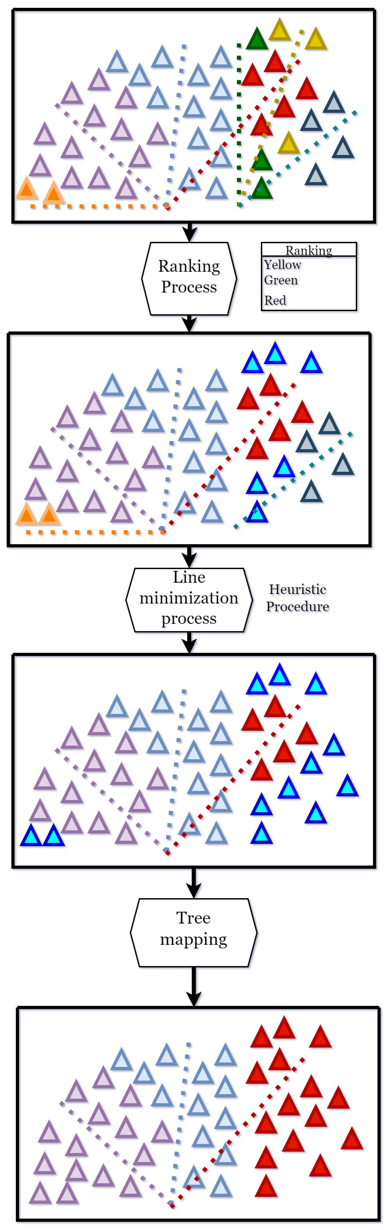
The genetic algorithm is implemented through a two-phase procedure. In the first phase, the evolutionary process identifies candidate lines for extraction, and the fitness function leads to a repair process for the chromosomes of the population. In the second phase, a mathematical model generates the logging cones for each line associated with the best individual selected by the metaheuristic.

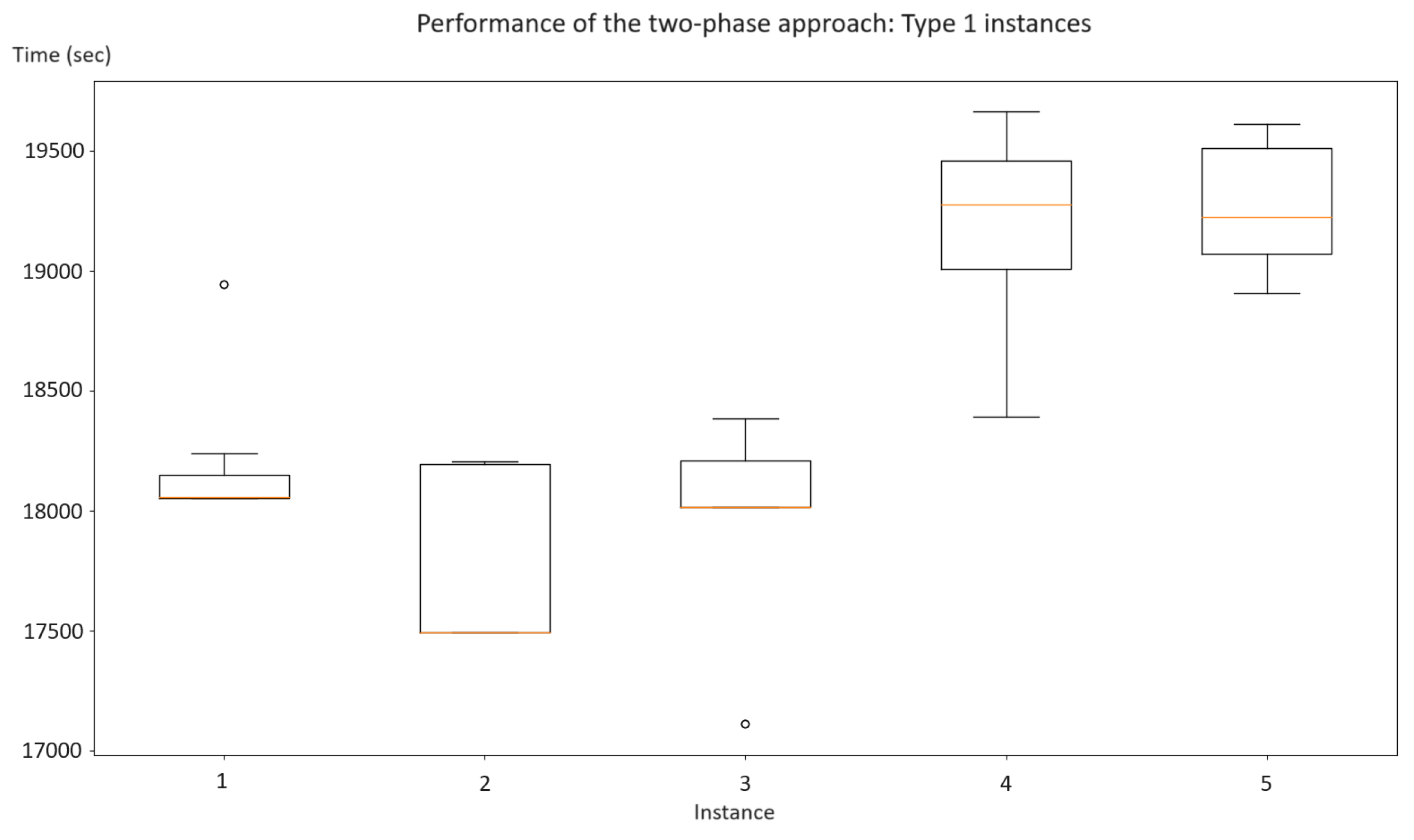
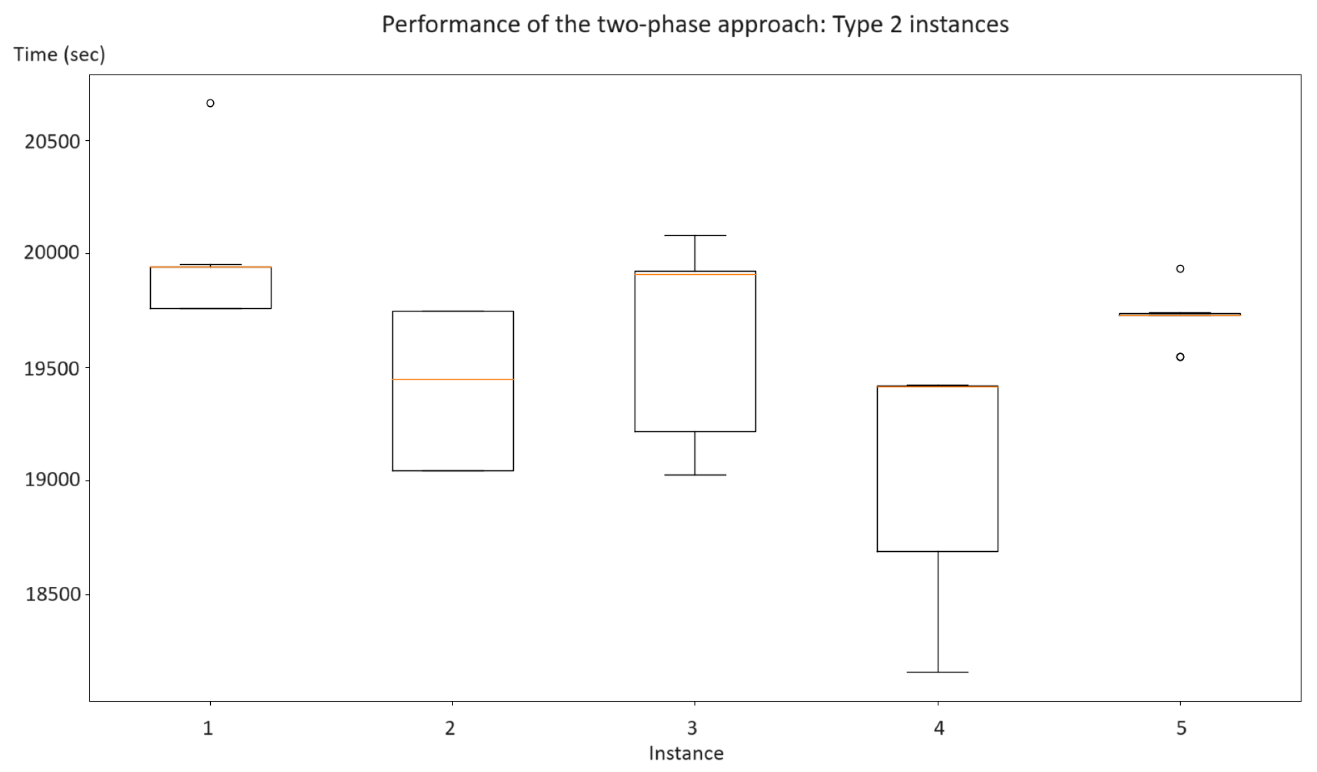
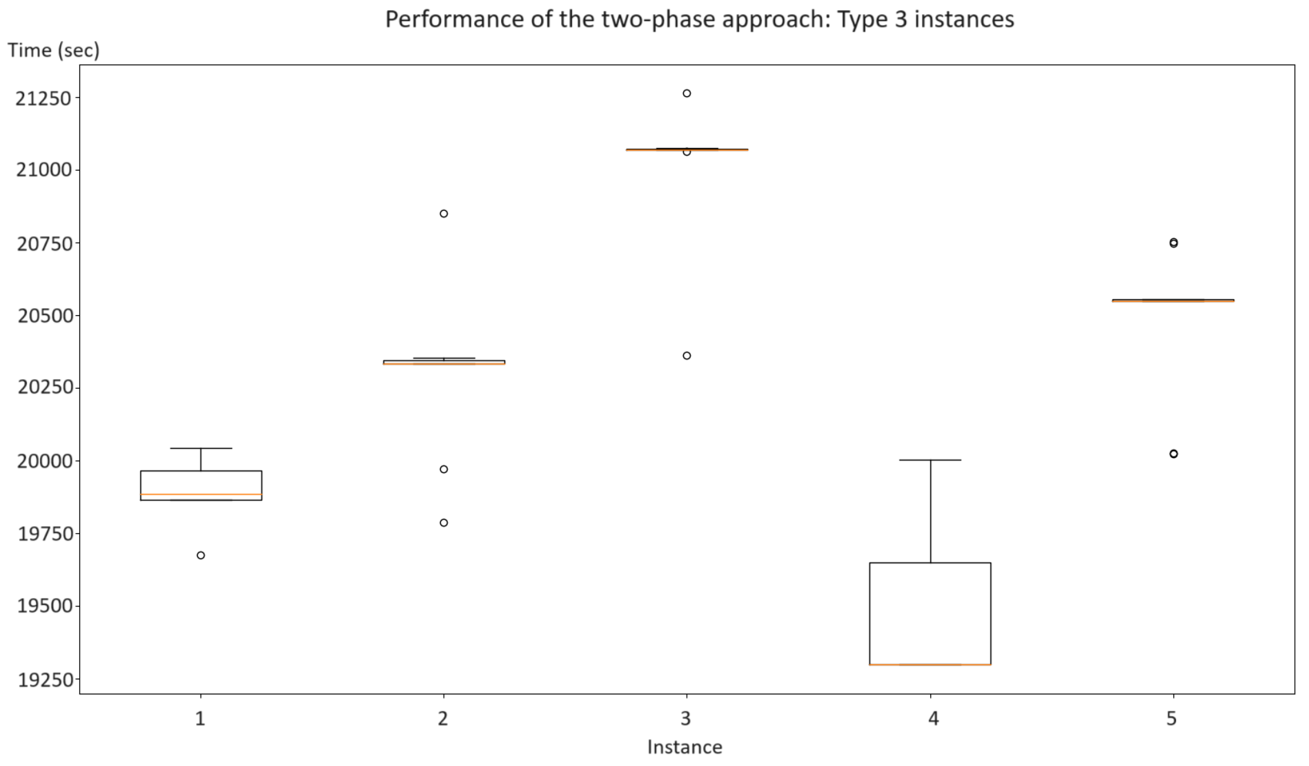
Our findings suggest that the two-phase algorithm offers promising results with a shorter computational time than those provided by a traditional mathematical model. In the cases examined (both randomly generated for this study and real cases from the forestry industry), optimal results were not achieved within an established threshold of 500 s using Gurobi 9.5 and CPLEX 20.0. However, our two-phase approach managed to optimize feasible solutions.

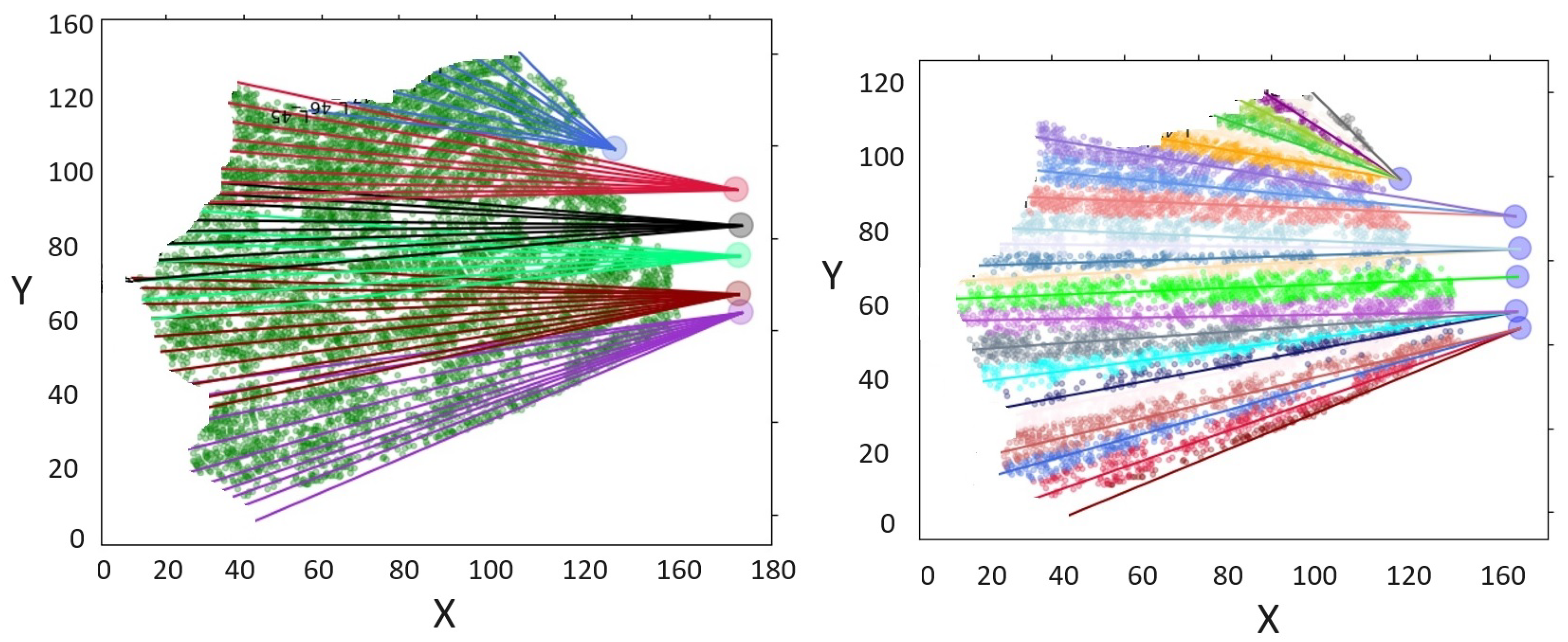
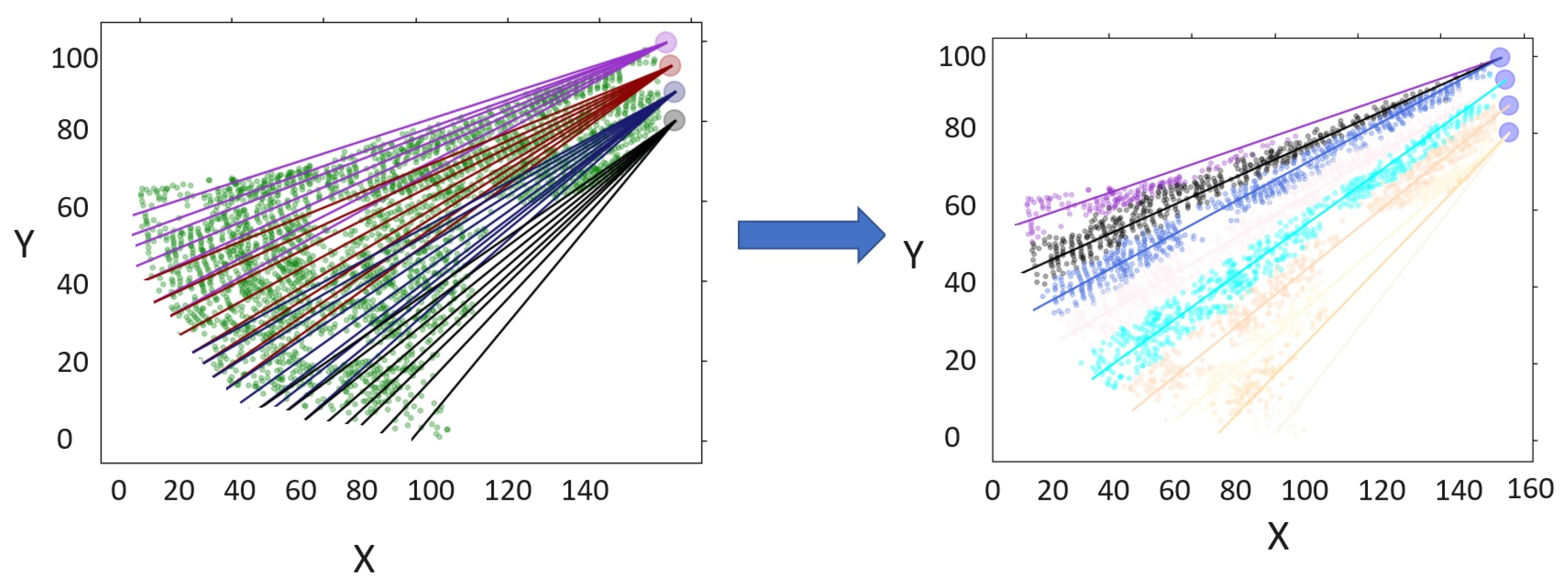
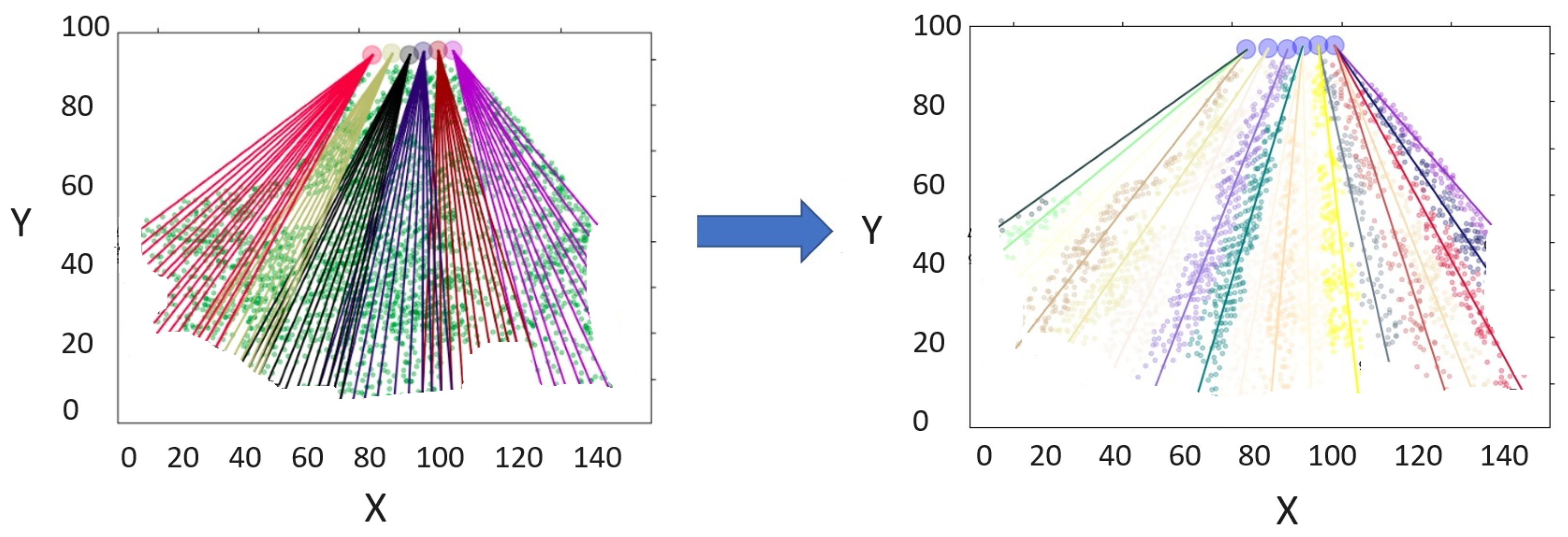
Concerning the topologies addressed in the article, we wish to emphasize that our proposed methodologies are versatile enough to adapt to any given configuration. When observed geometrically, there is a distinct difference between artificial topologies and those derived from real scenarios using drones and Deep Learning. In both situations, our strategies (model and heuristic) have consistently yielded efficient planning times. For future endeavors, we are open to exploring different topological variations and incorporating additional influential factors.

Implementing this approach within companies is entirely feasible. If the focus is on considering extraction and installation times, both the mathematical model and the genetic algorithm approach can be tailored to suit any topology. However, when integrating factors such as fixed expenses, variable expenses, or other input data, the core problem evolves. This necessitates the formulation of new strategies, which could be explored in future research, incorporating insights from existing publications on the topic.

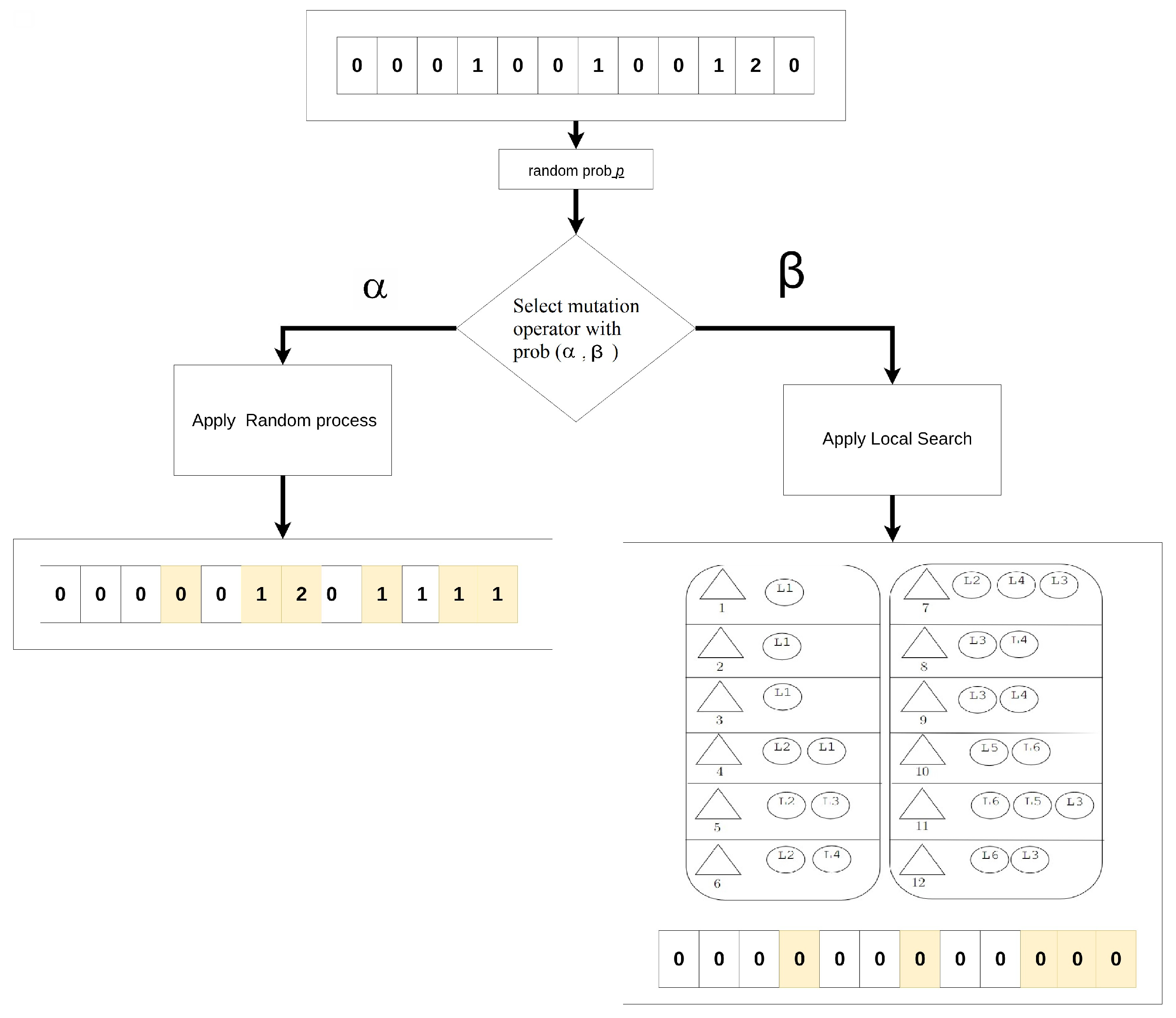
There are several possibilities for future research based on this study. For instance, reducing the problem’s solution space may facilitate obtaining solutions more efficiently. First, a heuristic approach based on Machine Learning could be employed to predict potential lines for harvesting, using various images for training. A second approach is to enhance the proposed genetic algorithm, including a local search after mutation. This process could intensify the chromosomes and allow for better line selection, avoiding local optima. Lastly, it is feasible to consider the application of Lagrangian relaxations to the mathematical model, which could improve bounds during the search process within solvers.

The results of this research are experimental, but they provide a first approach to the integration between Deep Learning and optimization algorithms for the positioning of logging lines. In a first instance, this research addressed the problem in two dimensions, but further experiments should incorporate the topography of the terrain, dasometric variables of the forest, and the operational constraints that this produces in harvesting operations with logging towers.

References

1. Epstein, R.; Weintraub, A.; Sessions, J.; Sessions, B.; Sapunar, P.; Nieto, E.; Bustamante, F.; Musante, H. PLANEX: A system to identify landing locations and access. In Proceedings of the International Mountain Logging and 11th Pacific Northwest Skyline Symposium, Seattle, WA, USA, 10–12 December 2001; pp. 10–12. [Google Scholar]
2. Bont, L.G.; Heinimann, H.R.; Church, R.L. Concurrent optimization of harvesting and road network layouts under steep terrain. Ann. Oper. Res. 2015, 232, 41–64. [Google Scholar] [CrossRef]
3. Dykstra, D.P.; Riggs, J.L. An application of facilities location theory to the design of forest harvesting areas. AIIE Trans. 1977, 9, 270–277. [Google Scholar] [CrossRef]
4. Epstein, R.; Weintraub, A.; Sapunar, P.; Nieto, E.; Sessions, J.B.; Sessions, J.; Bustamante, F.; Musante, H. A combinatorial heuristic approach for solving real-size machinery location and road design problems in forestry planning. Oper. Res. 2006, 54, 1017–1027. [Google Scholar] [CrossRef]
5. Legües, A.D.; Ferland, J.A.; Ribeiro, C.C.; Vera, J.R.; Weintraub, A. A tabu search approach for solving a difficult forest harvesting machine location problem. Eur. J. Oper. Res. 2007, 179, 788–805. [Google Scholar] [CrossRef]
6. Bont, L.; Heinimann, H.R.; Church, R.L. Optimizing cable harvesting layout when using variable-length cable roads in central Europe. Can. J. For. Res. 2014, 44, 949–960. [Google Scholar] [CrossRef]
7. Søvde, N.E.; Løkketangen, A.; Church, R.L.; Oppen, J. A semi-greedy metaheuristic for the European cableway location problem. J. Heuristics 2015, 21, 641–662. [Google Scholar] [CrossRef]
8. Bont, L.G.; Church, R.L. Location set-covering inspired models for designing harvesting and cable road layouts. Eur. J. For. Res. 2018, 137, 771–792. [Google Scholar] [CrossRef]
9. Gallo, R.; Visser, R.; Mazzetto, F. Developing an automated monitoring system for cable yarding systems. Croat. J. For. Eng. J. Theory Appl. For. Eng. 2021, 42, 213–225. [Google Scholar] [CrossRef]
10. Mologni, O.; Marchi, L.; Lyons, C.K.; Grigolato, S.; Cavalli, R.; Röser, D. Skyline tensile forces in cable logging: Field observations vs. software calculations. Croat. J. For. Eng. J. Theory Appl. For. Eng. 2021, 42, 227–243. [Google Scholar] [CrossRef]
11. Knobloch, C.; Bont, L.G. A new method to compute mechanical properties of a standing skyline for cable yarding. PLoS ONE 2021, 16, e0256374. [Google Scholar] [CrossRef]
12. Bont, L.G.; Ramstein, L.; Frutig, F.; Schweier, J. Tensile forces and deflections on skylines of cable yarders: Comparison of measurements with close-to-catenary predictions. Int. J. For. Eng. 2022, 33, 195–216. [Google Scholar] [CrossRef]
13. Holland, J.H. Adaptation in Natural and Artificial Systems: An Introductory Analysis with Applications to Biology, Control, and Artificial Intelligence; MIT Press: Cambridge, MA, USA, 1992. [Google Scholar]
14. Darwin, C. On the Origin of Species, 1859; Routledge: London, UK, 2004. [Google Scholar]
15. Balas, E.; Ho, A. Set covering algorithms using cutting planes, heuristics, and subgradient optimization: A computational study. In Combinatorial Optimization; Springer: Berlin/Heidelberg, Germany, 1980; pp. 37–60. [Google Scholar]
16. Eiben, A.E.; Smith, J.E. Genetic algorithms. In Introduction to Evolutionary Computing; Springer: Berlin/Heidelberg, Germany, 2003; pp. 37–69. [Google Scholar]
17. Ahmad, T.; Ma, Y.; Yahya, M.; Ahmad, B.; Nazir, S.; Haq, A.U. Object detection through modified YOLO neural network. Sci. Program. 2020, 2020, 8403262. [Google Scholar] [CrossRef]
18. Bharati, P.; Pramanik, A. Deep learning techniques—R-CNN to mask R-CNN: A survey. In Computational Intelligence in Pattern Recognition: Proceedings of CIPR 2019; Springer: Singapore, 2020; pp. 657–668. [Google Scholar]
19. Pérez-Carrasco, M.; Karelovic, B.; Molina, R.; Saavedra, R.; Cerulo, P.; Cabrera-Vives, G. Precision silviculture: Use of UAVs and comparison of deep learning models for the identification and segmentation of tree crowns in pine crops. Int. J. Digit. Earth 2022, 15, 2223–2238. [Google Scholar] [CrossRef]
20. López-Ibáñez, M.; Dubois-Lacoste, J.; Pérez Cáceres, L.; Birattari, M.; Stützle, T. The irace package: Iterated racing for automatic algorithm configuration. Oper. Res. Perspect. 2016, 3, 43–58. [Google Scholar] [CrossRef]
Figure 1. Elementary processes for cable logging.
Forests 14 02133 g001
Figure 2. Simple example of a logging cone.
Forests 14 02133 g002
Figure 3. State of the extraction cables.
Forests 14 02133 g003
Figure 4. Example of logging cycles for an extraction cone (in yellow).
Forests 14 02133 g004
Figure 5. Final scenario of extraction cable assignment.
Forests 14 02133 g005
Figure 6. Information structure example.
Forests 14 02133 g006
Figure 7. Representation of an individual.
Forests 14 02133 g007
Figure 8. Feasibility process for a GA individual.
Forests 14 02133 g008
Figure 9. Flowchart for the fitness function.
Forests 14 02133 g009
Figure 10. Crossover Process.
Forests 14 02133 g010
Figure 11. Crossover Process.
Forests 14 02133 g011
Figure 12. Random scenario example.
Forests 14 02133 g012
Figure 13. Utilizing Deep Learning for Forest Monitoring and Optimal Logging Path Determination.
Forests 14 02133 g013
Figure 14. Boxplots for the performance of the two-phase approach: type 1 instances.
Forests 14 02133 g014
Figure 15. Boxplots for the performance of the two-phase approach: type 2 instances.
Forests 14 02133 g015
Figure 16. Boxplots for the performance of the two-phase approach: type 3 instances.
Forests 14 02133 g016
Figure 17. The land before and after the split.
Forests 14 02133 g017
Figure 18. Solution for a Type 1 Instance.
Forests 14 02133 g018
Figure 19. Solution for a Type 2 Instance.
Forests 14 02133 g019
Figure 20. Solution for a Type 3 Instance.
Forests 14 02133 g020