Regional Characteristics of the Climatic Response of Tree-Ring Maximum Density in the Northern Hemisphere

Abstract

The maximum latewood density (MXD) of tree rings can reflect the temperature of the growing season, but the timing of the response differs among regions. We selected 152 maximum latewood density chronologies from the Northern Hemisphere that showed a significant response to temperature. Based on a cluster analysis and the sensitivity of MXD to the monthly mean temperature, the chronologies were classified into six clusters. The clusters showed distinct regional characteristics, and the period and peak month of significant response of the chronologies in each cluster to temperature were different. Spatial synchronization of the MXDs revealed that the two clusters distributed in Europe showed the most consistency and the strongest response to the April–September monthly mean temperature compared with the other clusters. Temperature accounted for more than 40% of the total MXD variance in all clusters, whereas the effect of precipitation was much smaller. In addition to climatic factors, the random effect of the latitude and longitude of sampling sites, elevation, and tree species was a major factor contributing to the variance in MXD in each cluster. Latitude and longitude had the strongest influence among the three random effects, and tree species had the weakest influence, except at high latitudes. The MXD of each cluster showed sensitivity to temperature within a certain interval, with a positive linear response, and the sensitivity interval was greatest at high latitudes. Certain clusters showed a negative linear sensitivity to precipitation. The results provide a reference for studying the climatic threshold of large-scale tree-ring density formation.

1. Introduction

The maximum latewood density (MXD) of tree rings holds considerable potential for global climate reconstruction owing to its greater sensitivity to temperature in the growing season compared with that of tree-ring width (RW) [1]. The MXD has a stronger and more robust climatic signal compared with the signal from tree-ring widths and is reasonably independent of species and site ecology [2]. Based on the existing results of tree-ring density analysis, Schweingruber [3] suggested that the maximum latewood density is suitable for large-scale climate reconstruction. Briffa et al. [4,5] explored in detail the nature of the temperature sensitivity of MXD across the Northern Hemisphere, dividing the network of sampling sites into nine regions according to chronological similarity and demonstrating the dominant common influence of April–September monthly mean temperatures on MXD variability. Frank and Esper [6] observed that the density chronologies explained more of the variance than ring-width chronologies and were significantly correlated with temperature in the April–September period based on a network of 31 MXD and 53 ring-width data sets distributed across the European Alps. However, Büntgen et al. [7] found that the growth response was strongest in the June–September mean temperatures based on 180 larches (Larix decidua Mill.) MXD series from the European Alps. Björklund et al. [8] compared the common variability and climate sensitivity of MXD chronologies for Scots pine (Pinus sylvestris L.) at five sites in the Scandinavian Mountains and determined that the MXD values showed the strongest and most stable response to the temperature from April to August. In addition to temperature, precipitation [9], the self-calibrated Palmer Drought Severity Index (scPDSI) [10], proxies of water availability [11], and other factors influence the MXD chronology in some areas. However, substantially fewer studies have evaluated the effects of such factors than the sensitivity of MXD to summer temperature. Although summer temperature is an important factor influencing the growth sensitivity of the MXD chronology, the months of the strongest responses differ among regions, comprising April–September, April–August, and June–September. Esper et al. [12] observed a good response to spring and autumn temperatures in the south of Spain, which revealed a notable difference from other regions.

Friedrichs et al. [13] used Varimax rotation principal component analysis, Ward’s method, and the average-linkage method to conduct a cluster analysis to effectively classify 46 homogeneous oak (Quercus spp.) tree-ring width chronologies from Central and Western Germany. The different methods resulted in differences in classification for about 20% of the sample sites. In evaluating the trends and uncertainty of warming indicators in Siberia, Esper et al. [14] classified the tree-ring width and density in Siberia. Based on the similarities among the tree-ring chronologies, 78 tree-ring density chronologies in this region were divided into seven clusters. However, the influence of geographical location, elevation, and other factors, as well as the difference in sensitivity to climatic factors, have not been analyzed previously in the classification of MXD data sets from the Northern Hemisphere. Previous chronological classifications were based on the similarity between chronologies. Given that the tree-ring density shows a certain similarity in response to climate, the aims of the present study are (i) to classify tree-ring densities in the Northern Hemisphere by cluster analysis based on the response of MXD chronologies to monthly temperature in different regions; (ii) to identify the differences in response to climatic factors, especially mean temperature and precipitation, among the clustered MXD chronologies; and (iii) to analyze possible reasons for the differences among the clusters. Through classification and feature analysis, we have identified regional differences in tree-ring density and provided a reference for ecological studies and climate reconstruction research across large regions.

2. Materials and Methods

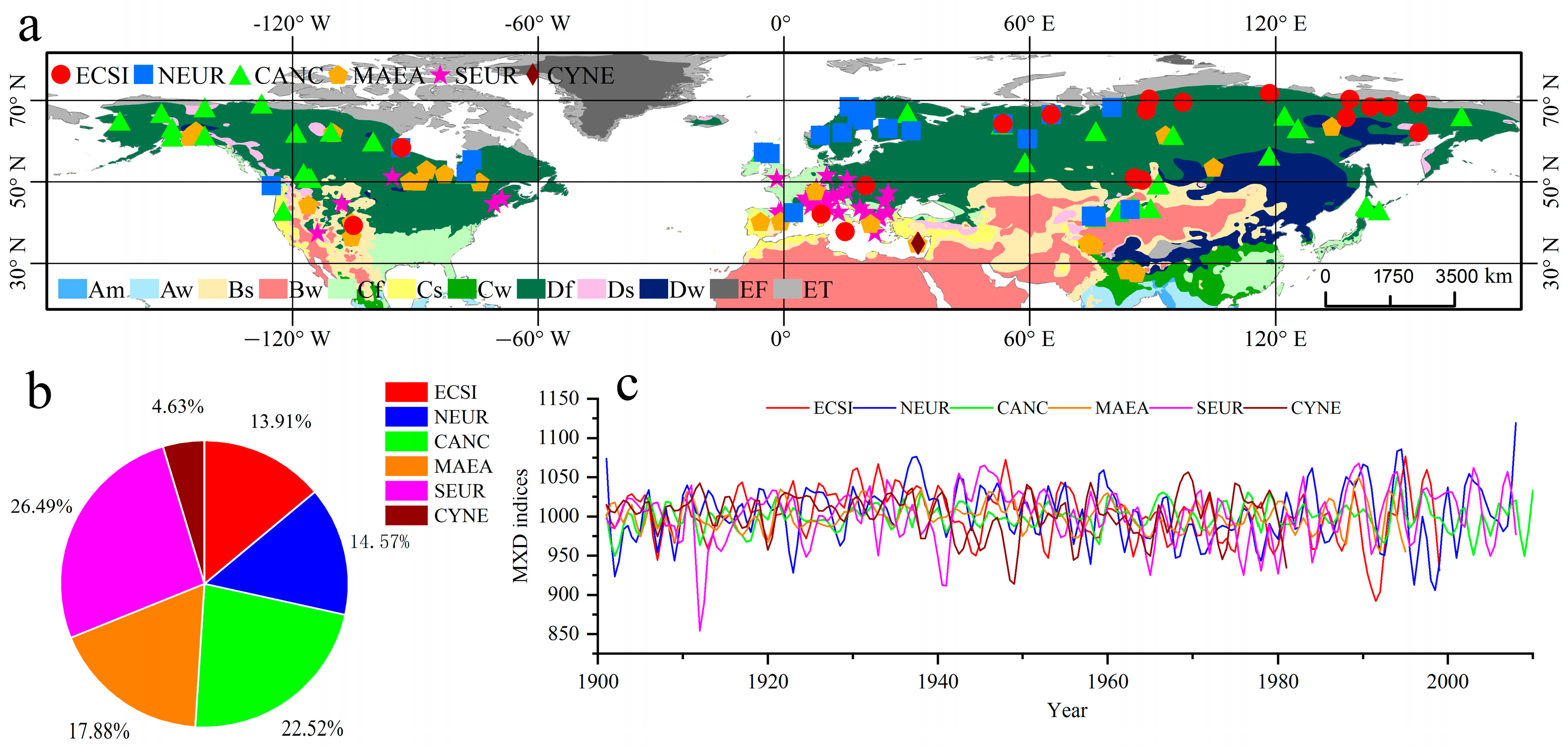
2.1. MXD Chronologies Network

All tree-ring MXD data sets, except the six MXD series for the Tienshan Mountains in China, were sourced from the International Tree-Ring Data Bank (ITRDB; https://www.ncei.noaa.gov/products/paleoclimatology/tree-ring (accessed on 23 October 2023)). Two types of data were obtained from the ITRDB. The first type was the standardized NOAA template chronology, which was used directly in the subsequent analysis. When no standardized NOAA template chronology was available, the MXD raw measurement data, provided by the ITRDB for cross-dating, were downloaded. ARSTAN 4.0 software [15] was used to detrend the series and establish the MXD chronologies. Sampling sites in Europe and North America greatly outnumber data sets from other locations. Given that imbalanced data sets may significantly increase the risk of overfitting [16] and given the uneven geographical distribution of the MXD chronologies, we reduced the number of sampling sites by randomly selecting the 164 MXD chronologies based on their spatial location. In selecting the sites, we considered the spatial distribution and response to climatic factors of the chronologies and excluded certain chronologies that did not show statistically significant correlations with the monthly mean temperature from January to December (p < 0.05). In addition, because there are few MXD chronologies for sites in Central Asia, we chose six new MXD chronologies from high elevations for this region. The sample size of the six chronologies in the Tienshan Mountains was more than 20 trees, and these were cross-dated using COFECHA [17]. In the present analysis, we used (a) cross-dating results of the raw tree-ring width and (b) series individually detrended using ARSTAN with a negative exponential curve or Spline function [15]. Ultimately, we selected 152 chronologies (Table S1) from 170 to generate a MXD network (Figure 1). Based on the Köppen–Geiger climate classification [18], the sampling sites were mostly located in the Cold Without Dry Season (Df), Arid Steppe (BS), Arid Desert (BW), Temperate Without Dry Season (Cf), and Temperate Dry Summer (Cs) climate types. The sites at low and mid latitudes were located in high-altitude mountains. Most of the chronologies used in the dendroclimatic correlation analysis began in 1901, from which the expressed population signal (EPS) [19] value of the chronologies is higher than 0.85. For some chronologies in which the EPS value did not attain 0.85 in 1901, the starting year was based on the year that the EPS was greater than 0.85.

2.2. Climate Data

Dendroclimatic analysis of the tree-ring densities was based on monthly mean temperature and monthly precipitation data from the nearest Climatic Research Unit (CRU) 0.5° × 0.5° grid cell (TS 4.04) [20,21] for each MXD chronology. We obtained the CRU data from the KNMI Climate Explorer (https://climexp.knmi.nl/ (accessed on 23 October 2023)). The CRU data set spans the period 1901–2019, but there are few meteorological stations providing long-term instrumental records in some regions. We screened all meteorological grid data using a 3 year sliding variance window from 1901 and observed that the variance of some gridded data equaled zero in the early portion of the data. Therefore, we discarded the early portion of the records and used data only for the period when the variance was greater than zero.

2.3. Methods

The partitioning around medoids (PAM) clustering method [22] was adopted for cluster analysis of the MXD data. In the PAM method, the algorithm searches the data set and selects k representative objects as the centrotypes (or medoids). After finding a group of centrotypes, the clusters are constructed by assigning each data point to the nearest representative object. Clustering performance was evaluated on the basis of compactness (CP), and the significance of the clustering results was assessed by calculating the p-value with SigClust [23]. The CP is a metric that uses the information inherent in a classified data set [23]. The CP measures the average distance between every pair of data points within the same cluster. The lower the CP value, the better the configuration of the cluster. The SigClust test uses a K-means-based algorithm to calculate a p-value to assess significance in a cluster analysis [24]. This approach sequentially identifies significant splits between groups of clusters and ultimately determines the significance of individual clusters or groups of clusters. Small p-values indicate a superior clustering structure.

We fitted a variance–covariance mixed model (CVM) [25,26] to analyze the spatial synchrony of climate sensitivities among clusters. Based on the diagonal positive-definite matrix structure, CVM calculates the common variance and estimated signal strength parameters for spatial synchrony from the outcome of the models for each cluster. A linear mixed-effects model (LMM) was developed to fit the distribution characteristics of the MXD data in terms of temperature, precipitation, latitude and longitude, elevation, and tree species for each cluster. The LMM is a statistical tool that examines the relationship between climatic factors and explanatory covariates based on the response between the two, taking into account these two types of variations. The coefficient of determination (R²) [27,28], a summary statistic that describes the amount of variance explained, was calculated to quantify the goodness-of-fit of the LMM. Sensitivity analysis of the response of the MXD to meteorological variables was conducted using a treed constant model as a basic Bayesian treed Gaussian process model (TPM) [29,30]. The sensitivity indices of the models were estimated using a Latin hypercube sampling-based method [31], through prediction via one of the TPM models conditional on an observed set of locations, and the sensitivity indices were calculated at each Markov chain Monte Carlo iteration of the TPM fitting. Sensitivity analysis attempts to resolve the natural variability in responses. The indices comprised the main effects and first-order and total sensitivity indices. The main effects were the major contributions of variables to the TPM; the main-effects curves determine the way the variables contribute to the response. The first-order sensitivity is the proportion of the variability in the response attributable to the variable main effects. The total sensitivity measures the residual variance in the conditional expectation and represents all influences connected to a given variable. All statistical analyses were performed using R software version 4.2.0 [32].

3. Results

3.1. Classification of the MXD Chronologies

Briffa et al. determined that most MXD chronologies included a significant positive response to temperature in April–September [4,5]. Therefore, the monthly correlation coefficient from April to September was selected as the observed value, and these sampling points were selected as the sample points. The PAM clustering method was used for classification of the MXD chronologies. The 152 chronologies were classified into 4–9 clusters. The cumulative distribution function (Figure 2a), consensus matrix (Figure 2b), CP, and p-values (

Table 1. Test values for the clustering results.

Test	4	5	6	7	8	9
CP	0.4039	0.3754	0.3609	0.3528	0.3423	0.3519
p	0.0964	0.0055	0.0006	0.0051	0.0055	0.8088

) were calculated to assess the credibility of the six classifications. The cumulative distribution function graph showed that the probability for more than six clusters was more than 0.75 for all consensus index values, and little difference was observed between six and nine clusters, indicating that there were differences in classification among about 25% of the sample points. In contrast, the difference between four and five clusters was more than 40%. Regarding CP, little difference was observed between the six classifications, and values ranged from 0.34 to 0.41. The lowest CP value was observed with eight clusters, but the difference compared with the value with six clusters was 0.018 at most. The lowest p-value (0.0006) was observed for six clusters and indicated extreme significance. Based on the clustering results, six clusters were selected for the final classification. A consensus matrix heatmap of the six clusters was generated (Figure 2b). The heatmap showed there were strong similarities in each classification of the MXD chronologies and the similarity between different clusters was close to zero.

3.2. Characteristics of the Six Clusters

In the final classification of the MXD chronologies, the six clusters showed distinct spatial distribution characteristics. Chronologies in the same cluster did not occur entirely in the same climate zone but were located in relatively concentrated areas. According to the main distribution area of each cluster, the clusters were named from high to low latitude and comprised East and Central Siberia (ECSI), Northern Europe (NEUR), Central Asia and Northwestern Canada (CANC), mid-latitude Asia, Europe, and America (MAEA), Southern Europe (SEUR), and Cyprus and Nepal (CYNE) (Figure 3).

In the ECSI cluster, the sampling sites were mainly concentrated in the high-latitude region of Eastern and Central Siberia in Central Asia, with individual sites distributed in Southern Europe and Central North America. The sites were mostly located in the Cold Without Dry Season (Df) climate type and mountainous areas of the Temperate Dry Summer (Cs) type. A strong correlation between monthly temperature and MXD chronologies in this cluster was observed from June to September. The correlation coefficient for most chronologies was highest in June (Figure 4), with a second peak in September at some sites. No consistency in precipitation among all chronologies in this cluster was observed (Figure 5). Esper et al. [14] reported that the correlation coefficients with temperature in this region from June to August were 0.77–0.89, and the correlation was relatively stable in Central Siberia.

The second cluster at high latitudes was NEUR. Most sites were located in Northern Europe, but some were also distributed in Central Asia and Central Siberia. Similar to the ECSI cluster, most sites were located in the Df climate type. A significant response to the monthly mean temperature was observed from April to August, with the highest correlation coefficient in August. Most sites showed a negative response, with precipitation from July to August. These correlations differed notably from those for the ECSI cluster. The MXD chronology assemblage in Northern Europe showed a correlation coefficient of 0.76 with June and August temperatures [33]. Duthorn [34] noted that the MXD in Northern Finland was most strongly correlated with the temperature in August. The strongest correlation with the monthly mean temperature in the two clusters of high-latitude sites differed: June for ECSI and August for NEUR. The secondary peak value was variable in the NEUR cluster, so the mean monthly coefficient showed only one peak.

The sites in the CANC cluster were located at high- and mid-latitudes, mainly in Central Asia and Northwestern Canada, but some sites on the west coast of the Pacific Ocean were also classified in this cluster. The response characteristics of MXD chronologies to temperature revealed a strong correlation from May to July. Two peaks were observed in May and July, and the July peak was higher in this cluster. A significant effect of precipitation was observed in July and August, which was later than that for temperature.

The MAEA cluster was distributed slightly further to the south than the CANC cluster. The sampling sites in this cluster were mostly located in mid-latitudes and were distributed in Central Asia, South Asia, Central Europe, and Central North America. The cluster was characterized by the influence of temperature in April to May and August to September, and the influence in spring was greater than that in autumn. The influence of precipitation was mainly observed in August, which was slightly earlier or synchronous with the influence of temperature from August to September.

The SEUR cluster included sites mainly located in Southern Europe. The cluster was influenced by temperature from April to May and August to September, but, in contrast to the MAEA cluster, the effect was stronger in August to September than in April to May. Most of the sampling sites were affected by precipitation in July and August, and some in September. The NEUR and SEUR sites in Europe were located in similar taxonomic regions to Briffa’s classification [4,5], but there were significant differences in other clusters.

The CYNE cluster included the fewest sampling sites among all clusters, comprising one site in Nepal in South Asia and several sites in the Mediterranean region. The characteristics of the CYNE cluster were quite different from those from other regions. The correlation with temperature was highest from February to April, and individual sites were also strongly correlated in September. Correlations with precipitation showed no consistency. Similar results have been reported in Southern Spain in the Northern Mediterranean region [9].

Discrepancies in the response of MXD chronologies to temperature among clusters were observed in the period and peak of high correlation. The clusters at high latitudes were unimodal, mid-, and low-latitude clusters were bimodal, and the month of the peak value and the maximum value were not identical. A portion of the MXD chronologies showed a negative response to precipitation late in the growing season.

3.3. Spatial Synchrony between the Six Clusters

We calculated the correlation coefficients and spatial synchronization of the CVM model between the MXD chronologies for all clusters and April–September monthly mean temperatures to compare differences in climate sensitivity among the clusters (Figure 6). The NEUR and SEUR clusters in the European region showed the strongest correlation with April–September temperatures. The correlation coefficients for the NEUR cluster were slightly higher than those for the SEUR cluster. The maximum coefficient value in the NEUR cluster was more than 0.75. Except for the CYNE cluster, no significant difference in sensitivity to temperature was observed among the other three clusters, and the correlation coefficients ranged from 0.2 to 0.6.

The spatial synchronization results showed some differences from the correlation analysis. The SEUR cluster showed the most consistent response to temporal variation in temperature, followed by NEUR. The two clusters were more concentrated than the other clusters, which may be the reason for the high consistency. The ECSI cluster also showed a good response to temperature; the sites in this cluster were mainly located in the high-latitude region. Whereas climate had a greater influence on the spatial variability of the CANC and MAEA clusters, in Europe and Northern Asia, climate warming is leading to temporal coherence in MXD records, whereas in other parts of Asia and the Americas in the Northern Hemisphere, the MXD can represent consistent changes in temperature over a large range. The poor synchronization of MXD responses may be linked to global shifts in the timing of plant phenological events [35] and drought stress at mid-latitudes [36,37], among other factors.

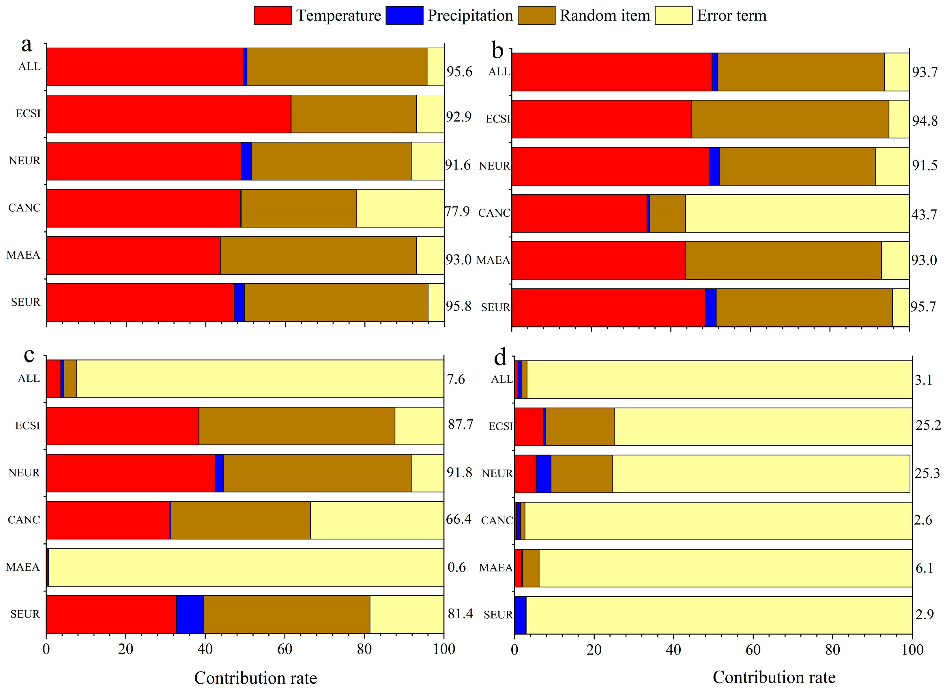
3.4. Influence of Climatic and External Factors

Taking April–September temperature and July–August precipitation as independent variables, latitude and longitude, elevation, and tree species as random variables, and MXD of each cluster as a dependent variable, we established LMMs and calculated R² for each variable to evaluate their influence on each cluster (Figure 7a–d). Because insufficient sites were classified in the CYNE cluster to enable a LMM model to be established, the influence of climatic and external factors on this cluster is not discussed. When the three random variables were included in the LMMs (Figure 7a, ALL), temperature accounted for more than 40% of the MXD variance in all clusters. Among the five clusters, temperature had the greatest influence on ESCI. Precipitation only had a small influence, explaining approximately 1% of the total chronology variation. The random variables contributed to 29%–49% of the MXD variance and had the least influence on the CANC cluster. Temperature, precipitation, and the random variables explained similar proportions of the total variance for the NEUR and SEUR clusters. Precipitation had the strongest influence on these two clusters compared with the other clusters, accounting for approximately 2%–3% of the MXD variation.

In addition, mixed models incorporating the three random variables individually were established (Figure 7b–d). Latitude and longitude were the main contributors to the random effects for all MXD chronologies, explaining about 41.9% of the total variance. Excluding CANC, the latitude and longitude of each cluster explained 39%–49% of the variance in the model. Elevation did not significantly affect the model for all chronologies. The ECSI, NEUR, and SEUR clusters each had a relatively restricted spatial distribution and were significantly affected by elevation, whereas the MAEA cluster was not obviously influenced by elevation. This may be due to the broad geographic distribution of the MAEA cluster, and thus the influence of elevation is on a comparatively small scale. In contrast to the other clusters, elevation was the main influencing factor contributing to the random effects for CANC. This may be because this cluster is mainly distributed in the Cold Without Dry Season (Df) climatic area, and some mid-latitude sites are distributed in the Arid Steppe (Bs) area. The trees in this cluster all grow in cold mountainous regions at elevations above 2200 m at mid-latitudes, and the elevation decreases with an increase in latitude. Therefore, the change in elevation is a major influencing factor for this cluster. Tree species is not an important factor influencing the climatic response of the MXD chronologies in each cluster. However, tree species may contribute more than 15% of the random effect at high latitudes, which indicates that tree species at high latitudes may affect the climate response of the MXD.

3.5. Sensitivity to Climatic Factors

The treed constant model was selected as a basic Bayesian treed Gaussian process model, and the sensitivity of all MXD chronologies and each cluster to the climatic factors was analyzed. The model factors for all chronologies and those of five clusters (ECSI, NEUR, CANC, MAEA, and SEUR) were anomalies of April–September mean monthly temperature and July–August monthly precipitation, and for CYNE anomalies of February–April temperature and precipitation. The main-effect sensitivity to temperature of the MXD chronologies in each cluster resembled a near-linear positive response within a certain temperature range (Figure 8), which was consistent with the results of the correlation analysis, but the sensitivity intensity and sensitivity range differed among each cluster. The range in temperature response sensitivity of all sites was similar to the maximum sensitivity, approximately −1.6 to −1.9 °C, but the slope was low and the intensity was weak. Among all clusters, ECSI and NEUR (comprising sites distributed at high latitudes) showed a greater range in sensitivity to temperature changes than most sites at mid and low latitudes, and the sensitivity intensity was greater at −1.6 to −1.7 °C and −1.9 to −1.6 °C, respectively. The slope of the main-effect sensitivity index for SEUR (comprising sites at mid- and low-latitudes) was the steepest, temperature had the greatest influence on MXD, and the sensitivity range was −1.5 to −0.8 °C. The slope of the main-effect sensitivity index for CANC was much gentler than that of the other clusters, and the sensitivity range was −1.5 to −1.1 °C. The sensitivity range for MAEA was the narrowest among the clusters except CYNE, and the sensitivity range was −1.3 to −0.5 °C. The sensitivity of the MXD chronologies to low temperatures was stronger than the sensitivity to high temperatures at mid and low latitudes.

Regarding the first-order sensitivity index, temperature had the strongest influence on the main effect of NEUR and SEUR, followed by ECSI. The total sensitivity index revealed that the overall sensitivity to temperature and precipitation of MXD was high.

The main-effect sensitivity of MXD chronologies of all clusters to precipitation mainly showed a negative linear response within a certain precipitation interval (Figure 9). The ECSI and CYNE clusters showed no sensitivity to precipitation, which was consistent with the correlation analysis between each cluster and July–August monthly precipitation. The main-effect sensitivity of CANC was predominantly between −140 and −40 mm. The first-order and total sensitivities of this cluster were the highest among all clusters, indicating that the precipitation of the region had a significant influence on the main effect. The MXD responded negatively to precipitation change in the period of low precipitation, whereas change in precipitation had no influence on the MXD in the period of severely low precipitation or when the precipitation was sufficiently high to meet the needs for tree growth. The main-effect sensitivities of the NEUR, SEUR, and MAEA clusters responded to precipitation in the region of zero precipitation anomaly. Their first-order sensitivity index values were low, indicating that precipitation had little influence on the main effect. However, a certain degree of total sensitivity indicated that precipitation may influence MXD sensitivity to temperature, but temperature limitation creates additional sensitivity to precipitation [33].

4. Discussion

4.1. Comparison with Previous Classifications

Although the six clusters in the present classification were fewer than the number resolved by Briff et al. [4,5], there are similarities in the clusters between the two classifications. The NEUR and SEUR clusters were essentially consistent, with the samples located in the same region, and the highest correlation coefficient was between MXD and monthly temperature in August. The correlation coefficient of NEUR from April to August shows a trend of increasing with the month, while the relationship between SEUR and temperature shows a lower peak in April and May than in August [5].

In the Briff et al. classification [4,5], Central and Western Siberia are mainly divided into two clusters, whereas Esper et al. [12] classified the region into eight clusters based on the correlation between chronologies. The present classification divides the sampling points equally into the ESCI cluster. The response characteristics of the ESCI cluster to temperature were more similar to those of Northern Siberia (NSIB) [5], with high correlation coefficients occurring in May.

The CANC cluster includes the clusters of Northwestern North America (NWNA) and Central Asia (CAS) in the Briff et al. classification. The relevant peak months for NWNA are May and August, consistent with CANC, whereas in CAS the peaks are in August.

The Tibetan Plateau (TIBP) and Eastern and Central Canada (ECCA) clusters in the Briff et al. classification were mostly included in the MAEA cluster, and their correlation characteristics with temperature were also consistent. The highest correlation coefficients were in August–September, with April–May representing the secondary peak interval.

The CYNE cluster was not recognized in the classification of Briff et al., possibly because there were insufficient samples with the same temperature response characteristics. We distinguished the CYNE cluster because, in addition to the Cyprus and Nepal regions, the same response characteristics to January–April temperatures were observed in Southern Spain [9], which may represent the characteristics of low-latitude regions where local growth environments (such as differences in elevation) vary.

The present classification exhibited a degree of consistency with that of Briff et al., but some samples with relatively long geographical distances were grouped into a larger cluster based on their response to temperature. The Briff et al. classification places greater emphasis on geographical distribution and consistency between chronologies, whereas the present classification is focused more on the climate response characteristics of MXD.

4.2. Influence of Elevation on Tree-Ring Densities

In addition to geographical location, the elevation of each sampling point is an important factor that affects the temperature response of the MXD chronologies. Buckley et al. [38] observed that the tree-ring width chronologies at high elevation exhibit a strong, direct response to temperature for most growing-season months, whereas the chronologies at low elevation exhibit a weaker, direct response in Western Tasmania, Australia. In British Columbia, Canada, the tree-ring width and MXD chronologies response to climatic factors changed with elevation [39,40]; summer temperature limited tree-ring width at high elevations and MXD at low and high elevations, although the relationship was much stronger at high elevations [39]. In the Tatra Mountains of Slovenia [41], the peak response of MXD to temperature at high elevation is in May and September, which is consistent with the peak for the ESCI cluster. Whereas the low-elevation sampling site only showed a peak response to temperature in May and had a lower correlation coefficient than the high-elevation sampling site. In addition, precipitation in July is an important influencing factor. The mixed-effects model (Figure 7b) also showed that elevation had a significant impact on different clusters in addition to the CANC cluster.

4.3. Threshold and Sensitivity to Climatic Factors

There is a certain physiological range for tree growth to adapt to ecological factors, such as temperature; that is, there is a threshold value [42]. For example, in Northwestern Canada, the critical threshold for tree growth of white spruce at the timberline is 11.3 °C (the temperature in July) [43]. The threshold range for the negative response of Engelmann spruce to July temperature is 13.7–16.8 °C, and when the temperature exceeds 16.8 °C, the tree enters the positive response threshold range [44]. There are reports of similar temperature thresholds in other regions [45,46]. The climatic threshold of tree-ring width is based on the divergence pitfalls [43,44,45,46,47], but no similar study has been undertaken on the climatic threshold of tree-ring density growth. The sensitivity to temperature shown in Figure 8 is a positive linear correlation, whereas precipitation shows a negative correlation in some regions, which is consistent with previous research in the Northern Hemisphere [1,2,3,4,5,48,49,50]. Therefore, the results of the present sensitivity analysis may represent the linear response of tree-ring density to temperature in the study area from April to September. However, because of the presence of common intervals in the samples and differences in tree species (Table S1), further research is needed to determine whether the results of the sensitivity analysis represent climatic thresholds.

5. Conclusions

Taking the monthly correlation coefficient between MXD and April to September as the observation value, 152 MXD chronologies in the Northern Hemisphere were grouped into six clusters. Each cluster had distinct regional characteristics, and the differences among the clusters were mainly the time period of the significant response to temperature and the month of the peak response. Temperature contributed to more than 40% of the MXD variance. The location of the site was the main contributor to the random effect of the mixed-effect model, followed by elevation. Tree species had a small impact at high latitudes. The main-effect sensitivity to temperature of each cluster of MXD chronologies showed a near-linear response within a certain temperature range. High-latitude MXD chronologies had a broader range in temperature sensitivity, and the intensity was greater. The MXD was more sensitive to low temperatures. The MXD of some clusters was not sensitive to changes in precipitation. The main-effect sensitivity of other clusters to precipitation showed a negative linear response within a certain precipitation interval.

References

1. D’Arrigo, R.; Davi, N.; Jacoby, G.; Wilson, R.; Wiles, G. Dendroclimatic Studies: Tree Growth and Climate Change in Northern Forests; John Wiley & Sons Inc: Hoboken, NJ, USA, 2014; p. 88. [Google Scholar]
2. Frank, D.; Esper, J. Temperture reconstruction and comparisons with instrumental data from a tree-ring network for the European Alps. Int. J. Climatol. 2005, 25, 1437–1454. [Google Scholar] [CrossRef]
3. Schweingruber, F.H. Measurement of densitometric properties of wood. In Climate from Tree Rings; Hughes, M.K., Kelly, P.M., Pilcher, J.R., LaMarche, V.C., Eds.; Cambridge University Press: New York, NY, USA, 1982; pp. 8–12. [Google Scholar]
4. Briffa, K.R.; Osborn, T.J.; Schweingruber, F.H.; Jones, P.D.; Shiyatov, S.G.; Vaganov, E.A. Tree-ring width and density data around the Northern Hemisphere (Part 2): Spatio-temporal variability and associated climate patterns. Holocene 2002, 12, 759–789. [Google Scholar] [CrossRef]
5. Briffa, K.R.; Osborn, T.J.; Schweingruber, F.H. Large-scale temperature inferences from tree rings: A review. Glob. Planet Change 2004, 40, 11–26. [Google Scholar] [CrossRef]
6. Frank, D.; Esper, J. Characterization and climate response patterns of a high elevation, multi species tree-ring network in the European Alps. Dendrochronologia 2005, 22, 107–121. [Google Scholar] [CrossRef]
7. Büntgen, U.; Frank, D.C.; Nievergelt, D.; Esper, J. Summer temperature variations in the European Alps, AD 755-2004. J. Clim. 2006, 19, 5606–5623. [Google Scholar] [CrossRef]
8. Björklund, J.A.; Gunnarson, B.E.; Krusic, P.J.; Grudd, H.; Josefsson, T.; Östlund, L.; Linderholm, H.W. Advances towards improved low-frequency tree-ring reconstructions, using an updated Pinus sylvestris L. MXD network from the Scandinavian Mountains. Theor. Appl. Climatol. 2013, 113, 697–710. [Google Scholar] [CrossRef]
9. Rocha, E.; Gunnarson, B.E.; Holzkämper, S. Reconstructing Summer Precipitation with MXD Data from Pinus sylvestris Growing in the Stockholm Archipelago. Atmosphere 2020, 11, 790. [Google Scholar] [CrossRef]
10. Yang, B.; He, M.; Yang, L.; Wang, F.; Ljungqvist, F.C. Pine maximum latewood density in semi-arid northern China records hydroclimate rather than temperature. Geophys. Res. Lett. 2023, 50, e2023GL104362. [Google Scholar] [CrossRef]
11. Pompa-García, M.; Hevia, A.; Camarero, J.J. Minimum and maximum wood density as proxies of water availability in two Mexican pine species coexisting in a seasonally dry area. Trees 2021, 35, 597–607. [Google Scholar] [CrossRef]
12. Esper, J.; Hartl, C.; Tejedor, E.; de Luis, M.; Günther, B.; Büntgen, U. High-Resolution Temperature Variability Reconstructed from Black Pine Tree Ring Densities in Southern Spain. Atmosphere 2020, 11, 748. [Google Scholar] [CrossRef]
13. Friedrichs, D.A.; Neuwirth, B.; Winiger, M.; Löffler, J. Methodologically induced differences in oak site classifications in a homogeneous tree-ring network. Dendrochronologia 2009, 27, 21–30. [Google Scholar] [CrossRef]
14. Esper, J.; Frank, D.; Büntgen, U.; Verstege, A.; Hantemirov, R.M.; Kirdyanov, A.V. Trends and uncertainties in Siberian indicators of 20th century warming. Glob. Chang. Biol. 2010, 16, 386–398. [Google Scholar] [CrossRef]
15. Cook, E.R.; Kairiukstis, L.A. Methods of Dendrochronology Applications in the Environmental Science; Springer: Dordrecht, The Netherlands, 1990; Chapter 1. [Google Scholar]
16. Onel, M.; Kieslich, C.A.; Guzman, Y.A.; Pistikopoulos, E.N. Simultaneous Fault Detection and Identification in Continuous Processes via nonlinear Support Vector Machine based Feature Selection. Comput. Aided Chem. Eng. 2018, 44, 2077–2082. [Google Scholar]
17. Holmes, R.L. Computer-assisted quality control in tree-ring dating and measurement. Tree-Ring Bulletin. 1983, 43, 69–75. [Google Scholar]
18. Peel, M.C.; Finlayson, B.L.; McMahon, T.A. Updated world map of the Köppen-Geiger climate classification. Hydrol. Earth Syst. Sci. 2007, 12, 1633–1644. [Google Scholar] [CrossRef]
19. Wigley, T.M.L.; Briffa, K.R.; Jones, P.D. On the average value of correlated time series, with applications in dendroclimatology and hydrometeorology. J. Appl. Meteorol. Climatol. 1984, 23, 201–213. [Google Scholar] [CrossRef]
20. Harris, I.; Osborn, T.J.; Jones, P.; Lister, D. Version 4 of the CRU TS monthly high-resolution gridded multivariate climate dataset. Sci. Data 2020, 109, 7. [Google Scholar] [CrossRef]
21. Mitchell, T.D.; Jones, P.D. An improved method of constructing a database of onthly climate observations and associated high-resolutiongrids. Int. J. Climatol. 2005, 25, 639–712. [Google Scholar] [CrossRef]
22. Kaufman, L.; Rousseeuw, P.J. Finding Groups in Data: An Introduction to Cluster Analysis; John Wiley & Sons Inc.: New York, NY, USA, 1990; Chapter 1. [Google Scholar]
23. Liu, Y.; Hayes, D.N.; Nobel, A.; Marron, J.S. Statistical Significance of Clustering for High-Dimension, Low-Sample Size Data. J. Am. Stat. Assoc. 2008, 103, 1281–1293. [Google Scholar] [CrossRef]
24. Nguyen, N.; Caruana, R. Consensus Clusterings. In Proceedings of the Third IEEE International Conference on Data Mining, Omaha, NE, USA, 28–31 October 2007; pp. 607–612. [Google Scholar]
25. Shestakova, T.A.; Aguilera, M.; Ferrio, J.P.; Gutierrez, E.; Voltas, J. Unravelling spatiotemporal tree-ring signals in Mediterranean oaks: A variance-covariance modelling approach of carbon and oxygen isotope ratios. Tree Physiol. 2014, 34, 819–838. [Google Scholar] [CrossRef]
26. Shestakova, T.A.; Gutierrez, E.; Kirdyanov, A.V.; Camarero, J.J.; Genova, M.; Knorre, A.A.; Linares, J.C.; Resco de Dios, V.; Sanchez-Salguero, R.; Voltas, J. Forests synchronize their growth in contrasting Eurasian regions in response to climate warming. Proc. Natl. Acad. Sci. USA 2016, 113, 662–667. [Google Scholar] [CrossRef]
27. Nakagawa, S.; Schielzeth, H. A general and simple method for obtaining R2 from generalized linear mixed-effects models. Methods Ecol. Evol. 2013, 4, 133–142. [Google Scholar] [CrossRef]
28. Nakagawa, S.; Johnson, P.C.; Schielzeth, H. The coefficient of determination R2 and intra-class correlation coefficient from generalized linear mixed-effects models revisited and expanded. J. R. Soc. Interface 2017, 14, 20170213. [Google Scholar] [CrossRef]
29. Morris, R.D.; Kottas, A.; Taddy, M.; Furfaro, R.; Ganapol, B.D. A Statistical Framework for the Sensitivity Analysis of Radiative Transfer Models. IEEE Trans. Geosci. Remote Sens. 2008, 46, 4062–4074. [Google Scholar] [CrossRef]
30. Gramacy, R.B. Surrogates: Gaussian Process Modeling, Design and Optimization for the Applied Sciences; Chapman Hall/CRC: Boca Raton, FL, USA, 2020; Chapter 8. [Google Scholar]
31. Saltelli, A. Making best use of model evaluations to compute sensitivity indices. Comput. Phys. Commun. 2002, 145, 280–297. [Google Scholar] [CrossRef]
32. R Core Team. R: A Language and Environment for Statistical Computing; R Foundation for Statistical Computing: Vienna, Austria, 2023; Available online: https://www.R-project.org/ (accessed on 1 May 2023).
33. Esper, J.; Duthorn, E.; Krusic, P. Northern European summer temperature variations over the Common Era from integrated tree-ring density records. J. Quat. Sci. 2014, 29, 487–494. [Google Scholar] [CrossRef]
34. Düthorn, E.; Schneider1, L.; Günther, B.; Gläser, S.; Esper, J. Ecological and climatological signals in tree-ring width and density chronologies along a latitudinal boreal transect. Scand. J. Forest Res. 2016, 31, 750–757. [Google Scholar] [CrossRef]
35. Menzel, A.; Sparks, T.H.; Esterella, N.; Koch, E.; Aasa, A.; Ahas, R.; Alm-kübler, K.; Bissolli, P.; Braslauska, O.; Briede, A.; et al. European phenological response to climate change matches the warming pattern. Glob. Chang. Biol. 2006, 12, 1969–1976. [Google Scholar] [CrossRef]
36. Williams, A.P.; Allen, C.D.; Macalady, A.K.; Griffin, D.; Woodhouse, C.A.; Meko, D.M.; Swetnam, T.W.; Rauscher, S.A.; Seager, R.; Grission-Mayer, H.D.; et al. Temperature as a potent driver of regional forest drought stress and tree mortality. Nat. Clim. Chang. 2013, 3, 292–297. [Google Scholar] [CrossRef]
37. Macias, M.; Andreu, L.; Bosch, O.; Camarero, J.; Gutiérrez, E. Increasing aridity is enhancing silver fir (Abies alba Mill.) water stress in its southwestern distribution limit. Clim. Chang. 2006, 79, 289–313. [Google Scholar] [CrossRef]
38. Buckley, B.; Cook, E.; Peterson, M.; Barbetti, M. Changing temperature response with elevation for Lagarostrobos franklinii in Tasmania, Australia. Clim. Chang. 1997, 36, 477–498. [Google Scholar] [CrossRef]
39. Bernhard, S.; Dobry, J.; Klinka, K. Tree-ring characteristics of subalpine fir (Abies lasiocarpa (Hook.) Nuttv.) in relation to elevation and climatic fluctuations. Ann. Forest Sci. 2000, 57, 89–100. [Google Scholar]
40. Zhang, Q.; Hebda, R. Variation in radial growth patterns of Pseudotsuga menziesii on the central coast of British Columbia, Canada. Can. J. Forest Res. 2004, 34, 1946–1954. [Google Scholar] [CrossRef]
41. Klippel, L.; Büntgen, U.; Konter, O.; Kyncl, T.; Esper, J. Climate sensitivity of high- and low-elevation Larix decidua MXD chronologies from the Tatra Mountains. Dendrochronologia 2020, 60, 125674. [Google Scholar] [CrossRef]
42. Kramer, P.; Kozlowski, T. Physiology of Woody Plants; Academic Press: New York, NY, USA, 1979; pp. 546–627. [Google Scholar]
43. D’Arrigo, R.; Kaufmann, R.; Davi, N. Thresholds for warming-induced growth decline at elevational tree line in the Yukon Territory, Canada. Glob. Biogeochem. Cycles 2004, 18, GB3021. [Google Scholar] [CrossRef]
44. Hart, S.; Laroque, C. Searching for thresholds in climateradial growth relationships of Engelmann spruce and subalpine fir, Jasper National Park, Alberta, Canada. Dendrochronologia 2013, 31, 9–15. [Google Scholar] [CrossRef]
45. Wilmking, M.; Juday, G.; Barber, V. Recent climate warming forces contrasting growth responses of whitespruce at treeline in Alaska through temperature thresholds. Glob. Chang. Biol. 2004, 10, 1724–1736. [Google Scholar] [CrossRef]
46. Peltier, D.; Ogle, K. Tree growth sensitivity to climate is temporally variable. Ecol. Lett. 2020, 23, 13575. [Google Scholar] [CrossRef]
47. Esper, J.; Frank, D. Divergence pitfalls in tree-ring research. Clim. Chang. 2009, 94, 261–266. [Google Scholar] [CrossRef]
48. Grudd, H. Torneträsk tree-ring width and density AD 500–2004: A test of climatic sensitivity and a new 1500-year reconstruction of north Fennoscandian summers. Clim. Dynam. 2008, 31, 843–857. [Google Scholar] [CrossRef]
49. Cerrato, R.; Salvatore, M.C.; Gunnarson, B.E.; Linderholm, H.W.; Carturan, L.; Brunetti, M.; De Blasi, F.; Baroni, C. A Pinus cembra L. tree-ring record for late spring to late summer temperature in the Rhaetian Alps, Italy. Dendrochronologia 2019, 53, 22–31. [Google Scholar] [CrossRef]
50. Nagavciuc, V.; Roibu, C.-C.; Ionita, M.; Mursa, A.; Cotos, M.-G.; Ionel, P. Different climate response of three tree ring proxies of Pinus sylvestris from the Eastern Carpathians, Romania. Dendrochronologia 2019, 54, 56–63. [Google Scholar] [CrossRef]
Figure 1. Location of the maximum latewood density chronologies in the Northern Hemisphere. The Köppen–Geiger climate classification map was derived from Peel et al. [18]. Climate types: Am = Tropical Monsoon; Aw = Tropical Savannah; Bs = Arid Steppe; Bw = Arid Desert; Cf = Temperate Without Dry Season; Cs = Temperate Dry Summer; Cw = Temperate Dry Winter; Df = Cold Without Dry Season; Ds = Cold Dry Summer; Dw = Cold Dry Winter; EF = Polar Frost; ET = Polar Tundra.
Forests 14 02122 g001
Figure 2. (a) Cumulative distribution function graph. (b) Consensus matrix heatmap of the six clusters. ECSI = East and Central Siberia; NEUR = Northern Europe; CANC = Central Asia and Northwestern Canada; MAEA = mid-latitude Asia, Europe, and America; SEUR = Southern Europe; CYNE = Cyprus and Nepal.
Forests 14 02122 g002
Figure 3. (a) Distribution of the six clusters and all MXD sampling sites in the Northern Hemisphere. Clusters: ECSI = East and Central Siberia; NEUR = Northern Europe; CANC = Central Asia and Northwestern Canada; MAEA = mid-latitude Asia, Europe, and America; SEUR = Southern Europe; CYNE = Cyprus and Nepal. (b) Pie chart of the cluster proportions. (c) Weighted average line for each cluster based on correlation coefficients.
Forests 14 02122 g003
Figure 4. Line and box plots of the correlation coefficient between MXD chronologies and monthly mean temperature in each cluster. The dotted line indicates the period of strong mean correlations in each cluster.
Forests 14 02122 g004
Figure 5. Lines and boxplots of the correlation coefficient between MXD chronologies and monthly precipitation for each cluster. The dotted line indicates the period of strong mean correlations in each cluster.
Forests 14 02122 g005
Figure 6. (a) Violin plot of correlation coefficients and (b) spatial synchrony between MXD chronologies and April–September mean monthly temperature.
Forests 14 02122 g006
Figure 7. Contribution rate of factors in the mixed-effect models. The fixed-effect factors were April–September mean monthly temperature and July–August monthly precipitation. The random-effect factors were: (a) latitude and longitude, elevation, and tree species; (b) latitude and longitude; (c) elevation; and (d) tree species. The values on the right of each plot are R2 values for each mixed model.
Forests 14 02122 g007
Figure 8. Main effects, first-order, and total sensitivity indices for temperature of Bayesian treed Gaussian process models. The independent variable for the ECSI, NEUR, CANC, MAEA, SEUR, and ALL clusters is July–August monthly precipitation, and that for the CYNE cluster is February–April mean monthly temperature.
Forests 14 02122 g008
Figure 9. Main effects, first-order, and total sensitivity indices for precipitation of Bayesian treed Gaussian process models. The independent variable for the ECSI, NEUR, CANC, MAEA, SEUR, and ALL clusters is July–August monthly precipitation, and that for the CYNE cluster is February–April monthly precipitation.
Forests 14 02122 g009