Article

Evaluation of the Community Land Model-Simulated Specific Leaf Area with Observations over China: Impacts on Modeled Gross Primary Productivity

1
Key Laboratory of Ecosystem Network Observation and Modeling, Institute of Geographic Sciences and Natural Resources Research, Chinese Academy of Sciences, Beijing 100101, China
2
National Ecosystem Science Data Center, Beijing 100101, China
3
University of Chinese Academy of Sciences, Beijing 100049, China
4
College of Resources and Environment, University of Chinese Academy of Sciences, Beijing 100190, China
5
School of Earth System Science, Tianjin University, Tianjin 300072, China
6
Chinese Academy of Meteorological Sciences, Beijing 100081, China
*
Author to whom correspondence should be addressed.
Forests 2023, 14(1), 164; https://doi.org/10.3390/f14010164
Submission received: 22 December 2022 / Revised: 9 January 2023 / Accepted: 10 January 2023 / Published: 16 January 2023
(This article belongs to the Special Issue Modelling Forest Ecosystems)

Abstract

:
Specific leaf area (SLA) is a key leaf functional trait associated with the ability to acquire light. Substantial variations in SLA have not been well described in the community land model (CLM) and similar terrestrial biosphere models. How these SLA variations influence the simulation of gross primary productivity (GPP) remains unclear. Here, we evaluated the mismatch in SLA between the CLM4.5 and observed data collected from China and quantified the impacts of SLA variation calculated from both observations and the default values across seven terrestrial biosphere models on modeled GPP using CLM4.5. The results showed that CLM4.5 tended to overestimate SLA values at the top and gradient of the canopy. The higher default SLA values could cause an underestimation of the modeled GPP by 5–161 g C m−2 yr−1 (1%–7%) for temperate needleleaf evergreen tree (NET), temperate broadleaf deciduous tree (BDT), and C3 grass and an overestimation by 50 g C m−2 yr−1 (2%) for temperate broadleaf evergreen tree (BET). Moreover, the observed SLA variation among species ranged from 21% to 59% for 14 plant functional types (PFTs), which was similar to the variation in default SLA values across models (9%–60%). These SLA variations would lead to greater changes in modeled GPP by 7%–19% for temperate NET and temperate BET than temperate BDT and C3 grass (2%–9%). Our study suggested that the interspecific variation in SLA and its responses to environmental factors should be involved in terrestrial biosphere models; otherwise, it would cause substantial bias in the prediction of ecosystem productivity.

1. Introduction

Plant functional traits are core attributes that reflect important ecological strategies in plants [1,2]. As a leaf functional trait, specific leaf area (SLA) is an important indicator of resource trade-off strategies under environmental changes, which determines the ability of a plant to capture light [3,4,5]. Specific leaf area refers to the leaf area per unit of leaf biomass, which is of great significance for vegetation photosynthesis and ecosystem productivity [6,7].
Substantial variation in SLA exists among plant functional types (PFTs) (e.g., needleleaf evergreen tree and broadleaf deciduous tree) and species for a given PFT. Numerous surveys have shown that SLA varies with different plant functional types (PFTs), following a general pattern of herb > shrub > tree, broadleaved > coniferous, and deciduous > evergreen [8,9,10]. Moreover, plant SLA among different species also shows significant variability. Based on the TRY Global Plant Traits Database, the variation coefficients (CV) of SLA data within the same PFT reach up to 23%–78% [9]. Such a large interspecific variation in SLA for a given PFT has also been reported in China and other regions [11]. For example, Liu et al. investigated plant SLA for 76 natural communities in China, the CV of different forest types ranged from 40% to 60%, and those of herb and shrub were 66% and 57%, respectively [12]. In the study by Reich et al., the CV of SLA was 34.3% for the broadleaf deciduous tree and 44.7% for the needleleaf evergreen tree based on field data across sites in the USA [13]. However, such a leaf trait diversity has not been well described in state-of-the-art terrestrial biosphere models.
In most terrestrial biosphere models, vegetation is grouped into different plant functional types with specific plant functional traits. This simple scheme is an effective way to characterize the functional diversity of ecosystems on the regional and global scales [14,15]. As for the expression of SLA, each plant functional type has a corresponding mean SLA value that can be calculated from observations. Few models consider the vertical variability of SLA within the canopy as in the community land model (CLM) [16,17]. Nevertheless, the default trait value settings for each PFT in different terrestrial biosphere models vary with each other and are different from the observations made at multiple spatial scales [9,18]. The uncertainties in plant trait parameters would considerably impact the prediction of vegetation productivity [19,20]. For example, the uncertainties in leaf longevity resulted in a greater than 30% change in vegetation biomass for temperate broadleaf evergreen tree in the Lund–Potsdam–Jena model [21]. However, how the SLA variation within each plant functional type influences the terrestrial gross primary productivity (GPP) simulation still remains unclear.
The objectives of this study were to investigate (1) the mismatch between simulated SLA in the CLM (version 4.5) and observed data for 1056 species in China and the differences in default SLA values across seven terrestrial biosphere models and (2) how the variation in SLA values influences GPP modeling for different ecosystems. Here, we first compared the default SLA values in the CLM4.5 model with published plant SLA observation data collected in China from 2005 to 2022. The variation in observed SLA data for each PFT and the difference in default parameter values of SLA in seven terrestrial biosphere models (i.e., BEPS, JULES, Hybrid, BIOME-BGC, SiBCASA, CLM4.5, and IBIS) were then quantified. Taking three forest ecosystems and one grassland ecosystem as an example, we finally quantified the uncertainties in modeled GPP caused by the mismatch in SLA between the mean observed values and original default values in CLM4.5, and the SLA variations among species and across different models for a given PFT.

2. Materials and Methods
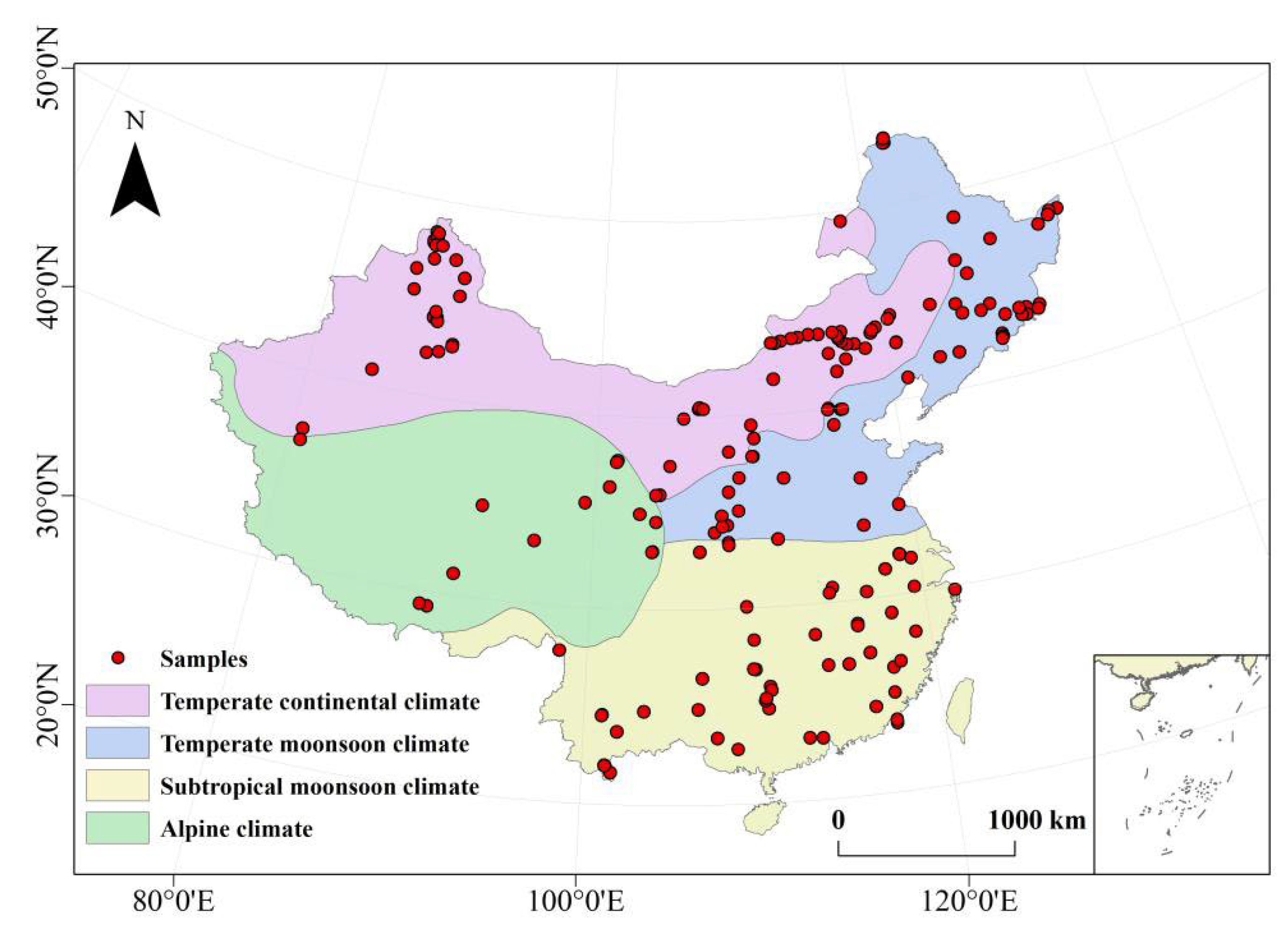
2.1. Data

We collected 2632 records of observed specific leaf area (SLA) data for 1056 species from published papers during 2005–2020 by searching for keywords (i.e., leaf traits, specific leaf area, leaf mass per area, China) in the Web of Science and the China National Knowledge Infrastructure. SLA values estimated from models were excluded. These SLA data were distributed in different climates zones (Figure 1).
According to the plant functional types setting in the CLM4.5 model and observations in China, we statistically analyzed the SLA data for 15 plant functional types (PFTs), including temperate and boreal needleleaf evergreen tree (temperate and boreal NET), boreal needleleaf deciduous tree (boreal NDT), tropical and temperate broadleaf evergreen tree (tropical and temperate BET), tropical and temperate and boreal broadleaf deciduous tree (tropical and temperate and boreal BDT), temperate broadleaf evergreen shrub (temperate BES), temperate and boreal broadleaf deciduous shrub (temperate and boreal BDS), C3 grass, C4 grass, and rainfed crop (Table S1). Here, we combined C3 arctic grass and C3 grass with the same default SLA value in the CLM4.5 model into one plant functional type. We used the coefficient of variation (CV) to quantify the variation in SLA among species within the same plant functional type.
The default SLA parameter values for plant functional types were collected from seven state-of-the-art terrestrial biosphere models, including Boreal Ecosystems Productivity Simulator (BEPS), the Joint UK Land Environment Simulator (JULES), Hybrid model, Biome Biogeochemical model (BIOME-BGC), Simple Biospher and Carnegie-Ames-Stanford Approach model (SiBCASA), Community Land Model (CLM4.5), and Integrated Biosphere Simulator (IBIS) [18,22,23,24,25,26]. Considering the differences in PFT assignment among the seven models, we just compared the differences in default SLA values among the models for eight plant functional types, i.e., NET, NDT, BDT, BET, BES, BDS, grass, and crop). For the models with subgroups for each of the eight PFTs, we used the average default SLA values of all subgroups.
Half-hourly climate data (i.e., downwelling short-wave radiation (W m−2), downwelling long-wave radiation (W m−2), air temperature (K), precipitation (mm s−1), surface pressure (Pa), relative humidity (%), and wind speed (m s−1)) at four ChinaFLUX sites (http://www.nesdc.org.cn/ accessed on 15 June 2022) were collected to drive the CLM4.5 model. The four sites included Qianyanzhou subtropical coniferous forest (QYZ), Changbaishan temperate broadleaved Korean pine mixed forest (CBS), Dinghushan subtropical evergreen coniferous forest (DHS), and Haibei alpine shrub-meadow (HBG). The CBS temperate broadleaf deciduous forest is an old growth forest in northeastern China. The HBG is a typical grassland site in the Qinghai–Tibet Plateau. QYZ and DHS are two evergreen forests in southern China. A brief description of the sites’ characteristics is listed in Table 1.
Missing climate data were filled in using observations from meteorological stations at the same site in the Chinese Ecosystem Research Network (CERN) (http://ww.cnern.org.cn/ accessed on 25 June 2022). A seven-day running mean diurnal cycle was used under the absence of station data. Other input data (e.g., plant functional type, soil depth, and texture) were also collected at these sites. More details were given by Zhang et al. [27].

2.2. Model

CLM4.5 is a state-of-the-art land surface process model in the Community Earth System Model (CESM1.2), which couples terrestrial biogeophysical processes, biogeochemical processes, and hydrological processes. CLM models have been evaluated widely for carbon fluxes and pools, evapotranspiration, leaf area index, land water storage, and soil moisture at different temporal and spatial scales [28,29,30,31,32,33,34]. The CLM4.5 model showed a good performance when simulating GPP at the above four sites [27].
In CLM4.5, photosynthesis in C3 and C4 plants was simulated based on the models of Farquhar et al. and Collatz et al. [35,36], respectively. Leaf net photosynthesis ( A n ) is defined as follows:
A n = min A c , A j , A e R d
where A c is the RuBP carboxylase (Rubisco) limited rate of carboxylation ( μ mol   CO 2 m 2   s 1 ), A j is the maximum rate of carboxylation allowed by the capacity to regenerate RuBP ( μ mol   CO 2   m 2   s 1 ), A e is the product-limited rate of carboxylation for C3 plants and the PEP carboxylase-limited rate of carboxylation for C4 plants, and R d is the leaf dark respiration rate ( μ mol   CO 2   m 2   s 1 ).
Photosynthesis is calculated separately for sunlit and shaded leaves to scale up carbon flux from the leaf to canopy levels.
A c = A sun LAI sun + A shade LAI shade
where A sun and A shade are the photosynthesis for sunlit and shaded leaves (CO2 m−2 s−1), LAI shade is the sunlit and shaded leaf area indices, and A c is expressed as follows:
A c = V cmax c i Γ * c i + K c 1 + o i / K o          for   C 3   plants V cmax    for   C 4   plants
where V cmax is the maximum rate of carboxylation ( μ mol   m 2   s 1 ); c i is the internal leaf CO2 partial pressure (Pa); o i is the O2 partial pressure (Pa); K c and K o are the Michaelis–Menten constants (Pa) for CO2 and O2, respectively; and Γ * is the CO2 compensation point (Pa).
V cmax depends on temperature and is calculated from the value at 25 °C ( V cmax 25 ). V cmax 25 varies with foliage nitrogen concentration and specific leaf area.
V cmax 25 = N a F LNR F NR a R 25
where N a is the area-based leaf nitrogen concentration (g N m−2 leaf area), F LNR is the fraction of leaf nitrogen in Rubisco (g N in Rubisco g−1 N), F NR is the mass ratio of total Rubisco molecular mass to nitrogen in Rubisco (g Rubisco g−1 N in Rubisco), and a R 25 is the specific activity of Rubisco ( μ mol   CO 2   g 1   Rubiscos 1 ). N a is calculated from the mass-based leaf nitrogen concentration and specific leaf area:
N a = 1 CN L SLA 0
where CN L is the leaf carbon-to-nitrogen ratio (g C g−1 N) and SLA 0 is specific leaf area at the canopy top (m2 leaf area g−1 C).
The vertical variability in SLA within the canopy was simulated by a linear function of SLA and the canopy depth as follows:
SLA x = SLA 0 + mx
where SLA 0 is a fixed value of SLA at the top of the canopy (m2 g−1), m is a linear slope coefficient, and x is the canopy depth expressed as overlying leaf area index (m2 overlying one-sided leaf area m2 ground area). SLA 0 and m are both assumed to vary with plant functional type. More details of the CLM4.5 model can be found in Oleson et al. and Thornton et al. [25,37]. Although the leaf nitrogen content and Vcmax25 are updated from static values in CLM4.5 to variates simulated by the leaf utilization of nitrogen for the assimilation (LUNA V1.0) model in the new version of the CLM model (CLM5.0), the quantification of SLA and related main processes in simulating photosynthesis remain the same as in CLM4.5 [38,39].

2.3. Analysis of the Impact of SLA Variation on Gross Primary Productivity

We conducted six model experiments to examine the impacts of SLA variation on gross primary productivity at the QYZ (temperate NET), CBS (temperate BDT), DHS (temperate BET), and HBG (C3 grassland) sites. Different SLA values were used in the six experiments. The default SLA values in the CLM4.5 model (p0) were used in experiment S1. In experiment S2, we used the mean value of the observed SLA data collected in this study for each PFT (pobs). In experiments S3 and S4, we added the observed SLA variation to the mean SLA value used in experiment S2 (i.e., pobs − SDobs and pobs + SDobs, respectively). In experiments S5 and S6, the variation in default SLA values across the models was added to the mean default SLA values (pmod) of the seven terrestrial biosphere models (i.e., pmod − SDmod and pmod + SDmod, respectively).
For each model experiment, we first ran the CLM4.5 model to obtain the initial values of the state variables under equilibria using a two-stage spin-up approach. The first stage of spin-up followed the accelerated decomposition for 600 years; then, a normal decomposition was implemented for 200 years, with a repeating cycle of 6 years (2003–2008) with dynamic meteorological forcing and constant land use types, CO2 concentration (284 ppmv), and N deposition (0.5 g N m−2 yr−1) at the pre-industrial level. A transient run was operated from 1850 to 2008 after reaching equilibrium. The CO2 concentration and N deposition data for the four sites were downloaded from the global dataset described in Thornton et al. [37].
The relative changes in gross primary productivity (GPP), RuBP-limited photosynthesis rate (Ac), and leaf area index (LAI) in model experiments S3 and S4 were compared with the results in experiment S2 (Equation (7)). The relative changes in GPP, Ac, and LAI in model experiments S4 and S5 were compared with the results in experiment S6 (Equation (8)).
R 1 = MAX ( M S 3 M S 2 M S 2 , M S 4 M S 2 M S 2 ) × 100 %
R 2 = MAX ( M S 5 M S 1 M S 1 , M S 6 M S 1 M S 1 ) × 100 %
where R1 and R2 are the relative changes in modeled GPP, Ac, and LAI caused by SLA variation from observations and models and M S i is the model outputs of GPP, Ac, and LAI in model experiments S1, S2, S3, S4, S5, and S6.

3. Results

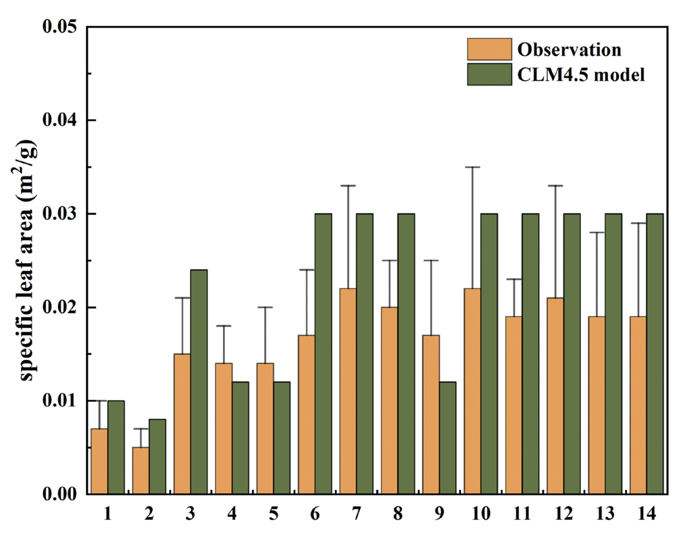
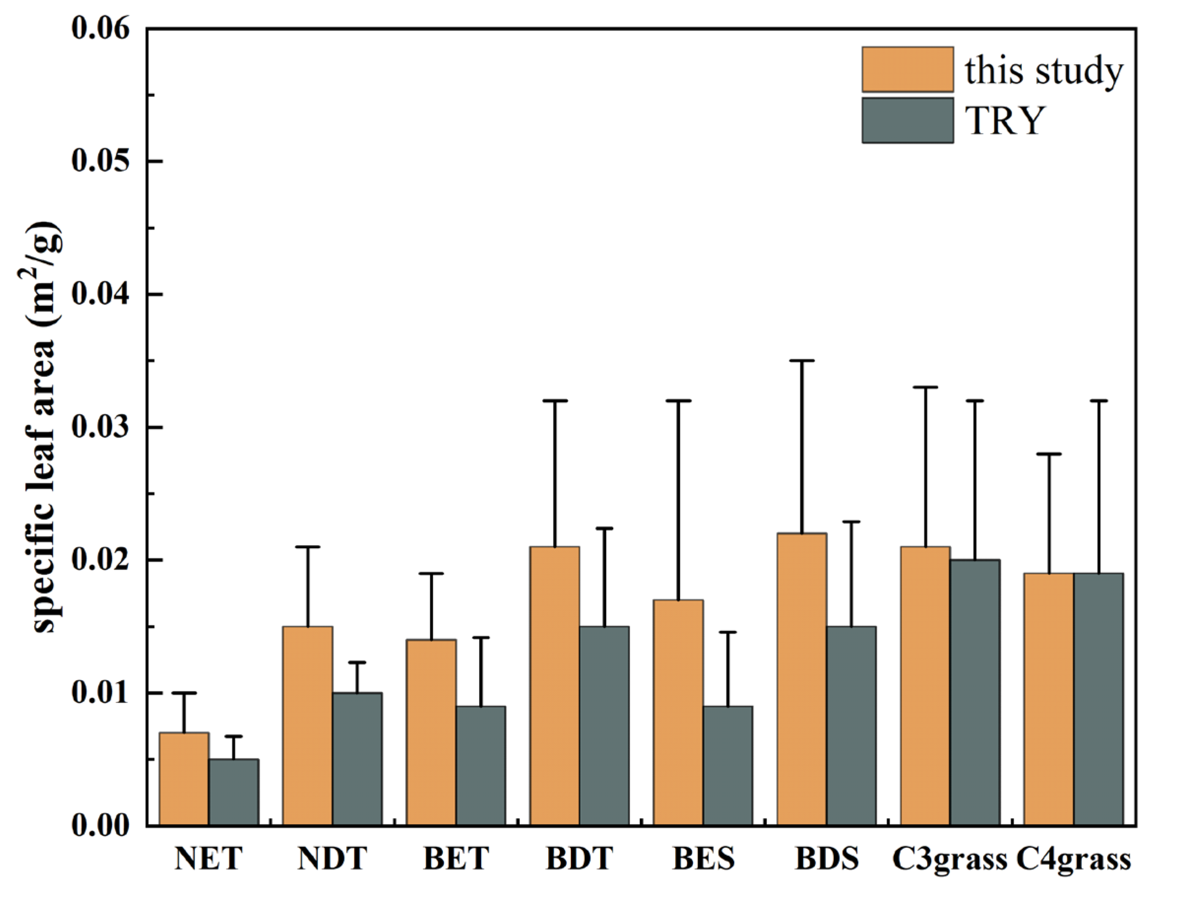
3.1. Comparison of SLA between the CLM Model and Observations over China

We compared the SLA of mean observed values in China with default values in the CLM4.5 for 14 plant functional types (PFTs), as shown in Figure 2. The default SLA values were shown as broadleaf deciduous tree (BDT) > needleleaf deciduous tree (NDT) > broadleaf evergreen tree (BET) > needleleaf evergreen tree (NET), and broadleaf deciduous shrub (BDS) > broadleaf evergreen shrub (BES), which were consistent with the observations. However, the CLM4.5 model overestimated SLA values by 0.009 m2/g on average for most PFTs, except for tropical BET, temperate BET, and temperate BES. The positive bias of the default SLA values was highest (0.013 m2/g) in tropical BDT and lowest (0.003 m2/g) in temperate NET. By contrast, the CLM4.5 model underestimated the SLA values by 0.002 m2/g in tropical BET and temperate BET and by 0.005 m2/g in temperate BES.
We also evaluated the vertical gradients in simulated SLA varying with light from the bottom to top of the canopy for temperate BDT, temperate NET, and temperate BET in CLM4.5 (Figure 3). Compared with the observations, the CLM4.5 model overvalued canopy gradients of SLA in temperate BDT (Figure 3a) and temperate NET (Figure 3b), mainly because of the overestimation of SLA values at the top canopy. Specifically, the decrease of 0.016 m2/g in simulated SLA in temperate BDT was larger than the mean reduction of 0.014 m2/g observed for Phellodendron amurense Rupr., Fraxinus mandschurica Rupr., and Juglans mandshurica Maxim. when light intensity increased from 15% to 100%. For temperate NET, the simulated SLA decreased by 0.005 m2/g as light intensity increased from 15% to 100%, which was the same as the observed change in Picea asperata Mast., but larger than the slight reduction of 0.002 m2/g for Pinus koraiensis Siebold & Zucc. In addition, the simulated vertical gradients in SLA in temperate BET were within the range of SLA values observed for the three species (Figure 3c). However, the response of simulated SLA value was underestimated by 0.006 m2/g compared with the observed variation for Ficus tinctoria G.Forst. and Serianthes nelsonii Merr. when light intensity varied from 0 to 100%. Moreover, the CLM4.5 model ignored the interspecific diversity of plants in the response of SLA to light gradients, especially for the temperate BDT (Figure 3a) and BET (Figure 3c).

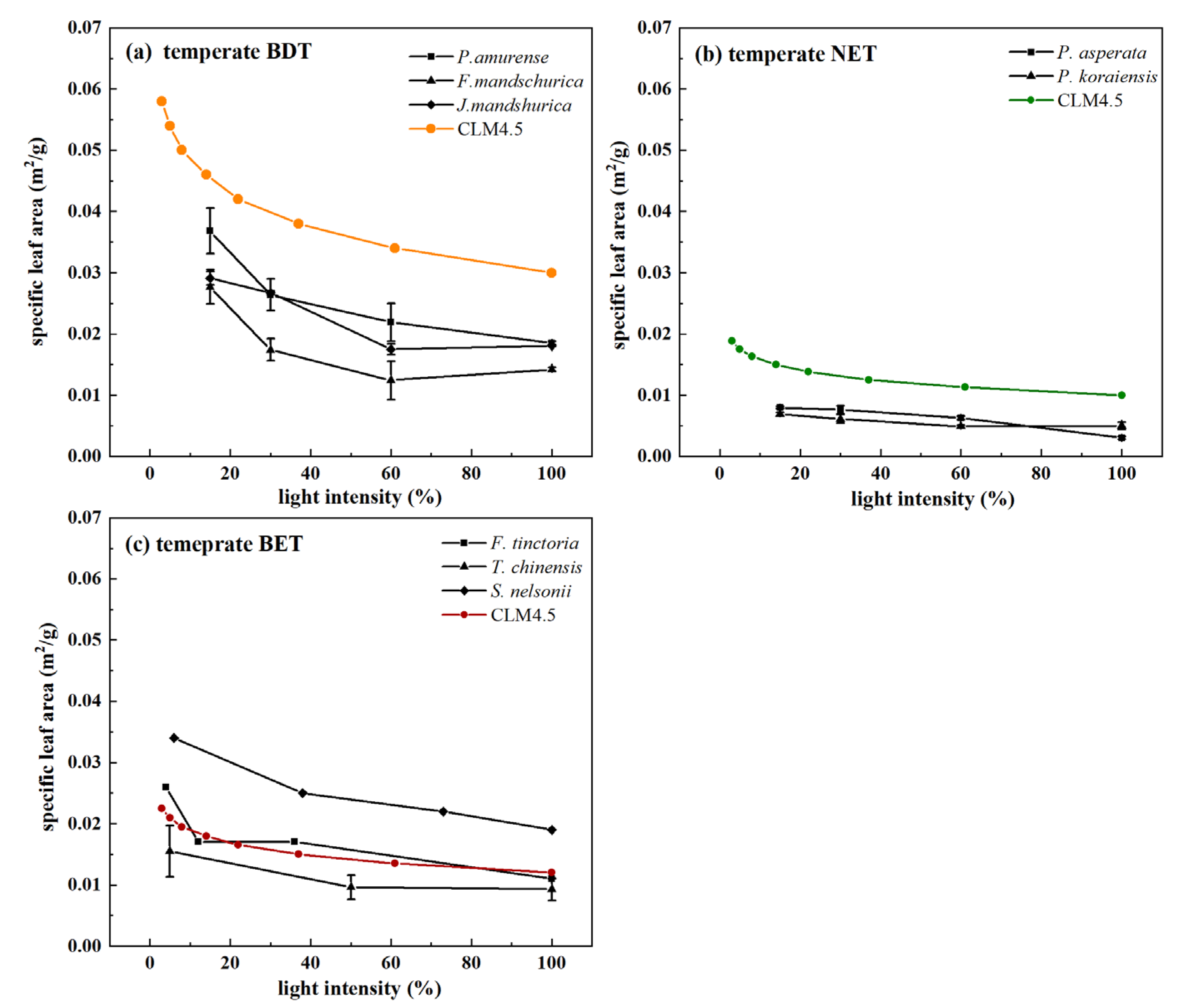
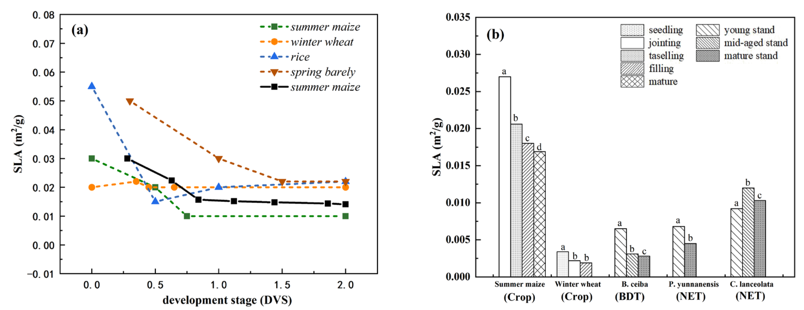
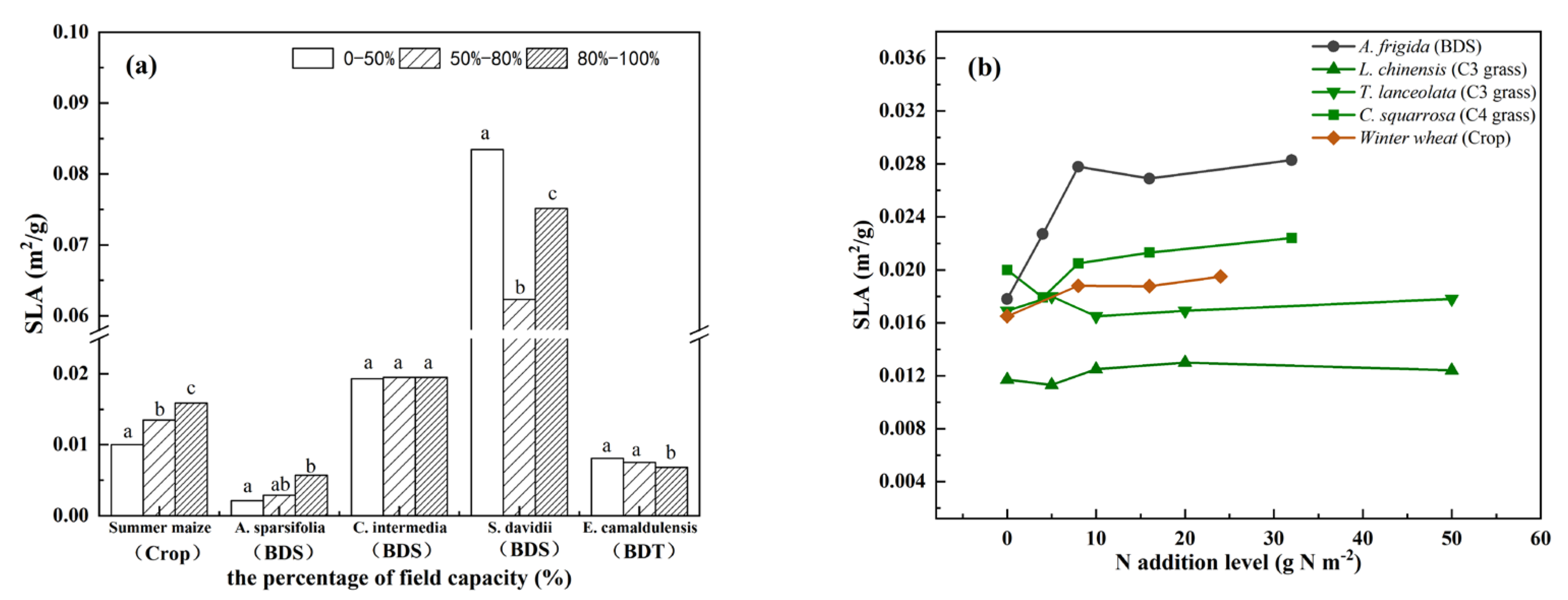
3.2. Interspecific Variation in Observed Plant SLA within Plant Functional Types

The SLA among different species within a given plant functional type in China showed large variability. The observed plant SLA varied from 0.0002 m2/g to 0.0997 m2/g, with a mean variation coefficient (CV) of 42% across different PFTs (Table 2). The interspecific variations in SLA were relatively small for tropical BET, boreal BDT, and boreal BDS, with the CV values varying from 21% to 29%, but were large for the remaining PFTs, with the CV values ranging from 40% to 59%. Among the different tree and shrub types, temperate BDT and temperate BDS had the largest CV of SLA, respectively. Moreover, temperate plants with a great interspecific diversity showed higher SLA variability than tropical and boreal plants in China. Specifically, the CV of SLA for temperate BDT was two times that for boreal BDT.

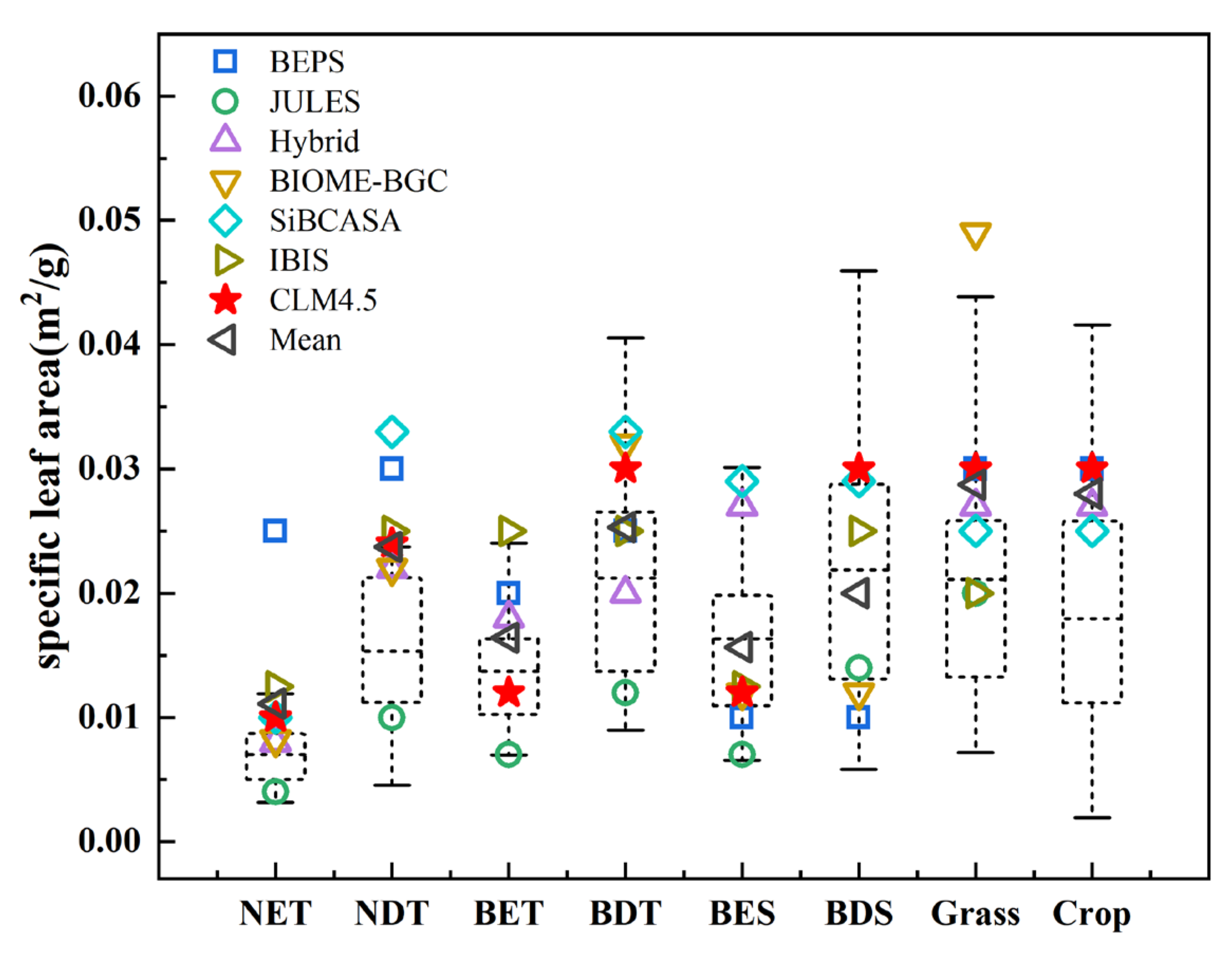
3.3. Variation in the Parameter Values of SLA among Different Terrestrial Biosphere Models

Figure 4 displayed the variation in default SLA values among seven terrestrial biosphere models within eight plant functional types, compared with the observed SLA data. Almost all default SLA value settings in the models for each PFT were in the range of the observed SLA values in China but had large differences within the same PFT. The CV of the default SLA values across models within one PFT varied from 8.7% for crop to 60.0% for NET. Particularly, the SLA value of grass in the BIOME-BGC model was higher than that in the other models by 0.024 m2/g on average, although SLA variation in grass across the seven models was relatively low. The SLA values for the PFTs of BES and NDT in the SiBCASA model were high, which were greater than that of the others by 0.016 m2/g and 0.011 m2/g, respectively. By contrast, the SLA values in the JULES model were generally lower than that in the other models by 0.011 m2/g on average for all PFTs. The variation in SLA value assigned among models for a given PFT was lower than that from the observations, except for NET, BET, and BES. Specifically, the CV of SLA values among models for NET was higher than the CV of observed values by 17.1%.
The mean default values across models for a given PFT was greater than the observed mean by 0.004 m2/g on average (Figure 4). The difference was largest for crop, reaching 0.009 m2/g, followed by NDT, with 0.0087 m2/g. The mean default SLA values across different models were approximately equal with the observed mean for BES. In addition, the default SLA values in few models were close to the mean observed values. For example, the SLA value of BET in the CLM4.5 model was 0.012 m2/g and the average observation was 0.014 m2/g. The difference in SLA values between the hybrid model and the observed mean was only 0.001 m2/g.

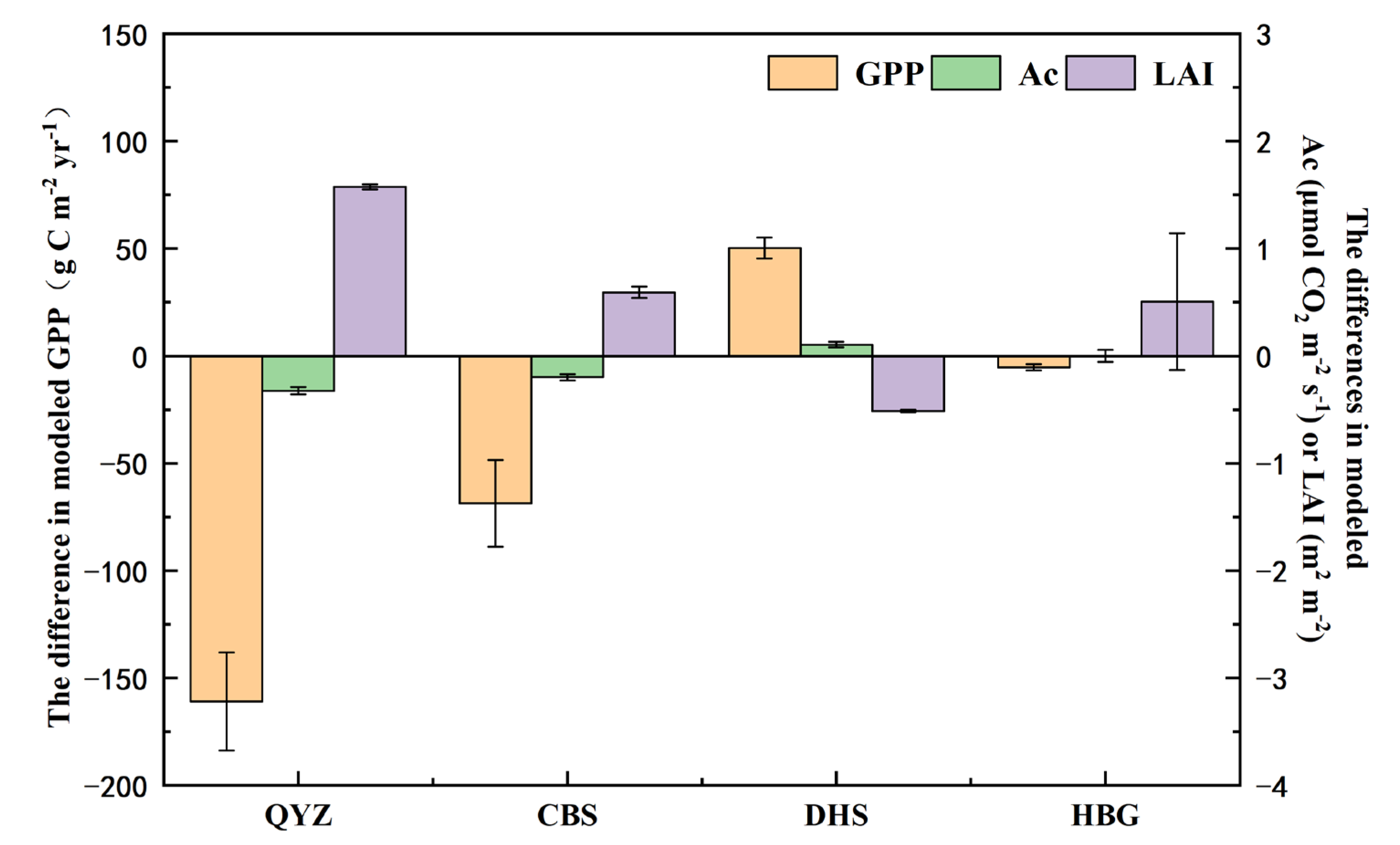
3.4. Impacts of Variation in SLA on Modeled Gross Primary Productivity

We first estimated the differences in CLM4.5-modeled gross primary productivity (GPP) at the QYZ, CBS, DHS, and HBG sites between model experiment S2 using the observed SLA values and model experiment S1 with the default SLA values. Figure 5 presented the changes in annual GPP, mean photosynthesis rate (Ac), and mean leaf area index (LAI) at four sites in the experiment S1 compared with those in experiments S2. The mismatch in SLA between default values in CLM4.5 and observations had a larger influence on GPP simulation for temperate NET (QYZ) and temperate BET (CBS) than that for temperate BDT (DHS) and grass (HBG). The overestimation of the default SLA value by 0.003 m2/g for temperate NET could result in a lower annual GPP estimation at QYZ by 161 g C m−2 yr−1. This weakened productivity was mainly caused by a decrease in the photosynthesis rate in spite of an increase in LAI. Similarly, the higher default SLA value for temperate BDT by 0.008 m2/g, induced a lower modeled GPP at CBS by 69 g C m−2 yr−1. On the contrary, a 0.002 m2/g underestimation of the SLA value for temperate BET in the CLM4.5 caused a decrease in LAI and a slight increase in Ac, which led to a higher annual GPP by 51 g C m−2 yr−1. In addition, a large, overvalued SLA in CLM4.5 for C3 grass had a small impact of 5 g C m−2 yr−1 on simulated GPP and Ac at HBG, although there was an increase in LAI by 0.3 m2/m2.
We then quantified the impacts of SLA variation calculated from the observations and models on the modeled GPP at these sites. Table 3 presents the CV of SLA quantified by observed data (Table 2) and default values across seven terrestrial biosphere models (Figure 4), and the corresponding relative changes in modeled GPP, Ac, and LAI with the involvement of these variation in SLA calculated by Equations (7) and (8), respectively. The results showed a larger influence on modeled GPP at QYZ and DHS than that at the CBS and HBG sites due to the variation of the SLA values. The SLA values in temperate NET and temperate BET both changed by 43% at the mean observed level, which caused the modeled GPP at QYZ and DHS to change by 7% and 8%, respectively. The observed SLA variations in temperate BDT and C3 grass had little impact on the GPP simulation at CBT and HBG, although Ac and LAI changed greatly. In particular, the SLA value of C3 grass changed by 57% at the mean observed level and could lead to Ac and LAI changes by 48% and 58%, while GPP at the HBG site only changed by 3%. Moreover, a large SLA variation among models in temperate NET and temperate BET could result in greater impacts on the modeled GPP than the effects from variations in the observation. For example, SLA variation among the models with a CV of 60% in temperate NET caused a GPP change of 19%, resulting from changes in Ac with 31% and LAI with 62% at QYZ.

4. Discussion

Although current terrestrial biosphere models generally consider the differences in SLA among plant functional types (PFTs), there still remain mismatches in SLA values between model and observations. Our results suggested a remarkable mismatch of SLA between the CLM4.5 model and observations collected in China, especially for tropical broadleaf deciduous tree overestimated by 0.013 m2/g (Figure 2). It is necessary for us to revise the SLA values when we use the CLM4.5 model to simulate terrestrial carbon cycle dynamics at the regional scale. Our results also showed that the observed SLA values for China plant were higher than the global average for all PFTs (Figure 6), which is supported by a recent work showing that SLA in Asia was higher than that in Europe and North America by about 0.004 m2/g and 0.001 m2/g for a given leaf dry matter content of 0.25 g/g [44]. The higher values of SLA in Asia and China might be caused by intense resource competition stress, where the communities are dominated by more acquisitive species with high SLA [45]. Therefore, simply referring to other models or global traits data to set SLA values in a regional gross primary productivity simulation study is unreliable. Furthermore, since the observed SLA data for some plant functional types (e.g., temperate BDT, temperate BET, and C3 grass) in China and around the world do not follow normal distributions [9,46], the default model values and mean observed values remain uncertain. We recommend using the probability density distribution of observed trait data within a given PFT rather than setting trait parameter values based on the mean values.
The SLA among species within a given plant functional type has substantial variability in China and other regions due to differences in the genotype and environmental changes [47,48], especially climate and soil factors, e.g., temperature, light, precipitation, and soil nutrient [49,50]. As trait variation was revealed by previous studies as inducing large effects on the simulations of ecosystem productivity (e.g., GPP, NPP, and NEP) and biomass (e.g., vegetation biomass and litter pool) [21,23,51], our results also suggested that SLA observation variation could bring great uncertainty to the GPP simulation, especially for temperate NET and temperate BET. As shown in Table 3, the SLA value varying by 43% at the mean observation level could induce a change in the simulated annual GPP by 161 g C m2 yr1 (7.0%) for temperate NET. It is necessary to describe trait variation within each plant functional type to reduce model uncertainties.
The responses of plant SLA to environmental changes, as shown in previous studies, have also not been well quantified in terrestrial biosphere models. The SLA vertical variability under the change of light in canopy involved in the CLM4.5 model has not been considered in many other terrestrial biosphere models (Figure 2). Moreover, the variation in SLA with development stages was only simulated in some crop models, such as the WOFOST (World Food Studies) model [52], as shown in Figure 7a. These variations in SLA at different growth stages for both crops and trees (Figure 7b) should be added to terrestrial biosphere models in the future. In addition, SLA also varies with other factors, such as water stress (Figure 8a) and soil nitrogen content (Figure 8b), which need to be paid more attention in terrestrial biosphere models.
Within a given plant functional type, plants grouped by morphology and structure may better describe the variability in traits [66,67]. In the Functionally Assembled Terrestrial Ecosystem Simulator (FATES) in CLM5.0, the plant population in each patch is divided first into plant functional types, and each plant type is presented as numerous height classes, according to tree height, diameter, canopy layer, and other variables [68]. Trait–climate relationships have also been analyzed in few modelling studies. For instance, SLA, Vcmax25, and Jcmax25 within the PFTs were re-parameterized yearly depending on the local climatic conditions (e.g., MAT, MAP, and soil moisture) in the JSBACH model [69]. Yang et al. used trait–climate relationships to predict the spatial patterns of LMA, Nmass, and LAI and then simulated vegetation distributions and vegetation responses to climate changes in China using a Gaussian mixture model trained with these trait data [70]. However, the underlying mechanisms behind these trait–climate relationships require more long-term observations, to be able to simulate vegetation responses to future climate change.
The collected SLA data in this study mainly distributed in temperate and subtropical forest and grassland ecosystems, SLA observations in boreal ecosystems, woody plants in the Tibetan Plateau region, and crops were relatively few, and need to be supplemented by further research. Different protocols for measuring SLA (e.g., all leaves vs. the topmost leaf, with vs. without petioles) have been used in published studies [15], which may cause bias in data statistics and analysis. The methods, time, and positions of sampling should be standardized in the future to enhance the representativeness of the plant trait database, especially at the region scale. This paper only quantified the impacts of SLA variation on GPP simulation with the CLM4.5 model for four PFTs; its effects in other PFTs and terrestrial biosphere models need to be further investigated.

5. Conclusions

In this study, we evaluated the CLM4.5-simulated SLA against the observed data collected from China and examined the impacts of SLA variation on GPP simulation using the CLM4.5 model. The results showed that CLM4.5 overestimated the default SLA values at the top of canopy for 11 PFTs and the canopy gradient of SLA for temperate BDT and temperate NET. The higher default SLA values in temperate NET, temperate BDT, and C3 grass caused an underestimation in the modeled GPP at the QYZ, CBS, and HBG sites compared with the results from the mean SLA observations. Substantial SLA variation could cause great changes in modeled GPP, especially for temperate NET and temperate BET. Our study suggested that the interspecific variation in SLA within a given PFT and its responses to environmental changes should be considered in terrestrial biosphere models to reduce the uncertainties in GPP and LAI estimations. More efforts are needed to make full use of the plant trait database to understand the underlying mechanisms of trait variation and to promote model development so as to enhance the prediction ability of ecosystem responses to future climate changes.

Supplementary Materials

The following supporting information can be downloaded at: https://www.mdpi.com/article/10.3390/f14010164/s1, Table S1: The SLA values for different plant functional types between the CLM4.5 model and the observation data in China; Table S2: Plant SLA information in multiple environmental factor experiments.

Author Contributions

Conceptualization, L.Z. and Y.Z.; Methodology, Y.Z. and L.Z.; Software, Y.Z., P.L. and Y.L.; Validation, P.L. and Y.Z.; Formal Analysis, Y.Z., L.Z. and X.R.; Resources, Y.Z., P.L., H.H. and Y.M.; Writing—Original Draft Preparation, Y.Z.; Writing—Review and Editing, L.Z., X.R. and H.H.; Funding Acquisition, L.Z. and H.H. All authors have read and agreed to the published version of the manuscript.

Funding

This work was funded by the National Natural Science Foundation of China (31971512, 42030509, 42141005, 31988102).

Data Availability Statement

The China plant SLA dataset supporting the results is publicly available. This dataset can be found here: https://www.scidb.cn/s/IBvUZj (accessed on 6 August 2022).

Acknowledgments

We thank all related staff of Qianyanzhou site, Changbaishan site, Dinghushan site, and Haibei site from ChinaFLUX and CERN for their contributions, from observations to data processing.

Conflicts of Interest

The authors declare no conflict of interest.

References

  1. Violle, C.; Navas, M.L.; Vile, D.; Kazakou, E.; Fortunel, C.; Hummel, I.; Garnier, E. Let the concept of trait be functional! Oikos 2007, 116, 882–892. [Google Scholar] [CrossRef]
  2. Lavorel, S.; Garnier, E. Predicting changes in community composition and ecosystem functioning from plant traits: Revisiting the Holy Grail. Funct. Ecol. 2002, 16, 545–556. [Google Scholar] [CrossRef]
  3. Wright, I.J.; Reich, P.B.; Cornelissen, J.H.C.; Falster, D.S.; Groom, P.K.; Hikosaka, K.; Lee, W.; Lusk, C.H.; Niinemets, U.; Oleksyn, J.; et al. Modulation of leaf economic traits and trait relationships by climate. Glob. Ecol. Biogeogr. 2005, 14, 411–421. [Google Scholar] [CrossRef]
  4. Osnas, J.L.D.; Lichstein, J.W.; Reich, P.B.; Pacala, S.W. Global Leaf Trait Relationships: Mass, Area, and the Leaf Economics Spectrum. Science 2013, 340, 741–744. [Google Scholar] [CrossRef] [PubMed]
  5. Reich, P.B. The world-wide ‘fast-slow’ plant economics spectrum: A traits manifesto. J. Ecol. 2014, 102, 275–301. [Google Scholar] [CrossRef]
  6. Westoby, M.; Wright, I.J. Land-plant ecology on the basis of functional traits. Trends Ecol. Evol. 2006, 21, 261–268. [Google Scholar] [CrossRef] [PubMed]
  7. Finegan, B.; Peña-Claros, M.; Oliveira, A.; Ascarrunz, N.; Bret-Harte, M.S.; Carreño-Rocabado, G.; Casanoves, F.; Díaz, S.; Velepucha, P.E.; Fernandez, F.; et al. Does functional trait diversity predict above-ground biomass and productivity of tropical forests? Testing three alternative hypotheses. J. Ecol. 2015, 103, 191–201. [Google Scholar] [CrossRef] [Green Version]
  8. Reich, P.B.; Ellsworth, D.S.; Walters, M.B.; Vose, J.M.; Gresham, C.; Volin, J.C.; Bowman, W.D. Generality of leaf trait relationship: A test across six biomes. Ecology 1999, 80, 1955–1969. [Google Scholar] [CrossRef]
  9. Kattge, J.; DÍAz, S.; Lavorel, S.; Prentice, I.C.; Leadley, P.; BÖNisch, G.; Garnier, E.; Westoby, M.; Reich, P.B.; Wright, I.J.; et al. TRY- a global database of plant traits. Glob. Change Biol. 2011, 17, 2905–2935. [Google Scholar] [CrossRef]
  10. Wang, R.L.; Yu, G.R.; He, N.P.; Wang, Q.F.; Zhao, N.; Xu, Z.W. Latitudinal variation of leaf morphological traits from species to communities along a forest transect in eastern China. J. Geogr. Sci. 2016, 26, 15–26. [Google Scholar] [CrossRef]
  11. Wang, H.; Prentice, I.C.; Ni, J. Data-based modelling and environmental sensitivity of vegetation in China. Biogeosciences 2013, 10, 5817–5830. [Google Scholar] [CrossRef] [Green Version]
  12. Liu, Z.G.; Zhao, M.; Zhang, H.X.; Ren, T.T.; Liu, C.C.; He, N.P. Divergent response and adaptation of specific leaf area to environmental change at different spatial-temporal scales jointly improve plant survival. Glob. Change Biol. 2022, in press. [Google Scholar] [CrossRef] [PubMed]
  13. Reich, P.B.; Ellsworth, D.S.; Walters, M.B. Leaf structure (specific leaf area) modulates photosynthesis–nitrogen relations: Evidence from within and across species and functional groups. Funct. Ecol. 1998, 12, 948–958. [Google Scholar] [CrossRef]
  14. Lavorel, S.; Díaz, S.; Cornelissen, J.H.C.; Garnier, E.; Harrison, S.P.; Mclntyre, S.; Pausas, J.G.; Pérez-Harguindeguy, N.; Roumet, C.; Urcelay, C. Plant functional types: Are we getting any closer to the holy grail. In Terrestrial Ecosystems in a Changing World; Canadell, J.G., Pataki, D.E., Pitelka, L.F., Eds.; Springer: Berlin/Heidelberg, Germany, 2007; pp. 149–164. [Google Scholar]
  15. Yang, Y.Z.; Wang, H.; Zhu, Q.; Wen, Z.M.; Peng, C.H.; Lin, G.H. Research progresses in improving dynamic global vegetation models (DGVMs) with plant functional traits. Chin. Sci. Bull. 2018, 63, 2599–2611. [Google Scholar] [CrossRef] [Green Version]
  16. Raulier, F.; Bernier, P.Y.; Ung, C.-H. Canopy photo-synthesis of sugar maple (Acer saccharum): Comparing big-leaf and multilayer extrapolations of leaf-level measure-ments. Tree Physiol. 1999, 19, 407–442. [Google Scholar] [CrossRef] [Green Version]
  17. Thornton, P.E.; Zimmermann, N.E. An improved canopy integration scheme for a land surface model with prognostic canopy structure. J. Clim. 2007, 20, 3902–3923. [Google Scholar] [CrossRef]
  18. Harper, A.B.; Cox, P.M.; Friedlingstein, P.; Wiltshire, A.J.; Jones, C.D.; Sitch, S.; Mercado, L.M.; Groenendijk, M.; Robertson, E.; Kattge, J.; et al. Improved representation of plant functional types and physiology in the Joint UK Land Environment Simulator (JULES v4.2) using plant trait information. Geosci. Model Dev. 2016, 9, 2415–2440. [Google Scholar] [CrossRef] [Green Version]
  19. Wramneby, A.; Smith, B.; Zaehle, S.; Sykes, M.T. Parameter uncertainties in the modeling of vegetation dynamics-effects on tree community structure and ecosystem functioning in European forest biomes. Ecol. Modell. 2008, 216, 277–290. [Google Scholar] [CrossRef]
  20. Cui, E.Q.; Huang, K.; Arain, M.A.; Fisher, J.B.; Huntzinger, D.N.; Ito, A.; Luo, Y.Q.; Jain, A.K.; Mao, J.F.; Michalak, A.M.; et al. Vegetation Functional Properties Determine Uncertainty of Simulated Ecosystem Productivity: A Traceability Analysis in the East Asian Monsoon Region. Glob. Biogeochem. Cycles 2019, 33, 668–689. [Google Scholar] [CrossRef] [Green Version]
  21. Zhang, H.C.; Liu, D.; Dong, W.J.; Cai, W.W.; Yuan, W.P. Accurate representation of leaf longevity is important for simulating ecosystem carbon cycle. Basic Appl. Ecol. 2016, 17, 396–407. [Google Scholar] [CrossRef]
  22. Feng, X.; Liu, G.; Chen, J.M.; Chen, M.; Liu, J.; Ju, W.M.; Sun, R.; Zhou, W. Net primary productivity of China’s terrestrial ecosystems from a process model driven by remote sensing. J. Environ. Manag. 2007, 85, 563–573. [Google Scholar] [CrossRef]
  23. White, M.A.; Thornton, P.E.; Running, S.W.; Nemani, R.R. Parameterization and sensitivity analysis of the BIOME-BGC terrestrial ecosystem model: Net primary production controls. Earth Interact. 2000, 4, 1–85. [Google Scholar] [CrossRef]
  24. Schaefer, K.; Collatz, G.J.; Tans, P.; Denning, A.S.; Baker, I.; Berry, J.; Prihodko, L. Combined Simple Biosphere/Carnegie-Ames-Stanford Approach terrestrial carbon cycle model. J. Geophys. Res. Biogeosci. 2006, 113, 603. [Google Scholar] [CrossRef]
  25. Oleson, K.W.; Lawrence, D.M.; Bonan, G.B.; Drewniak, B.; Huang, M.Y.; Koven, C.D.; Levis, S.; Li, F.; Riley, W.J.; Subin, Z.M.; et al. Technical Description of Version 4.5 of the Community Land Model (CLM); Ncar Technical Note NCAR/TN-503 + STR; National Center for Atmospheric Research: Boulder, CO, USA, 2013. [Google Scholar]
  26. Kucharik, C.J.; Foley, J.A.; Delire, C.; Fisher, V.A.; Coe, M.T.; Lenters, J.D.; Young-Molling, C.; Ramankutty, N.; Norman, J.M.; Gower, S.T. Testing the performance of a dynamic global ecosystem model: Water balance, carbon balance, and vegetation structure. Glob. Biogeochem. Cycles 2000, 14, 795–825. [Google Scholar] [CrossRef]
  27. Zhang, L.; Mao, J.F.; Shi, X.Y.; Ricciuto, D.; He, H.L.; Thornton, P.; Yu, G.R.; Li, P.; Liu, M.; Ren, X.L.; et al. Evaluation of the Community Land Model simulated carbon and water fluxes against observations over ChinaFLUX sites. Agric. For. Meteorol. 2016, 226, 174–185. [Google Scholar] [CrossRef] [Green Version]
  28. Fox, A.M.; Hoar, T.J.; Anderson, J.L.; Arellano, A.F.; Smith, W.K.; Litvak, M.E.; MacBean, N.; Schimel, D.S.; Moore, D.J.P. Evaluation of a Data Assimilation System for Land Surface Models Using CLM4.5. J. Adv. Model. Earth Syst. 2018, 10, 2471–2494. [Google Scholar] [CrossRef]
  29. Post, H.; Vrugt, J.A.; Fox, A.; Vereecken, H.; Franssen, H.-J.H. Estimation of Community Land Model parameters for an improved assessment of net carbon fluxes at European sites. Biogeosciences 2017, 122, 661–689. [Google Scholar] [CrossRef] [Green Version]
  30. Mao, J.F.; Fu, W.T.; Shi, X.Y.; Ricciuto, D.M.; Fisher, J.B.; Dickinson, R.E.; Wei, Y.X.; Shem, W.; Piao, S.L.; Wang, K.C. Disentangling climatic and anthropogenic controls on global terrestrial evapotranspiration trends. Environ. Res. Lett. 2015, 10, 094008. [Google Scholar] [CrossRef]
  31. Shi, X.Y.; Mao, J.F.; Thornton, P.E.; Huang, M.Y. Spatiotemporal patterns of evapotranspiration in response to multiple environmental factors simulated by the community land model. Environ. Res. Lett. 2013, 8, 024012. [Google Scholar] [CrossRef]
  32. Lawrence, P.J.; Chase, T.N. Representing a new MODIS consistent land surface in the community land model (CLM 3.0). J. Geophys. Res. Biogeosci. 2007, 112, G01023. [Google Scholar] [CrossRef]
  33. Scanlon, B.R.; Zhang, Z.; Save, H.; Sun, A.Y.; Schmied, H.M.; van Beek, L.P.H.; Wiese, D.N.; Wada, Y.; Long, D.; Reedy, R.C.; et al. Global models underestimate large decadal declining and rising water storage trends relative to GRACE satellite data. Proc. Natl. Acad. Sci. USA 2018, 115, E1080–E1089. [Google Scholar] [CrossRef] [PubMed] [Green Version]
  34. Li, C.W.; Lu, H.; Yang, K.; Han, M.L.; Wright, J.S.; Chen, Y.Y.; Yu, L.; Xu, S.M.; Huang, X.M.; Gong, W. The Evaluation of SMAP Enhanced Soil Moisture Products Using High-Resolution Model Simulations and In-Situ Observations on the Tibetan Plateau. Remote sens. 2018, 10, 535. [Google Scholar] [CrossRef] [Green Version]
  35. Farquhar, G.D.; von Caemmerer, S.; Berry, J.A. A biochemical model of photosynthetic CO2 assimilation in leaves of C3 species. Planta 1980, 149, 78–90. [Google Scholar] [CrossRef] [PubMed] [Green Version]
  36. Collatz, G.J.; Ribas-Carbo, M.; Berry, J.A. Coupled photosynthesis-stomatal conductance model for leaves of C4 plants. Aust. J. Plant Physiol. 1992, 19, 519–538. [Google Scholar] [CrossRef]
  37. Thornton, P.E.; Lamarque, J.-F.; Rosenbloom, N.A.; Mahowald, N.M. Influence of carbon-nitrogen cycle coupling on land model response to CO2 fertilization and climate variability. Glob. Biogeochem. Cycles 2007, 21, B002868. [Google Scholar] [CrossRef]
  38. Ali, A.A.; Xu, C.; Rogers, A.; Fisher, R.A.; Wullschleger, S.D.; Massoud, E.; Vrugt, J.A.; Muss, J.D.; McDowell, N.; Fisher, J. A global scale mechanistic model of photosynthetic capacity (LUNA V1. 0). Geosci. Mod. Dev. 2016, 9, 587–606. [Google Scholar] [CrossRef] [Green Version]
  39. Lawrence, D.M.; Fisher, R.A.; Koven, C.D.; Oleson, K.W.; Swenson, S.C.; Bonan, G.; Collier, N.; Ghimire, B.; van Kampenhout, L.; Kennedy, D.; et al. The Community Land Model version 5: Description of new features, benchmarking, and impact of forcing uncertainty. J. Adv. Model. Earth Syst. 2019, 11, 4245–4287. [Google Scholar] [CrossRef] [Green Version]
  40. Li, M.C.; Shu, J.J.; Sun, Y.R. Responses of specific leaf area of dominant tree species in Northeast China secondary forests to light intensity. Chin. J. Ecol. 2009, 28, 1437–1442. [Google Scholar] [CrossRef]
  41. Zhang, Y.J.; Feng, Y.L. Relationship between leaf photosynthetic capacity and specific leaf weight, nitrogen content and allocation of two ficus species under different light intensities. J. Plant Physiol. Mol. Biol. 2004, 30, 269–276. [Google Scholar]
  42. Liu, W.D.; Li, S.F.; Su, L.; Su, J. Variation and correlations of leaf traits of two Taxus species with different shade tolerance along the light gradient. Pol. J. Ecol. 2013, 61, 329–339. [Google Scholar]
  43. Deloso, B.E.; Marler, T.E. Bi-Pinnate compound Serianthes nelsonii leaf-level plasticity magnifies leaflet-level plasticity. Biology 2020, 9, 333. [Google Scholar] [CrossRef] [PubMed]
  44. Ren, L.; Huang, Y.M.; Pan, Y.P.; Xiang, X.; Huo, J.X.; Meng, D.H.; Wang, Y.Y.; Yun, C. Differential Investment Strategies in Leaf Economic Traits Across Climate Regions Worldwide. Front. Plant Sci. 2022, 13, 798035. [Google Scholar] [CrossRef]
  45. Heberling, J.M.; Fridley, J.D. Biogeographic constraints on the world-wide leaf economics spectrum. Glob. Ecol. Biogeogr. 2012, 21, 1137–1146. [Google Scholar] [CrossRef]
  46. Liu, K.J.; He, N.P.; Hou, J.H. Spatial patterns and influencing factors of specific leaf area in typical temperate forests. Acta Ecol. Sin. 2022, 42, 872–883. [Google Scholar] [CrossRef]
  47. Auger, S.; Shipley, B. Inter-specific and intra-specific trait variation along short environmental gradients in an old-growth temperate forest. J. Veg. Sci. 2013, 24, 419–428. [Google Scholar] [CrossRef]
  48. Mudrak, O.; Dolezal, J.; Vitova, A.; Leps, J. Variation in plant functional traits is best explained by the species identity: Stability of trait-based species ranking across meadow management regimes. Funct. Ecol. 2019, 33, 746–755. [Google Scholar] [CrossRef]
  49. Poorter, H.; Niinemets, U.; Poorter, L.; Wright, I.J.; Villar, R. Causes and consequences of variation in leaf mass per area (LMA): A meta-analysis. New Phytol. 2009, 182, 565–588. [Google Scholar] [CrossRef]
  50. Yang, Y.Z.; Gou, R.K.; Li, W.; Kassout, J.; Wu, J.; Wang, L.M.; Peng, C.H.; Lin, G.H. Leaf Trait Covariation and Its Controls: A Quantitative Data Analysis Along a Subtropical Elevation Gradient. J. Geophys. Res. Biogeosci. 2021, 126, e2021JG006378. [Google Scholar] [CrossRef]
  51. Koven, C.D.; Knox, R.G.; Fisher, R.A.; Chambers, J.Q.; Christoffersen, B.O.; Davies, S.J.; Detto, M.; Dietze, M.C.; Faybishenko, B.; Holm, J.; et al. Benchmarking and parameter sensitivity of physiological and vegetation dynamics using the Functionally Assembled Terrestrial Ecosystem Simulator (FATES) at Barro Colorado Island, Panama. Biogeosciences 2020, 17, 3017–3044. [Google Scholar] [CrossRef]
  52. De Wit, A.; Boogaard, H.; Fumagalli, D.; Janssen, S.; Knapen, R.; van Kraalingen, D.; Supit, I.; van der Raymond, W.; van Diepen, K. 25 years of the WOFOST cropping systems model. Agric. Syst. 2019, 168, 154–167. [Google Scholar] [CrossRef]
  53. Wu, R.; Yan, X.H.; Li, Y.N. Effects of Film Mulching and Supplementary Irrigation on Chlorophyll and Specific Leaf Area of Winter Wheat. Water Sav. Irrig. 2018, 9, 27–36. [Google Scholar]
  54. Cao, Y.H.; Shi, J.G.; Zhu, K.L.; Dong, S.T.; Liu, P.; Zhao, B.; Zhan, gJ.W. Effects of sowing depth on canopy structure and photosynthetic characteristics of summer maize. J. Maize. Sci. 2016, 24, 102–109. [Google Scholar] [CrossRef]
  55. Yang, Q.; Zhu, R.J.; Yang, C.Y.; Li, S.J.; Cheng, X.P. Variation in leaf functional traits of Bombax ceiba Linnaeus communities based on tree structure. Acta Ecol. Sin. 2022, 42, 2834–2842. [Google Scholar] [CrossRef]
  56. Zhang, L.; Luo, T.X.; Deng, K.M.; Li, W.H. Vertical variations in specific leaf area and leaf dry matter content with canopy height in Pinus yunnanensis. J. Beijing For. Univ. 2008, 30, 40–44. [Google Scholar] [CrossRef]
  57. Peng, X.; Yan, W.D.; Wang, F.Q.; Wang, G.J.; Yu, F.Y.; Zhao, M.F. Specific leaf area estimation model building based on leaf dry matter content of Cunninghamia lanceolata. Chin. J. Plant Ecol. 2018, 42, 209–219. [Google Scholar] [CrossRef] [Green Version]
  58. Rad, M.H.; Assare, M.H.; Banakar, M.H.; Soltani, M. Effects of Different Soil Moisture Regimes on Leaf Area Index, Specific Leaf Area and Water use Efficiency in Eucalyptus (Eucalyptus camaldulensis Dehnh) under Dry Climatic Conditions. Asian J. Plant Sci. 2011, 10, 294–300. [Google Scholar] [CrossRef] [Green Version]
  59. Zhang, C.Z.; Zhang, J.B.; Zhang, H.; Zhao, J.H.; Wu, Q.C.; Zhao, Z.H.; Cai, T.Y. Mechanisms for the relationships between water-use efficiency and carbon isotope composition and specific leaf area of maize (Zea mays L.) under water stress. Plant Growth Regul. 2015, 77, 233–243. [Google Scholar] [CrossRef]
  60. Huang, C.B.; Zeng, F.J.; Lei, J.Q. Growth and functional trait responses of Alhagi sparsifolia seedlings to water and nitrogen addition. Acta Prataculturae Sin. 2016, 25, 150–160. [Google Scholar] [CrossRef]
  61. Xiao, C.W.; Sun, O.J.; Zhou, G.S.; Zhao, J.Z.; Wu, G. Interactive effects of elevated CO2 and drought stress on leaf water potential and growth in Caragana intermedia. Trees 2005, 19, 712–721. [Google Scholar] [CrossRef]
  62. Wu, F.Z.; Bao, W.K.; Li, F.L.; Wu, N. Effects of water stress and nitrogen supply on leaf gas exchange and fluorescence parameters of Sophora davidii seedlings. Photosynthetica 2008, 46, 40–48. [Google Scholar] [CrossRef]
  63. Huang, J.Y.; Yu, H.L.; Yuan, Z.Y.; Li, L.H. Effects of long-term increased soil N on leaf traits of several species in typical Inner Mongolian grassland. Acta Ecol. Sin. 2009, 32, 1419–1427. [Google Scholar] [CrossRef] [Green Version]
  64. Sun, L.; Yang, G.; Zhang, Y.; Qin, S.; Dong, J.; Cui, Y.; Liu, X.; Zheng, P.; Wang, R. Leaf Functional Traits of Two Species Affected by Nitrogen Addition Rate and Period Not Nitrogen Compound Type in a Meadow Grassland. Front. Plant Sci. 2022, 13, 841464. [Google Scholar] [CrossRef] [PubMed]
  65. Ratjen, A.M.; Kage, H. Is mutual shading a decisive factor for differences in overall canopy specific leaf area of winter wheat crops? Field Crops Res. 2013, 149, 338–346. [Google Scholar] [CrossRef]
  66. Van Bodegom, P.M.; Douma, J.C.; Verheijen, L.M. A fully traits-based approach to modeling global vegetation distribution. Proc. Natl. Acad. Sci. USA 2014, 111, 13733–13738. [Google Scholar] [CrossRef] [Green Version]
  67. Thomas, H.J.D.; Myers-Smith, I.H.; Bjorkman, A.D.; Elmendorf, S.C.; Blok, D.; Cornelissen, J.H.C.; Forbes, B.C.; Hollister, R.D.; Normand, S.; Prevey, J.S.; et al. Traditional plant functional groups explain variation in economic but not size-related traits across the tundra biome. Glob. Ecol. Biogeogr. 2019, 28, 78–95. [Google Scholar] [CrossRef] [Green Version]
  68. Fisher, R.A.; Muszala, S.; Verteinstein, M.; Lawrence, P.; Xu, C.; McDowell, N.G.; Knox, R.G.; Koven, C.; Holm, J.; Rogers, B.M.; et al. Taking off the training wheels: The properties of a dynamic vegetation model without climate envelopes, CLM4.5(ED). Geosci. Model Dev. 2015, 8, 3593–3619. [Google Scholar] [CrossRef] [Green Version]
  69. Verheijen, L.M.; Brovkin, V.; Aerts, R.; Bonisch, G.B.; Cornelissen, J.H.C.; Kattge, J.; Reich, P.B.; Wright, I.J.; van Bodegom, P.M. Impacts of trait variation through observed trait-climate relationships on performance of an Earth system model: A conceptual analysis. Biogeosciences 2013, 10, 5497–5515. [Google Scholar] [CrossRef] [Green Version]
  70. Yang, Y.Z.; Zhu, Q.A.; Peng, C.H.; Wang, H.; Xue, W.; Lin, G.H.; Wen, Z.M.; Chang, J.; Wang, M.; Liu, G.B.; et al. A novel approach for modelling vegetation distributions and analysing vegetation sensitivity through trait-climate relationships in China. Sci. Rep. 2016, 6, 24110. [Google Scholar] [CrossRef] [PubMed]
Figure 1. Distribution of observed specific leaf area (SLA) data in China.
Forests 14 00164 g001
Figure 2. The differences in specific leaf area (SLA) between observation data in China and default values in the CLM4.5 model. The error bar shows the standard deviation. 1, temperate NET; 2, boreal NET; 3, boreal NDT; 4, tropical BET; 5, temperate BET; 6, tropical BDT; 7, temperate BDT; 8, boreal BDT; 9, temperate BES; 10, temperate BDS; 11, boreal BDS; 12, C3 grass; 13, C4 grass; 14, rainfed crop.
Forests 14 00164 g002
Figure 3. The responses of specific leaf area (SLA) to light gradients for temperate broadleaf deciduous tree (BDT) (a), temperate needleleaf evergreen tree (NET) (b), and temperate broadleaf evergreen tree (BET) (c). More details about the species can be found in Table S2 [40,41,42,43].
Forests 14 00164 g003
Figure 4. The default SLA values in terrestrial biosphere models and the SLA mean observed values in China for different plant functional types. Box plots show the mean, 25th percentile, and 75th percentile of the observed SLA values. Abbreviations: NET, needleleaf evergreen tree; NDT, needleleaf deciduous tree; BET, broadleaf evergreen tree; BDT, broadleaf deciduous tree; BES, broadleaf evergreen shrub; BDS, broadleaf deciduous shrub.
Forests 14 00164 g004
Figure 5. The differences in annual gross primary productivity (GPP), mean RuBP-limited photosynthesis rate (Ac), mean leaf area index (LAI) between model experiment S1 (with default SLA values in the CLM4.5 model) and model experiment S2 (with mean SLA observed values). The error bar shows the standard deviation. QYZ site: temperate needleleaf evergreen tree; CBS site: temperate broadleaf deciduous tree; DHS site: broadleaf evergreen tree; HBG site: C3 grass.
Forests 14 00164 g005
Figure 6. The differences in SLA values between the observation data in China and the global average in the TRY database. The error bar shows the standard deviation. Abbreviations: NET, needleleaf evergreen tree; NDT, needleleaf deciduous tree; BET, broadleaf evergreen tree; BDT, broadleaf deciduous tree; BES, broadleaf evergreen shrub; BDS, broadleaf deciduous shrub.
Forests 14 00164 g006
Figure 7. The changes in SLA values during key development stages (DVS) for different crops (a) and observed SLA values in various growth periods (b). For (a), the dotted lines are the default SLA values at different DVS in the WOFOST model and the solid line is the observed SLA values of summer maize at the Gucheng site in China. DVS values range from −0.1 at sowing to 0.0 at emergence, 1.0 at flowering, and 2.0 at physiological maturity. For (b), the different lowercase letters indicate significant differences at the 0.05 level. More details about the species can be found in Table S2 [53,54,55,56,57].
Forests 14 00164 g007
Figure 8. The SLA values of different PFTs under three soil moisture regimes (a) and different N addition levels (b). The different lowercase letters indicate significant differences at 0.05 level. More details about the species can be found in Table S2 [58,59,60,61,62,63,64,65].
Forests 14 00164 g008
Table 1. Site information of four ChinaFLUX sites.
Site NameQYZCBSDHSHBG
latitude (E)26.7442.4023.1737.67
longitude (N)115.06128.10112.57101.33
elevation (m)1027383003327
plant functional typetemperate NETtemperate BDTtemperate BETC3 grass
simulated years2003–20082003–20082003–20082003–2008
Table 2. The variation in specific leaf area (SLA) observations among different plant functional types (PFTs) in China. Abbreviations: NET, needleleaf evergreen tree; NDT, needleleaf deciduous tree; BET, broadleaf evergreen tree; BDT, broadleaf deciduous tree; BES, broadleaf evergreen shrub; BDS, broadleaf deciduous shrub.
PFTMaximum SLA Value (m2/g)Minimum SLA Value (m2/g)Coefficient of Variation (%)Number of Samples (n)
temperate NET0.0020.01642.8669
boreal NET0.0030.00840.010
boreal NDT0.0050.02440.011
tropical BET0.0040.02728.57103
temperate BET0.00020.03742.86277
tropical BDT0.0070.03241.189
temperate BDT0.0020.08150.0501
boreal BDT0.0050.02825.04
temperate BES0.0040.04847.06221
temperate BDS0.0020.01059.09454
boreal BDS0.0040.02521.056
C3 grass0.0020.08257.14822
C4 grass0.0030.05247.37126
rainfed crop0.0020.04252.6319
Table 3. The relative changes in GPP, Ac, and LAI modeled with different SLA values. R1 is the relative changes in modeled GPP, Ac, and LAI caused by the observed SLA variation based on model experiments S2, S3, and S4 (Equation (7)). R2 is the relative changes in modeled GPP, Ac, and LAI caused by the SLA variation across models based on model experiments S1, S5, and S6 (Equation (8)). Abbreviations: PFT, plant functional type; NET, needleleaf evergreen tree; BDT, broadleaf deciduous tree; BET, broadleaf evergreen tree.
SitePFTRelative ChangeCV of SLA (%)GPP (%)Ac (%)LAI (%)
QYZtemperate NETR142.97.043.914.1
R260.018.531.061.7
CBStemperate BDTR150.06.330.916.9
R229.48.824.543.8
DHStemperate BETR142.98.037.314.7
R242.814.124.663.7
HBGC3 grassR157.13.357.948.4
R234.31.63.346.2
Disclaimer/Publisher’s Note: The statements, opinions and data contained in all publications are solely those of the individual author(s) and contributor(s) and not of MDPI and/or the editor(s). MDPI and/or the editor(s) disclaim responsibility for any injury to people or property resulting from any ideas, methods, instructions or products referred to in the content.

