1. Introduction
Forest harvesting plays an important role in supplying the economy with a renewable raw material–wood. Global harvesting of industrial roundwood equals 1.98 billion m
3, while in Europe it was 633 million m
3 and, in Poland, 35.8 million m
3 in the year 2020 [
1]. Most of this volume in Europe is procured using modern machinery—harvesters and forwarders—in a cut-to-length system (CTL). Harvesters fell and process the tree, while measuring its characteristics, such as length and diameter, in order to optimize crosscutting into different assortments. From the very beginning of development of these machines, this task required a measuring system, that was quickly computerized [
2]. At present, harvesters benefit from very powerful computer systems that also play an important role in controlling the machine as a whole. Gradually, these systems incorporated the networking functions that allow to monitor and control the whole fleet of machines—even from remote locations. For this reason, it was advisable to equip forwarders with similar systems as well. This is in line with a global trend of implementing the concept of Industry 4.0 (the Fourth Industrial Revolution) that requires an advanced system of information input from the physical environment (machines and their sensors). Such data are later transformed in an external virtual location and enables to actively monitor the performance of machines for the superior goal of optimization of the entire system. In this scenario, a forest machine that is monitored by a multitude of sensors and is connected to a cloud by the Global System for Mobile Communication (GSM) modem, becomes a cybernetic physical unit (CPU) and a part of Internet-of-Things [
3,
4].
A side product of constant data collection from many sensors is an extensive database that is populated automatically, in real-time and without any interaction with the operator. This database is usually accessible by the machine owner or manager, and by the technical support team of the machine supplier. The vast amount of the data makes it sometimes challenging to interpret, especially since not all variables are necessary for every goal, e.g., data concerning the engine performance or machine diagnostics are of limited interest to the harvesting team manager, whereas harvesting volumes and working times are crucial to him, but not necessary to a support technician. Collecting, pre-processing and storing of this data is conducted by a comprehensive computer system usually maintained by the machine’s manufacturer. A list of variables recorded and made available for a harvester is presented in
Supplementary Materials Table S1.
Another potential application for such accurate data is scientific research. Attempts to utilize the readings from on-board computers to analyze forest harvesting operations have been made in the past [
5,
6,
7,
8,
9,
10] and it is now becoming one of the most promising methods of data collection in this field. Information contained in these databases can have many benefits over traditionally acquired measurements—these are long-term, objective, non-biased and are taken automatically. This also means that the operator, while being aware of the fact that he is being constantly recorded, becomes used to it and does not modify his working habits as is often the case with standard measurements, leading to the so-called Hawthorne’s effect [
7,
11]. Another advantage of using machines’ in-built sensors for measurements is connected with obtaining information that would be difficult or even impossible to measure in a traditional way. Detailed information on fuel consumption—broken down into several tasks, such as cutting and processing, engine utilization times at a specific load level—is just one example of data that would be virtually impossible to measure in field conditions. Others—e.g., average cycle times, distances traveled, volume and number of processed trees—are possible to measure, but are labor-intensive and time-consuming, and not feasible for a longer study period [
12,
13]. Additionally, it might be difficult to note and measure short and rapidly changing working elements [
7]. Some disadvantages of automatically collected data concern the accuracy of measurements, which sometimes need to be confirmed by a field study [
14,
15]. Missing data—due to malfunctions or lack of input by the operator—are common and are nearly impossible to rectify. Eventually, not all interesting variables are being measured, which might limit the applicability of the data, but at the same time gives an opportunity to use machine learning techniques to infer the lacking information. Apart from predicting the outcome, the data mining techniques allow to find trends and patterns in extensive and complicated data [
9,
16].
Usually, the data mining cycle requires the following steps (that are later repeated, hence the term ‘cycle’): data acquisition, decision on target data (elimination of redundant variables), pre-processing (‘cleaning’ the incomplete records), transforming (some basic calculations—ratios, unit conversion) and finally, looking for patterns. Information from the last step can also be used to affect previous ones in the next cycle.
Advantages of data mining techniques have been appreciated and used in many fields, from medicine, education, finance and logistics to security. The ability to detect anomalies is used in screening and early prediction of diseases [
17,
18,
19]. Performance of students and academics may be assessed applying various methods [
20], which is especially valuable in distant learning [
21]. Possible applications in security are numerous, from physical protection [
22] to cyber-security [
23]. Additionally, in forestry, data mining is becoming increasingly popular [
24,
25]. Some examples include prediction of forest fires [
26,
27], evaluation of occupational accidents [
28], assessment of potential recreational use of forests [
29], forest inventory [
30,
31] and forest utilization [
2,
9,
16,
32,
33].
Most of the published research concerning forestry machine performance, utilizes data from harvesters in the form of StanForD files [
7,
8,
9,
16,
34]. StanForD is a widely accepted system of communication between computers in forestry machines; it stands for “Standard for Forest Machine Data and Communication” [
35]. Information in the precisely structured files include production instructions and reports, geographical information, quality control and calibration, among others. As the format for files in updated StanForD 2010 is XML—an open and widely used format—these records are not dependent on the manufacturer of the machine. In many countries, including Poland, the use of the StanForD protocol is rare, which causes a gap in users’ awareness of potential benefits of having a common platform for exchange of machine-related data. There are very few studies that incorporate data from manufacturer-specific software [
10,
32,
33,
36,
37], where the effects of various conditions on machine performance were the main focus points. These studies showed benefits of automatic collection of machine data for production process analyses. This led, quite recently, to further development in the field of information concerning machine performance. Major machine manufacturers have designed and introduced fleet systems that facilitate simultaneous control of many machines in real time. While technical details may vary, these systems usually collect the data on the machine position, working hours, productivity, diagnostics and many others, and upload it to a cloud-based server. From there, a registered user can monitor a fleet of their machines, in real-time, without interruption of the process, or even without the knowledge of operators. This information is structured differently than the StanForD files, but can also provide a valuable insight into the production process. A significant advantage of such systems is connected with keeping these data in an extensive archive, where it can be accessed at any time.
In this paper, we attempted to show various potential applications of data mining techniques on data from two mid-size John Deere harvesters working in north-eastern Poland. Although the data are available in three levels of ‘resolution’—yearly (data averaged to working weeks), monthly (data averaged to working days) and daily (every working hour within a shift)—the assumption was to evaluate data on the ‘monthly’ level. In the authors’ opinion, the information summarized for each working shift provides the optimal accuracy level, while being manageable for download and handling.
The goal was to utilize the original data from the cloud-based server, with only minimal pre-processing, and without supplementing them with information from other sources. This directed the machine learning algorithms used into unsupervised learning, where no external information is provided as to the model’s accuracy. Selected analytic technics included regression analysis, clustering with dendrograms and k-means, and Principal Component Analysis, in order to show their possible application areas and suitability. These methods were selected in an introductory level, as these are well established, the most common and relatively easy to interpret, even by people with limited experience in machine learning. More advanced algorithms and supervised learning methods are planned to be utilized in future studies, as this would require supplementing the database with labels, which were not available for this study. Additionally, the practical application of more advanced models could be limited, as these are usually not possible to utilize using common software [
16].
2. Materials and Methods
Data for this study were obtained from one forestry company operating in north-eastern Poland. Machines were John Deere 1070E (machine A) and 1070G (machine B), both equipped with H412 harvesting heads (Deere & Company World Headquarters, Moline, IL, USA). According to the size classification assumed by Eriksson and Lindroos [
8], both base machines and harvester heads represent class ‘medium’ (M). Although no detailed data on stand characteristics were available, according to the company management, the machines were utilized in their normal working spectrum—early and late thinnings, as well as calamity clearing after wind damage. Operators of both machines were experienced in this type of equipment and work conditions. Data from sensors of these two harvesters were uploaded automatically to the JDLink server for storage. Access to these data is possible, after logging into an authorized account, through various modules. For this research, it was JDLink, which offers machine-specific detailed information from selected time periods. Another module that provides insight into historic data is TimberManager, which is mostly site-oriented, and shows harvesting details of a given cutting area, together with an operation map. The JDLink module shows both the current geographic position and the status of a selected machine, but also allows for export of data from a specific time period. All the variables available for download are shown in
Supplementary Materials Table S1. Some of these, while being important for technicians, serve little purpose in a scientific analysis. These are usually filtered out in the second step of the data mining process, as mentioned above: decision on target data. Variables representing time spent on tasks (positioning, processing and other), time with various machine utilization states (idle on low RPMs, work on low RPMs, idle on high RPMs and work on high RPMs), and times with different engine load levels (low, medium, high) were recalculated into their proportion of shift time during a given day (prefix ‘Sh’ was added to the abbreviation). This allowed to correctly represent their share, independent of the total work time, thus providing better comparisons than the absolute values. Data for the k-means analysis were standardized, in order to balance the input of variables that have different scales. The values used for calculations reflect the relative distance from the mean.
Cluster analysis (dendrograms and k-means) is a multivariate method that searches for patterns in a data set by grouping the observations into clusters [
38]. This method partitions data to find a number of groupings (clusters), where the inter-point distances are smaller than distances to points outside [
39]. While data points within the cluster are similar (homogeneous), the clusters themselves are dissimilar to each other (heterogeneous) [
38]. The distance between the data determines the level of data similarity. The small distance between the data indicates a high similarity level of the data; in contrast, a greater distance between the data represents a low similarity level of the data [
38]. In the classical k-means approach, the researcher arbitrarily assumes the number of clusters [
39], or uses methods that assist with determining the optimal number (such as the analysis of the scree plot or the silhouette coefficient). In this study, an arbitrary number k = 2 was assumed, as it was expected to split data into two categories (two separate machines or two prevailing working categories: thinning or calamity cutting).
The variables available for analysis are numerous [S1], and possibly interrelated. Principal Component Analysis (PCA) reduces dimensionality of a data set, while retaining as much as possible of the variation [
40]. This is achieved by transforming variables from a data set (dimensions) to a new, smaller set of variables called the principal components (PCs), which are uncorrelated and ordered, so that the first few retain most of the variation present in all of the original variables [
40,
41]. The method is suitable when there are some statistical relationships between the original variables. Principal components are a linear combination of the observed (original) variables, with eigenvalues that represent the amount of influence on a particular PC. Additionally, the sign of a given eigenvalue gives an indication of positive or negative impact on PC [
42]. This facilitates an analysis of which original variables shape the particular PC, and if these are similar in meaning. If so, a particular PC might be seen as a representative of such a group of variables [
43]. It is assumed that the first few components contain most of the variability of the original data set [
44]. The Kaiser Criterion method (eigenvalue greater than one) was used to determine the number of principal components. This method assumes that each factor should explain the variability of at least one primary variable.
All the analyses were conducted in the Statistica software package (Version 13.3, StatSoft Polska Sp. z oo, Kraków, Poland) [
45], at the significance level α = 0.05.
3. Results
Collected data made it possible to describe the work process of a mid-sized harvester in a way that previously had not always been possible. While some variables are widely used and analyzed (total daily volume/number of trees/fuel consumption, average productivity/tree volume, fuel consumption per hour or m
3), some were not often readily available (daily working time, distance travelled in low/high gear, operation times—positioning/processing/other) or not cited previously at all (machine utilization times in terms of engine revolutions, engine utilization times—work at various load levels) (
Table 1).
Mean daily productivity was different for both operators: 10.997 m3/h for machine A and 9.328 m3/h for machine B (p = 0.040), as well as the average amount of wood harvested per day: 96.92 m3 and 81.87 m3 (p = 0.037), respectively. Surprisingly, machine B cut a significantly higher number of trees per day (on average 502.6, compared to 404.6), while the average tree volume was not significantly different for both machines (0.302 m3 for A and 0.244 m3 for B). Shift time varied significantly between these two operators: for A it was 7.85 h per day (48% of days longer than 8 h), and for B, 8.77 h (75% of shifts were longer than 8 h, 8% shifts longer than 11 h). Despite this fact, the amount of fuel used per shift was not significantly different (115.2 vs. 107.7 L). While machine A needed 1.298 L for one cubic meter of harvested timber, and for B it was 1.358 l (the difference being non-significant), the average hourly fuel consumption was significantly lower for machine B (12.261 L) than for A (14.679 L) (p = 0.000).
The distance driven daily by harvesters has not been assessed previously, as it varies considerably between days, and is troublesome to measure. Nonetheless, these results give an overview of the range of common values. Driving in a high gear usually happens when the machine travels on hard-paved roads—between work sites or from the night parking spot—therefore, it does not occur every day. Machine A did not use a high gear for 33% of working days, otherwise travelling between 0.434 and 15.733 km (average 4.133 km); for machine B it was 57%, respectively, and the distance was between 0.443 and 11.901 km (average 3.013). Traveling in a low gear takes place every time a machine travels within the stand, and the distance per day is less variable than high gear travel. Machine A travelled on average 7.873 km each day (min. 2.232, max. 16.908), while for machine B it was 6.269 km, from 2.005 to 13.935 km, respectively.
Work time was divided into positioning time (moving the machine, harvesting head positioning and felling), processing time and other (idle). Positioning took on average 52.6% of work time (50.4% for machine A, 53.9% for machine B; the difference being statistically significant: p = 0.002), processing 27.6% and other 19.8% (22.0% for machine A, 18.4% for machine B; the difference was statistically significant at p = 0.001).
Machine utilization was split into five categories: work and idling, both on high and low revolutions separately, and supplemented with time when the engine was switched off. Working on low RPMs only happened occasionally, taking up 0.04–0.05% of shift time. Idling on high revolutions occurs when the working process is interrupted and the crane stops. It usually takes around 3 s until engine speed is automatically dropped to low revolutions. Altogether, this category took around 4.6% of work time, with no difference between the operators. Idling on low revolutions lasted on average 14.7% of work shift, and again, with no significant difference between the operators. Time spent with the engine switched off was considerably different for both operators: whereas for machine A it was 12.1% of time in this category (1.08 h per day on average), machine B had only 0.6% time with the engine off (0.06 h per day). The most prevalent work time category was working on high RPMs: for machine A it was on average 6.11 h (68.3%) daily, and for B–7.11 h (80.4%). This difference was statistically significant (p = 0.000).
The engine utilization phase described as ‘key-off’ corresponded almost perfectly with the machine utilization category ‘engine off’, the same as the engine use category ‘idle’ with the machine use category ‘idle on low revolutions’, with the same shares and operator-specific characteristics. Other engine utilization times consisted of working at three load levels: low, medium and high. Utilizing the engine with a high torque level took on average around 7% of working time (9.04% for machine A, 6.14% for machine B, p = 0.000), while at the medium level it was around 39% (37.10% for machine A, 40.54% for machine B, p = 0.000) and at the low level it was 34% (27.0% for machine A, 38.33% for machine B, p = 0.000).
3.1. Linear Regression (OLS)
The general model equation for linear regression comprises the dependent variable (y), independent variables (x
i), their parameters (β
i) and error term (ε) (Equation (1)).
In this study, the dependent variables were productivity (Prd), fuel consumption per hour (FlH) and per cubic meter (Flm3). Regression parameters were estimated using the stepwise regression method, where parameters not contributing significantly to the model were gradually removed.
For pooled data (both machines simultaneously), variables that had a significant influence on productivity (Prd) included average tree volume (AvgT), proportion of processing time (ShPrc), proportion of engine time operating at the medium load (ShEM) and the high load (ShEH) (Equation (2)). Adjusted R
2 for this model was 0.897.
When considering the machines separately, the number of significant independent variables was lower. In both cases, the main impact was observed for average tree volume (AvgT) and share of processing time (ShPrc)—Equation (3) (machine A) and Equation (4) (machine B). Notably, the parameters for these variables were similar in both machines. The proportion of variance explained by models was high in both cases (R
2 = 0.846 for A, R
2 = 0.942 for B).
Fuel consumption per hour (FlH) for pooled data depended on a greater number of variables—average tree volume (AvgT), distance traveled in a low gear (LGr), share of time when the machine was idling on low engine RPMs (ShMIL) and share of time when the engine was working at a high load (ShEH) (Equation (5)). The model explained over 97% of variance in data.
The models developed for the machines independently had even greater accuracy (R
2 = 0.994 for A, and R
2 = 0.988 for B), but included more variables that were significant. For machine A, additional independent variables included proportion of processing time (ShPrc), and all the three levels of engine load (ShEL—low load, ShEM—medium and ShEH—high load) (Equation (6)), while for machine B, only proportion of time with high engine load (SheH) was added to the general model (Equation (7)). Most shared parameters were similar between these two machines, except for distance driven in a low gear (LGr), that affected machine A positively and machine B negatively.
Fuel consumption could also be expressed in terms of the amount of fuel used to harvest one cubic meter of timber. In this case, linear regression models lost their logical interpretability. As in the other models, the average tree volume (AvgT) was the main influencing factor, in this case only significant, whereas the coefficient was negative. The intercept was not significant, and together with a negative coefficient, the resulting fuel consumption would also be negative, which is unacceptable. This suggests the need for non-linear modelling in this case—polynomial or logarithmic (Equation (8)). The presented logarithmic model for both machines (
Figure 1) produced R
2 = 0.656.
3.2. Cluster Analysis—Dendrograms
Using dendrograms for cluster analysis makes it possible to distinguish variables that describe the process in a similar way. The arbitrary value of less than 20% of dissimilarity was assumed as a threshold for the grouping of similar variables. Similarity of variables was determined using the Euclidean distance. In the case of machine A (
Figure 2), this threshold caused separation into three groups of variables and three stand-alone variables as distinct clusters, whereas in machine B there were two groups, and four stand-alone variables separated (
Figure 3). Total fuel consumption per day (FlC), total volume harvested per day (Vday) and share of time working on high revs (ShMWH) were separated as stand-alone variables in both cases. The remaining stand-alone variable in machine B (share of positioning time—ShPos) was clustered with time of engine working at the medium load (ShEM) in machine A. On the other hand, the most similar two variables (fuel used per m3 Flm3 and average tree size AvgT) were the same for both machines.
3.3. Cluster Analysis—k-Means
The k-means method makes it possible to split variables into various numbers of groups that describe the process in a similar way. The number of groups is dependent on the researchers’ needs.
Figure 4 shows the separation of the cases (workdays) into two clusters, and the contribution that different variables had on this separation. As the data were standardized, the values on the vertical axis present the divergence from the mean. The variables that had the greatest impact on clustering included total volume cut in a day (Vday), productivity (Prd), average tree volume (AvgT), share of time under high engine load (ShEH) and fuel used per one cubic meter (Flm3). On some days, their value was over 50% greater or smaller than the mean. On the other hand, variables such as shares of operation times (positioning ShPos, processing ShPrc, other ShOth), share of machine time idling on low RPMs (ShMIL) or working on high RPMs (ShMWH) and share of engine time at a medium load (ShEM), as well as total daily fuel consumption (FlC), did not contribute much to separation into clusters. Their value never diverged more than 20% from the mean. When considering k-means clustering for both machines separately, the variables that vary more than 50% from the mean are slightly different between the operators. Only six such variables are common (Flm3, FlH, ShOth, ShMIL, ShMIH and ShEH). Apart from these, operator A had four more variables (Vday, AvgT, Prd, ShProc,) affecting separation considerably. Operator B added only two: ShMWH and ShEM, while keeping divergence from the mean generally lower than it was in the case of operator B.
Analysis of cluster components (workdays) for both machines together indicates which days were similar with respect to grouping variables. Cluster 1 consisted of 56 cases (19 from machine A, 37 from machine B), while cluster 2, 52 days (machine A—23 days, machine B—29). What is characteristic is that the cluster content formed streaks of consecutive days, where the production process was similar—for both machines. In cluster 1, the longest such period was 22 days for machine B and 14 days for A, while in cluster 2 it was 22 consecutive days for machine A and 17 for machine B.
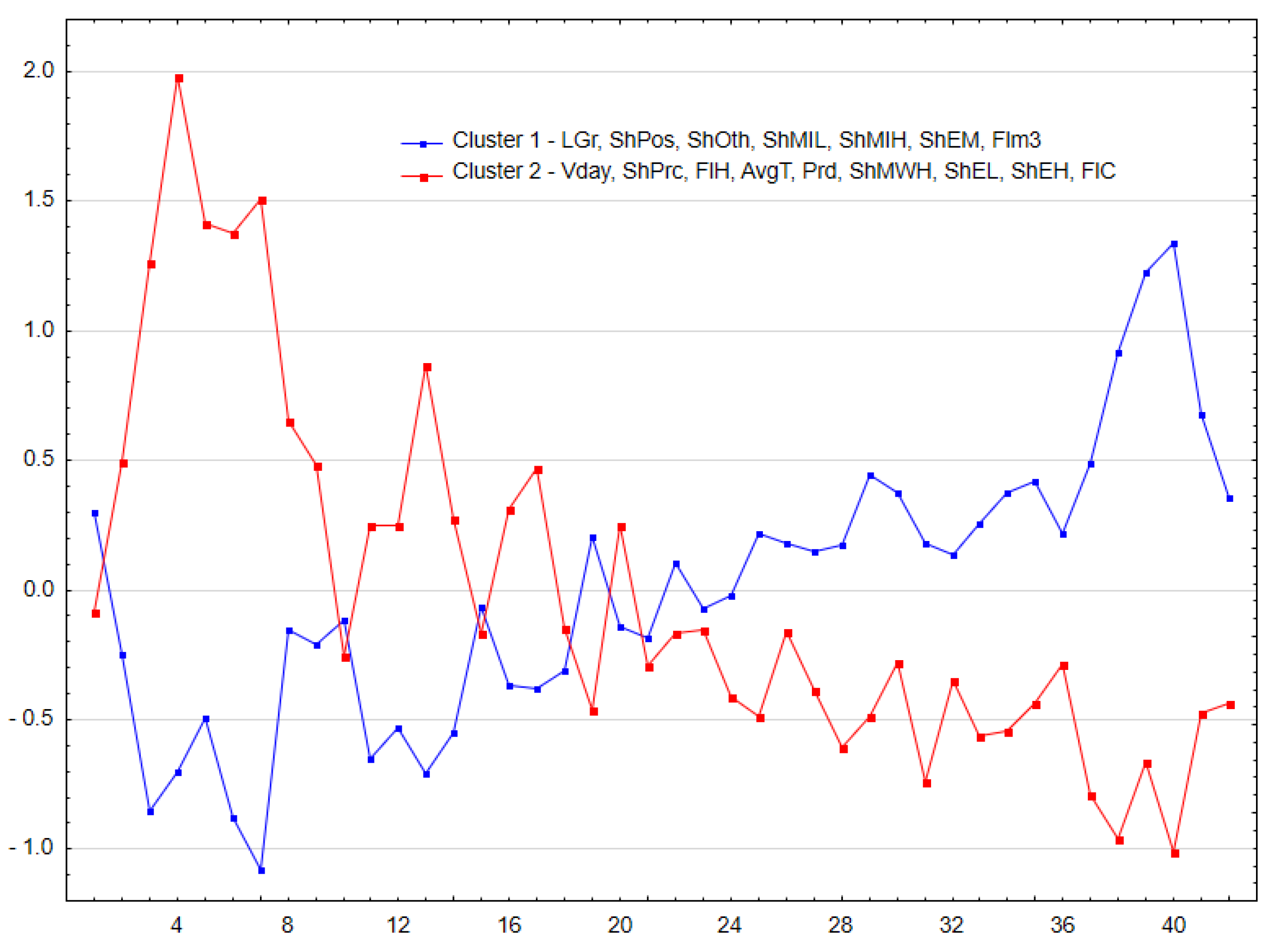
In order to emphasize that workdays within a cluster form distinctive periods, it is also possible to cluster variables for each machine separately and express the result projected on consecutive working days (
Figure 5 and
Figure 6). These graphs show which cluster of variables was dominating each day (the horizontal axis). The composition of clusters for both operators was different: Cluster 1 for machine A consisted of seven variables (the same number as for B), but only three were found for both machines (low gear travel distance (LGr), share of other times (ShOth) and share of machine idling on low revs (ShMIL)). The other variables from cluster 1 for machine A (share of positioning time (ShPos), share of idling on high revs (ShMIH), share of medium engine load (ShEM) and average fuel used per m
3 (Flm3)) were in cluster 2 for machine B.
Figure 5 and
Figure 6 show a definite prevalence of specific clusters in consecutive days (especially evident for machine A), which means that variables from this particular cluster were more pronounced (more distant from the mean) in this period.
3.4. Principal Component Analysis
Principal Component Analysis facilitates the interpretation of which groups of variables (components) affect the process the most; therefore, it is often used in reducing dimensionality. Data from the harvesters were condensed to four main principal components that in both cases explained over 89% of overall variability (
Table 2). For each variable, the component with top weight was bolded. This shows that most variables had their peak in PC1 for both machines (10 in machine A and 8 in B), but with only six that were common. Remarkably, the direction of all the common variables with peak weights in PC1, was completely reversed between the machines: whenever in machine A weighting was positive, the same variable in machine B had a negative weight. In PC2 and PC3, there was only one common variable each, again with the opposite sign.
The loading plot graphically shows the strength and direction of each variable’s influence on the first two principal components. The closer the points are to the perimeter of the circle, the greater the impact on principal components, while points being close to each other indicate variables that correlate.
Figure 7a shows the loading plot for machine A, with visible grouping of five variables in quarter I (positive correlation with both PC1 and PC2) and grouping of three variables in quarter II (negative correlation with PC1, but positive with PC2), quarter III (negative with both components) and quarter IV. The loading plot for machine B (
Figure 7b) presents less conclusive results. Points are closer to the center (which shows lower contribution) and more dispersed. Only two clear groups are recognizable: five variables in quarter III, and five less obvious variables in quarter II. These plots also reveal that the direction of common variables on PC1 is reversed between the machines: total volume harvested per day (Vday), productivity (Prd), fuel consumption per hour (FlH) and per cubic meter (Flm3), share of work time when the machine was idling on high RPMs (ShMWH) and share of work time when the engine worked at a high load (ShEH) are in opposite quarters for machine A (
Figure 7a) and machine B (
Figure 7b).
Results of regression showed that the main factor affecting fuel consumption per cubic meter was average tree size, while for productivity apart from tree size, a share of processing time was significant. Fuel consumption per hour was affected not only by these variables, but also by the distance driven in a low gear, share of time spent idling on low RPMs and share of time the engine was running at a high load. Variables selected by dendrograms as most divisive were volume cut per day, daily fuel consumption and share of time working on high RPMs. K-means divided variables into two clusters that were more prominent each day. Days with the same dominating clusters formed series of consecutive days, which might indicate, for example, a shift in working conditions. PCA explained almost 90% of variance in the first four principal components for both machines. However, an opposite sign in common variables in PC1 for both machines shows an opposite influence of these variables on the production process.
4. Discussion
Data recorded automatically by the control system of machines provide a wealth of information that could be analyzed using conventional statistical methods and modern data mining methodology. Results of such studies are available, but as the modeling approach, study goals and data collected vary, direct comparisons need to be made with caution. Some variables used in this study have not yet been studied or it was not conducted using these methods, hence discussion with other authors is not always possible. On the other hand, some variables have been studied extensively, especially the ones measurable applying conventional methods. Variables with a significant impact on the results were different in various methods (
Table 3). Some variables proved to be significant for both machines (AB), or only for one (A or B). In the case of regression, the variables with significant coefficients are shown. Variables separated as stand-alone in the dendrograms showed the highest dissimilarity with others that clustered into groups. This means that these variables influence the separation the most. The column with k-means shows variables that deviated more than 50% from the mean, thus affecting the clustering into distinctive clusters most significantly. Results of the Principal Component Analysis for the two most influential components, PC1 and PC2, show in which of these a given variable had the greatest weight. This shows their relative importance in describing the work process of a tree harvester, even if their directions (signs) were opposite. Some variables, such as average tree volume or proportion of shift time spent idling on low RPMs or working on high RPMs, are obvious for describing the performance of any machine. Data from the harvester control system enable easy analysis of machine utilization times. Other important variables made available in this way are times that the engine is subject to low, medium or high loads. As seen in
Table 3, these describe the harvester work significantly; yet, due to technical constraints, they are rarely seen in scientific publications.
Total work (shift) time proved to be around 8 h, which is assumed to be a standard working shift time worldwide [
46]. However, some shifts extended this standard considerably, especially in the case of operator B. While this is considered rather usual for forestry workers [
47], increased fatigue can lead to decline in productivity [
48].
Productivity, expressed in m
3 per productive hour, was mostly affected by average volume of tree, which confirms the findings of other authors [
9,
10,
15,
16,
49,
50,
51]. Average productivity (9.98 m
3/h) was lower than that reported by other studies. Using the model developed by Kärhä for Nokka and Timberjack harvesters in second thinning [
49], expected output for an average stem size of 226 dm
3 would be around 16.8 m
3 per operating hour (E15). Similarly, models proposed by Nurminen [
51] would yield around 20 m
3 per gross-effective hour for average stem size obtained in this study. On the other hand, results of a study conducted in the northern European part of Russia [
10] for clear-fells, with trees of average stem size between 0.28 and 0.38 m
3, suggested average productivity of 10.7 m
3/PMH. This is only slightly more than the results of this study, especially considering that the prevailing cutting category in this study was thinning, which naturally lowers the performance [
16].
Proportion of time spend on positioning, processing and other tasks may be measured in conventional time studies. However, it is time-consuming, prone to error and only possible within a limited study time. Automatic recording made it possible to estimate these times for extensive time periods with high accuracy and consistency. In clear-cut areas travelling in a low gear, positioning of the harvester head and felling cut took approximately 30% of the harvesting cycle, while processing accounted for around 70% with the average tree volume of 0.364 m
3 [
52]. Other studies in clear-fell sites with similar tree sizes (0.31 m
3 on average) showed a proportion of stem processing machine hours in productive machine hours to range from 17 to 45% (mean 34%) [
10]. Working in thinning causes more time spent on careful positioning of the harvester head and moving the crane between the residual trees. Studies conducted in thinnings, with smaller machines, reported the proportion of processing time to be around 27% and positioning close to 70% [
51], or in the range of 29–37% and 56–68%, respectively [
49]. These results are close to the ones obtained in this study (27.6% processing time, 52.6% positioning). It is important to note that most results are based on conventional time studies [
49,
52], on the analysis of StanForD files [
16], sometimes assisted by some other time measurements [
6,
51] and only recently focusing on the application of JDLink software [
10,
37]. These methods may be based on slightly different definitions of various work tasks and need some caution when directly comparing results [
6].
Fuel consumption is a natural performance indicator of the operator and the machine. A good operating technique and proper planning may make a difference in fuel consumption even under identical working conditions. In case of this study, hourly fuel consumption was significantly different between the machines (A–14.7 L/h, B–12.3 L/h), but relative fuel use per cubic meter was not significantly different (A–1.30 L/m
3, B–1.36 L/m
3). Similar to productivity, working in thinning affects fuel consumption negatively, as work is more complicated and tree volumes are lower [
32]. According to the measurements made for final felling, the most important factor responsible for increased fuel consumption is working at high engine revolutions and, for the moving phase, the driving speed [
32]. Fuel consumption in clear cutting, as reported by [
52], was higher per hour (21.04 L/h), while lower per cubic meter (1.13 L/m
3), which could be explained by the use of a harvester of a slightly larger size class (Valmet 911.4) with a 170 kW engine. A similar-sized harvester in a Latvian study [
53] had fuel consumption in the range of 16.75–18.2 L/h. Using big, tracked harvesters in South African pine clear-fells gave an even lower fuel consumption rate at 0.64 L/m
3, while using 23.55 L per hour, which can be explained by achieving very high productivity of over 54 cubic meters per hour [
54].
Factors influencing fuel consumption included mostly average tree volume, which corresponds with results reported by other authors [
32,
52,
55]. Interestingly, when considering fuel consumption per working hour, another factor became relevant, i.e., distance driven in a low gear. This confirms that increasing the need for machines to drive more considerably affects average hourly fuel usage. Additionally, the proportion of engine time at different load levels turned out to be a significant factor for one of the machines. Notably, the engine load level did not have a significant impact on fuel use per cubic meter. This could be explained by the fact that when the engine runs at a higher load, greater productivity is achieved, which offsets the higher fuel consumption per unit of time. Such analyses are rarely made, as data on engine load are difficult to obtain. Results by [
54] reported no influence of tree size and driving distance on fuel consumption for harvesters; however, this was mainly due to the limited variation in tree size, and lack of direct measurements of travelling distance.
Driving distance has usually been measured and analyzed regarding forwarder work, where it is one of the most important factors affecting productivity [
52,
56,
57,
58,
59]. Little is known about distances driven by harvesters during work. Kärhä [
49] reported that harvesters in second thinning spend around 21–27% of work time moving (driving between subsequent work positions). In a similar fashion, Nurminen [
51] assigned between 14 and 26% (mean 20%) of total effective working time to the moving phase in thinnings. Taking into account the driving speed in a low gear around 5 km/h, driving on average 6.3 km (machine B) to 7.9 km (machine A) takes 1.26 h and 1.58 h, respectively. This, in turn, corresponds to 14–20% of work shift time for each machine. As analyses of fuel consumption proved, the distance driven in a low gear each day was one of two factors significantly affecting hourly fuel consumption. The distance driven in a high gear usually corresponds to moving between work sites, and should be monitored in order to avoid excessive wear of hydrostatic transmission components. It is not advised to drive more than 15 km at one time and both machines generally tended to travel shorter distances.
Machine utilization times recorded automatically, revealed that most of the work time (68–80%) is spent working on high RPMs, and idling on low RPMs took on average around 15% of the workday. Due to some irregularities in the operators’ habits, a significant difference in time spent with the engine off was found. The operator of machine B was accustomed to taking the key off the ignition during breaks, thus interrupting the time measurement. This resulted in only several minutes per day registered as a time with the engine off (3.6 min on average), in contrast to machine A with the average of 64.8 min. Such customs must be taken into consideration when conducting wide range studies and drawing conclusions, as these can affect the data quality, even though these times are recorded automatically and with high precision.
Data concerning the level of engine utilization while working are new to the analysis of harvester work, as these may not be recorded using traditional methods. Automatic data collection, based on the internal computer system, makes it easy to gather information on the load exerted on the engine as a result of work conditions. As this load level is not directly controlled by the operator (in contrast, e.g., to RPMs) it gives an overview of the effect that the workload has on the engine. Although a proportion of work time with a high engine load was relatively low (6–9%), it proved to be a significant factor influencing hourly fuel consumption. As the analyzed machines spent most work time at a medium or low engine load, it could be concluded that their utilization was below optimum. It should be expected that during most of machine work time the engine would be at a medium or high load, as this would mean higher productivity (the correlation coefficient between productivity and time of high engine load was 0.79 for machine A and 0.91 for machine B).
Dendrogram group variables that are most similar to one another. Notably, in the case of both machines, the variables that were closest to each other were fuel used per one cubic meter and average tree size. Variables that cluster together with productivity are usually common between two machines, with the exception of share of time used for ‘other’ tasks (i.e., not positioning or processing). Variables significantly affecting fuel use per hour, as established with a linear regression, were in the same cluster in the case of machine B, while for machine A, only four out of seven were clustered together.
A similar goal of grouping variables that describe the process in a similar way might be achieved by the k-means method. Most variables that had the greatest influence on clustering into two groups (productivity, average tree size, fuel use per m
3 and share of time with high engine load) were in the same cluster when grouped by dendrograms. The only exception was the total volume per day that was a standalone variable in dendrograms. Characteristic streaks of consecutive days, where variables of a certain cluster were prevailing, probably indicate work under different conditions—different stands, cutting type or assortments. Although clearly visible on graphs (
Figure 5 and
Figure 6), this interpretation would need a confirmation in follow-up studies. The potential use of such analyses would be to detect anomalies.
Principal Component Analysis reduces the number of variables to new artificial variables—components that explain most of the variation while not being correlated. Ideally, the variables that have the highest weights in a certain component form some logical group that can be interpret together, as was studied by Palander [
6]. This was not feasible in this study due to discrepancies between the machines and also due to fact that the most important variables were not closely logically connected. An interesting feature of PCA performed for the machines separately is that the variables in PC1 that were common in both machines have an opposite effect. The ones with the positive sign in machine A had the negative sign for machine B, and vice versa. This proves that the operator effect is a considerable factor and can affect the results in a different manner due to personal habits and traits.
5. Conclusions
Automatic data collection from operating systems of harvesters and other advanced forestry machinery is a promising method of acquiring knowledge on the timber harvesting process. However, it involves some challenges when it comes to handling extensive data. Data mining techniques assist in analyzing various metrics for the extraction of information that can be valuable both for practice and science. This method of data acquisition comes with many advantages, such as accuracy, low cost, easy storage and access, to name a few. Automatic recording without human involvement makes it possible to lower the cost [
13], avoid human mistakes [
6] and prevent Hawthorne’s effect [
11,
16,
37]. On the other hand, some of these benefits may also lead to disadvantages, such as an extensive amount of data that is hard to comprehend by humans, some irregularities depending on software versions or on human actions. In this study, data were obtained from mid-size John Deere harvesters through the JDLink internet service to keep the records consistent. The assumption of this study was to use only data available from the JDLink, without supplementing with any other records. This limited the methods used to traditional linear regression and unsupervised learning, such as clustering with dendrograms, k-means or PCA. Extending the database with data from the forest inventory, some GIS layers, or records from the harvesting company, would also lead to extension in the range of used methods [
2]. The scope of this study was to show the applicability of methods to analyze data that were already available, with minimum transformations (although some were necessary). Conventional linear regression made it possible to extract variables influencing productivity and fuel consumption per hour, while for consumption per cubic meter, a logarithmic model had to be developed. Clustering with dendrograms showed grouping of variables most closely related to one another. The results recorded for two separate machines showed comparable clustering, which confirms applicability of this method. Splitting the observations into two clusters with the k-means method gave similar results as dendrograms, where the most important variables end up in the same cluster. More interestingly, the timeline of clusters’ averages showed a clear distinction between longer periods (days) that suggest changes in working conditions. This could be used to automatically detect anomalies—for example, a change of cutting type or operator change—after the accuracy is checked by the follow-up study. Analysis of the principal components proved to be problematic in this case. On one hand, for both machines, it achieved good accuracy—the first four components explained a total of 89% of variability. On the other hand, the nature of the variables’ influence was completely different between the machines (reverse signs), which renders the results unfit for generalization.
This study will be followed by a field study to assess the accuracy and collect data that would enable supervised learning and prediction techniques, as missing data regarding cutting category or stand characteristics limited the possible analytic methods. Another limitation is connected with the dependence on the manufacturer’s proprietary software, which only allows to use John Deere harvesters, and demands subscription to the JDLink service. Although other manufacturers supply similar software, the available data might be structured differently and comparisons might be impossible. Finally, this method of data collection only works on relatively new machines and requires the machines to be equipped with a GSM modem. Often mentioned disadvantages of machine learning models include their rather low interpretability and sometimes confusing architecture, which hinders their widespread application [
16]. Still, the expectations of the business environment and the great potential of “big data” techniques in forestry will likely lead to a rapid development in this field [
2,
4,
16,
25]. Therefore, future research should be focused on improving the applicability, extending the analyses to the whole harvesting team (the harvester and the forwarder) and providing exact predictions.


