Article

Variability in Snowpack Isotopic Composition between Open and Forested Areas in the West Siberian Forest Steppe

1
Faculty of Geography, Lomonosov Moscow State University, 1 Leninskie Gory, Moscow 119991, Russia
2
Institute for Water and Environmental Problems SB RAS, 1, Molodezhnaya Street, Barnaul 656038, Russia
*
Author to whom correspondence should be addressed.
Forests 2023, 14(1), 160; https://doi.org/10.3390/f14010160
Submission received: 23 November 2022 / Revised: 12 January 2023 / Accepted: 13 January 2023 / Published: 16 January 2023
(This article belongs to the Special Issue Forest Ecohydrology: From Theory to Practice)

Abstract

:
The stable water isotopes in snow (primarily 18O and 2H) are widely used for tracing hydrological and ecological processes. However, isotopic signatures of snow can be significantly modified by topography and land cover. This study assesses spatial and temporal variability of the bulk snowpack isotopic composition (δ18O, δ2H, d-excess) between forested (pine and birch) and open areas in the West Siberian forest steppes. Isotopic samples were collected over the peak snow accumulation in 2017–2019. The snow isotopic composition within forested areas differed from open steppes, mainly in reducing d-excess (1.6‰ on average). We did not find a significant effect of canopy interception on snow enrichment in heavier isotopes. Snowpack in the pine forests was even lighter by 3.6‰ for δ2H compared to open areas, probably, due to low energy inputs and interception capacity. Additionally, snow depth significantly influenced the isotopic composition spatial variability. As snow depth increased, δ18O and δ2H values decreased due to conservation within the snowpack and less influence of sublimation and moisture exchange with the soil. However, this pattern was only evident in winters with below-average snow depth. Therefore, taking into account snow depth spatial and seasonal variability is advisable when applying the isotopic methods.

1. Introduction

Snow accumulation, storage, and melting dynamics affect multiple hydrological, ecological, and social processes in mountainous and high-latitude environments [1,2]. Tracking changes in snowpack accumulation and melt rates is challenging because the driving factors operate at multiple spatial and temporal scales [3,4,5]. Stable water isotopic composition of snow (primarily δ2H and δ18O) has become a valuable tool for investigating various snow hydrological and ecohydrological processes [6]. Implementations include snow contribution to groundwater recharge [7,8], streamflow generation during rain-on-snow events [9,10], exploring vegetation water sources [11,12,13,14], etc. However, the application of isotopic methods is complicated by snow evolution processes that alter the isotopic signal [15,16,17].
Snow mass and energy balance is altered by complex processes such as sublimation, wind redistribution, forest canopy interception, melting, and metamorphism [18]. Since snow contains liquid, solid, and vapor phases, most of these processes are accompanied by phase transitions, changing the stable water isotopic composition [6,19,20]. The intensity of snow hydrological processes varies in space. Spatial factors affecting snow isotopic composition have included altitude [21,22,23], aspect [15,24], snow depth [21], and canopy interception [25,26,27]. Most of these factors affect snow sublimation fluxes, which leads to enrichment in heavier isotopes of the remaining snow cover [16,22,28,29].
Forest canopy interception affects the snow isotopic composition by increasing the sublimation of intercepted snow and making throughfall isotopically heavier [6]. The under-canopy snowpack in the north-western US was up to one-fourth smaller and isotopically heavier by roughly 2‰ in δ18O compared with the snowpack in the clear-cut area [26]. Studies in Switzerland showed that the isotope ratios were higher in the snowpack under forest canopy than in open grasslands (by 13.4 ‰ in δ2H and 2.3 ‰ in δ18O) [27]. However, a five-year study in the southwestern US has shown a much more significant influence of snowfall isotopic input and aspect on δ18O than canopy density [28]. Additionally, several mechanisms of changes in the snow isotopic composition in complex landscapes remain poorly understood, such as the effect of wind redistribution [6].
Most of the works cited above were performed in mountain forests in relatively humid regions of Europe and North America. Over Siberia, studies have shown that the variability of the contribution of many precipitation sources to the snow results in large isotopic variability [30,31]. At the same time, more detailed catchment-scale studies investigating changes in snow isotopic composition have not been conducted either in the boreal forest area or in the forest steppe.
Snow in continental semi-arid regions is the major water source for ground and soil water recharge and streamflow generation [32]. Considering the significant differences in the snow isotopic signal compared with rainfall, implementation of the isotopic methods for tracing streamflow formation, groundwater recharge, and plant water use seems promising in these regions. However, the mechanisms of the snowpack isotopic composition spatial variability and post-depositional fractionation remain poorly understood. In this work, we focused on changes in the stable water isotopic composition of snow (δ18O, δ2H, d-excess) between open and forested areas during peak snow accumulation over three years (March 2017–2019). The studies were conducted in the Kasmala River basin located in the forest steppe ecoregion in the south of Western Siberia. The basin structure consists of extensive arable lands, Scots pine forests, and small patches of deciduous forests. Basin landscape composition allowed us to study changes in the snow isotopic composition in open and forested areas and to evaluate factors influencing isotopic ratios considering the differences in topography and seasonal climate.

2. Materials and Methods
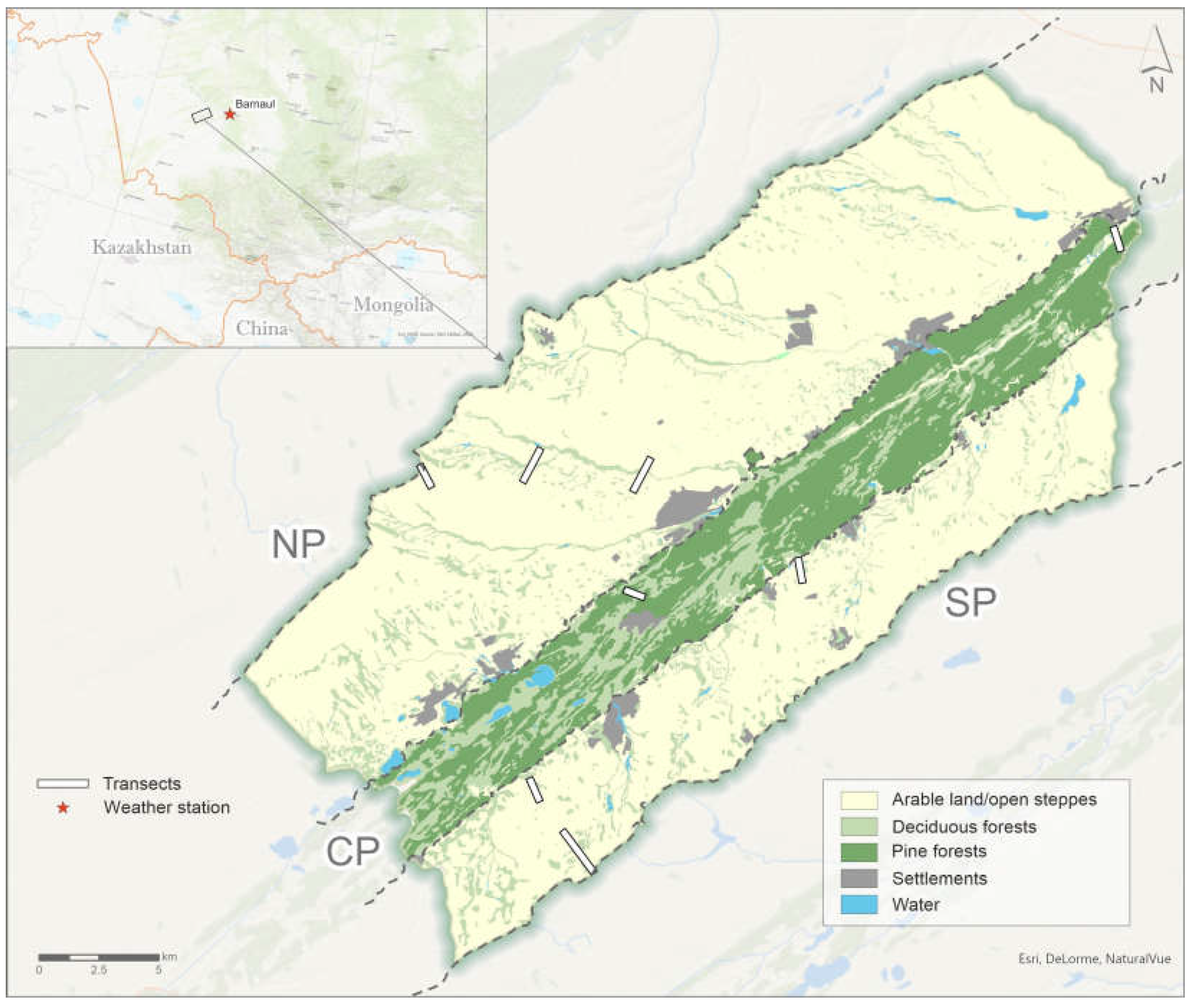
2.1. Study Area

We carried out the study in the 1768.7 km2 Kasmala river basin (53°4’ N, 82°20’ E) in the south of the West Siberian Plain (Figure 1). The Kasmala basin is a snow-dominated watershed in the headwaters of the Ob River.
The study area belongs to the West Siberian forest steppe ecoregion [33]. This region is also part of the West-Siberian grain belt, an important agricultural region in southern Siberia. The dominant land cover type is arable land (59.7%). A unique characteristic of this part of the West Siberian Plain is the long strips of Scotch pine (Pinus sylvestris L.) forests [34,35,36]. This forest type (covers about 12%) is characterized by dense pine stands (canopy density 60–80 %) with a small proportion of mixed deciduous vegetation. The average diameter at breast height is about 25–30 cm, and tree height is between 20–25 m. The forests occupy the sandy massifs within the extended ancient flow depressions. Upland slopes oriented towards the depressions have small slope angles (1–3°) covered by arable land and steppe patches. Another type of forest presented here is the small patches of birch (Betula pendula Roth) and aspen (Populus tremula L.) stands (5.9%). The basin is naturally divided into three main parts: the northern (NP) and southern (SP) open steppe areas with deciduous forest patches and the central part, occupied mainly by pine forest (CP). Additionally, in the study, we considered arable land/open steppes, deciduous forests, and pine forests as three major land cover types.
Continental climate with strong seasonality in the study region varies from sub-humid in the northeast to semi-arid (steppe) in the southwest. The area has cold winters and hot summers with a mean annual temperature (1966–2020) of 2.4 °C at the Barnaul weather station (53 km to the nearest transect) [37]. The average annual precipitation is 427 mm. The mean winter (November-March) precipitation is about 125 mm. Wind drift is the most crucial factor in snow redistribution. The average daily wind speed in November-March is 2.7 m/s [37].

2.2. Sampling and Laboratory Analysis

We conducted three field campaigns around 10–15 March, 2017–2019 during the peak snow accumulation. Sampling was performed along eight transects that varied in length from 500 m to 2 km. The distance between measurements was 200 m in open areas and 100 m in forested areas. NP and SP included three transects each, and CP included two transects (Figure 1). Each transect differed in terrain characteristics (ruggedness, slopes, and aspects) and land cover composition (open areas, deciduous, and coniferous forests). GPS location of each sampling point was recorded. During the field campaign, the bulk snowpack samples were collected at each location using a 60 cm snow coring sampler VS-43. The samples were weighed to obtain bulk density and calculate snow water equivalent (SWE). Then, the entire samples were immediately placed into sealable high-density polyethylene bags to prevent further evaporation and fractionation effects. The snow depth was measured at the same points using a special snow ruler. If the snow depth was higher than 60 cm, the snow was measured successively from deeper layers. A total of 192 samples were taken over three sampling years.
Snow samples were brought to the laboratory in sealed bags on the day of sampling and melted at room temperature. Once the samples completely melted, they were filtered through 0.45-μm filters (Minisart NML Plus) into 2-mL glass vials. The isotopic composition (δ18O, δ2H) of all samples was analyzed through laser spectroscopy (PICARRO L2130-i (WS-CRDS). The measurement uncertainties were ±0.4‰ for δ18O and ±0.1‰ for δ2H. Water samples were calibrated against the international standards (V-SMOW, GRESP).

2.3. Data Processing and Analysis

We analyzed spatial and temporal variations in the bulk snowpack isotopic composition. In exploring interannual differences, we considered variations in temperature, precipitation, and snow accumulation relative to the interannual means from the Barnaul weather station [37]. The station is the closest to the study area (53 km to the nearest transect) and has the most consistent series of observations.
The δ18O and δ2H mean values among basin parts, land cover types, and sampling years were tested using non-parametric Kruskal–Wallis H test. Additionally, Wilcoxon test with the Bonferroni correction was applied to evaluate the differences between the group levels.
For assessing the site-specific covariation of hydrogen and oxygen stable isotope ratios, we created δ2H vs. δ18O plots (similar to local meteoric water lines) for the basin parts (NP, CP, and SP). Additionally, the second-order isotopic parameter deuterium excess was computed (d-excess = δ2H – 8 ×δ18O) [38]. D-excess helps distinguish equilibrium and nonequilibrium processes through the differences from the global meteoric water line (GMWL; δ2H = δ18O + 10) [39]. Values less than 10‰ often indicate kinetic fractionation due to evaporation or sublimation [6].
In order to assess the interactions between isotopic composition, topography, and land cover, we created a set of multiple regression (MLR) models. Stepwise regression analysis was performed separately for δ18O and δ2H as dependent variables. However, the relationships behaved similarly, and we used δ2H for further analysis due to a smaller measurement error. All variables were first tested for normality of distribution, multicollinearity, and the presence of outliers. We also calculated Z-scores for the predictors and response variables of the final models. The selection of variables for each model was performed automatically by stepwise backward elimination according to the Akaike information criterion (AIC). Finally, each final model was checked for residual distribution and homoscedasticity.
Input variables were chosen based on their potential effect on the isotopic composition of a bulk snowpack. Snow depth and SWE were used as indicators of wind redistribution since wind is the main factor of depth and SWE spatial heterogeneity on the plains (no elevation gradient). Given that depth and SWE are correlated, they were included in the regression separately. The snow energy balance and, therefore, the processes of sublimation and melt depend on the local topography. The slope, aspect, general curvature, and Topographic Ruggedness Index (TRI) were calculated using the SRTM digital elevation model (DEM) [40]. The aspect was transformed with the cosine function, resulting in a value of −1 for north- and 1 for south-facing points. We used the land cover map based on the Landsat satellite images to calculate the forest ratio in the 200 m surrounding the sample points. This metric was chosen because forests in the study area affect snowpack accumulation not only via canopy interception but also through the obstruction of wind redistribution. The obstruction factor appears mainly in the deciduous forest patches within the steppes.
Statistical analysis was performed in R (http://www.r-project.org, accessed on 27 March 2021). Topographic variables were calculated using QGIS (www.qgis.org, accessed on 2 June 2021).

3. Results

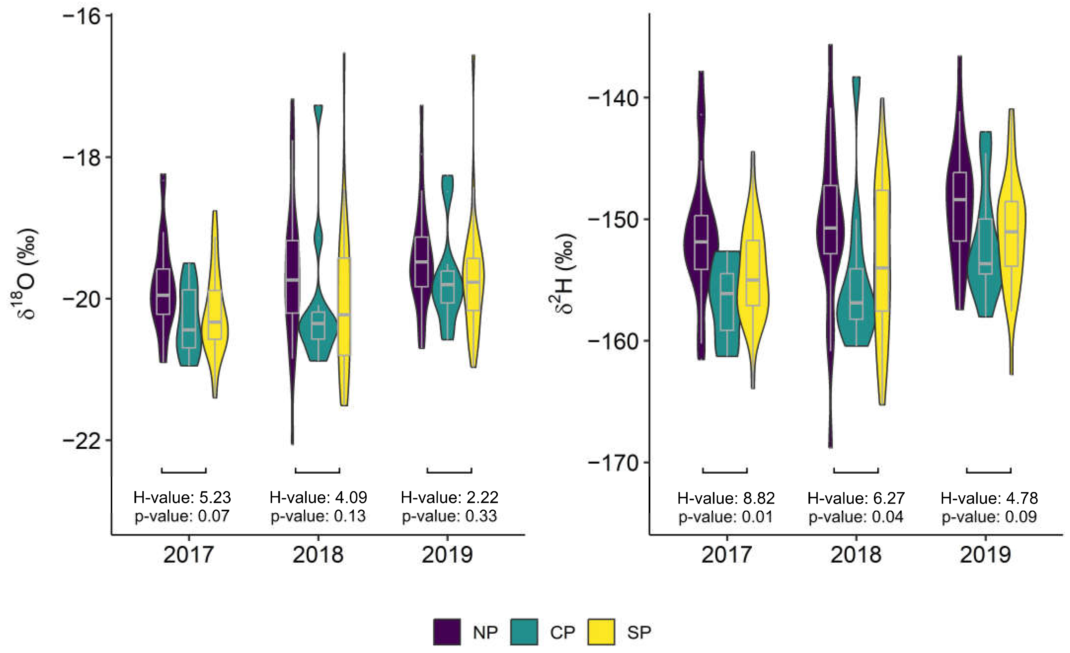
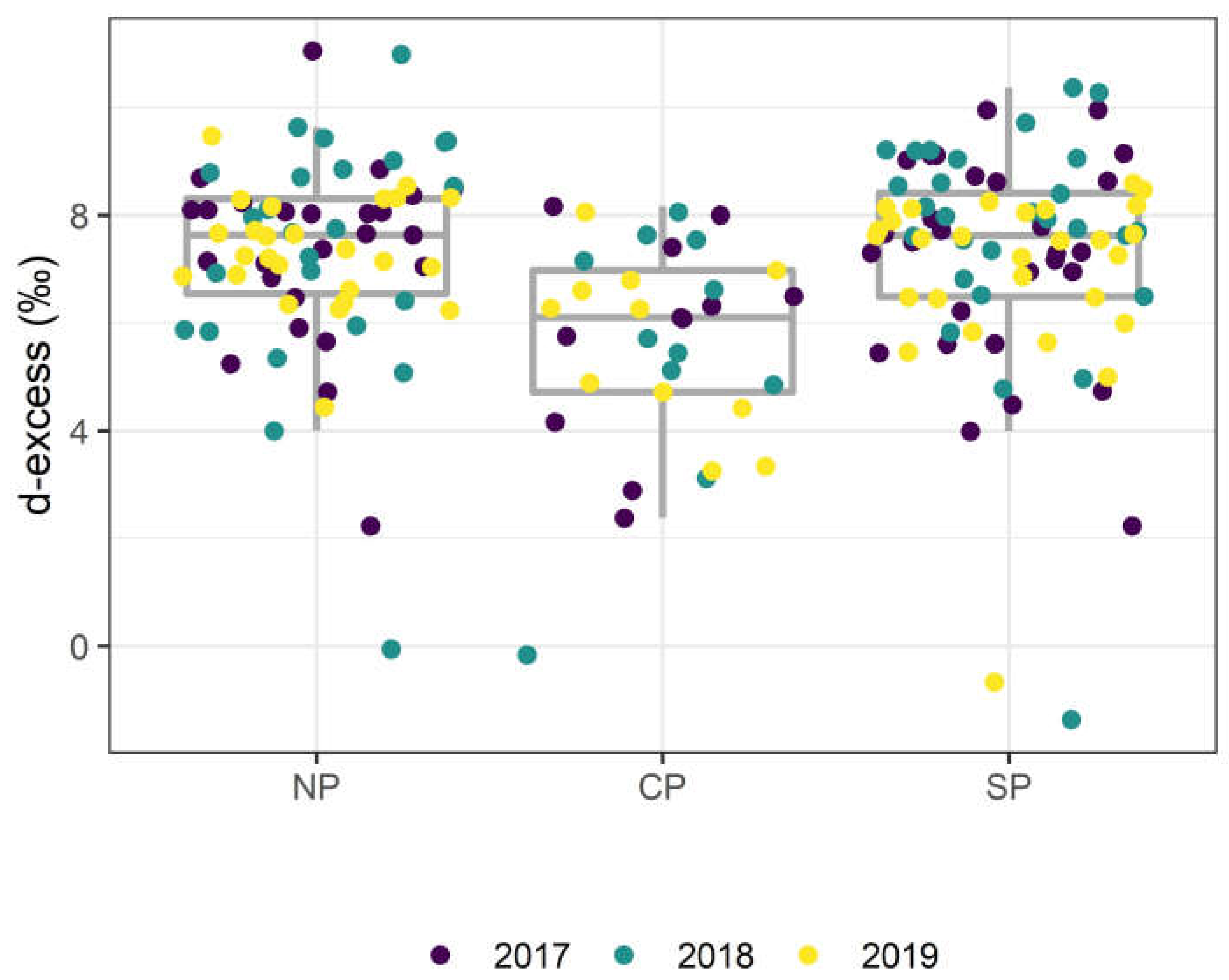
3.1. Interannual Differences

Most seasonal climate parameters were close to average during winter seasons 2016/2017–2018/2019, excluding snow conditions. Mean winter temperatures did not differ much from the long-term mean (Table 1). Daily temperatures above 0 °C) were uncommon (for example, in December 2018). However, very low temperatures occurred more frequently, such as in November 2016, January 2018, and February 2019 (Figure 2). Wind speeds in 2016/2017 were close to the mean (2.3 m/s), 2017/2018 and 2018/2019 had lower average wind speeds (1.7–1.8 m/s).
The strongest differences were observed in snow cover dynamics. The maximum snow depth values were above average in 2016/2017 (73 cm) and extremely below average in 2017/2018 (25 cm). March 2018 had the lowest snow depth during the station period of record. Depth and SWE values also varied on our transects during the study period. The most considerable difference occurred between 2016/2017 and 2017/2018, when depth and SWE were 57 % and 70 % lower, respectively (Table 2). Therefore, the studied winter seasons had significantly different snow mass conditions but were relatively similar in other seasonal climate parameters.
According to Kruskal–Wallis test results (Table 3), differences in mean isotopic composition between sampling years were significant. The median levels varied only around 1‰ in δ18O and 4‰ in δ2H during sampling years.
Variability within each sampling year was substantially higher (Figure 3). The isotopic variation had the highest rates in 2018 when the snowpack was extremely shallow. The range reached 6.3‰ in δ18O and 42.6‰ in δ2H. In 2017, the range was approximately half and amounted to 3.2‰ and 26.0‰ in δ18O and δ2H, respectively. The standard deviations (Table 2) of each sampling year also demonstrate differences in variability.
Differences in mean isotopic composition among the northern (NP), central (CP), and southern (SP) parts of the basin were also significant considering the whole study period (Table 3). Firstly, significant differences may indicate expected differences in the drivers of snow isotopic composition: primarily wind redistribution in open areas and canopy interception in forests. Looking at each year separately, the forested and open parts of the basin differed significantly only in δ2H (Figure 3). Additionally, Wilcoxon test showed (p-value < 0.05) that δ18O and δ2H varied significantly between NP and CP-SP.
Differences among land cover types were significant for δ2H and d-excess mean values (Table 3). As in the case of the basin parts, δ2H and d-excess varied significantly between open steppes, deciduous forests, and pine forests (Wilcoxon test p-value < 0.05). Pine forests and deciduous forests were not statistically different.
During the entire study period, the snowpack isotopic composition was slightly heavier within the open parts compared with the forested. The δ18O and δ2H values in CP were on average lower than in open NP and SP, but only by 0.2 and 3.6‰, respectively. We expected higher δ18O and δ2H values in the forested part due to canopy interception. However, no direct effect was observed.

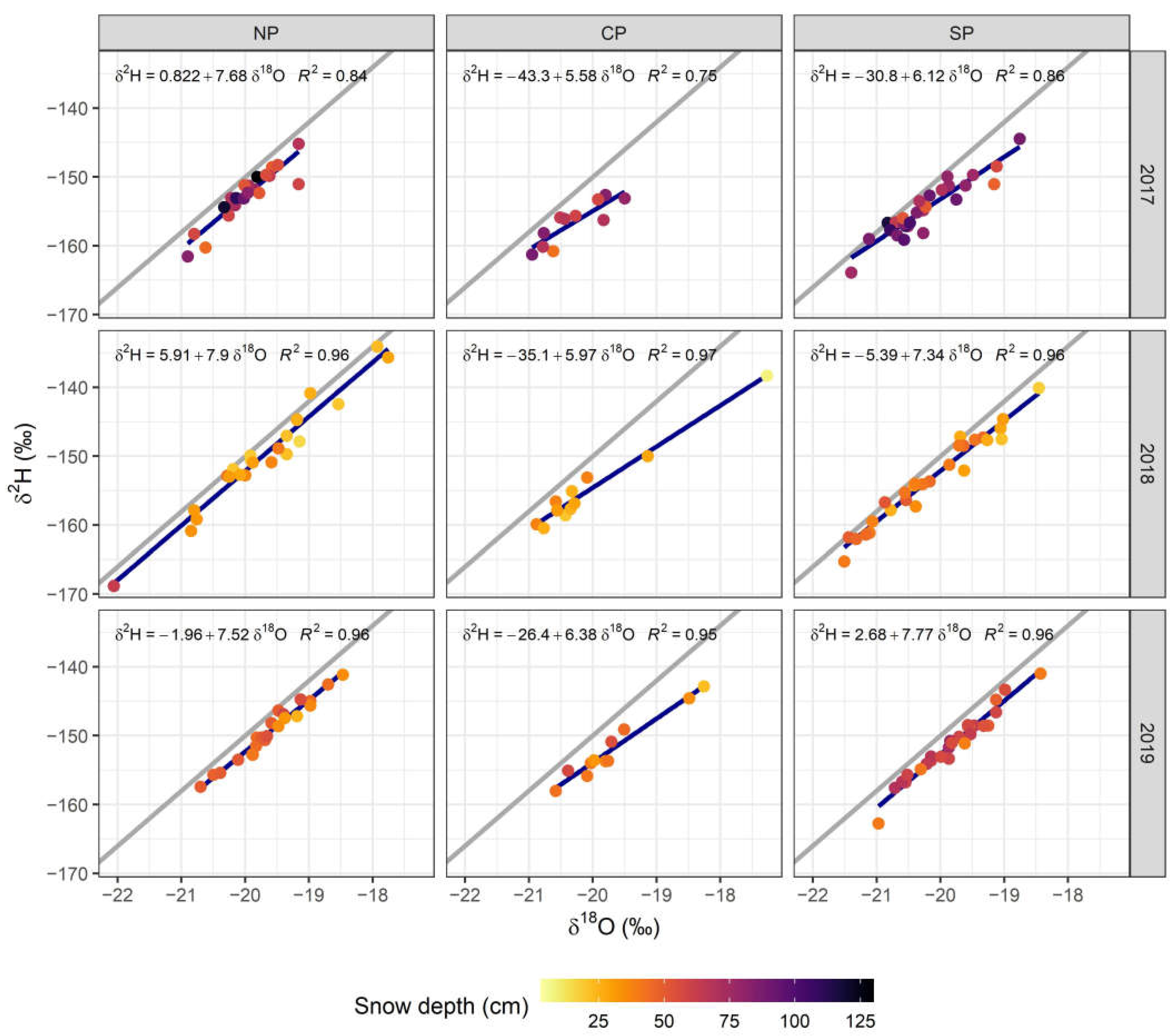
3.2. Oxygen and Hydrogen Ratios

Figure 4 gives an overview on δ2H vs. δ18O relationships among the sampling years and basin parts. All samples lay lower than the GMWL, indicating the influence of nonequilibrium processes (Figure 4). In all equations, slopes were far below 8, and intercept values did not exceed 10, corresponding to the similar parameters of GMWL.
Slope and intercept values of δ2H vs. δ18O regressions showed clear spatial patterns. In the open SP and NP slopes ranged from 7.90 to 6.12. The slope values were significantly lower in the forested part (5.58 to 6.38). Furthermore, the CP intercepts also reached very low values (up to –43.3). This aspect indicated significantly higher sublimation rates and other nonequilibrium processes in the forested part.
Slopes changed little over time, especially depending on the amount of snow each winter season. Only the intercept values changed significantly (by more than 10–20) within the open and forest parts. On the one hand, this may indicate the constancy of fractionation processes on-ground (stable slope), and on the other hand, the influence of snow formation conditions during each winter season (unstable intercept).
D-excess values also showed spatial patterns, remaining relatively stable interannually (Figure 5). CP’s mean d-excess values (Table 2) were 1.6 ‰ lower than open SP and NP. Moreover, the d-excess fell below 10 (d-excess of GMWL) in all parts of the Kasmala basin. According to the Kruskal–Wallis test (Table 3), mean differences were significant across the basin parts during the study period. The major differences occurred between CP and NP/SP (Wilcoxon test p-value < 0.001). The contrast again referred to the high intensity of nonequilibrium processes in the forested part of the basin, which, however, did not lead to direct enrichment in heavier isotopes of the forest snowpack.

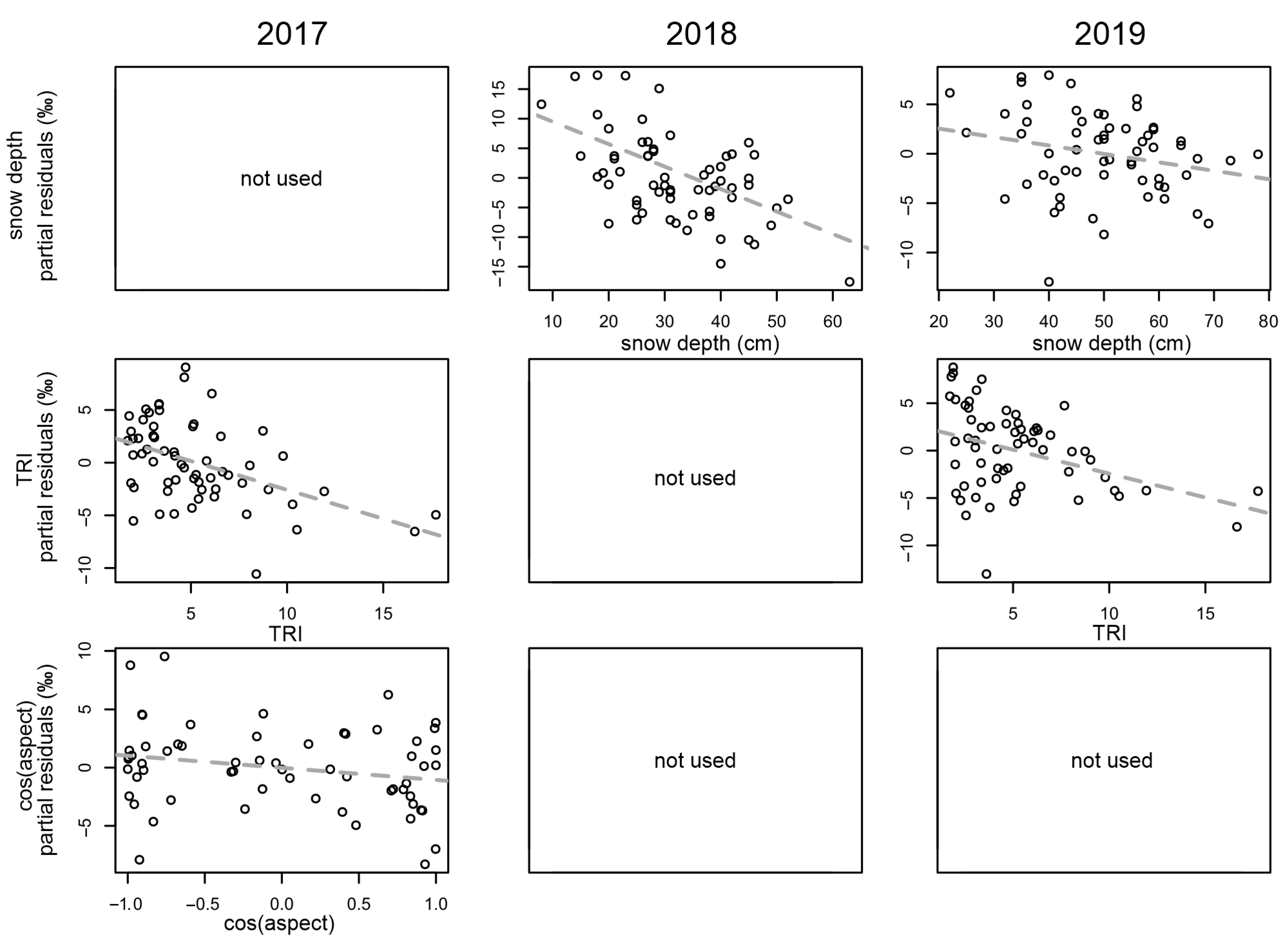
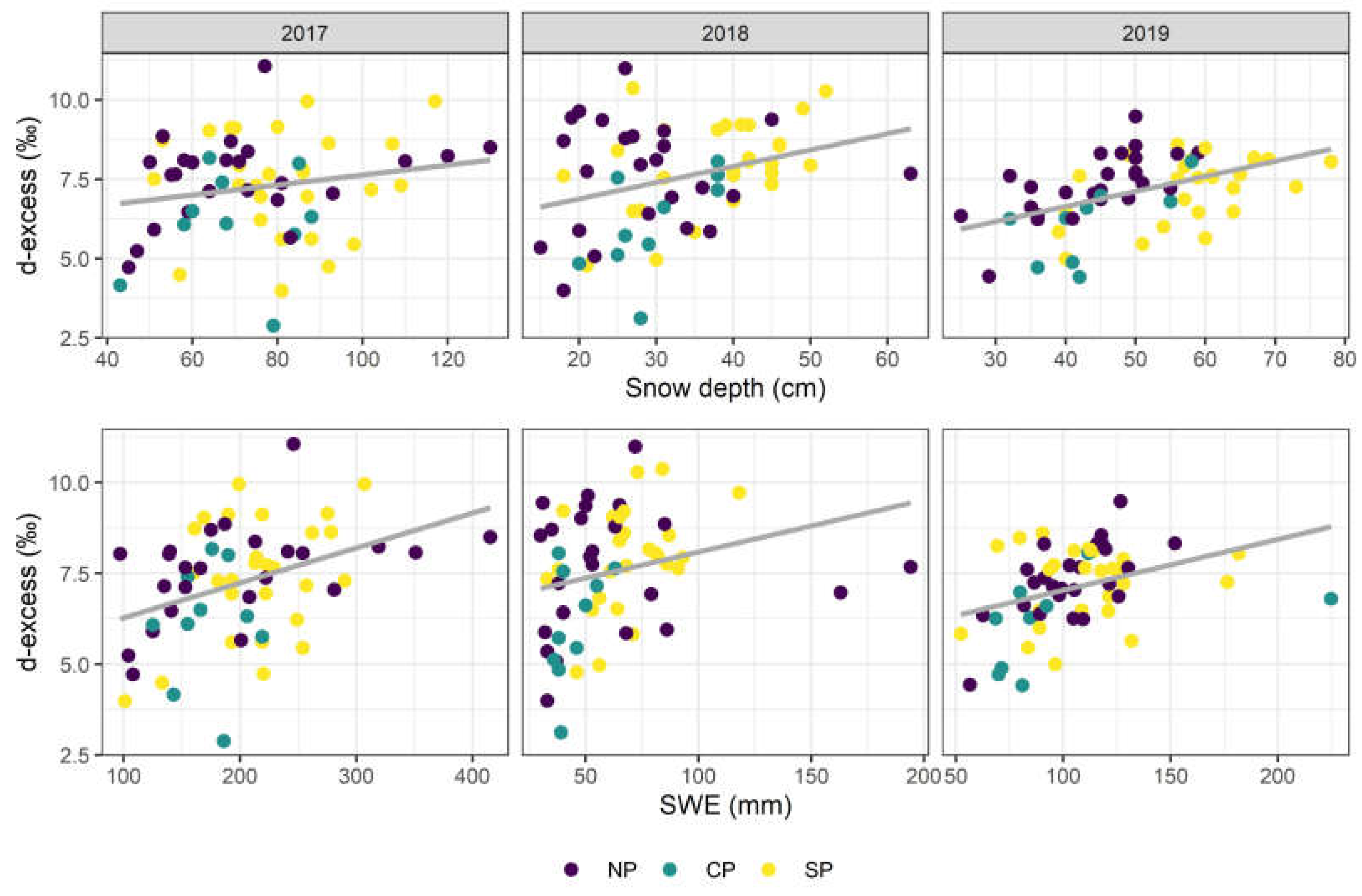
3.3. Influence of Topography and Land Cover Factors

Only snow depth and TRI had a relatively stable effect on δ2H. The influence was evident in two of the three years. The other predictors had no significant influence, except for a feeble impact of Aspect in 2017 (Table 4).
The effect of snow depth was closely related to the snow amount over the sampling years. The influence of depth was not significant in 2017 (high snow). However, in 2018 (shallow snow), the influence of depth became considerable and described almost 32% of the variability. The slope was negative, which means that δ2H values decrease with increasing snow depth. In moderate snow 2019, the influence of depth became weaker. The linear influence of snow depth is evident in the plot of partial residuals (Figure 6).
The TRI effect was most likely related to the wind redistribution of snow from uplands to small valleys. Higher TRI values mean higher ruggedness of the terrain. In the study area, higher TRI values typically belong to river valleys. The coefficients were also negative, indicating a decrease in δ2H values as we moved toward the valleys. TRI was a significant predictor in 2017 and 2019. These winters had above-average snow depths and quite a high wind intensity, especially in 2017.
SWE, as well as forest ratio, did not show any significant effect on the isotopic composition. SWE was included in the models instead of snow depth, but it was significant only in 2018, and the influence was weaker (adjusted R2 was about 0.15). A similar SWE value can be formed by increasing both depth and density, which are controlled by distinct processes from the isotopic composition perspective. The forest ratio also did not play a significant role. We attribute this effect to fundamentally different processes occurring in coniferous (canopy interception) and deciduous forests (obstacle of wind transport). However, the sampling points in these areas may have similar forest ratio values.
The d-excess also showed strong correlations with snow depth and SWE, confirming the isotopic composition-depth patterns (Figure 7). Snow depth and d-excess were positively correlated (Table 5) in 2019 (moderate snow) and 2018 (shallow snow). This relationship weakened in the high snow winter season (2017). The relationship was most stable in moderate 2019, while in 2018 several points deviated from the general tendency. We suppose the deviations were related to some local features of snow stratigraphy that attenuate fractionation despite shallow snow. In contrast to H2, d-excess showed significant correlations with SWE as well (Table 5). However, the strongest relationship was observed in 2019, when the SWE values largely corresponded to the distribution of snow depth. This similarity was largely responsible for the significance of this relationship. In other sampling years, the linear influence of SWE on d-excess was not evident, despite the significance of the relationship (with the presence of outliers and heteroscedasticity).

4. Discussion

The snow isotopic composition showed differences between open and forested areas, mainly in reducing d-excess and the slope of δ2H vs. δ18O regressions. The main predictor connected with snow enrichment in heavier isotopes was snow depth. The effect was especially evident in winter seasons with shallow snowpack.
The slope and intercept of δ2H vs. δ18O regressions corresponded to the values typical for the continental climate [41]. Additionally, the slope and intercept values agreed well with data previously obtained for the same region [31]. Negative intercept values and their high variability are typical for regions with a cold continental climate due to significant differences in the mechanisms of precipitation formation [41]. Under these conditions, the consistently low slope values and low d-excess values in the forest part most likely indicate the influence of sublimation.
The effect of canopy interception on the isotopic composition was observed not in the direct enrichment in heavier isotopes but through a decrease in d-excess. This pattern slightly differs from the existing studies in which the enrichment in heavier isotopes was correlated with increasing canopy density [26,27]. However, a recent study has shown that canopy density may not have a statistically significant influence on the spatial variability of δ18O [28]. Forest d-excess may be lower than in open areas (in [27], d-excess was not given but could be calculated from the average δ2H and δ18O values) or almost independent of canopy density [26]. We suppose that the lack of direct enrichment occurred due to the lower interception capacity of pine forests and low energy inputs for sublimation. Compared to fir and spruce forests, snow interception, and sublimation losses in pine forests may be up to 10% lower [42], despite the slightly longer deposition of snow on the canopy [43]. The work [27] noted slightly smaller interception effects on isotope ratios at the high-elevation transect, which the authors attributed to lower energy inputs. In the cold continental climate of southern Siberia, this factor may also limit sublimation.
The influence of snow depth on the isotopic composition was the most critical factor of both spatial and temporal variability. Previously, it has been shown that the upper and lower layers of snow are sensible to the changes in the isotopic composition due to the influence of melting, sublimation, and moisture exchange with the soil [6,20,28,44,45]. Vapor flux from the lower snow layers to the upper ones (due to the thermal gradient) usually does not significantly change the isotopic composition since all changes occur within the snowpack. These processes contribute to the homogenization of the isotopic composition between the individual layers during the winter [31,46]. In shallow snow conditions, bulk snowpack isotopic composition is much more sensitive since the upper and lower layers constitute a significant part of the snowpack. In the areas with increased snow accumulation (high snow depth), the fraction of “stable” snow within the snowpack is higher. Such snowpacks tend to be isotopically lighter. In moderate snow winter seasons, the isotopic composition-depth relationship weakens, but it is still recognizable through the d-excess decrease. In high snow winters, the correlation with snow depth almost disappears because a large amount of snow accumulates in the entire basin. The relationship between the isotopic composition and snow depth was earlier observed in alpine conditions [21]. The study [7] previously expected that samples with lower SWE should have been more strongly affected by melt or sublimation and, as a result, become isotopically heavier. However, they did not find a relationship between isotopic composition and SWE in the Canadian prairies. In our work, SWE also did not correlate with the isotopic composition. We argue that snow depth is a more significant factor since both higher density (due to wind exposure or sublimation) and higher snow depth (in a sheltered location) can produce the same SWE value. In terms of isotopic fractionation, these processes may result in different δ18O and δ2H ratios, which explains the lack of correlations.
The obtained results suggest that considering spatial variability and inter-annual differences in snow depth is necessary when planning observation strategies involving snow sampling for isotopic composition analysis. Additionally, spatial coverage is important because snowpack isotopic signatures exhibit a high spatial variability over a small scale (<100 m), limiting the usefulness of point samples to estimate an average isotopic composition of snow over a large area [7]. However, our findings also have limitations since we only estimated bulk snowpack isotopic composition, which implies some uncertainty in its evolution. To better understand the mechanisms of isotopic signal transformation, a joint analysis of the isotopic composition of snowpack, primary snowfall, and throughfall during the winter is preferable in further studies.

5. Conclusions

In the West Siberian forest steppe, the expected direct enrichment of forest snowpack in heavier isotopes was not observed. However, we found lower d-excess values and δ2H vs. δ18O regressions slopes less than those of GMWL in forested areas compared to open, which may indicate the influence of sublimation. Additionally, isotope ratios between open and forested areas maintained in both shallow and high snow winters. We found out that snow depth is the most critical spatial factor influencing the isotopic composition of snow. As snow depth increased, the δ18O and δ2H values of the entire snowpack decreased due to conservation within the snowpack and less influence of sublimation and moisture exchange with the soil. However, this pattern was only evident in winter seasons with below-average snow depth. In above-average snow winter seasons, significant amounts of snow accumulated at most of the sampling sites, which smoothed out the isotopic differences and contributed to the preservation of the δ18O and δ2H ratios within the snowpack.

Author Contributions

Conceptualization, D.P., N.M. and D.C.; methodology, D.P.; software, D.P.; validation, D.P., N.M. and D.C.; formal analysis, D.P. and N.M.; investigation, D.P., D.C., R.B., D.Z. and L.L.; resources, N.M. and D.C.; data curation, D.P. and R.B.; writing—original draft preparation, D.P. and N.M.; writing—review and editing, all authors; visualization, D.P. and R.B.; supervision, D.C.; project administration, D.P. and N.M.; funding acquisition, D.C. and N.M. All authors have read and agreed to the published version of the manuscript.

Funding

Data collection was carried out within the State Assignment of IWEP SB RAS FUFZ-2021-0007. Analysis of the topography and land cover influence on the snow isotopic composition was funded by RFBR, project number 19-35-60006. Approbation of the methods for assessing the relationship between atmospheric parameters and landscape heterogeneity was supported by the Russian Science Foundation under grant 21-17-00135 (https://rscf.ru/en/project/21-17-00135/).

Data Availability Statement

The data and R code presented in this study are openly available in Mendeley Data. DOI: 10.17632/2g24d7pgyv.1.

Acknowledgments

The authors would like to thank Tatyana Papina, head of the Chemical Analytical Center at IWEP SB RAS, and researcher Alla Eirikh for performing the laboratory analysis of the snow samples.

Conflicts of Interest

The authors declare no conflict of interest.

References

  1. Barnett, T.P.; Adam, J.C.; Lettenmaier, D.P. Potential Impacts of a Warming Climate on Water Availability in Snow-Dominated Regions. Nature 2005, 438, 303–309. [Google Scholar] [CrossRef] [PubMed]
  2. Strum, M.; Michael, G.; Parr, C. Water and Life from Snow: A Trillion Dollar Science Question. Water Resour. Res. 2017, 53, 3534–3544. [Google Scholar] [CrossRef]
  3. Blöschl, G. Scaling Issues in Snow Hydrology. Hydrol. Process. 1999, 13, 2149–2175. [Google Scholar] [CrossRef]
  4. Largeron, C.; Dumont, M.; Morin, S.; Boone, A.; Lafaysse, M.; Metref, S.; Cosme, E.; Jonas, T.; Winstral, A.; Margulis, S.A. Toward Snow Cover Estimation in Mountainous Areas Using Modern Data Assimilation Methods: A Review. Front. Earth Sci. 2020, 8, 325. [Google Scholar] [CrossRef]
  5. Viallon-Galinier, L.; Hagenmuller, P.; Lafaysse, M. Forcing and Evaluating Detailed Snow Cover Models with Stratigraphy Observations. Cold Reg. Sci. Technol. 2020, 180, 103163. [Google Scholar] [CrossRef]
  6. Beria, H.; Larsen, J.R.; Ceperley, N.C.; Michelon, A.; Vennemann, T.; Schaefli, B. Understanding Snow Hydrological Processes through the Lens of Stable Water Isotopes. WIREs Water 2018, 5, e1311. [Google Scholar] [CrossRef] [Green Version]
  7. Pavlovskii, I.; Hayashi, M.; Lennon, M.R. Transformation of Snow Isotopic Signature along Groundwater Recharge Pathways in the Canadian Prairies. J. Hydrol. 2018, 563, 1147–1160. [Google Scholar] [CrossRef]
  8. N’da, A.B.; Bouchaou, L.; Reichert, B.; Hanich, L.; Ait Brahim, Y.; Chehbouni, A.; Beraaouz, E.H.; Michelot, J.L. Isotopic Signatures for the Assessment of Snow Water Resources in the Moroccan High Atlas Mountains: Contribution to Surface and Groundwater Recharge. Environ. Earth Sci. 2016, 75, 755. [Google Scholar] [CrossRef]
  9. Rücker, A.; Boss, S.; Kirchner, J.W.; von Freyberg, J. Monitoring Snowpack Outflow Volumes and Their Isotopic Composition to Better Understand Streamflow Generation during Rain-on-Snow Events. Hydrol. Earth Syst. Sci. 2019, 23, 2983–3005. [Google Scholar] [CrossRef] [Green Version]
  10. Juras, R.; Blöcher, J.R.; Jenicek, M.; Hotovy, O.; Markonis, Y. What Affects the Hydrological Response of Rain-on-Snow Events in Low-Altitude Mountain Ranges in Central Europe? J. Hydrol. 2021, 603, 127002. [Google Scholar] [CrossRef]
  11. Langs, L.E.; Petrone, R.M.; Pomeroy, J.W. A Δ18O and Δ2H Stable Water Isotope Analysis of Subalpine Forest Water Sources under Seasonal and Hydrological Stress in the Canadian Rocky Mountains. Hydrol. Process. 2020, 34, 5642–5658. [Google Scholar] [CrossRef]
  12. Sprenger, M.; Leistert, H.; Gimbel, K.; Weiler, M. Illuminating Hydrological Processes at the Soil-Vegetation-Atmosphere Interface with Water Stable Isotopes. Rev. Geophys. 2016, 54, 674–704. [Google Scholar] [CrossRef] [Green Version]
  13. Jespersen, R.G.; Leffler, A.J.; Oberbauer, S.F.; Welker, J.M. Arctic Plant Ecophysiology and Water Source Utilization in Response to Altered Snow: Isotopic (Δ18O and Δ2H) Evidence for Meltwater Subsidies to Deciduous Shrubs. Oecologia 2018, 187, 1009–1023. [Google Scholar] [CrossRef]
  14. Thaw, M.; Visser, A.; Bibby, R.; Deinhart, A.; Oerter, E.; Conklin, M. Vegetation Water Sources in California’s Sierra Nevada (USA) Are Young and Change over Time, a Multi-Isotope (Δ18O, Δ2H, 3H) Tracer Approach. Hydrol. Process. 2021, 35, e14249. [Google Scholar] [CrossRef]
  15. Dahlke, H.E.; Lyon, S.W. Early Melt Season Snowpack Isotopic Evolution in the Tarfala Valley, Northern Sweden. Ann. Glaciol. 2013, 54, 149–156. [Google Scholar] [CrossRef] [Green Version]
  16. Earman, S.; Campbell, A.R.; Phillips, F.M.; Newman, B.D. Isotopic Exchange between Snow and Atmospheric Water Vapor: Estimation of the Snowmelt Component of Groundwater Recharge in the Southwestern United States. J. Geophys. Res. Atmos. 2006, 111, 1–18. [Google Scholar] [CrossRef]
  17. Taylor, S.; Feng, X.; Kirchner, J.W.; Osterhuber, R.; Klaue, B.; Renshaw, C.E. Isotopic Evolution of a Seasonal Snowpack and Its Melt. Water Resour. Res. 2001, 37, 759–769. [Google Scholar] [CrossRef] [Green Version]
  18. DeWalle, D.R.; Rango, A. Principles of Snow Hydrology; Cambridge University Press: Cambridge, MA, USA, 2008; ISBN 978-0-52-182362-3. [Google Scholar]
  19. Kendall, C.; Mcdonnell, J.J. Isotope Tracers in Catchment Hydrology; Elsevier: Amsterdam, The Netherlands, 1998; ISBN 1865843830. [Google Scholar]
  20. Sokratov, S.A.; Golubev, V.N. Snow Isotopic Content Change by Sublimation. J. Glaciol. 2009, 55, 823–828. [Google Scholar] [CrossRef] [Green Version]
  21. Dietermann, N.; Weiler, M. Spatial Distribution of Stable Water Isotopes in Alpine Snow Cover. Hydrol. Earth Syst. Sci. 2013, 17, 2657–2668. [Google Scholar] [CrossRef]
  22. Langman, J.B.; Martin, J.; Gaddy, E.; Boll, J.; Behrens, D. Snowpack Aging, Water Isotope Evolution, and Runoff Isotope Signals, Palouse Range, Idaho, USA. Hydrology 2022, 9, 94. [Google Scholar] [CrossRef]
  23. Moran, T.A.; Marshall, S.J.; Evans, E.C.; Sinclair, K.E. Altitudinal Gradients of Stable Isotopes in Lee-Slope Precipitation in the Canadian Rocky Mountains. Arct. Antarct. Alp. Res. 2007, 39, 455–467. [Google Scholar] [CrossRef]
  24. Schmieder, J.; Hanzer, F.; Marke, T.; Garvelmann, J.; Warscher, M.; Kunstmann, H.; Strasser, U. The Importance of Snowmelt Spatiotemporal Variability for Isotope-Based Hydrograph Separation in a High-Elevation Catchment. Hydrol. Earth Syst. Sci. 2016, 20, 5015–5033. [Google Scholar] [CrossRef] [Green Version]
  25. Claassen, H.C.; Downey, J.S. A Model for Deuterium and Oxygen 18 Isotope Changes During Evergreen Interception of Snowfall. Water Resour. Res. 1995, 31, 601–618. [Google Scholar] [CrossRef]
  26. Koeniger, P.; Hubbart, J.A.; Link, T.; Marshall, J.D. Isotopic Variation of Snow Cover and Streamflow in Response to Changes in Canopy Structure in a Snow-Dominated Mountain Catchment. Hydrol. Process. 2008, 22, 557–566. [Google Scholar] [CrossRef]
  27. von Freyberg, J.; Bjarnadóttir, T.R.; Allen, S.T. Influences of Forest Canopy on Snowpack Accumulation and Isotope Ratios. Hydrol. Process. 2020, 34, 679–690. [Google Scholar] [CrossRef]
  28. Carroll, R.W.H.; Deems, J.; Maxwell, R.; Sprenger, M.; Brown, W.; Newman, A.; Beutler, C.; Bill, M.; Hubbard, S.S.; Williams, K.H. Variability in Observed Stable Water Isotopes in Snowpack across a Mountainous Watershed in Colorado. Hydrol. Process. 2022, 36, e14653. [Google Scholar] [CrossRef]
  29. Gustafson, J.R.; Brooks, P.D.; Molotch, N.P.; Veatch, W.C. Estimating Snow Sublimation Using Natural Chemical and Isotopic Tracers across a Gradient of Solar Radiation. Water Resour. Res. 2010, 46, 12511. [Google Scholar] [CrossRef]
  30. Kurita, N.; Sugimoto, A.; Fujii, Y.; Fukazawa, T.; Makarov, V.N.; Watanabe, O.; Ichiyanagi, K.; Numaguti, A.; Yoshida, N. Isotopic Composition and Origin of Snow over Siberia. J. Geophys. Res. Atmos. 2005, 110, 13102. [Google Scholar] [CrossRef] [Green Version]
  31. Papina, T.; Eirikh, A.; Noskova, T. Factors Influencing Changes of the Initial Stable Water Isotopes Composition in the Seasonal Snowpack of the South of Western Siberia, Russia. Appl. Sci. 2022, 12, 625. [Google Scholar] [CrossRef]
  32. Gan, T.Y. Reducing Vulnerability of Water Resources of Canadian Prairies to Potential Droughts and Possible Climatic Warming. Water Resour. Manag. 2000, 14, 111–135. [Google Scholar] [CrossRef]
  33. Olson, D.M.; Dinerstein, E.; Wikramanayake, E.D.; Burgess, N.D.; Powell, G.V.N.; Underwood, E.C.; D’amico, J.A.; Itoua, I.; Strand, H.E.; Morrison, J.C.; et al. Terrestrial Ecoregions of the World: A New Map of Life on Earth: A New Global Map of Terrestrial Ecoregions Provides an Innovative Tool for Conserving Biodiversity. Bioscience 2001, 51, 933–938. [Google Scholar] [CrossRef]
  34. Rudaya, N.; Krivonogov, S.; Słowiński, M.; Cao, X.; Zhilich, S. Postglacial History of the Steppe Altai: Climate, Fire and Plant Diversity. Quat. Sci. Rev. 2020, 249, 106616. [Google Scholar] [CrossRef]
  35. Atlas of the Altai Region; Main Administration of Geodesy and Cartography USSR: Moscow/Barnaul, Russia, 1978.
  36. Zanin, G. Geomorphology of the Altai Region. In Natural Zoning of the Altai Region; USSR Academy of Sciences: Moscow, Russia, 1958; pp. 62–98. [Google Scholar]
  37. RIHMI–WDC Official Website. Available online: http://www.meteo.ru (accessed on 28 August 2021).
  38. Dansgaard, W. Stable Isotopes in Precipitation. Tellus 1964, 16, 436–468. [Google Scholar] [CrossRef]
  39. Craig, H. Isotopic Variations in Meteoric Waters. Science 1961, 133, 1702–1703. [Google Scholar] [CrossRef] [PubMed]
  40. Paiva, R.; O’Loughlin, F. Bare-Earth SRTM. Available online: https://data.bris.ac.uk/data/dataset/10tv0p32gizt01nh9edcjzd6wa (accessed on 12 August 2020). [CrossRef]
  41. Putman, A.L.; Fiorella, R.P.; Bowen, G.J.; Cai, Z. A Global Perspective on Local Meteoric Water Lines: Meta-Analytic Insight Into Fundamental Controls and Practical Constraints. Water Resour. Res. 2019, 55, 6896–6910. [Google Scholar] [CrossRef]
  42. Pomeroy, J.W.; Parviainen, J.; Hedstrom, N.; Gray, D.M. Coupled Modelling of Forest Snow Interception and Sublimation. Hydrol. Process. 1998, 12, 2317–2337. [Google Scholar] [CrossRef]
  43. MacKay, M.D.; Bartlett, P.A. Estimating Canopy Snow Unloading Timescales from Daily Observations of Albedo and Precipitation. Geophys. Res. Lett. 2006, 33. [Google Scholar] [CrossRef]
  44. Sturm, M.; Benson, C.S. Vapor Transport, Grain Growth and Depth-Hoar Development in the Subarctic Snow. J. Glaciol. 1997, 43, 42–59. [Google Scholar] [CrossRef] [Green Version]
  45. Ala-Aho, P.; Welker, J.M.; Bailey, H.; Pedersen, S.H.; Kopec, B.; Klein, E.; Mellat, M.; Mustonen, K.R.; Noor, K.; Marttila, H. Arctic Snow Isotope Hydrology: A Comparative Snow-Water Vapor Study. Atmosphere 2021, 12, 150. [Google Scholar] [CrossRef]
  46. Evans, S.L.; Flores, A.N.; Heilig, A.; Kohn, M.J.; Marshall, H.P.; McNamara, J.P. Isotopic Evidence for Lateral Flow and Diffusive Transport, but Not Sublimation, in a Sloped Seasonal Snowpack, Idaho, USA. Geophys. Res. Lett. 2016, 43, 3298–3306. [Google Scholar] [CrossRef]
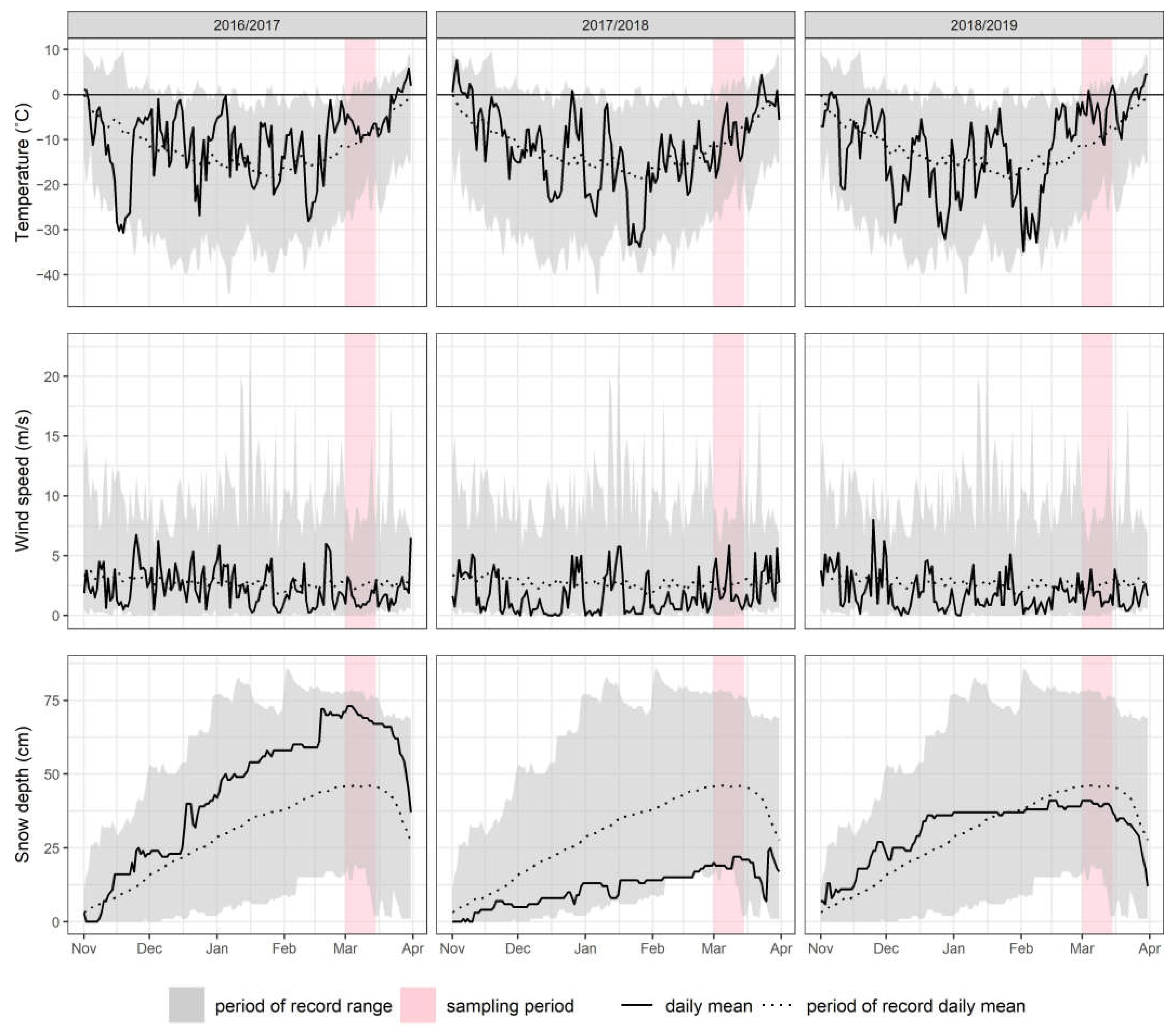
Figure 1. The Kasmala basin in the south of Western Siberia with sampling locations and land cover composition. NP—northern part, CP—central part, SP—southern part.
Forests 14 00160 g001
Figure 2. Barnaul weather station air temperature, wind speed, snow depth for the studied winter seasons as well as the station period of record (1966–2020).
Forests 14 00160 g002
Figure 3. Temporal variability of the isotopic composition (δ2H and δ18O) of bulk snowpack over the basin parts (NP, CP, SP) with results of Kruskal–Wallis tests within sampling years. Violin and Tukey outlier box plots show the median value (horizontal line within the box), the 1st and 3rd quartile (ends of the box), minimum/maximum values (whiskers) and distribution.
Forests 14 00160 g003
Figure 4. δ2H vs. δ18O plot over the basin parts (NP, CP, SP) and sampling years, including their regression lines (blue), global meteoric water line (gray), and snow depth gradient.
Forests 14 00160 g004
Figure 5. D-excess values over the basin parts (NP, CP, SP) and sampling years. Individual samples are shown using dots. Tukey outlier box plots show the median value (horizontal line within the box), the 1st and 3rd quartile (ends of the box), and the minimum/maximum values (whiskers).
Forests 14 00160 g005
Figure 6. Partial residuals of each predictor for the sampling years selected by the stepwise multiple regression. The dashed lines represent linear relationships.
Forests 14 00160 g006
Figure 7. Relationship of the d-excess and snow depth, SWE over the sampling years and basin parts (NP, CP, SP).
Forests 14 00160 g007
Table 1. Winter summary statistics with standard deviations at Barnaul weather station calculated from daily data [37].
Winter SeasonMean Temperature (°C)Mean Wind Speed (m/s)Peak Snow Depth (cm)
2016/2017−10.5 ± 7.82.3 ± 1.573 ± 22
2017/2018−11.9 ± 8.81.7 ± 1.625 ± 6
2018/2019−11.8 ± 9.41.9 ± 1.441 ± 10
Period of record (1966–2020) mean−11.5 ± 4.72.7 ± 0.330 ± 13
Table 2. Means and standard deviations of the bulk snowpacks SWE, depth, and isotopic composition, averaged over 2017–2019 and northern (NP), central (CP), and southern (SP) parts.
Sampling YearBasin PartDepth (cm)SWE (mm)δ18O (‰)δ2H (‰)d-Excess (‰)
2017NP71.4 ± 22.1196.6 ± 80.6−19.8 ± 0.7−151.2 ± 5.57.3 ± 1.7
CP69.5 ± 13.6169.7 ± 28.6−20.3 ± 0.5−156.7 ± 3.15.8 ± 1.9
SP80.4 ± 17.3212.2 ± 49.4−20.2 ± 0.6−154.6 ± 4.07.2 ± 1.9
2018NP27.8 ± 11.559.8 ± 40.9−19.5 ± 1.3−148.3 ± 9.37.4 ± 2.3
CP27.8 ± 8.941.6 ± 12.3−20.1 ± 1−154.9 ± 6.35.6 ± 2.4
SP36.8 ± 1067.1 ± 19.9−20 ± 1.1−152.6 ± 7.37.6 ± 2.2
2019NP44.1 ± 8.7103.6 ± 21.4−19.4 ± 0.8−148.1 ± 5.67.3 ± 1.0
CP40.8 ± 1091.7 ± 46.7−19.7 ± 0.7−151.9 ± 4.75.6 ± 1.6
SP56.6 ± 11.1108.7 ± 29−19.7 ± 0.8−150.6 ± 5.77 ± 1.8
Table 3. Kruskal–Wallis test results for snow isotopic composition (δ18O, δ2H, d-excess) among land cover types, basin parts, and sampling years.
FactorsDfH-Valuep-Value
δ18OSampling year214.00<0.001
Basin part29.740.008
Land cover27.130.029
δ2HSampling year215.54<0.001
Basin part218.2<0.001
Land cover215.79<0.001
d-excessSampling year23.080.21
Basin part 223.03<0.001
Land cover219.38<0.001
Table 4. Adjusted R2, slopes, and intercepts for computed regression equations describing H2 vs. land cover and topography predictors relationships (ns = predictor variable not selected).
Variables201720182019
Snow Depthns−0.608 ***−0.224 *
SWEnsnsns
TRI−0.445 ***ns−0.358 ***
General Curvaturensnsns
Forest rationsnsns
Slopensnsns
Aspect (Cos)−0.196 *nsns
Intercept0.0190.0250.013
R2a0.239 ***0.325 ***0.164 **
* p < 0.1; ** p < 0.05; *** p < 0.01.
Table 5. Adjusted R2, slopes and intercepts for computed regression equations describing d-excess vs. snow depth and SWE relationships (ns = predictor variable not selected).
Sampling YearEstimateSnow DepthSWE
2017Slopens0.3803 ***
Interceptns1.313 × 10−16
R2ans0.13 ***
Observations6060
2018Slope0.3124 **0.2509 *
Intercept−4.238 × 10⁻¹⁶−3.239 × 10⁻¹⁶
R2a0.08 **0.05 *
Observations6060
2019Slope0.4891 ***0.3737***
Intercept2.908 × 10−163.214 × 10⁻¹⁶
R2a0.23 ***0.13 ***
Observations6060
* p < 0.1; ** p < 0.05; *** p < 0.01.
Disclaimer/Publisher’s Note: The statements, opinions and data contained in all publications are solely those of the individual author(s) and contributor(s) and not of MDPI and/or the editor(s). MDPI and/or the editor(s) disclaim responsibility for any injury to people or property resulting from any ideas, methods, instructions or products referred to in the content.

