Article

Effect of Provenance and Environmental Factors on Tree Growth and Tree Water Status of Norway Spruce

by
Adriana Leštianska
1,*,
Peter Fleischer, Jr.
1,2,3,
Katarína Merganičová
4,5,
Peter Fleischer, Sr.
1,
Paulína Nalevanková
1 and
Katarína Střelcová
1
1
Faculty of Forestry, Technical University in Zvolen, T.G. Masaryka 24, 96001 Zvolen, Slovakia
2
Department of Plant Ecophysiology, Institute of Forest Ecology, Slovak Academy of Sciences, Štúrova 2, 96053 Zvolen, Slovakia
3
Administration of Tatra National Park, Tatranska Lomnica, 05960 Vysoke Tatry, Slovakia
4
Faculty of Forestry and Wood Sciences, Czech University of Life Sciences Prague, Kamýcká 129, Suchdol, 16500 Praha, Czech Republic
5
Department of Biodiversity of Ecosystems and Landscape, Slovak Academy of Sciences, Štefánikova 3, 81499 Bratislava, Slovakia
*
Author to whom correspondence should be addressed.
Forests 2023, 14(1), 156; https://doi.org/10.3390/f14010156
Submission received: 30 November 2022 / Revised: 27 December 2022 / Accepted: 12 January 2023 / Published: 14 January 2023

Abstract

:
Changes in temperature regime, and a higher frequency of extreme weather conditions due to global warming are considered great risks for forest stands worldwide because of their negative impact on tree growth and vitality. We examined tree growth and water balance of two provenances of Norway spruce growing in Arboretum Borová hora (350 m a.s.l., Zvolen, central Slovakia) that originated from climatologically cooler conditions. The research was performed during three meteorologically different years from 2017 to 2019. We evaluated the impact of climatic and soil factors on intra-species variability in radial stem growth and tree water status that were characterised by seasonal radial increment, stem water deficit and maximum daily shrinkage derived from the records of stem circumference changes obtained from band dendrometers installed on five mature trees of each provenance. The impact of environmental factors on the characteristics was evaluated using the univariate factor analysis and four machine learning models (random forest, support vector machine, gradient boosting machine and neural network). The responses to climatic conditions differed between the provenances. Seasonal radial increments of the provenance from cooler conditions were greater than those of the provenance originating from cooler and wetter conditions due to the long-term shortage of water the latter provenance had to cope with in the current environment, while the provenance from the cooler region was more sensitive to short-term changes in environmental conditions.

1. Introduction

Climatic factors belong to important factors determining species composition of ecosystems and driving ecophysiological processes that affect the overall functionality and stability of ecosystems. High temperatures coupled with changes in the water cycle are most frequent ecological limits of production potential of forest tree species that can worsen the health status and may cause their die-back [1,2]. Drought and drying-out of central European countries is one of the important bioclimatic elements, which is expected to increase in the future [3].
The need to adapt forest ecosystems to future climatic conditions by changing tree species composition is often in contrast to the lack of knowledge about the potential abilities of individual tree species and provenances to resist changed environmental conditions [4]. Provenance experiments represent a suitable tool to assess the adaptation potential of provenances under the conditions of climate change [5]. Due to the long-term adaptation to local conditions, the performance and vitality of populations remain related to ecological characteristics of the place of their origin, even after their transfer to a new environment [6]. Considering the natural climatic changes in the direction from west to east, the population of tree species originating from central and eastern Europe is becoming more prospective due to the higher resistance to drought and low temperatures [7,8].
Norway spruce (Picea abies L. Karst) belongs to the tree species with the greatest distribution range. It is a dominant tree species in the boreal forests covering Scandinavia up to the Ural Mts., as well as in mountainous areas of the temperate zone with low temperatures and high precipitation amounts [9,10]. During the last 200 years, Norway spruce, as economically the most important coniferous tree species in Europe, was frequently planted outside its natural distribution range [11] i.e., in warmer and drier areas, where currently it is under great pressure [12]. Due to the shallow root system, spruce is not well adapted to the environment outside its natural distribution range, particularly at sites with extreme climatic conditions [13,14], and its productivity is restricted by water availability [15]. The ongoing changes in precipitation events significantly manifested in the reduction of soil water and further increase the drought risk for spruce [16]. Many studies focused on spruce growth rate and performance at different elevations, latitudes or along gradients [17,18].
Climatic characteristics are important factors affecting stem radial growth and wood production. Changes in stem diameters are the results of formation of xylem tissues and tree water balance that causes stem swelling and shrinking depending on water uptake and outflow. From the point of daily changes in stem dimensions, the temporal development of transpiration and soil water content is important [19,20]. As presented by Zweifel et al. [21], sap flow transporting nutrients and water via xylem directly affect reversible changes in stem circumference, i.e., its swelling and shrinking. The amplitude of daily shrinking is a function of water loss from leaves and water absorption by roots. More detailed information about xylem and phloem formation can be found in e.g., Mäkinen et a. [22], Oberhuber et al. [23], Swidrak et al. [24].
Continual observations of stem radial changes during a year are useful for understanding tree reactions to short-term changes of environment. The reversible living cell dehydration–rehydration processes are related to depletion and replenishment of stem water stored in the inner bark tissues. These processes are detectable through high temporal resolution measurements of stem radius variations with dendrometers [25,26]. This approach has been increasingly used in plant physiology to analyse tree growth and water status [27,28]. Stem water deficit (ΔW) and maximum daily shrinkage (MDS) used in this study represent indirect measures of plant water status compared to direct methods, such as leaf water potential or relative water content. Continuous non-destructive measurements of radial stem changes allow us to have closer looks and a deeper understanding of tree water dynamics and growth without the need to perform a complicated sampling of foliage from tree crowns to determine water potential [27,28]. Continuous observations of stem radial changes provide us with the time series of tree water storage fluctuations at different temporal scales including daily changes due to water depletion and refilling of water storages [29,30] up to seasonal tree growth [31,32,33] and its relationship with changing environmental conditions [27,34,35].
In general, stem growth follows a seasonal development and is strongly affected by meteorological variables. Meteorological events fluctuate within and between years. Therefore, detailed analyses focusing on the relationship between the climate and seasonal tree growth are necessary to quantify potential tree growth reactions to changing climate. Seasonal tree growth development depends not only on climate, but also on tree species [20,24,36], tree social position [37], genetics [38], etc.
This study analysed tree growth reactions and tree water status of two Norway spruce provenances growing outside the production optimum with regard to climate of their original site and current site. Such an experiment allows the assessment of the importance of adaptation to the site of origin and acclimation to new conditions. The examined provenances have been growing under same conditions since their planting for several decades. Their seasonal growth was monitored with band dendrometers at high temporal resolution for several years. The measurement period covered contrasting climatic conditions including extremely dry and hot periods in the years 2018 and 2019 and relatively wet conditions in the year 2017. The study analysed intra-species seasonal dynamics of stem circumference changes and characteristics of stem water status: stem water deficit (ΔW) and maximum daily shrinkage (MDS) derived from band dendrometer records (hereafter as BDR) considering selected factors of environment. Several authors [21,27,28] pointed out that ΔW and MDS can be interpreted as a direct measure of drought stress in trees.
The study was conducted to establish a better understanding of the effect of changed conditions on stem circumference changes and sensitivity of the tree species and provenances to weather conditions. The primary question of our research was to examine if the spruce trees of two provenances follow different physiological and growth patterns that reflect their adaptation potential and to reveal which provenance tolerates changed conditions more. We hypothesised that the provenance originating from the site characterised with the lower mean temperature and the same precipitation total as the current site would show enhanced regulatory mechanisms that help to improve its response capacity and the adaptive potential to stress factors. We hypothesised that the provenance that originated from the site at the higher elevation with the lower mean temperature and the higher precipitation total than the current site would be more sensitive to warmer and drier conditions.

2. Materials and Methods

2.1. Study Area and Plant Material

The experiment was performed in Arboretum Borová hora located in Zvolen valley, central Slovakia (48°35’ N, 19°07’ E, elevation approximately 350 m a.s.l.). Arboretum Borová hora is a specific facility aimed at growing native tree species, as well as species of different geographical origins due to their intra-species and geographical variability with the aim to preserve a gene pool of the Carpathian dendroflora ex situ [39]. The research site is situated in a south-west facing slope with a mild 5%–10% inclination. The soil type is cambisol (https://geo.enviroportal.sk/atlassr, accessed on 20 September 2021). The study area is characterised by temperate central European climate and belongs to a warm and a slightly warm region with cold winters. The long-term mean annual air temperature is 7.9 °C, and annual precipitation total is 651 mm. The long-term (1961–1990) average temperature during a growing season (April–October) is 13.6 °C and the respective precipitation total is 422 mm (derived from long-term measurements at a nearby meteorological station of Sliač, 313 m a.s.l., managed by the Slovak Hydrometeorological Institute) (Table 1).
Two research plots, each representing a single provenance, were selected at sites with similar environmental conditions. The climatological conditions of the study area are warmer and drier than original natural habitats of the Slovak provenance labelled as CW_PV (PV stand for a provenance, while CW indicates its origin from cooler and wetter conditions) and warmer than original natural habitats of the Russian one labelled as C_PV (the provenance from cooler conditions) (Table 1). The Slovak provenance originated from the Podtatranská valley characterised with the long-term mean annual temperature of 5.3 °C and precipitation total of 833 mm. Mean temperature and precipitation total during a growing season (April–October) is approximately 10.7 °C and 603 mm, respectively. Russian provenance originated from Archangeľskaja and Volgogradskaja regions where the long-term mean annual temperature is approximately 2.0 °C and precipitation total is 587 mm. Mean temperature and precipitation total during a growing season (April–October) is approximately 9.5 °C and 404 mm, respectively (Table 1). The description of climatic conditions of provenance origins was derived from CRUTEM4 datasets [40] and Panoply software.
At each plot, we chose five vital adult trees (49 and 53 years old) of similar dimensions. The diameters at breast height of the CW_PV and C_PV were 25.3 ± 3.5 cm and 27.3 ± 1.4 cm, respectively, and their heights were 23.0 ± 2.4 m and 24.7 ± 0.6 m, respectively.

2.2. Environmental Data

During the study period, meteorological data were recorded with an automatic meteorological station (EMS Brno, Brno, Czech Republic) installed at an open grass area situated 80–150 m from the research plots. The meteorological station recorded global radiation (GR, W.m−2), air temperature (AT, °C), relative air humidity (RH, %), wind speed (WS, m·s−1) and precipitation (P, mm) with automatic sensors every 10 min. The sensors for global radiation (EMS11), air temperature and relative air humidity (EMS33) were placed at a height of 2 m above the low-cut grass. Precipitation was measured using a rain gauge Model MetOne370 (Met One Instruments, Inc., Grants Pass, OR, USA) located at a height of 1 m above ground. Automatically measured data were stored in the datalogger in 10-min intervals. Daily and monthly values of mean air temperature, mean relative air humidity, precipitation totals and global radiation sums were derived from recorded meteorological measurements. Mean vapour pressure deficit in the air (VPD, Pa) was calculated as follows
V P D = e s   e a
where es (Pa) is the saturated vapour pressure at a given air temperature and ea (Pa) is the vapour pressure of the free-flowing air.
Potential evapotranspiration (PET, mm) as a variable representing theoretical atmospheric evaporative demands unaffected by soil water deficit was calculated according to the Penman equation [41]
P E T = + γ R n + γ + γ 6.43 1 + 0.536 W S   V P D λ
where ∆ is the slope of the saturation vapour pressure curve (kPa·K−1), Rn is the net radiation (W·m−2) estimated as 77% of the global incoming solar radiation [42] and WS is the wind speed measured at 2 m height. The psychometric constant (γ) was set to 66 Pa·K−1 and the latent heat of vaporisation (λ) was 2.45 MJ·kg−1 [42].
From the point of vegetation, it is insufficient to evaluate climatic conditions only using the summary values of precipitation or temperature. Moisture conditions are frequently described using the climatic water balance (CWB) characterised as a difference between precipitation and potential evapotranspiration. Water availability was assessed with the climatic water balance (CWB) defined as a difference between the precipitation (P) and potential evapotranspiration (PET during a specific period (Equation (3)). Negative values of CWB indicate water deficit, while positive values indicate water surplus.
C W B = P P E T
Daily CWB values were cumulated to obtain the cumulative water balance during a growing season.
Soil water potential (SWP, bar) was measured under forest canopy at 15, 30 and 50 cm soil depths using MicroLog SP3 (EMS Brno Ltd., Brno, Czech Republic) with gypsum blocks (Delmhorst Inc., Towaco, NJ, USA). SWP values varied between 0 and −1.5 MPa (the lowest measurable limit of the equipment). Measuring intervals were set to 20 min. For this study we used daily mean SWP values calculated from all depths separately for each plot.

2.3. Band Dendrometer Records (BDR)

Stem circumference changes of each of 10 sample trees (five trees per provenance) were monitored using high temporal resolution automatic band dendrometers (model DRL 26, EMS Brno, Brno, Czech Republic, accuracy ±1 µm) installed at a height of 2.5 m. To ensure a close contact of dendrometer bands with tree stems and to reduce the influence of hygroscopic swelling and shrinkage of the bark, the outermost part of the bark (periderm) was removed prior to the installation of dendrometers. Circumference measurements were recorded in 20-min intervals from April 2017 to October 2019.

2.4. Data Analysis and Statistical Evaluation

Basic data processing was performed with Mini32 software produced by EMS Brno (Brno, Czech Republic) compatible with all used equipment.
To quantify tree water status, we applied two indicators derived from BDR. The first indicator is stem water deficit (∆W in mm) defined by Zweifel et al. [21] and Ehrenberger et al. [43]. It defines the actual tree state in comparison to a fully hydrated state. It was calculated as a difference between the actual BDR value and the growth line value, which represents a tree state under fully hydrated conditions (i.e., when ∆W = 0) [27]. The growth line was derived from BDR using a moving maximum of the current and previous dendrometer readings. Hence, negative values of ∆W indicate the lack of water, i.e., drought stress.
The second indicator is maximum daily shrinkage (MDS in mm) defined as the difference between daily maximum and minimum stem circumferences (BDR). Hence, it quantifies the daily cycle of water uptake at night and water loss from elastic cambial and phloem tissues during a day [26]. Both indicators (∆W and MDS) were calculated with ‘DendrometeR’ R package [44].
Daily stem radial increment (I) was calculated as a difference between the actual daily maximum and the previous maximum in BDR. Following the concept of Zweifel et al. [45], irreversible stem growth (I) is restricted to the period within a day, when the stem shrinkage does not occur. Reversible stem shrinkage is in contrast with the irreversible stem increment, which we call growth here (I) (following the methodologies of Downes et al. [31] and Deslauries et al. [32]).
The relationships of daily environmental variables (precipitation (P), relative air humidity (RH), vapour pressure deficit (VPD), minimum, maximum and mean air temperature (ATmin, ATmax, ATavg), potential evapotranspiration (PET), climatic water balance (CWB), cumulative water balance (CWBcum), soil water potential (SWP)) with daily parameters extracted from BDR (∆W, MDS) within the analysed period of the year (April–October) were quantified with the Spearman rank-correlation coefficients in the statistical software Statistica® 12 (Statsoft, Tulsa, OK, USA).
Besides the classical correlation analysis, we used machine learning methods (ML) to examine the relations between tree water status characteristics (ΔW, MDS) and environmental conditions. We decided to use these methods to capture non-linear and complex relationships and analyse the suitability of selected models for predictions. ML methods use the ability of computer algorithms to make unique decisions on their own, based on the existing data and experience [46]. Machine learning techniques are widely used for prediction and classification purposes. The advantage of machine learning techniques is their robustness against correlation structures (multicollinearity) and the presence of outliers. In our study we used the following four machine learning techniques:
  • Random forest (RF) is a decision tree nonparametric algorithm for classification or regression [47]. The algorithm selects a random number of samples from training datasets, what is called a bootstrap aggregation [48]. Afterwards, the randomly chosen samples are used to develop a decision tree based on the most important variables. For each prediction, multiple decisions trees are constructed, and the average value is outputted.
  • Gradient boosting machine (GBM) is also based on decision trees. The main difference to RF is that the random forest uses averaging, while the gradient boosting provides additive (ensamble) modelling [49]. Moreover, the random forest combines results at the end of the process, while the gradient boosting combines the results along the way.
  • Support vector machines (SVM) are used both in classification and regression. In support vector regression, the space that is required to fit the data is referred to as a hyperplane [50]. A hyperplane is a subspace with the number of dimensions equal to that of the original space minus one. The best fit is the hyperplane that contains the maximum number of points within threshold values. This separates SVM from other regression models which minimise errors between real and predicted values. The hyperplane is determined using a kernel, which is a set of mathematical functions that takes data as input and transforms it into the required form.
  • Neural networks (NN), also known as artificial neural networks (ANNs), are composed at least of three layers: input, output layers and one or more hidden layers. Each neuron has a specific weight and a threshold value and is connected to other neurons. If the output of a neuron exceeds the threshold value, the neuron is activated and sends the signal (data) to the next layer of the network [51]. Deep neural network (DNN) refers to the situation when more than one hidden layer is applied. The deeper the DNN, the more complex patterns the network can learn [52].
To enhance the stability of the four mentioned ML models and to avoid overfitting, all models were ten-fold cross-validated. To reach the optimal performance of models, specific hyperparameters were tuned, or grid searched for random forest [53]. Support vector machine models were constructed and tuned in R environment using the caret package [54]. NN and GBM were compiled and tuned in Python environment. After hyperparameter tuning, created models were passed to Dalex package [55] which operates both in Python and R. More details about the hyperparameter grid search, model selection and tuning of models can be found in the Appendix A.
We randomly split the data into training (66%) and validation (33%) subsets prior to the model development. The models were trained on the training dataset and their performance was assessed using the validation subset. The same split was applied also to datasets which were used for hyperparameter tuning. The results of ML models were interpreted on the basis of (1) partial dependence plots (PDP) and (2) variable importance (VI). Partial dependence plots show marginal effects of a single characteristic on the predicted outcome of used machine learning models. VI was calculated by means of permutations using the root mean square loss function [56] in Dalex environment.
We used 11 variables (day of the year (DOY), i.e., the sequential day number starting from 1 on 1st January, and daily values of environmental factors of all study periods of the years 2017–2019 together: global radiation (GR), average air temperature (ATavg), minimum air temperature (ATmin), maximum air temperature (ATmax), relative air humidity (RH), precipitation (P), vapour pressure deficit (VPD), potential evapotranspiration (PET), soil water potential (SWP), climatic water balance (CWB) and cumulative water balance (CWBcum)) in each model and analysed their influence on ΔW and MDS.

3. Results

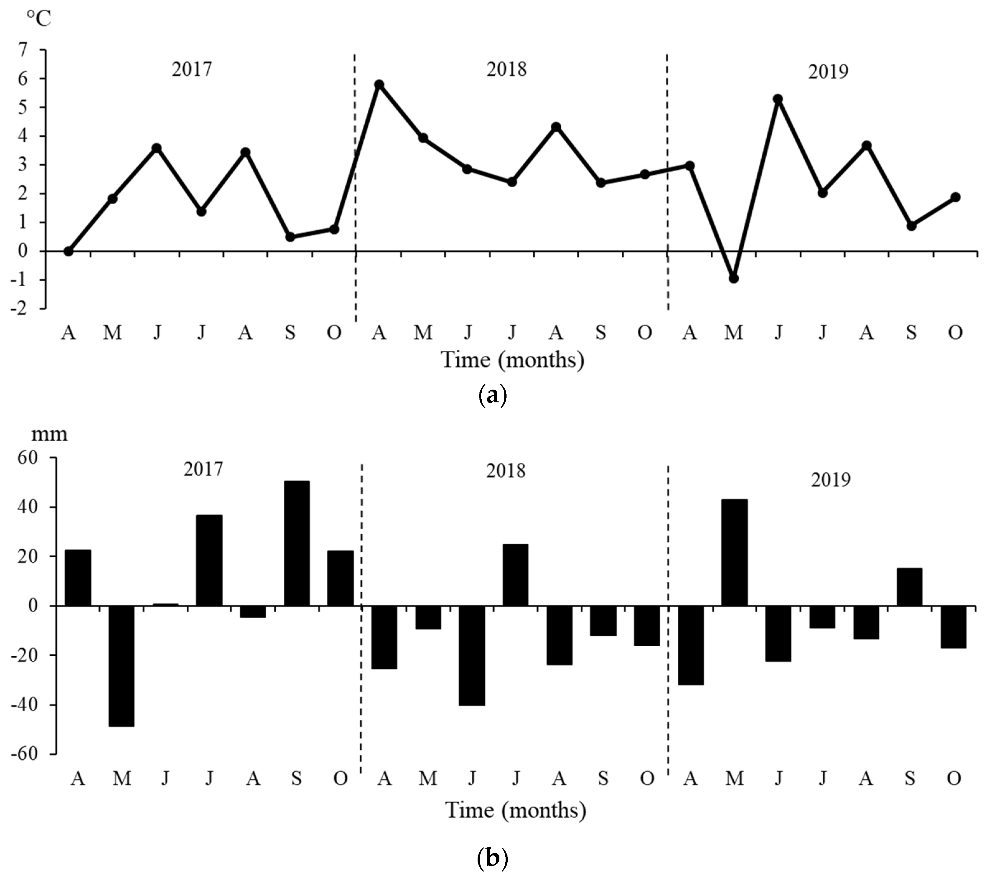
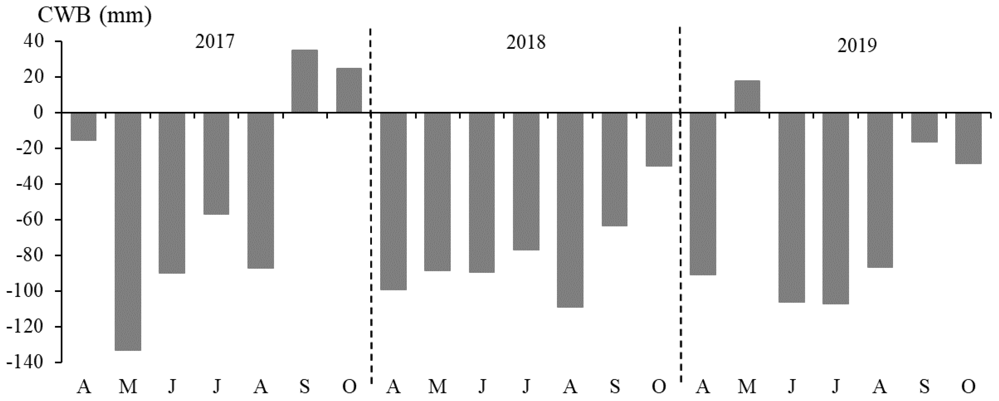
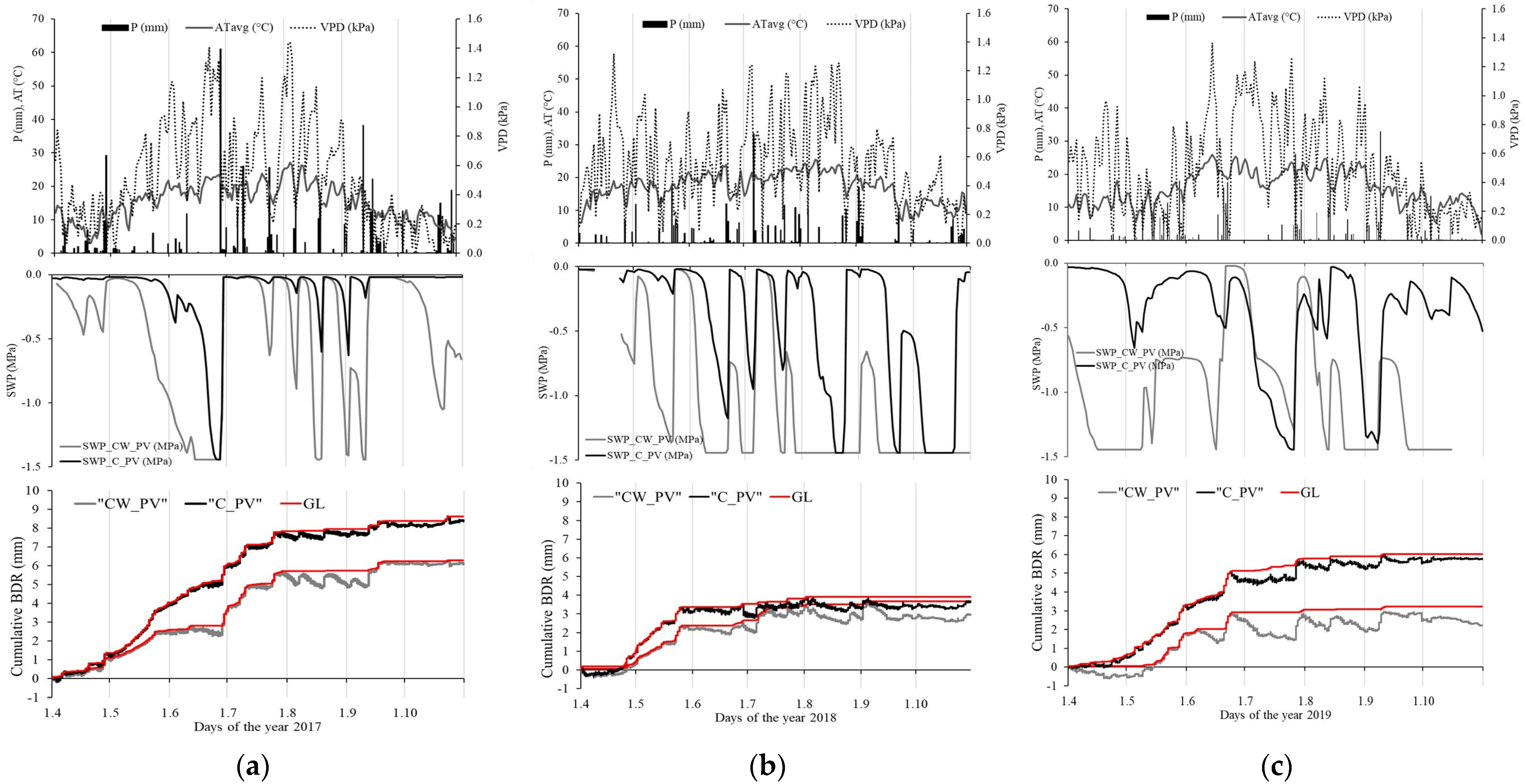
3.1. Environmental Variables during the Growing Seasons of the Years 2017–2019

The monitored period (2017–2019) was interesting because it included climatically contrasting years, during which several climatic and meteorological extremes occurred (Table 2, Figure 1 and Figure 2). The mean air temperature of every season exceeded the long-term mean value (1961–1990). The highest mean air temperature during the growing season observed in the year 2018 (17 °C) was by 3.4 °C above the long-term average (1961–1990). Air temperature in all individual months in the growing seasons (April–October) of the years 2017 to 2019 except May 2019 was above average (Figure 1a). Precipitation events were irregularly distributed in time (Figure 1b, Figure 3a), which affected the values of SWP (Figure 3b). The lowest precipitation total in the growing season (320 mm) was observed in the year 2018, when we also recorded the highest values of VPD, and the lowest values of PET and CWB (Table 2). Monthly precipitation totals in all monitored months except July of the year 2018 were below their long-term averages. In contrast, the value of seasonal precipitation total exceeding the long-term average was observed in the year 2017. Monthly precipitation totals in the year 2017 were greater than the long-term averages in most months, excluding May and August (Figure 1b). In the year 2019, we observed lower precipitation total than the long-term average (1961–1990). The seasonal mean air temperature in the year 2019 was higher by 2.2 °C than the long-term average, but lower compared to that in 2018 (Table 2).
Positive values of CWB indicate sufficient precipitation amount, while its negative values indicate the lack of precipitation and drought risk. During the monitored period from 2017 to 2019, we recorded only three months with moisture surplus (September and October 2017, May 2019) (Figure 2). In general, CWB indicated insufficient moisture conditions especially in the year 2018 followed by the year 2019. The highest but still a negative CWBcum value was recorded in the year 2017 (Table 2).

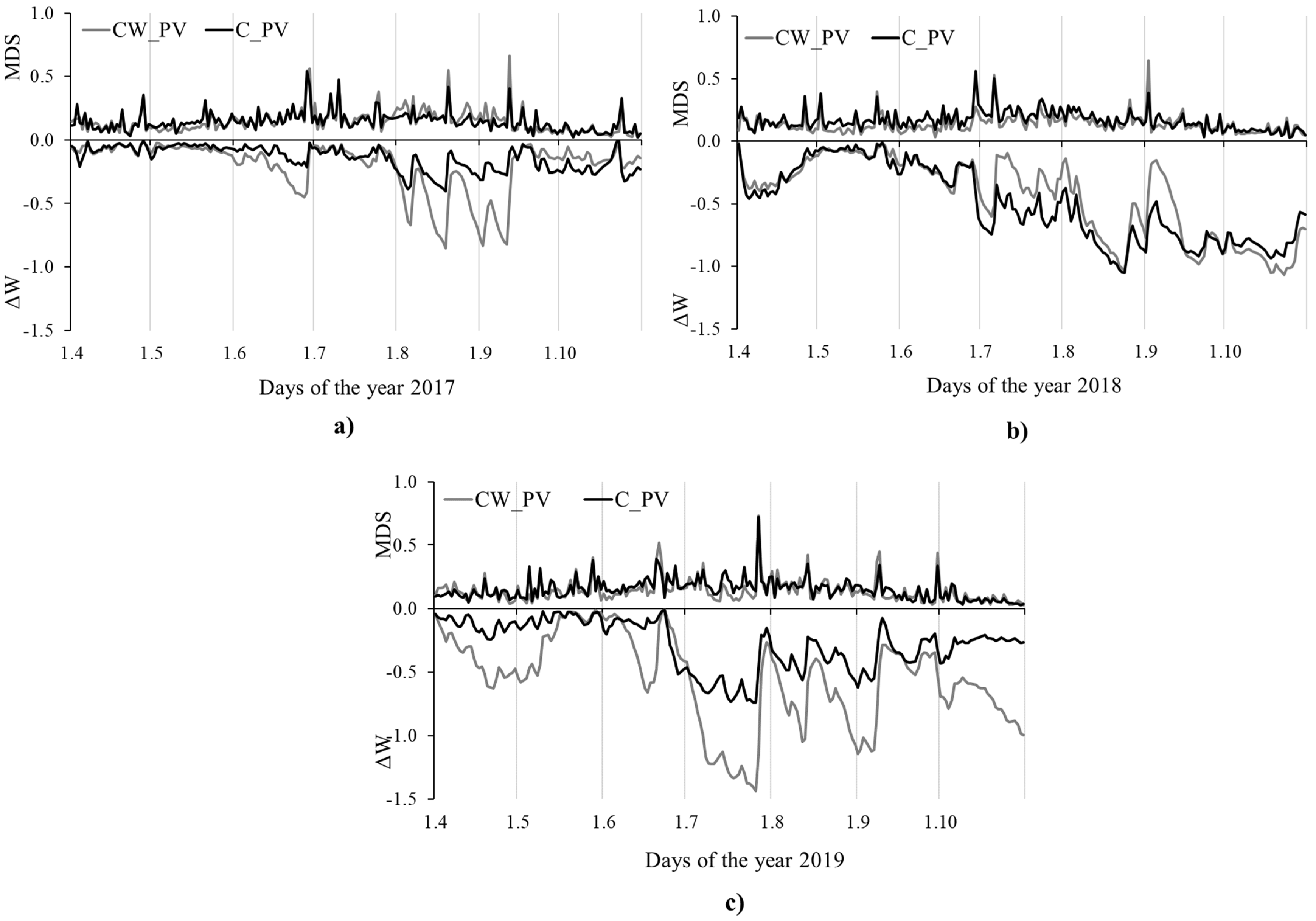
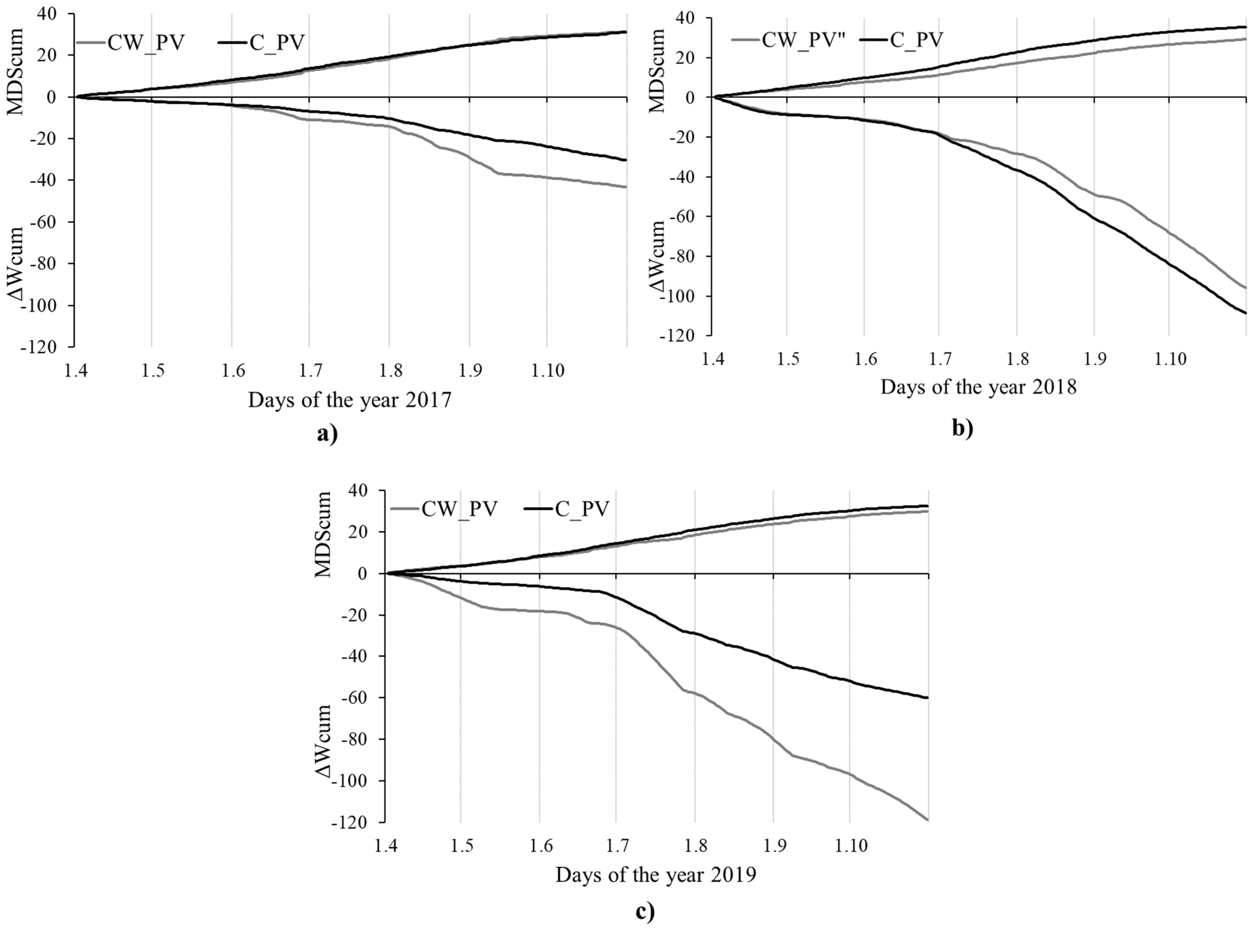
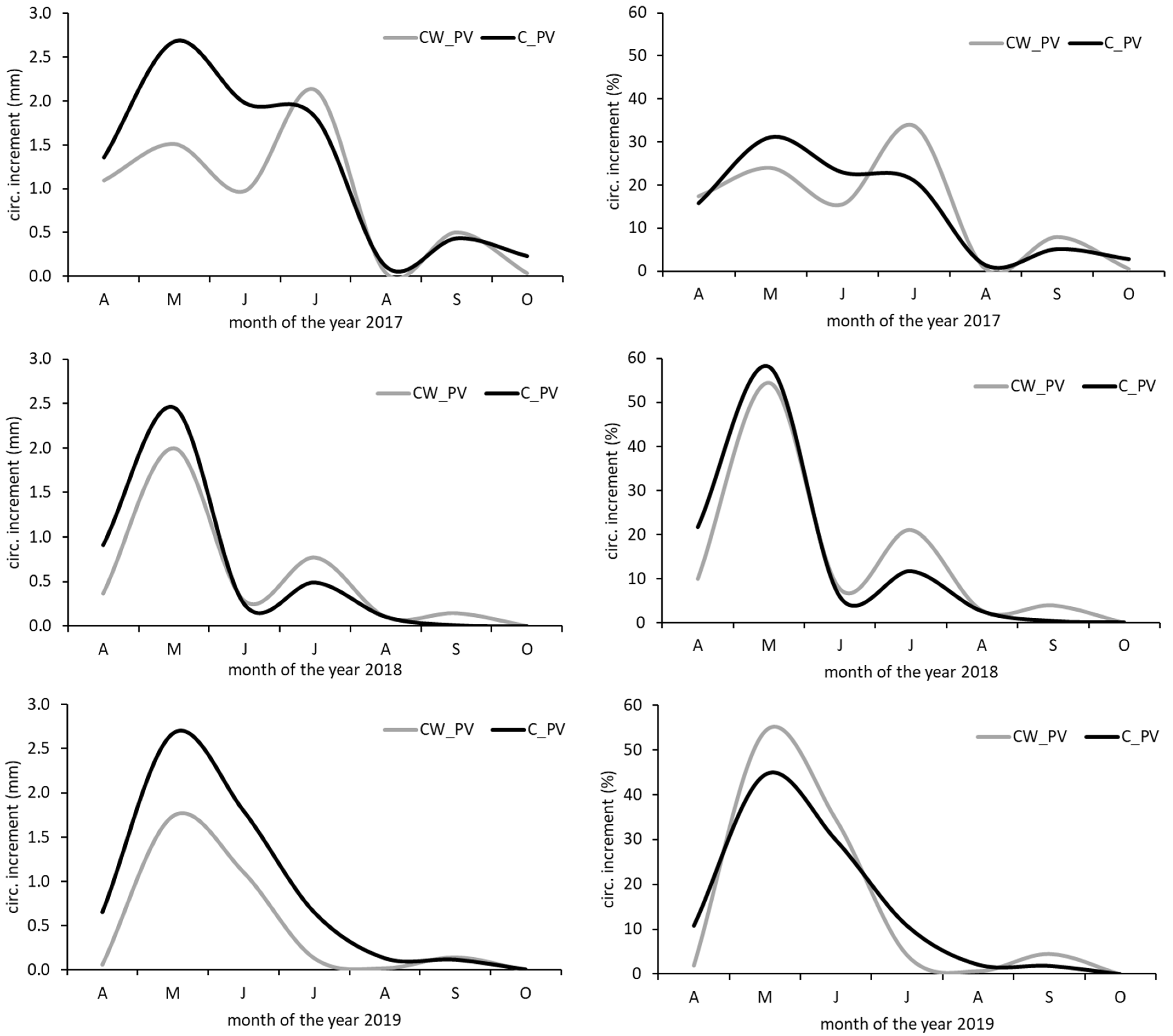
3.2. Stem Radius Changes and Stem Water Status

Band dendrometer records (BDR) and seasonal increments differed between provenances and years (Figure 3a–c, Table 3). Trees of the C_PV had a more intense growth with smaller fluctuations than the CW_PV (Figure 3a–c). However, there was an interannual synchronous course of BDR, ΔW and MDS between provenances (Figure 3 and Figure 4). In all monitored years, seasonal radial increments of the C_PV were greater than those of the CW_PV (Figure 3a–c, Table 3). The highest seasonal radial increments of both provenances were recorded in the year 2017 (Figure 3a, Table 3). In contrast, the radial increment in the year 2018 was only a half of the increments achieved in the year 2017, while we also revealed the smallest difference between the provenances (Figure 3b, Table 3). The greatest proportion of radial increments was usually formed at the beginning of the growing season, mainly in May. In the year 2017, we observed more intense radial growth also in June and July (Figure A1). On the contrary, at the beginning and the end of June 2019 we recorded substantial stem shrinkages of both provenances due to the low precipitations and highly above normal air temperatures. Growth stagnation of both provenances was observed from the beginning of August onwards in all seasons. In the year 2018, radial growth started to stagnate at the end of May because of the above-normal air temperature and low precipitation total (Figure 3b).
Derived ΔW and MDS of both provenances showed synchronous fluctuations in all monitored seasons (Figure 4). The increase in negative values of ΔW indicates the increase of water shortage in storage tissues. During the monitored seasons, stem water deficit gradually decreased (Figure 5). This trend was occasionally disrupted by precipitation events, after which stem water deficit reached values close to zero (Figure 3 and Figure 4). When we examined total cumulative changes in stem water content in individual seasons, we found that the cumulative ΔW of the CW_PV was the lowest in the year 2019 (−118.87 ± 25.64 mm) and the highest in the year 2017 (−95.66 ± 35.05 mm). The C_PV had the lowest and the highest values of the cumulative ΔW in the years 2018 (−107.80 ± 63.18 mm) and 2017 (−30.37 ± 13.30 mm), respectively (Table 3, Figure 5). Cumulative values of stem water deficit for the whole seasons were greater for C_PV in comparison to CW_PV in the years 2017 and 2019, while in the year 2018 the values of ΔWcum of C_PV were lower than those of CW_PV from the beginning of July until the end of the growing season (Figure 5b, Table 3). In June and July 2018, air temperature substantially dropped and was followed by higher precipitation in July (Figure 1). Later, air temperature increased while precipitation was low (Figure 1 and Figure 3), ΔW of C_PV provenance decreased more than of CW_PV (Figure 4b and Figure 5b). The greatest difference in ΔWcum between provenances was recorded during the whole growing season in 2019 (Figure 4c and Figure 5c, Table 3).
The seasonal cumulative shrinkage (MDScum) of provenances in individual years increased in the following order: 2018, 2019, 2017 in the case of the CW_PV, and 2017, 2019, 2018 in the case of C_PV (Figure 5, Table 3). In drier years of 2018 and 2019, the C_PV provenance had higher values of MDScum, while in the year 2017, which was more favourable from the point of water, higher MDScum was observed for the CW_PV. The greatest difference in MDScum between provenances was recorded in the year 2018 (Figure 4b and Figure 5b).

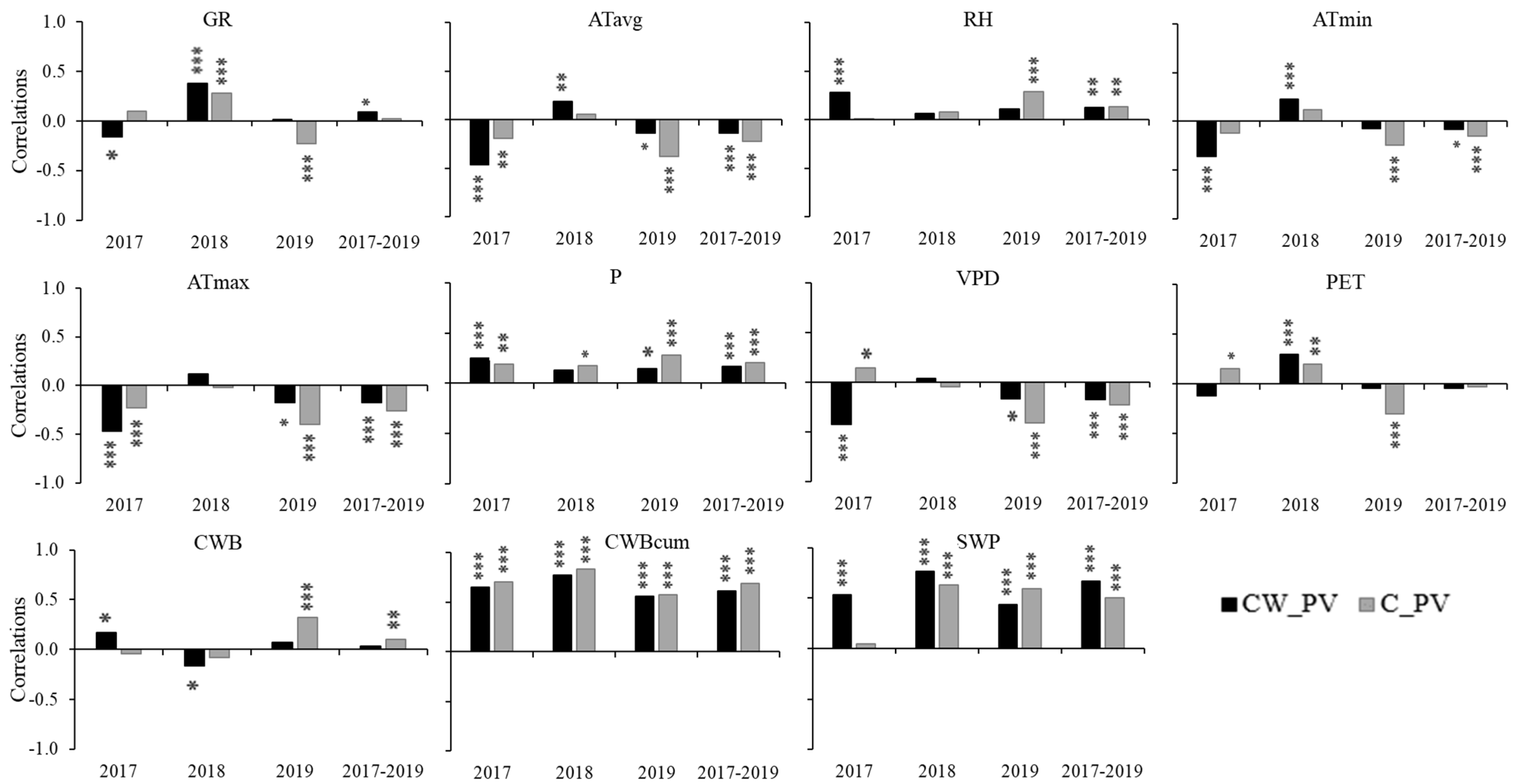
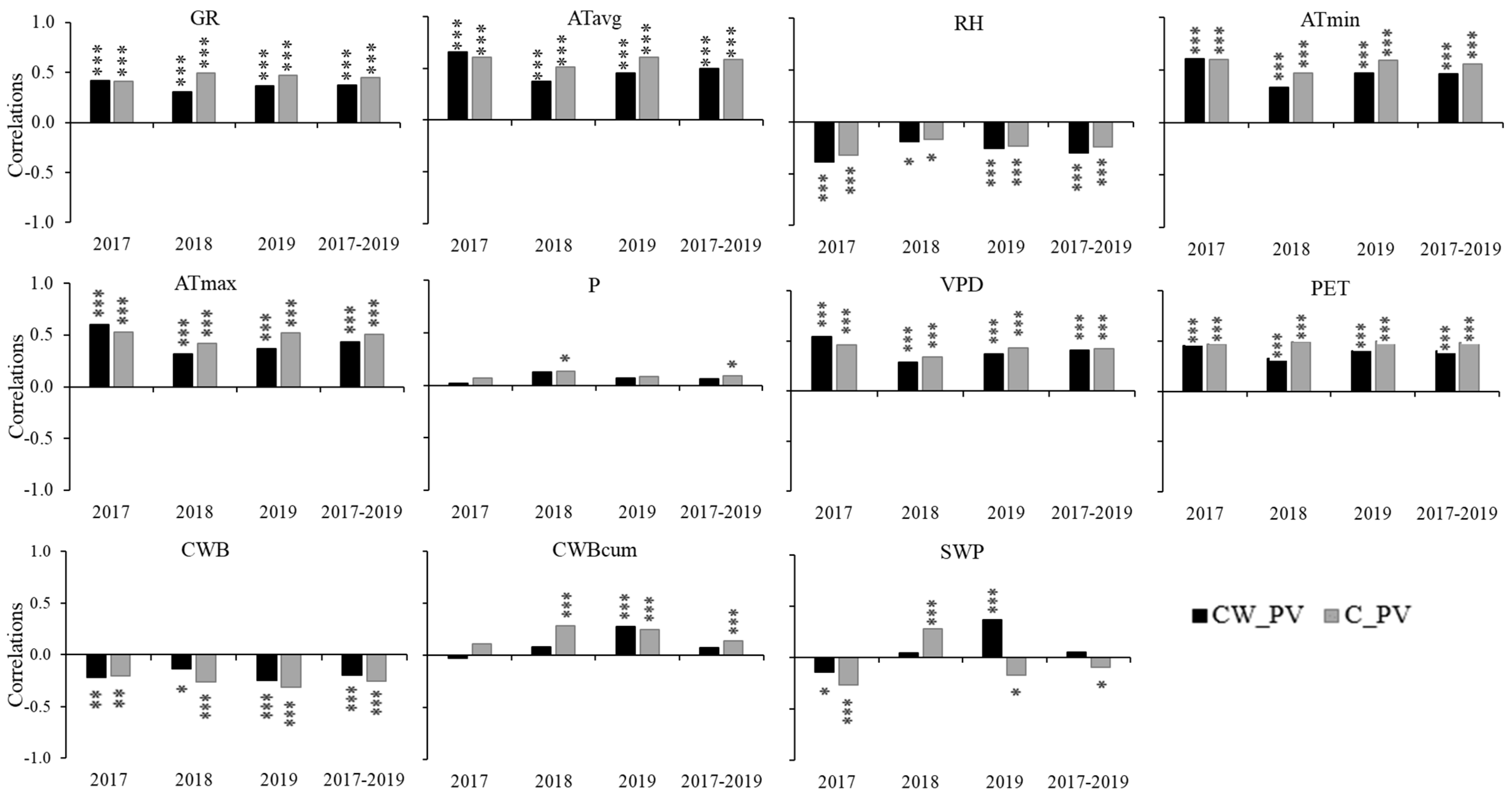
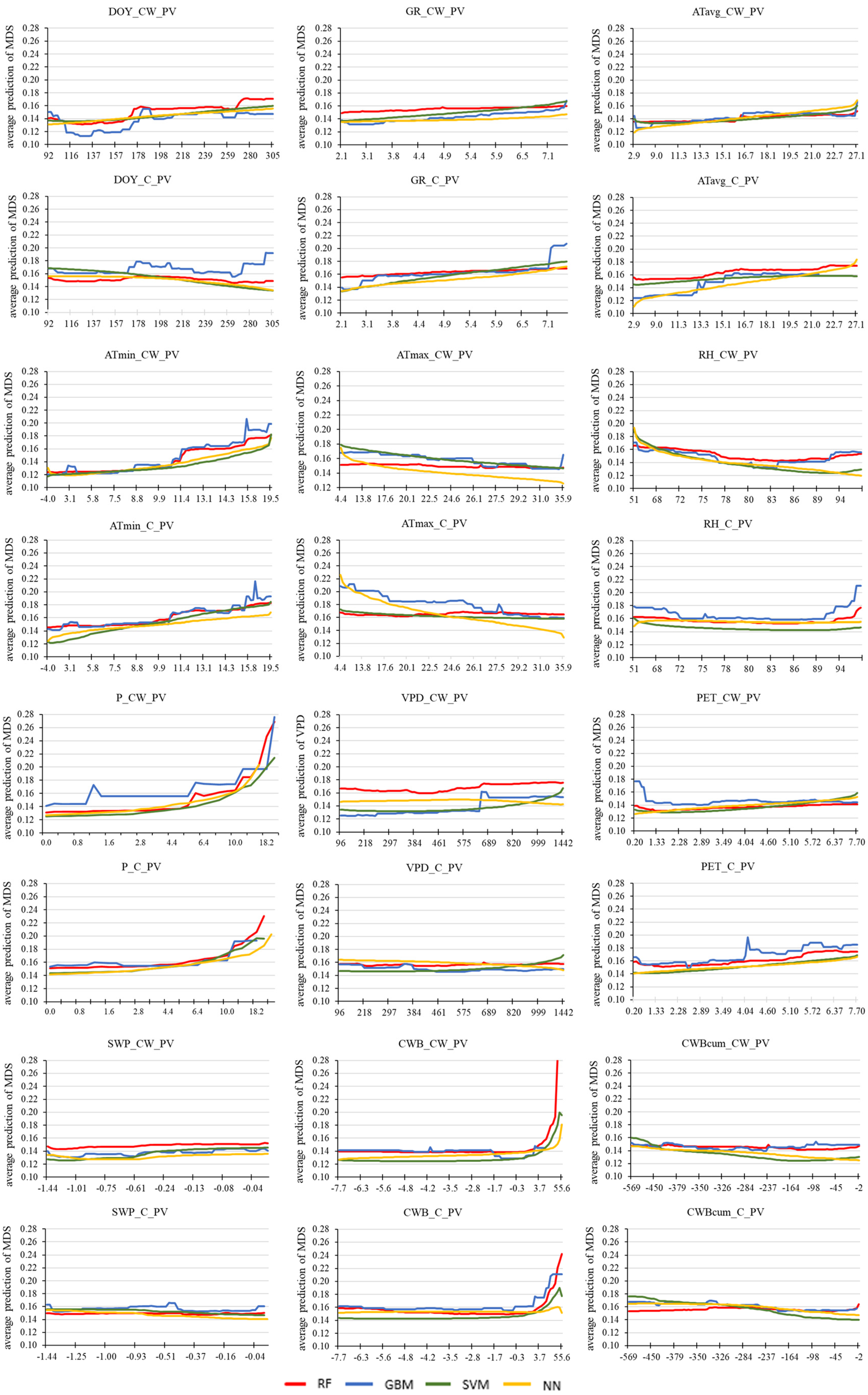
3.3. Influence of Environmental Variables on Growth and Tree Water Status

We analysed the impact of monitored environmental factors on daily changes of tree water status (stem water deficit and maximum daily shrinkage) during individual growing seasons (1 April–30 October) as well as in the whole monitored period 2017–2019 (Figure 6 and Figure 7) with Spearman correlation coefficients. The analysis revealed negative correlations of stem water deficit of both provenances to ATavg, ATmax, VPD and PET in the years 2017 and 2019, but not in the year 2018. High and significant values of correlation coefficients were revealed between ΔW and CWBcum as well as SWP for both provenances in almost all periods (Figure 6). The results of a single factorial correlation analysis showed that during the whole period 2017–2019, stem water deficit of either provenance was not significantly affected by GR or PET. ATmin was significant only for the C_PV.
The daily values of GR, ATavg, ATmin, ATmax, VPD and PET significantly positively correlated with daily values of MDS regardless of the provenance, while higher values of correlation coefficients were observed for the C_PV. Significant negative correlations of MDS were observed with RH and CWB in all seasons. The relationships with RH were usually tighter for the CW_PV. The correlations between daily precipitation and MDS were low and significant only for the C_PV in the year 2018 and the whole period 2017–2019. The correlation between SWP and MDS changed in time. In the year 2017, the correlations of both provenances were negative and significant. On the contrary, in the year 2018 the correlations between SWP and MDS were positive for both provenances. In the year 2019 we observed a significant positive correlation for the CW_PV provenance, and an insignificant negative correlation for the C_PV. When analysing the whole monitored period, SWP values were not significantly correlated with MDS of either of the provenances (Figure 7).

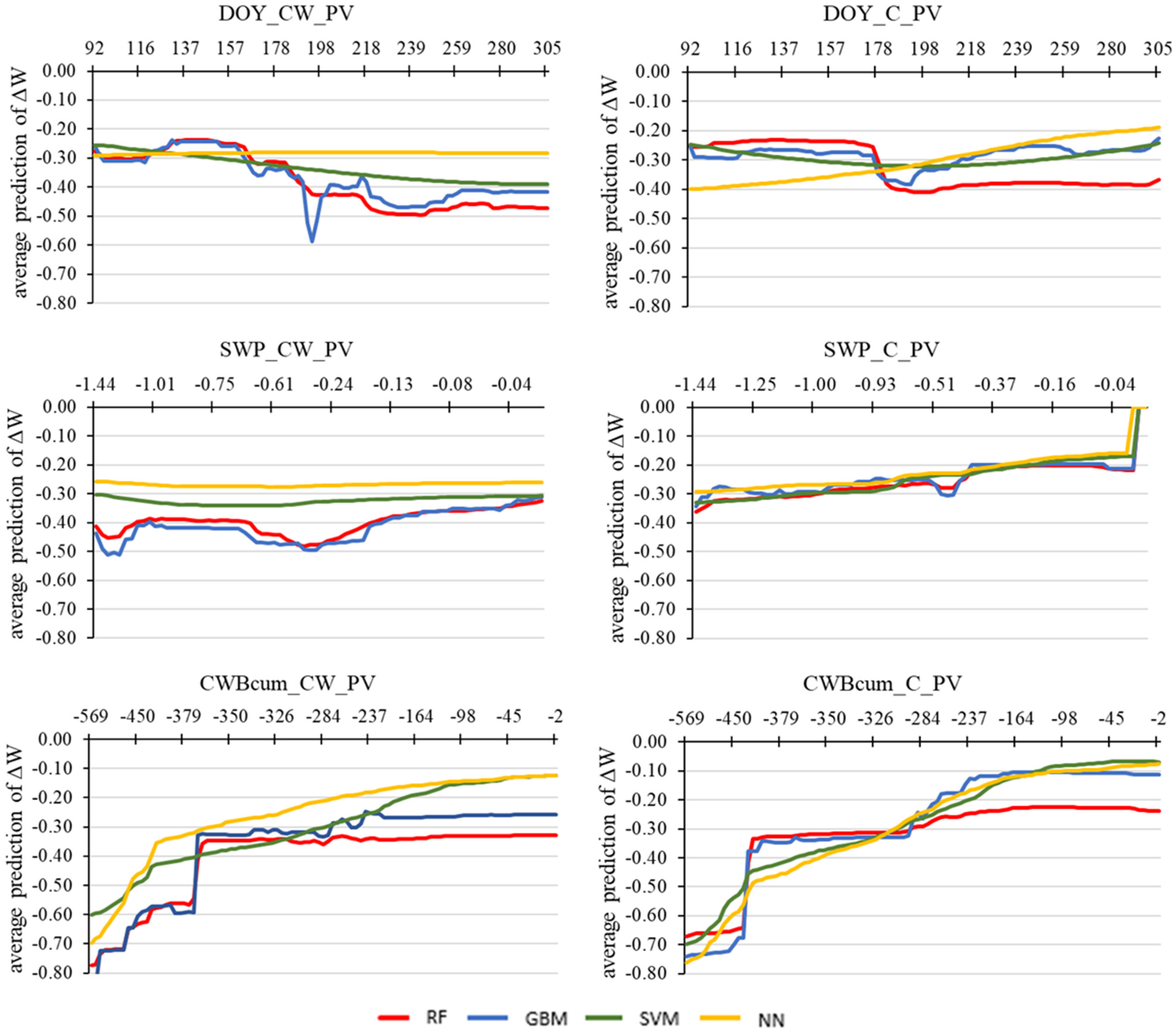
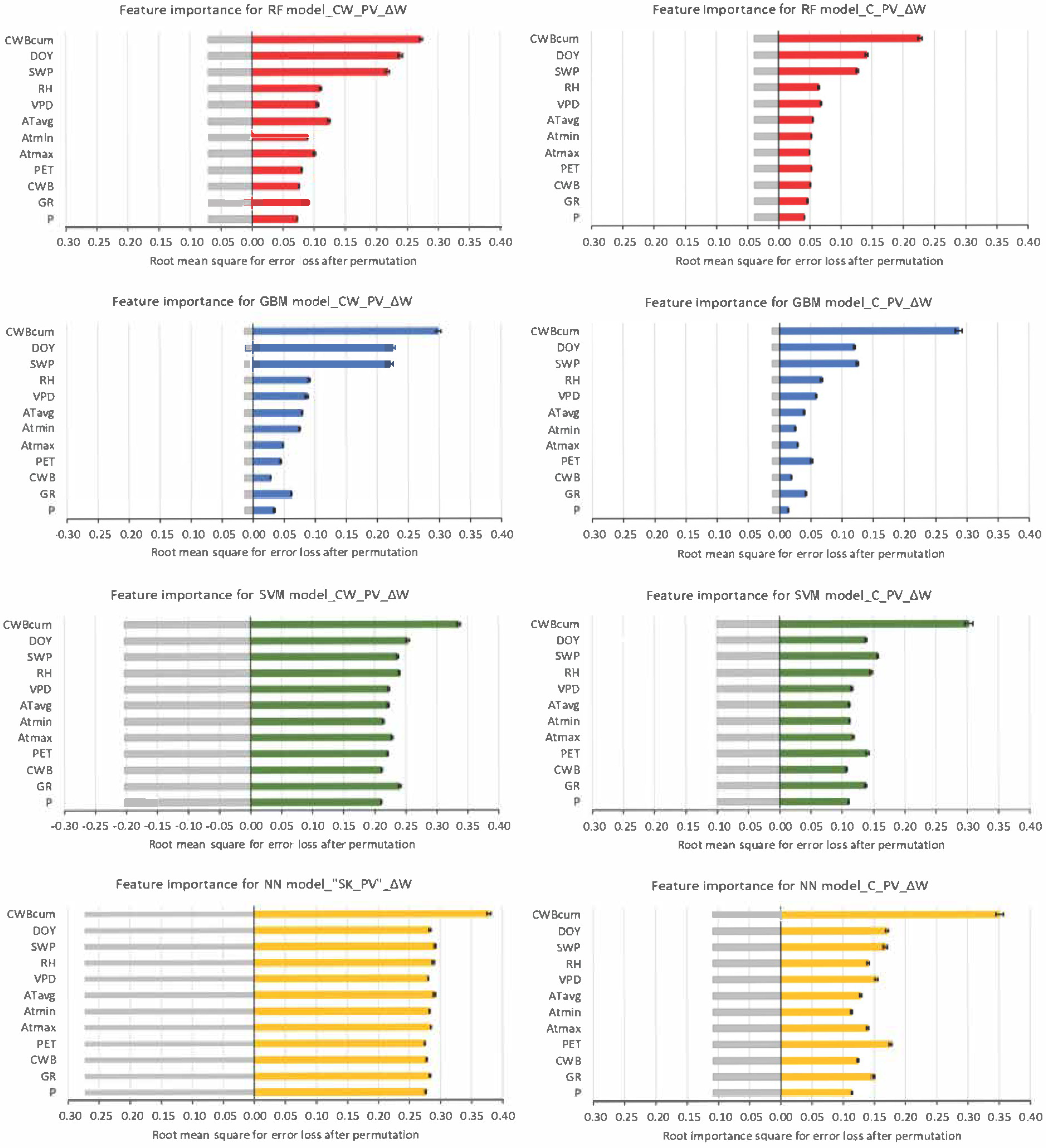
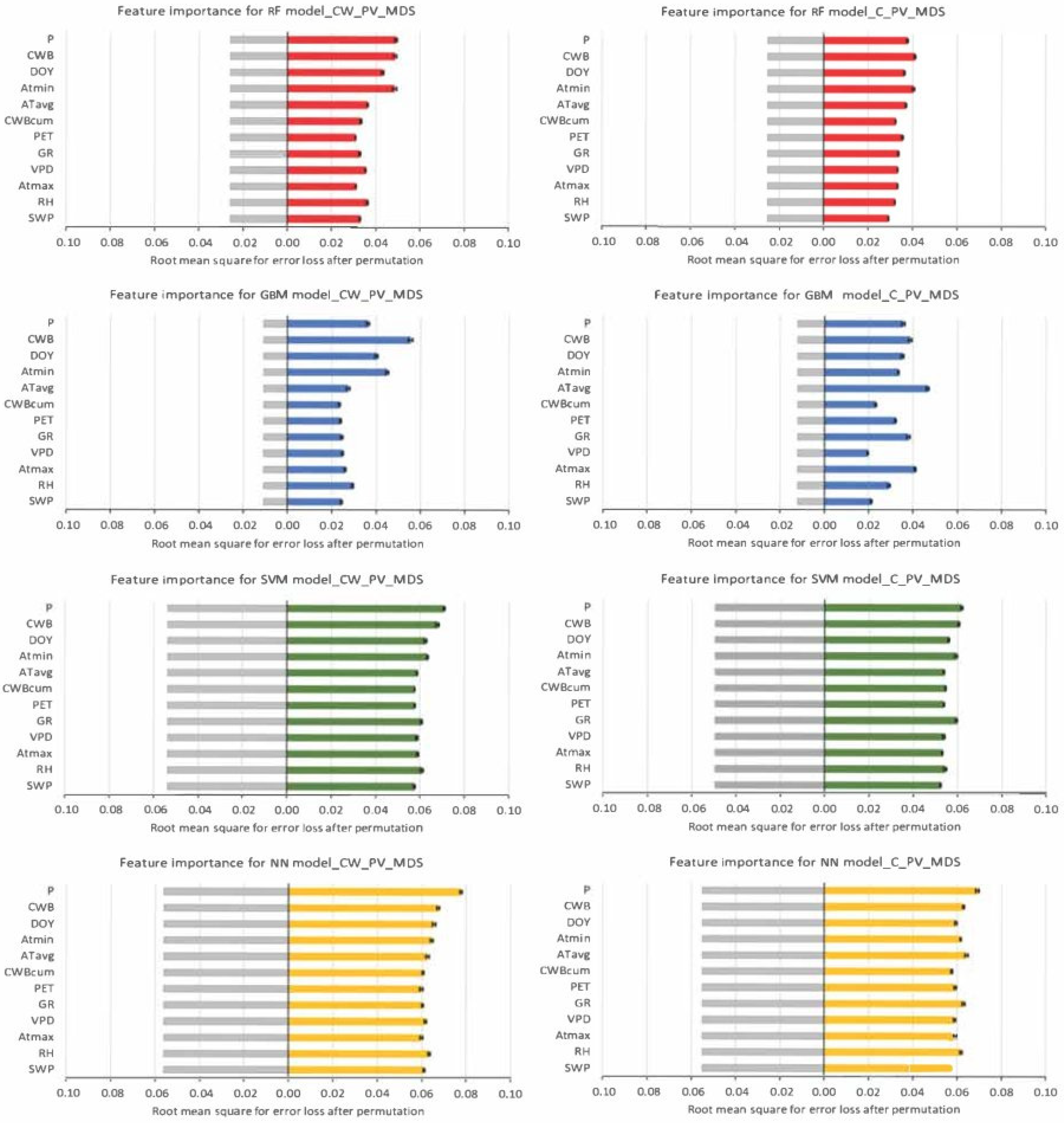
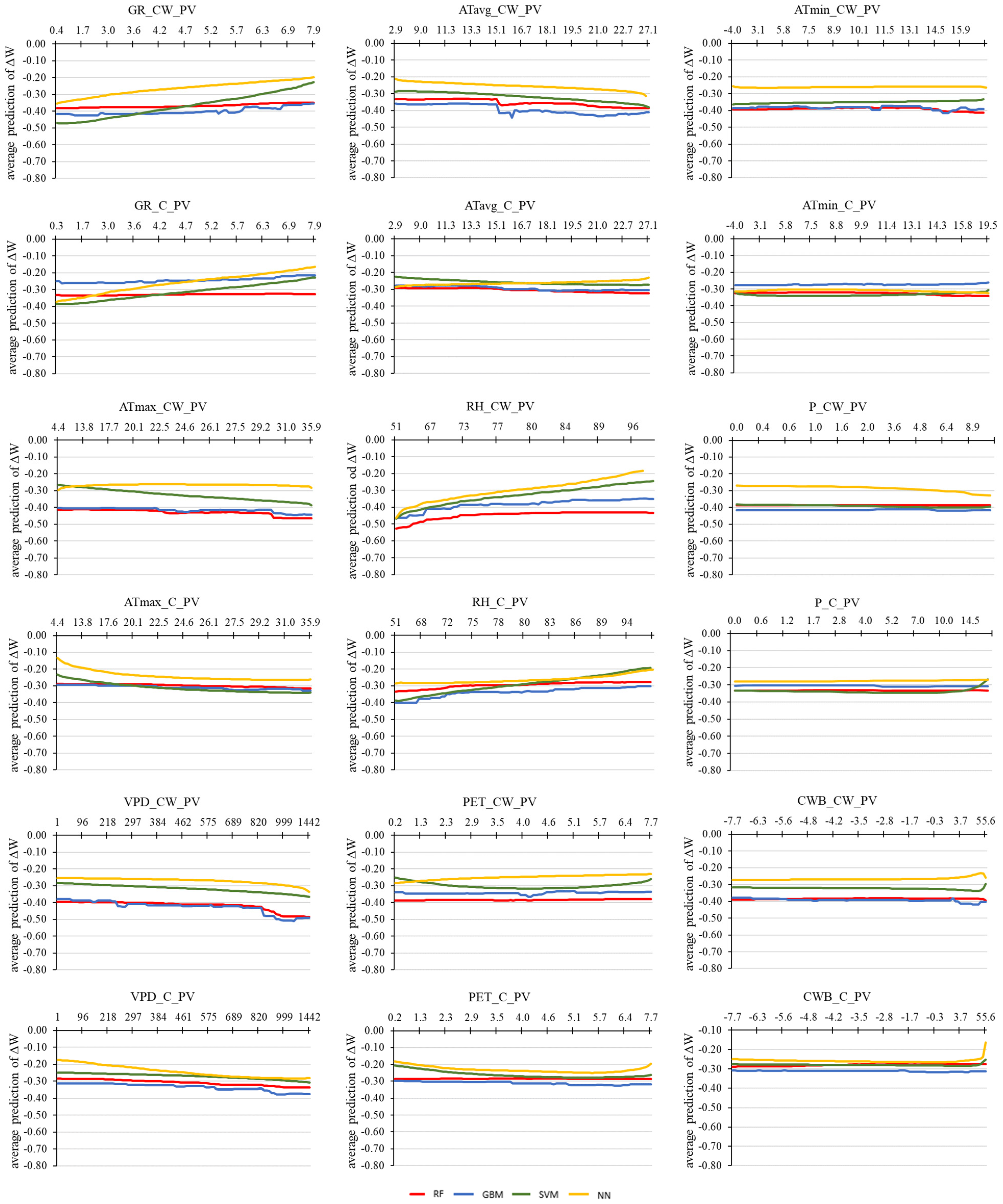
3.4. Machine Learning Techniques for Detecting the Influence of Environmental Factors on the Predicted Tree Water Status Characteristics

The ability of the four derived machine learning models to predict ΔW or MDS based on selected environmental characteristics was good as they explained more than 50% of the variation in stem water deficit (Table 4). Based on the partial dependence plots and performance of ML models we divided predictors of ΔW into strong (presented in Figure 8) and weak (Figure A2). Under strong predictors we understand most important predictors in each model that have a nonlinear effect on ΔW and had high variable importance values. The predictors SWP, DOY and CWBcum were strongest in RF and GBM models (Figure 9). In SVM and NN models, CWBcum was the only strong predictor with a higher variable importance value. Other predictors did not have a pronounced effect on the model performance (Figure 9). The CW_PV provenance had greater values of the residual error after permutation in comparison to C_PV (Figure 9).
Partial dependence plots of all models derived for both provenances follow the same course (Figure 8). The intra-annual changes of ΔW were provenance- and model-specific (Figure 8). The SVM and NN models usually showed a more smoothed performance of ΔW along the range of predictors than the GBM and RF models, which captured subtler changes. Moreover, the models revealed different intra-annual trends between the provenances. While ΔW of CW_PV had an overall slightly decreasing trend in the growing season across three derived models, the temporal changes of ΔW of C_PV were smaller and the trends were inconsistent between the models (Figure 8). In the case of SWP, all models predict a continuous decrease in ΔW with the increasing lack of soil water, while the reduction of CW_PV was less distinct than for C_PV. (Figure 8). Similarly, the decrease in CWBcum resulted in a continuous decrease of ΔW irrespective of the provenance, while CWBcum lower than 360 mm or 430 mm cause a more substantial reduction of ΔW for CW_PV and C_PV, respectively (Figure 8).
The other predictors (GR, VPD, AT (avg, max, min), P, PET, CWB, VPD) showed ‘flatter’ courses of ΔW along their ranges indicating lower sensitivity of ΔW to the varying predictor state. We can also observe an increasing discrepancy in offsets between tight (GBM, RF) and loose (SVM, NN) models (Figure A2).
When evaluating MDS we could not identify key factors influencing MDS behaviour based on the results from the machine learning models (Figure 10 and Figure 11). All predictors had relatively uniform effects on reducing root mean square error after permutation (Figure 11). The most important variables in all models for C_PV were DOY, P and GR, while CWBcum was important in the GBM and ATavg in the RF models. The MDS of the CW_PV was most affected by CWB followed by DOY, ATmin and P.
The models of intra-annual temporal development revealed that in the case of CW_PV its values slightly increased over time, while three out of four derived models showed the opposite trend for C_PV (Figure 10).
All models predict an increase of MDS with the increasing ATmin, AT avg, GR and P regardless of the provenance, while the trend with ATmax was the opposite. Both provenances showed synchronous, more less flat courses indicating lesser sensitivity of MDS values to VPD, PET, CWBcum and SWP. The relationship of MDS with precipitation and CWB was found to follow an exponential pattern. Hence, their impact on MDS substantially increased if their values exceeded 10 mm or 3.5mm, respectively (Figure 10).

4. Discussion

Norway spruce is known to be a plastic coniferous tree species growing in different environmental conditions [57,58]. Since its plasticity has its limits, the impact of climate change is unsure [59]. The assisted transfer of genetic material suitable for future environmental conditions may reduce the negative impact of climate change [60]. The research of tree growth response to different environmental conditions provides us with the information on the mutual effect of the genotype and the environment, adaptability of tree species and their provenances, and enables us to predict the impacts of the climate change [61,62,63]. The ongoing climate change, especially the temperature increase during the second half of the 20th century cause drought stress in spruce stand [64]. Stands growing outside their natural distribution region are especially sensitive to these impacts. Previous studies of spruce growth response to increasing temperatures presented contradictory results including a higher productivity particularly at higher elevations [1,65,66] and a decreasing trend in growth especially at lower altitudes [67,68,69]. Some research indicated that spruce can profit from warmer but not drier conditions [65,70]. [71] found that spruce trees at higher elevations were growing more slowly than those at lower elevations. Experiments showed that the phenology of provenances remains unchanged even after they are transferred from sub-alpine locations to lower elevations with more favourable growing conditions [71]. However, general trends found for a continental scale do not have to apply to all populations and local environmental factors need to be accounted for [72,73]. Based on model simulations, [74] predicted that an increase of air temperature by 1 °C would cause an increase in the average annual increment of spruce at the age of 100 years by 5.9%, while the increase by 3 °C could result in its reduction by 8.9%.
Several dendroecological studies (e.g., [4,67,75,76] confirmed a greater susceptibility of Norway spruce to drought in comparison with other tree species. It is particularly limited by drought in summer, most probably due to its shallow root system [77,78] and the majority of fine root located in the upper soil layers [79].
To better understand Norway spruce sensitivity to drought stress, hydraulic and physiological mechanisms of tree species reaction to environmental conditions need to be examined. The World Meteorological Organisation (WMO) reported that the period 2015–2020 as well as the whole last decade 2011–2020 in Europe was historically the warmest period over the last 140 years. The climatic data measured at our site revealed that the air temperature during the growing season was the highest in the year 2018 (by 3.4 °C more than the long-term value), while the precipitation total was the lowest and below the long-term normal (1961–1990) (Figure 1, Table 2). In the year 2018, central Europe experienced one of the most severe and longest summer heat and drought periods. As presented by [80], drought events in the year 2018 were climatically more extreme and had a greater impact on the European forest ecosystems than the drought in the year 2003. Due to the extreme drought, many species experienced high tree mortality in the whole Europe [80].
The changes in climatic factors during the growing season cause changes in the growing abilities of tree species, which are directly linked to biomass accumulation [21]. In addition, tree growth is also driven by its size, age, competition, and site conditions. Previous studies showed that in some regions, competition is the driving factors, while the climate impact is secondary [37,81]. This trend was particularly evident for dominant species [82], while in plantation forests, the relative influence of competition decreased but that of climate increased [83]. In our case, research plots resemble plantations since trees are of the same age and were planted at regular distances at the same time. Hence, we focused on selected climatic and soil conditions, and disregarded other growth conditions.
The spruce provenance originating from cooler conditions (C_PV) had a better growing performance than the provenance from cooler and wetter conditions (CW_PV) in all investigated growing seasons (Figure 3, Table 3) indicating that the reduction of the available water resulted in less growth. The cumulative radial increment of CW_PV during the whole period 2017–2019 represented 70% of C_PV increment (Table 3). The substantial increase in air temperature by 5 °C in comparison to the site of the origin coupled with the sufficient amount of precipitation in the year 2017 (by 100 mm, i.e., 20%) resulted in the greatest radial increment of C_PV during the investigated period indicating that the water is the driving factor. The response of CW_PV was more complex, since the lowest radial increment (although not significantly different from other years) was observed in the year 2019, which was not the least favourable one in the three years from the point of climatic conditions.
The smallest difference in the annual radial increment between the provenances was recorded in the year 2018 (Figure 3, Table 3), which was characterised by highly above average values of air temperature and low precipitation totals during the whole growing season. In that year, the radial increments of C_PV and CW_PV represented only 22% and 28% of the total increment for the analysed period, respectively (Figure 3, Table 3).
Norway spruce is very sensitive to soil water supply (see e.g., [37,67,84]), which was also observed in our results. Greater values of MDS and lower values of ΔW were found when SWP was low (Figure 3, Figure 4 and Figure 5). Decreasing stem water deficit indicates the reduction of water potential in stem tissues, which can result in stem shrinkage lasting up to several days or weeks [20]. In the years 2017 and 2019, the lack of water was more pronounced for the CW_PV provenance, while in the year 2018 the situation was the opposite due to climatically more extreme conditions compared to 2017 and 2019. In the year 2018, the precipitation total below the long-term precipitation of the C_PV original location (Table 1 and Table 2) coupled with the highest recorded mean air temperature in the observed period caused a greater reduction of radial increment and Wcum than in the case of CW_PV (Figure 3, Figure 4 and Figure 5, Table 3). We assume that this result is caused due to the fact that CW_PV had to cope with more extreme conditions (Table 1 and Table 2) at the current site throughout its whole growth, and that is why it reacted to a lesser extent than C_PV. Spearman correlations for the year 2018 revealed opposite relationships of ΔW with several environmental factors than in the other two years (Figure 6). These results reflect the changes in the tree reaction to the lack of water availability. After reaching a threshold of stem shrinkage, trees were not able to reduce their radial dimensions further. The positive correlations of stem water deficit with GR, AT and PET in the year 2018 (Figure 6) may result from the isohydric behaviour of spruce [85], and the reduction of stomatal conductance in the early stages of soil drought, which affected the overall growth performance (Figure 3b). Norway spruce has a more risk hydraulic strategy than e.g., white fir [86,87]. If the hydraulic system is damaged, water transport can be reduced for a longer time despite the sufficient amount of available water [88]. The protracted lower post-drought growth of spruce may indicate that a tree was damaged during a drought event, which has subsequent longer-term legacy impacts (cf. [62,80]).
The driving impact of water availability on ΔW was confirmed by the highest values of Spearman correlation coefficients of stem water deficit with CWBcum and SWP (Figure 6), as well as by models derived by machine learning methods (Figure 8 and Figure 9). CWBcum combines the impact of multiple variables (precipitation, air temperature, radiation, air humidity), and is a cumulative characteristic similarly as ΔW, which explains the greatest influence of CWBcum on ΔW (Figure 8 and Figure 9).
Several authors (e.g., [21,89,90]) found that ΔW is closely related to drought stress, and is determined by a combination of atmospheric and soil conditions, which was confirmed also by our results. The values of SWP at CW_PV site were usually lower than at CV_PV site (Figure 3), which can explain the higher sensitivity of ΔW to SWP (Figure 6) and a smaller radial increment of CW_PV (Table 3). Models also showed a significant impact of SWP on ΔW, while the response of CW_PV to SWP was greater (Figure 8). These observations coincide with the previous research that showed a close relationship between a diameter of coniferous tree species and soil water availability or evaporation demands [21,91].
Three models based on artificial intelligence (RF, GBM and SVM) revealed a significant impact of DOY on ΔW. The relationship between DOY and ΔW reveals the seasonal development of ΔW. DOY can also be considered as a proxy of tree phenology. PDP shows the impact of individual predictors on the dependent variable, e.g., ΔW, while the effect of all other independent variables is excluded. The NN model was not sensitive enough to capture the impact of DOY (Figure 8). The seasonal development of ΔW indicated that C_PV had a higher ability to cope with the water deficit in the season (Figure 8).
In the wetter year 2017 (Figure 1 and Figure 3a, Table 2), we recorded the lowest differences in cumulative MDS between provenances compared to all analysed years. Although SWP at C_PV site was almost during the whole examined period greater than at CW_PV (Figure 3), in drier years of 2018 and 2019 smaller cumulative values of MDS were observed for CW_PV (Figure 5, Table), which may indicate that C_PV was more sensitive to atmospheric factors. This assumption was confirmed by the correlation analysis, since the coefficients of MDS to climatic variables were greater for C_PV (Figure 7). Considering the fact that the maximum daily shrinkage quantifies stem shrinking for one day [26], it is an indicator of real tree plasticity to current environmental conditions including atmosphere and soil [92,93]. Due to this, its relationship to independent characteristics is more balanced than in the case of ΔW, which was affected mainly by DOY, SWP, CWBcum (Figure 8, Figure 9, Figure 10 and Figure 11). Moreover, extreme values of MDS occurred more rarely than in the case of ΔW, which has a cumulative character. Periods of missing stem rehydration are represented in ΔW but not in MDS. The duration of reversible changes of stem diameters (contraction, expansion) depends mainly on the transpiration of the whole plant [25]. As presented by Giovanneli et al. [90], the increase in MDS is the first visible morpho-physiological signal of changes in tree water status. Greater MDS values indicate large gradients between water demand and supply [94], and/or days with open stomata and hence with high transpiration and assimilation. If water potential falls below a certain threshold [95], photosynthesis and structural growth [23,77] are substantially reduced. The accumulation of above-ground biomass is affected more [96], and photosynthetic activity is usually maintained at a lower level to ensure the survival of the whole organism. Isohydric species, such as Norway spruce, reduce their water consumption and growth already at an early stress phase by closing stomata, which reduces the risk from drought stress. Considering this knowledge, the lower radial increment of CW_PV than of C_PV indicates that trees of CW_PV close their stomata sooner to reduce their water demand due to the long-term insufficient water supply at the current site in comparison to the site of the provenance origin. On the other hand, C_PV originating from the site with the same precipitation amount is adapted to such conditions and thus, its radial growth was more intense. Considering the hypotheses about the sensitivity of investigated provenances that were planted under different environmental conditions, our results suggest that the temporal aspect needs to be accounted for. The provenance CW_PV originating from more extreme conditions had lower absolute radial increments in comparison to C_PV, but it was less sensitive to short-term changes of climatic conditions. To formulate a general conclusion, more detailed analyses including more provenances and/or longer time series covering more years are required.
In this paper we applied four machine learning models, which can be utilised for the prediction of daily drought indices: ΔW and MDS from environmental variables (Figure 8, Figure 9, Figure 10 and Figure 11). We must be aware that climatic predictors are highly correlated. The emerging multicollinearity is well handled by RF and GBM [97,98]. However, there is an emerging danger in overfitting the model when correlation structures between features in the training set do not generalise the unseen data. In general, this is not our case except for precipitation which is characterised by the random pattern of precipitation events. Nevertheless, precipitation had the lowest importance from predictors in the models for ΔW (Figure 9).
Neural networks do not suffer from multicollinearity, as the parameters are estimated using the backward propagation, which eliminates this problem. In the models derived based on the support vector machine algorithm, we found that target values were less sensitive to the predictor change than other machine learning algorithms, thus resulting in poor performance.
Neural networks also showed a relatively poor performance despite the fact that one can train relatively complex models on smaller datasets obtaining generalisable results [99]. Following Nakkiran et al. [100], we kept fitting the neural net for a large number of epochs (>5000) trying to reach a so called ‘second decrease in the generalisation error’. On the other hand, according to [101] large datasets are needed to train deep neural networks to prevent overfitting. In our case, the smaller dataset incorporating only several hundreds of datapoints was not sufficient to optimise the DNN. In contrary, ensemble learning methods which involve combining and building broad arrays of learning algorithms (GBM and RF) obtained a better predictive performance compared to a single learning algorithm (ANN and SVM) and are especially useful on small datasets [49]. The bagging technique appears to have a slightly better predictive performance in terms of stability over the boosting technique (Table 4).

5. Conclusions

The work revealed different growth patterns of two Norway spruce provenances both originating from cooler conditions and one also from wetter conditions than their current location. The annual radial increments of the provenance from cooler and wetter conditions (CW_PV) were lower than those of C_PV in all examined years (2017–2019), while the fluctuations of increment between the years were slightly greater for the provenance from cooler conditions. This indicates that C_PV was more sensitive to changes in environmental conditions, which was confirmed by the correlation analysis. Lower radial increments of CW_PV suggest that this provenance adapted to new less favourable moisture conditions in comparison to the site of its origin, and used a water-saving strategy, which includes early closure of stomata sooner to reduce its water demand, and subsequently less production. For C_PV, moisture conditions at the current site resembled those at the site of its origin. Hence, the provenance from cooler conditions did not encounter the long-term water stress and its growth could be more intense.
The application of four machine learning methods: random forest (RF), support vector machine (SVM), gradient boosting machine (GBM) and neural network (NN) to explain the relations between tree water status characteristics (ΔW, MDS) and environmental conditions confirmed the strong impact of SWP and CWBcum on stem water deficit. Ensemble machine learning methods which involve combining and building broad arrays of learning algorithms (GBM and RF) obtained a better predictive performance compared to single learning algorithms (NN and SVM) and are especially useful to be applied on small datasets as it was in our case.
Our results demonstrate that the origin plays a crucial role in the response of trees to new environmental conditions. Further data about the tree growth and water status at an intra-annual scale covering more years with different climate may enlighten these processes and their drivers, which may enhance our understanding of plant strategies to cope with changes, and subsequently support decision-making about mitigation and adaptation measures.

Author Contributions

Conceptualisation, A.L., P.F.J. and K.M.; methodology, A.L., P.F.J. and K.M.; software, A.L. and P.F.J.; formal analysis, A.L., P.F.J. and K.M.; investigation, A.L., P.F.J., K.M. and P.F.S.; data curation, A.L. and P.N.; writing—original draft preparation, A.L., P.F.J. and K.M.; visualisation, A.L., P.F.J. and K.M.; project administration, A.L. and K.S.; writing—review and editing, K.M.; funding acquisition, K.S. All authors have read and agreed to the published version of the manuscript.

Funding

The study was supported by research grants of the Slovak Research and Development Agency APVV-18-0390, APVV-18-0347, APVV-21-0224, APVV-21-0412, grant ‘Advanced research supporting the forestry and wood-processing sector’s adaptation to global change and the 4th industrial revolution’, No. CZ.02.1.01/0.0/0.0/16_019/0000803 financed by OP RDE, project ‘Scientific support of climate change adaptation in agriculture and mitigation of soil degradation’, grant no. ITMS2014+313011W580 supported by the Integrated Infrastructure Operational Programme funded by the ERDF.

Data Availability Statement

The data presented in this study are available on request from the corresponding author.

Conflicts of Interest

The authors declare that they have no known competing financial interest or personal relationships that could have appeared to influence the work reported in this paper.

Appendix A

  • Random forest model development
When designing random forest models, we used four different algorithms available in the caret package 6.0-93 in R 4.2.1 environment, specifically: 1. conditional inference random forest, 2. oblique random forest and 3. random forest using method ‘ranger’ and 4. random forest using method (RF). The performance of individual approaches was evaluated by mean square error (however RMSE, R2 and MAD were also considered). The best model (3. Ranger) was selected based on the model performance and used in further analyses. Data were not scaled nor centred before the analysis. First, we considered the number of trees within the random forest. The number of trees needs to be sufficiently large to stabilise the error rate. We set the number of trees to 100, 1000 and 10,000. More trees provide more robust and stable results, but the computation time increases linearly with the number of trees. The hyperparameter mtry (number of randomly drawn candidate variables) controls how many of the input features a decision tree has available to consider at a given point in time [102]. Mtry helps to balance ‘low tree correlation’ with the reasonable predictive strength. The default value of mtry is N/3 (N-number of predictor variables). In the case of noisy data (fewer relevant predictors or autocorrelation), higher values of mtry provide better predictions. In our study we used 4, 5, 7 and 9 as mtry values. The default sampling scheme in the ranger package is bootstrapping with replacement (in this case all observations are samples). To create a more diverse tree, the sample size needs to be reduced. The effect of sample size reduction is lower ‘between tree correlation’ with a positive impact on the prediction accuracy. We sampled 70%, 80% and 90% with and without replacement. The node size is probably the most common hyperparameter, which controls the tree complexity, and most implementations use a value of 5 as a default value for regression. If the data have many noisy predictors, greater mtry values with the increased node size perform better. It specifies the minimum number of observations in a terminal node The minimum node size was set to values: 3, 5, 7 and 10. Splittrule: ‘variance’, ‘extratrees’, ‘maxstat’ and ‘beta’ were considered.
The form of the final model was as follows: 1000 trees with the splitting rule: ‘variance’, optimal sampling design for the purpose of this study was 80% of observations randomly taken with replacement, minimal node size of 7, and mtry equals 9.
  • Gradient boosting machine model development
First, an intensive grid search was performed in Python environment (3.10.5) on several parameters listed below.
Min_child_weight is the minimum weight required for creating a new node in the tree and is used to control overfitting. A smaller min child weight allows more complex trees, but they are more likely to be overfitted. Higher values prevent a model from learning highly specific relations related only to a particular sample selected for a tree.
‘eta’:[0.01, 0.1, 0.3] ‘eta’, alias learning rate shrinks the feature weights to make the boosting process more conservative. The lower the eta, the more robust the model is to overfitting, but more rounds of boosting are needed.
‘max_depth’:[1, 3, 10]. Maximum depth of a tree controls overfitting. It expresses the number of nodes which are allowed from the root to the farthest leaf of a tree. Shallow trees are more robust than deeper trees which are prone to overfit.
’subsample’:[0.65, 0.8, 0.9] estimates a fraction of observations to be randomly sampled for each tree.
‘colsample_by_tree’:[0.8, 0.9, 1.0] is the ratio of columns that are used for the construction of each tree. Value 1 means that all features are used by the algorithm.
‘n_estimators’:[300, 200, 150, 100, 50, 10, 5] is a hyperparameter that controls the number of trees. When the boosted tree model is constructed, each new tree tries to improve the performance of the previous tree and the limit is reached relatively fast after new trees fail to improve the model. For the purpose of this study, a script which combines the cross-validation with the grid search was developed.
The final parameters used for the analysis are colsample_by_tree: 0.9, ‘eta’: 0.3, ‘max_depth’: 3, ‘min_child_weight’: 5, ‘n_estimators’: 150, ‘subsample’: 0.8. Libraries xgboost 1.61, scikit-learn 1,12 Pandas 1.4.3 and Numpy 1.23 were used in the analysis. The estimated hyperparameters were passed to R environment library(xgboost) and then to DALEX. Data were not scaled nor centred.
  • Support Vector Machine model development
For the purpose of this study, three different SVM kernel functions were applied: radial, polynomial and linear. Data were split into the training and test set. In the case of the linear method, hyperparameters ‘cost’ and ‘loss’ were tuned, in the case of polynomial kernel ‘degree’, ‘scale’ and ‘cost’ were estimated, and in the case of the nonlinear (exponential) approach, kernel parameters ‘lambda’ and cost were estimated. The analysis was performed in caret package. Data were centred and scaled prior to modelling.
  • Neural network model development
In contrary to GBM where the grid search was performed on the whole dataset, hyperparameters were assessed per partes because of the computational time. First the baseline model was created. The original structure had three hidden layers, each containing 12 neurons, the optimiser was set to a stochastic gradient descent. As in the case of GBM, a script has been developed which combines cross-validation with the hyperparameter grid search. The batch size (10, 20, 30, 40) is a hyperparameter that controls the number of the training sample that goes through the model before internal parameters are updated. The number of epochs (50, 100, 200, 40, 10) is a hyperparameter which controls the number of complete passes through the dataset. The dropout rate (1.0, 0.9, 0.8, 0.7) is a ratio of neurons which are disabled on purpose with their corresponding connections in hidden layers. This feature prevents overfitting of neural networks. The learning rate (0.001, 0.01, 0.1) is a measure of the model change in response to the estimated error each time the model weight is updated. The activation_function [‘softmax’, ’relu’, ’tanh’, ’linear’] defines how the weighted sum of the input is transformed into an output from neuron, or neurons resp., in a layer of the neuron network. The kernel init = [‘uniform’, ’normal’, ’zero’] maps data from its original space to a higher dimensional feature space. The number of hidden layers (1, 2, 3, 4) is the number of layers between the input and output layers. The number of neurons in each layer (4, 8, 16, 32, 64) is the number of neurons in each layer. For tuning of a hyperparameter, Python 3.10 was used with libraries pandas numpy sklearn, keras tensorflow. The final model with the optimised parameter was run in R and passed to Dalex package. The whole analysis was performed in R 4.1.2 with Tensorflow 2.8.0 [103] and Keras 2.8.0 libraries. Tensorflow is an open-source program for multiple machine learning tasks and Keras is a neural network library, which serves as a Tensorflow interface.

Appendix B

Figure A1. Monthly circumference increment and relative monthly circumference increment.
Forests 14 00156 g0a1
Figure A2. Partial dependence plots of derived machine learning models (RF = random forest, GBM = gradient boosting machine, SVM = support-vector machine, NN = neural network) for the values of stem water deficit (ΔW) of provenance from cooler and wetter conditions (CW_PV) and provenance from cooler conditions (C_PV) of P. abies and selected environmental factors of all study period of the years 2017–2019 all together: global radiation (GR), average air temperature (ATavg), minimum air temperature (ATmin), maximum air temperature (ATmax), relative air humidity (RH), precipitation (P), vapour pressure deficit (VPD), potential evapotranspiration (PET), climatic water balance (CWB).
Forests 14 00156 g0a2

References

  1. Pretzsch, H.; Biber, P.; Schütze, G.; Uhl, E.; Rötzer, T. Forest stand growth dynamics in Central Europe have accelerated since 1870. Nat. Commun. 2014, 5, 4967. [Google Scholar] [CrossRef] [PubMed] [Green Version]
  2. Allen, C.D.; Breshears, D.D.; McDowell, N.G. On underestimation of global vulnerability to tree mortality and forest die-off from hotter drought in the Anthropocene. Ecosphere 2015, 6, 1–55. [Google Scholar] [CrossRef]
  3. Teskey, R.; Wertin, T.; Bauweraerts, I.; Ameye, M.; McGuire, M.A.; Steppe, K. Responses of tree species to heat waves and extreme heat events. Plant Cell Environ. 2015, 38, 1699–1712. [Google Scholar] [CrossRef] [PubMed]
  4. Vitali, V.; Büntgen, U.; Bauhus, J. Silver fir and Douglas fir are more tolerant to extreme droughts than Norway spruce in south-western Germany. Glob. Chang. Biol. 2017, 23, 5108–5119. [Google Scholar] [CrossRef] [PubMed]
  5. Pšidová, E.; Živčák, M.; Stojnić, S.; Orlović, S.; Gömöry, D.; Kučerová, J.; Ditmarová, L’.; Střelcová, K.; Brestič, M.; Kalaji, H.M. Altitude of origin influences the responses of PSII photochemistry to heat waves in European beech (Fagus sylvatica L.). Environ. Exp. Bot. 2018, 152, 97–106. [Google Scholar] [CrossRef]
  6. Matyas, C. Climatic adaptation of trees: Rediscovering provenance tests. Euphytica 1996, 92, 45–54. [Google Scholar] [CrossRef]
  7. Czajkowski, T.; Bolte, A. Unteschiedliche Reaktionen deutscher und polnischer Herkunfte der Buche (Fagus sylvatica L.) auf Trockenheit. Allg. Forstu. J. Ztg. 2006, 177, 30–40. [Google Scholar]
  8. Rose, L.; Leuschner, C.; Köckemann, B.; Buschmann, H. Are marginal beech (Fagus sylvatica L.) provenances a source for drought tolerant ecotypes? Eur. J. For. Res. 2009, 128, 335–343. [Google Scholar] [CrossRef] [Green Version]
  9. Castagneri, D.; Storaunet, K.O.; Rolstand, J. Age and growth patterns of old Norway spruce trees in Trillemarka forest, Norway. Scand. J. Forest Res. 2013, 28, 232–240. [Google Scholar] [CrossRef]
  10. Caudullo, G.; Tinner, W.; de Rigo, D. Picea abies in Europe: Distribution, habitat, usage and threats. In European Atlas of Forest Tree Species; San-Miguel-Ayanz, J., de Rigo, D., Caudullo, G., Houston Durrant, T., Mauri, A., Eds.; Publications Office of the European Union: Luxembourg, 2016; p. e012300+. [Google Scholar]
  11. Spiecker, H. Growth of Norway spruce (Picea abies [L.] Karst.) under changing environmental conditions in Europe. In Spruce Monocultures in Central Europe—Problems and Prospects, EFI Proceedings, Brno, Czech Republic, 22–25 June 1998; Klimo, E., Hager, H., Kulhavý, J., Eds.; European Forest Institute: Joensuu, Finland, 2000; Volume 33, pp. 11–27. [Google Scholar]
  12. Conedera, M.; Colombaroli, D.; Tinner, W.; Krebs, P.; Whitlock, C. Insights about past forest dynamics as a tool for present and future forest management in Switzerland. For. Ecol. Manag. 2017, 388, 100–112. [Google Scholar] [CrossRef] [Green Version]
  13. Carrer, M.; Motta, R.; Nola, P. Significant mean and extreme climate sensitivity of Norway spruce and silver fir at mid-elevation mesic sites in the Alps. PLoS ONE 2012, 7, e50755. [Google Scholar] [CrossRef] [PubMed]
  14. Kahle, H.P.; Unseld, R.; Spiecker, H. Forest Ecosystems in a Changing Environment: Growth Patterns as Indicators for Stability of Norway Spruce within and Beyond the Limits of its Natural Range. In Application and Analysis of the Map of the Natural Vegetation of Europe; Bohn, U., Hettwer, C., Gollub, G., Eds.; Bundesamt für Naturschutz: Bonn, Germany, 2005; pp. 399–409. [Google Scholar]
  15. Skrøppa, T. EUFORGEN-Technical Guidelines for Genetic Conservation and Use for Norway Spruce (Picea abies); International Plant Genetic Resources Institute: Rome, Italy, 2003; p. 6. [Google Scholar]
  16. Tužinský, L.; Bublinec, E.; Tužinský, M. Development of soil water regime under spruce stands. Folia Oecol. 2017, 44, 46–53. [Google Scholar] [CrossRef] [Green Version]
  17. Battipaglia, G.; Saurer, M.; Cherubini, P.; Siegwolf, R.T.W.; Cotrufo, M.F. Tree rings indicate different drought resistance of a native (Abies alba Mill.) and a non-native (Picea abies (L.) Karst.) species co-occurring at a dry site in Southern Italy. For. Ecol. Manag. 2009, 257, 820–828. [Google Scholar] [CrossRef]
  18. Usoltsev, V.A.; Merganičová, K.; Konôpka, B.; Tsepordey, I.S. The principle of space-for-time substitution in predicting Picea spp. biomass change under climate shifts. Centr. Eur. For. J. 2022, 68, 174–189. [Google Scholar] [CrossRef]
  19. Kozlowski, T.T. Shrinking and swelling of plant tissues. In Water Deficits and Plant Growth; Kozlowski, T.T., Ed.; Academic Press: New York, NY, USA, 1976; pp. 1–64. [Google Scholar]
  20. Zweifel, R.; Zimmermann, L.; Zeugin, F.; Newbery, D.M. Intra-annual radial growth and water relations of trees: Implications towards a growth mechanism. J. Exp. Bot. 2006, 57, 1445–1459. [Google Scholar] [CrossRef] [Green Version]
  21. Zweifel, R.; Zimmermann, L.; Newbery, D.M. Modelling tree water deficit from microclimate: An approach to quantifying drought stress. Tree Physiol. 2005, 25, 147–156. [Google Scholar] [CrossRef] [Green Version]
  22. Mäkinen, H.; Nöjd, P.; Saranpää, P. Seasonal changes in stem radius and production of new tracheids in Norway spruce. Tree Physiol. 2003, 23, 959–968. [Google Scholar] [CrossRef] [Green Version]
  23. Oberhuber, W.; Gruber, A.; Kofler, W.; Swidrak, I. Radial stem growth in response to microclimate and soil moisture in a drought-prone mixed coniferous forest at an inner Alpine site. Eur. J. For. Res. 2014, 133, 467–479. [Google Scholar] [CrossRef] [Green Version]
  24. Swidrak, I.; Gruber, A.; Oberhuber, W. Xylem and phloem phenology in co-occurring conifers exposed to drought. Trees-Struct. Funct. 2014, 28, 1161–1171. [Google Scholar] [CrossRef] [Green Version]
  25. Steppe, K.; De Pauw, D.J.W.; Lemeur, R.; Vanrolleghem, P.A. A mathematical model linking tree sap flow dynamics to daily stem diameter fluctuations and radial stem growth. Tree Physiol. 2006, 26, 257–273. [Google Scholar] [CrossRef] [Green Version]
  26. Deslauriers, A.; Rossi, S.; Anfondillo, T. Dendrometer and intra-annual tree growth: What kind of information can be inferred? Dendrochronologia 2007, 25, 113–124. [Google Scholar] [CrossRef]
  27. Oberhuber, W.; Hammerle, A.; Kofler, W. Tree water status and growth of saplings and mature Norway spruce (Picea abies) at a dry distribution limit. Front. Plant Sci. 2015, 6, 703. [Google Scholar] [CrossRef] [Green Version]
  28. Schäfer, C.; Rötzer, T.; Thurm, E.A.; Biber, P.; Kallenbach, C.; Pretzsch, H. Growth and Tree Water Deficit of Mixed Norway Spruce and European Beech at Different Heights in a Tree and under Heavy Drought. Forests 2019, 10, 577. [Google Scholar] [CrossRef] [Green Version]
  29. Herzog, K.M.; Thum, R.; Häsler, R. Diurnal changes in the radius of a subalpine Norway spruce stem: Their relation to the sap flow and their use to estimate transpiration. Trees 1995, 10, 94–101. [Google Scholar] [CrossRef]
  30. Offenthaler, I.; Hietz, P.; Richter, H. Wood diameter indicates diurnal and long-term patterns of xylem water potential in Norway spruce. Trees 2001, 15, 215–221. [Google Scholar] [CrossRef]
  31. Downes, G.; Beadle, C.; Worledge, D. Daily stem growth patterns in irrigated Eucalyptus globulus and E. nitens in relation to climate. Trees 1999, 14, 102–111. [Google Scholar] [CrossRef]
  32. Deslauriers, A.; Morin, H.; Urbinati, C.; Carrer, M. Daily weather response of balsam fir (Abies balsamea (L.) Mill.) stem radius increment from dendrometer analysis in the boreal forests of Quebec (Canada). Trees 2003, 17, 477–484. [Google Scholar] [CrossRef]
  33. Bouriaud, O.; Bréda, N.; Dupouey, J.L.; Granier, A. Is ring width a reliable proxy for stem-biomass increment? A case study in European beech. Can. J. For. Res. 2005, 35, 2920–2933. [Google Scholar] [CrossRef]
  34. Vieira, J.; Rossi, S.; Campelo, F.; Freitas, H.; Nabais, C. Seasonal and daily cycles of stem radial variation of pinus pinaster in a drought-prone environment. Agric. For. Meteorol. 2013, 180, 173–181. [Google Scholar] [CrossRef] [Green Version]
  35. Ježík, M.; Blaženec, M.; Letts, M.G.; Ditmarová, L.; Sitková, Z.; Strelcová, K. Assessing seasonal drought stress response in Norway spruce (Picea abies (L.) Karst.) by monitoring stem circumference and sap flow. Ecohydrology 2015, 8, 378–386. [Google Scholar] [CrossRef]
  36. Vospernik, S.; Nothdurft, A. 2018: Can trees at high elevations compensate for growth reductions at low elevations due to climate warning? Can. J. For. Res. 2018, 48, 650–662. [Google Scholar] [CrossRef]
  37. Van der Maaten, E. Thinning prolongs growth duration of European beech (Fagus sylvatica L.) across a valley in southwestern Germany. For. Ecol. Manag. 2013, 306, 135–141. [Google Scholar] [CrossRef]
  38. Kalliokoski, T.; Reza, M.; Jyske, T.; Mäkinen, H.; Nöjd, P. Intra-annual tracheid formation of Norway spruce provenances in southern Finland. Trees-Struct. Funct. 2012, 26, 543–555. [Google Scholar] [CrossRef]
  39. Lukáčik, I. Arborétum Borová hora—História, súčasnost’ a perspektívy. In Dendroflora of Central Europe—Utilization of Knowledge in Research, Education and Practice; Lukáčik, I., Sarvašová, I., Eds.; Vydavatel’stvo TU vo Zvolene: Zvolen, Slovakia, 2015; pp. 9–19. [Google Scholar]
  40. Jones, P.D.; Lister, D.H.; Osborn, T.J.; Harpham, C.; Salmon, M.; Morice, C.P. Hemispheric and large-scale land surface air temperature variations: An extensive revision and an update to 2010. J. Geophys. Res. 2012, 117, D05127. [Google Scholar] [CrossRef] [Green Version]
  41. Penman, H.L. Natural evaporation from open water, bare soil, and grass. Proc. R. Soc. 1948, A193, 120–146. [Google Scholar]
  42. Allen, R.G.; Pereira, L.S.; Raes, D.; Smith, M. Crop Evapotranspiration—Guidelines for Computing Crop Water Requirements—FAO Irrigation and Drainage Paper 56; Food and Agriculture Organization of the United Nations: Rome, Italy, 1998; p. D05109. [Google Scholar]
  43. Ehrenberger, W.; Rüger, S.; Fitzke, R.; Vollenweider, P.; Günthardt-Goerg, M.S.; Kuster, T.; Zimmermann, U.; Arend, M. Concomitant dendrometer and leaf patch pressure probe measurements reveal the effect of microclimate and soil moisture on diurnal stem water and leaf turgor variations in young oak trees. Funct. Plant. Biol. 2012, 39, 297–305. [Google Scholar] [CrossRef]
  44. Van der Maaten, E.; van der Maaten-Theunissen, M.; Smiljani´c, M.; Rossi, S.; Simard, S.; Wilmking, M.; Deslauriers, A.; Fonti, P.; von Arx, G.; Bouriaud, O. dendrometeR: Analyzing the pulse of tree in R. Dendrochronologia 2016, 40, 12–16. [Google Scholar] [CrossRef]
  45. Zweifel, R.; Haeni, M.; Buchmann, N.; Eugster, W. Are trees able to grow in periods of stem shrinkage? N. Phytol. 2016, 211, 839–849. [Google Scholar] [CrossRef] [Green Version]
  46. Alzubi, J.; Nayyar, A.; Kumar, A. Machine Learning from Theory to Algorithms: An Overview. J. Phys. Conf. Ser. 2018, 1142, 012012. [Google Scholar] [CrossRef]
  47. Breiman, L.; Friedman, J.; Stone, C.J.; Olshen, R.A. Classification and Regression Trees; CRC Press: Boca Raton, FL, USA, 1984. [Google Scholar]
  48. Sarica, A.; Cerasa, A.; Quattrone, A. Random Forest Algotithm fot the Classification of Neuroimaging Data in Alzheimer’s Disease: A Systematic Review. Front. Aging Neurosci. 2017, 9, 329. [Google Scholar] [CrossRef] [Green Version]
  49. Cha, G.W.; Moon, H.J.; Kim, Y.C. Comparison of Random Forest and Gradient Boosting Machine Models for Predicting Demolition Waste Based on Small Datasete and Categorical Variables. Int. J. Environ. Res. Public Health 2021, 18, 8530. [Google Scholar] [CrossRef]
  50. López, O.A.M.; López, A.M.; Crossa, J. Support Vector Machine and Support Vector Regression. In Multivariate Statistical Machine Learning Methods for Genomic Prediction; Springer: Cham, Switzerland, 2022. [Google Scholar]
  51. López, O.A.M.; López, A.M.; Crossa, J. Fundamentals of Artificial Neural Networks and Deep Learning. In Multivariate Statistical Machine Learning Methods for Genomic Prediction; Springer: Cham, Switzerland, 2022. [Google Scholar]
  52. Novak, R.; Bahri, Y.; Abolafia, D.A.; Pennington, J.; Sohl-Dickstein, J. Sensitivity and generalization in neural networks: An empirical study. arXiv 2018, arXiv:1802.08760. [Google Scholar]
  53. Elgeldawi, E.; Sayed, A.; Galal, A.R.; Zaki, A.M. Hyperparameter Tuning for Machine Learning Algorithms Used for Arabic Sentiment Analysis. Informatics 2021, 8, 79. [Google Scholar] [CrossRef]
  54. Kuhn, M. Caret package. J. Stat. Softw. 2008, 28, 1–26. [Google Scholar]
  55. Biecek, P. DALEX: Explainers for Complex Predictive Models in R. J. Mach. Learn. Res. 2018, 19, 1–5. [Google Scholar]
  56. Biecek, P.; Burzykowski, T. Explanatory Model Analysis: Explore, Explain and Examine Predictive Models; Chapman and Hall/CRC: Boca Raton, FL, USA, 2021. [Google Scholar]
  57. Schmidt-Vogt, H. Die Fichte; Verlag Paul Parey: Hamburg-Berlin, Germany, 1977; p. 647. [Google Scholar]
  58. Spiecker, H. Silvicultural management in maintaining biodiversity and resistance of forests in Europe—Temperate zone. J. Environ. Manag. 2013, 67, 55–65. [Google Scholar] [CrossRef] [PubMed]
  59. Boshier, D.; Broadhurst, L.; Cornelius, J.; Gallo, L.; Koskela, J.; Loo, J.; Petrokofsky, G.; Clair, B.S. Is local best? Examining the evidence for local adaptation in trees and its scale. Environ. Evid. 2015, 4, 1–10. [Google Scholar] [CrossRef] [Green Version]
  60. Frank, A.; Pluess, A.R.; Howe, G.T.; Sperisen, C.; Heiri, C. Quantitative genetic differentiation and phenotypic plasticity of European beech in a heterogeneous landscape: Indications for past climate adaptation. Perspect. Plant Ecol. Evol. Syst. 2017, 26, 1–13. [Google Scholar] [CrossRef]
  61. Rigling, A.; Bigler, C.; Eilmann, B.; Feldmeyer-Christine, E.; Gimmi, U.; Ginzler, C.; Graf, U.; Mayer, P.; Vacchiano, G.; Weber, P.; et al. Driving factors of a vegetation shift from Scots pine to pubescent oak in dry Alpine forests. Glob. Chang. Biol. 2013, 19, 229–240. [Google Scholar] [CrossRef]
  62. Anderegg, W.R.L.; Hicke, J.A.; Fisher, R.A.; Allen, C.D.; Aukema, J.; Bentz, B.; Hood, S.; Lichstein, J.W.; Macalady, A.K.; McDowell, N.; et al. Tree mortality from drought, insects, and their interactions in a changing climate. N. Phytol. 2015, 208, 674–683. [Google Scholar] [CrossRef]
  63. Suvanto, S.; Henttonen, H.M.; Nojd, P.; Makinen, H. Forest susceptibility to storm damage is affected by similar factors regardless of storm type: Comparison of thunder storms and autumn extra-tropical cyclones in Finland. For. Eco. Man. 2016, 381, 17–28. [Google Scholar] [CrossRef]
  64. Solberg, S. Summer drought: A driver for crown condition and mortality of Norway spruce in Norway. For. Pathol. 2004, 34, 93–104. [Google Scholar] [CrossRef]
  65. Cienciala, E.; Altman, J.; Doležal, J.; Kopáček, J.; Štěpánek, P.; Ståhl, G.; Tumajer, J. Increased Spruce Tree Growth in Central Europe Since 1960s. Sci. Total Environ. 2018, 619–620, 1637–1647. [Google Scholar] [CrossRef] [PubMed]
  66. Schurman, J.S.; Babst, F.; Björklund, J.; Rydval, M.; Bače, R.; Čada, V.; Janda, P.; Mikolas, M.; Saulnier, M.; Trotsiuk, V.; et al. The climatic drivers of primary Picea forest growth along the Carpathian arc are changing under rising temperatures. Glob. Chang. Biol. 2019, 25, 3136–3150. [Google Scholar] [CrossRef]
  67. Lévesque, M.; Saurer, M.; Siegwolf, R.; Eilmann, B.; Brang, P.; Bugmann, H.; Rigling, A. Drought response of five conifer species under contrasting water availability suggests high vulnerability of Norway spruce and European larch. Glob. Chang. Biol. 2013, 19, 3184–3199. [Google Scholar] [CrossRef] [PubMed]
  68. Zang, C.; Hartl-Meier, C.; Dittmar, C.; Rothe, A.; Menzel, A. Patterns of drought tolerance in major European temperate forest trees: Climatic drivers and levels of variability. Glob. Chang. Biol. 2014, 20, 3767–3779. [Google Scholar] [CrossRef] [PubMed]
  69. Seidl, R.; Thom, D.; Kautz, M.; Martin-Benito, D.; Peltoniemi, M.; Vacchiano, G.; Wild, J.; Ascoli, D.; Petr, M.; Honkaniemi, J.; et al. Forest disturbances under climate change. Nat. Clim. Chang. 2017, 7, 395–402. [Google Scholar] [CrossRef] [PubMed] [Green Version]
  70. Kolář, T.; Čermák, P.; Oulehle, F.; Trnka, M.; Štěpánek, P.; Cudlín, P.; Hruška, J.; Büntgen, U.; Rybníček, M. Pollution control enhanced spruce growth in the “Black Triangle” near the Czech-Polish border. Sci. Total Environ. 2015, 538, 703–711. [Google Scholar] [CrossRef] [PubMed]
  71. Körner, C. Alpine Treelines: Functional Ecology of the Global High Elevation Tree Limits; Springer: Basel, Switzerland, 2012. [Google Scholar]
  72. Reyer, C.P.O.; Rigaud, K.K.; Fernandes, E.; Hare, W.; Serdeczny, O.; Schellnhuber, H.J. Turn down the heat: Regional climate change impacts on development. Reg. Environ. Chang. 2017, 17, 1563–1568. [Google Scholar] [CrossRef] [Green Version]
  73. Bošeľa, M.; Kulla, L.; Roessiger, J.; Šebeň, V.; Dobor, L.; Büntgen, U.; Lukac, M. Long-term effects of environmental change and species diversity on tree radial growth in a mixed European forest. For. Ecol. Manag. 2019, 446, 293–303. [Google Scholar] [CrossRef]
  74. Pretzsch, H.; Ďurský, J. Growth reaction of Norway spruce (Picea abies (L.) Karst.) and European beech (Fagus silvatica L.) to possible climatic changes in Germany. A sensitivity study. Forstwiss. Centralbl. 2002, 121, 145–154. [Google Scholar]
  75. Vitasse, Y.; Bottero, A.; Cailleret, M.; Bigler, C.; Fonti, P.; Gessler, A.; Lévesque, M.; Rohner, B.; Weber, P.; Rigling, A.; et al. Contrasting resistance and resilience to extreme drought and late spring frost in five major European tree species. Glob. Chang. Biol. 2019, 25, 3781–3792. [Google Scholar] [CrossRef] [PubMed]
  76. Bottero, A.; Forrester, D.I.; Cailleret, M.; Kohnle, U.; Gessler, A.; Michel, D.; Bose, A.K.; Bauhus, J.; Bugmann, H.; Cuntz, M.; et al. Growth resistance and resilience of mixed silver fir and Norway spruce forests in central Europe: Contrasting responses to mild and severe droughts. Glob. Chang. Biol. 2021, 27, 1–17. [Google Scholar] [CrossRef] [PubMed]
  77. Larcher, W. Physiological Plant Ecology: Ecophysiology and Stress Physiology of Functional Groups; Springer Science & Business Media: Berlin/Heidelberg, Germany, 2003. [Google Scholar]
  78. Kolář, T.; Čermák, P.; Trnka, M.; Žid, T.; Rybníček, M. Temporal changes in the climate sensitivity of Norway spruce and European beech along an elevation gradient in Central Europe. Agric. For. Meteorol. 2017, 239, 24–33. [Google Scholar] [CrossRef]
  79. Børja, I.; De Wit, H.A.; Steffenrem, A.; Majdi, H. Stand age and fine root biomass, distribution and morphology in a Norway spruce chronosequence in southeast Norway. Tree Physiol. 2008, 28, 773–784. [Google Scholar] [CrossRef] [PubMed]
  80. Schuldt, B.; Buras, A.; Arend, M.; Vitasse, Y.; Beierkuhnlein, C.; Damm, A.; Gharun, M.; Grams, T.E.E.; Hauck, M.; Hajek, P.; et al. A first assessment of the impact of the extreme 2018 summer drought on Central European forests. Basic Appl. Ecol. 2020, 45, 86–103. [Google Scholar] [CrossRef]
  81. Zhang, J.; Huang, S.; He, F. Half-century evidence from western Canada shows forest dynamics are primarily driven by competition followed by climate. Proc. Natl. Acad. Sci. USA 2015, 112, 4009–4014. [Google Scholar] [CrossRef] [Green Version]
  82. Jiang, X.; Huang, J.G.; Cheng, J.; Dawson, A.; Stadt, K.J.; Comeau, P.G.; Chen, H.Y.H. Interspecific variation in growth responses to tree size, competition and climate of western Canadian boreal mixed forests. Sci. Total Environ. 2018, 631–632, 1070–1078. [Google Scholar] [CrossRef]
  83. Sun, S.; Zhang, J.; Zhou, J.; Guan, C.; Lei, S.; Meng, P.; Yin, C. Long-Term Effects of Climate and Competition on Radial Growth, Recovery, and Resistance in Mongolian Pines. Front Plant Sci. 2021, 12, 729935. [Google Scholar] [CrossRef]
  84. Schuster, R.; Oberhuber, W. Drought sensitivity of three co-occurring conifers within a dry inner Alpine environment. Trees 2013, 27, 61–69. [Google Scholar] [CrossRef] [Green Version]
  85. Lyr, H.; Fiedler, H.J.; Tranquillini, W. Physiologie und Ökologie der Gehölze; G. Fischer Verlag: Jena, Germany, 1992. [Google Scholar]
  86. Cochard, H. Vulnerability of several conifers to air embolism. Tree Physiol. 1992, 11, 73–83. [Google Scholar] [CrossRef] [PubMed]
  87. Mayr, S.; Bardage, S.; Brändström, J. Hydraulic and anatomical properties of light bands in Norway spruce compression wood. Tree Physiol. 2006, 26, 17–23. [Google Scholar] [CrossRef] [PubMed] [Green Version]
  88. Brodribb, T.J.; Bowman, D.J.; Nichols, S.; Delzon, S.; Burlett, R. Xylem function and growth rate interact to determine recovery rates after exposure to extreme water deficit. N. Phytol. 2010, 188, 533–542. [Google Scholar] [CrossRef] [PubMed]
  89. Drew, D.M.; Richards, A.E.; Downes, G.M.; Cook, G.D.; Baker, P. The development of seasonal tree water deficit in Callitris intratropica. Tree Physiol. 2011, 31, 953–964. [Google Scholar] [CrossRef] [Green Version]
  90. Köcher, P.; Horna, V.; Leuschner, C. Stem water storage in five coexisting temperate broad-leaved tree species: Significance, temporal dynamics and dependence on tree functional traits. Tree Physiol. 2013, 33, 817–832. [Google Scholar] [CrossRef]
  91. Balducci, L.; Deslauriers, A.; Giovannelli, A.; Rossi, S.; Rathgeber, C.B.K. Effects of temperature and water deficit on cambial activity and woody ring features in Picea mariana saplings. Tree Physiol. 2013, 33, 1006–1017. [Google Scholar] [CrossRef]
  92. Daudet, F.A.; Améglio, T.; Cochard, H.; Archilla, O.; Lacointe, A. Experimental analysis of the role of water and carbon in tree stem diameter variations. J. Exp. Bot. 2005, 56, 135–144. [Google Scholar] [CrossRef] [Green Version]
  93. Giovannelli, A.; Deslauriers, A.; Fragnelli, G.; Scaletti, L.; Castro, G.; Rossi, S.; Crivellaro, A. Evaluation of drought response of two poplar clones (Populus x canadensis Monch ’I-214’ and P. deltoides Marsh. ’Dvina’) through high resolution analysis of stem growth. J. Exp. Bot. 2007, 58, 2673–2683. [Google Scholar] [CrossRef] [Green Version]
  94. Zweifel, R.; Item, H.; Häsler, R. Stem radius changes and their relation to stored water in stems of young Norway spruce trees. Trees 2000, 15, 50–57. [Google Scholar] [CrossRef] [Green Version]
  95. Zweifel, R.; Item, H.; Häsler, R. Link between diurnal stem radius changes and tree water relations. Tree Physiol. 2001, 21, 869–877. [Google Scholar] [CrossRef] [Green Version]
  96. Palacio, S.; Hoch, G.; Sala, A.; Körner, C.; Millard, P. Does carbon storage limit tree growth? N. Phytol. 2014, 4, 1096–1100. [Google Scholar] [CrossRef] [PubMed] [Green Version]
  97. Ding, C.; Wang, D.; Ma, X.; Li, H. Predicting Short-Term Subway Ridership and Prioritizing Its Influential Factors Using Gradient Boosting Decision Trees. Sustainability 2016, 8, 1100. [Google Scholar] [CrossRef] [Green Version]
  98. Matsuki, K.; Kuperman, V.; Van Dyke, J.A. The Random Forests statistical technique: An examination of its value for the study of reading. Sci. Stud. Read. 2016, 20, 20–33. [Google Scholar] [CrossRef] [Green Version]
  99. Bornschein, J.; Visin, F.; Osindero, S. Small Data, Big Decisions: Model Selection in the Small-Data Regime. Proc. 37th Int. Conf. Mach. Learn. 2020, 119, 1035–1044. [Google Scholar]
  100. Nakkiran, P.; Kaplun, G.; Bansal, Y.; Yang, T.; Barak, B.; Sutskever, I. Deep double descent: Where bigger models and more data hurt. J. Stat. Mech. 2021, 2021, 124003. [Google Scholar] [CrossRef]
  101. Kraus, M.; Feuerriegel, S.; Oztekin, A. Deep learning in business analytics and operations research: Models, applications and managerial implications. Eur. J. Oper. Res. 2020, 281, 628–641. [Google Scholar] [CrossRef]
  102. Philipp, P.; Wright, M.N.; Boulesteix, A.-L. Hyperparameters and tuning strategies for random forest. Wiley Interdiscip. Rev. Data Min. Knowl. Discov. 2019, 9, e1301. [Google Scholar]
  103. Abadi, M.; Agarwal, A.; Barham, P.; Brevdo, E.; Chen, Z.; Citro, C.; Corrado, G.S.; Davis, A.; Dean, J.; Devin, M.; et al. TensorFlow: Large-Scale Machine Learning on Heterogeneous Systems. 2015. Available online: https://tensorflow.org (accessed on 11 January 2023).
Figure 1. Anomalies of monthly average air temperature values (lines, °C) (a) and precipitation totals (bars, mm) (b) in the period April–October (A–O) of the years 2017–2019 in comparison to long-term average values from the period 1961–1990.
Forests 14 00156 g001
Figure 2. Climatic water balance (CWB, mm) in individual months during the growing seasons (April–October (A–O)) of the years 2017–2019.
Forests 14 00156 g002
Figure 3. Daily climatological characteristics: P (mm)—precipitation, ATavg (°C)—average air temperature, VPD (kPa)—vapour pressure deficit) and soil water potential SWP (MPa) and seasonal daily course of cumulative band dendrometer records (BDR) of stem circumference over bark of the provenance from cooler and wetter conditions (CW_PV) (grey line) and the provenance from cooler conditions (C_PV) of P. abies and their growth lines (red thin lines) in the study period (April–October) of the individual years 2017–2019 (ac). Each line represents an average from five trees of the same provenance.
Forests 14 00156 g003
Figure 4. Maximum daily shrinkage (MDS) and stem water deficit (ΔW) of the investigated provenances (the provenance from cooler and wetter conditions (CW_PV) and the provenance from cooler conditions (C_PV)) of P. abies in the studied periods (April–October) of the years 2017–2019 (ac).
Forests 14 00156 g004
Figure 5. Cumulative stem water deficit (ΔWcum) and cumulative maximum daily shrinkage (MDScum) of the investigated provenances (the provenance from cooler and wetter conditions (CW_PV) and the provenance from cooler conditions (C_PV)) of P. abies in the studied periods (April–October) of the years 2017–2019 (ac).
Forests 14 00156 g005
Figure 6. Spearman rank-correlation coefficients between environmental characteristics and stem water deficit (ΔW) of provenance from cooler and wetter conditions (CW_PV) and provenance from cooler conditions (C_PV) of P. abies in individual years and the whole studied period of the years 2017–2019: global radiation (GR), average air temperature (ATavg), relative air humidity (RH), minimum air temperature (ATmin), maximum air temperature (ATmax), precipitation (P), vapour pressure deficit (VPD), potential evapotranspiration (PET), climatic water balance (CWB), cumulative water balance (CWBcum), soil water potential (SWP). Significance levels: * 95% significance; ** 99% significance; *** 99.9% significance.
Forests 14 00156 g006
Figure 7. Spearman rank-correlation coefficients between environmental characteristics and maximum daily shrinkage (MDS) of provenance from cooler and wetter conditions labelled as CW_PV and provenance from cooler conditions labelled as C_PV of P. abies in individual years and the whole studied period of the years 2017–2019: global radiation (GR), average air temperature (ATavg), relative air humidity (RH), minimum air temperature (ATmin), maximum air temperature (ATmax), precipitation (P), vapour pressure deficit (VPD), potential evapotranspiration (PET), climatic water balance (CWB), cumulative water balance (CWBcum), soil water potential (SWP). Significance levels: * 95% significance; ** 99% significance; *** 99.9% significance.
Forests 14 00156 g007
Figure 8. Partial dependence plots of derived machine learning models (RF = random forest, GBM = gradient boosting machine, SVM = support-vector machine, NN = neural network) for the values of stem water deficit (ΔW) of the examined provenances (from cooler and wetter conditions (CW_PV, left) versus the one from cooler conditions (C_PV, right)) of P. abies and the day of the year (DOY) and selected environmental factors of all study periods of the years 2017–2019 together: soil water potential (SWP), cumulative water balance (CWBcum).
Forests 14 00156 g008
Figure 9. Means (over 10 permutations) of permutation-based variable-importance measures for the explanatory variables included in the derived machine learning models (RF = random forest, GBM = gradient boosting machine, SVM = support vector machine, NN = neural network) for stem water deficit (ΔW) of the provenance from cooler and wetter conditions (CW_PV) (left) and the provenance from cooler conditions (C_PV) (right). The abbreviations of variables: day of the study period (DOY), global radiation (GR), average air temperature (ATavg), minimum air temperature (ATmin), maximum air temperature (ATmax), relative air humidity (RH), precipitation (P), vapour pressure deficit (VPD), potential evapotranspiration (PET), soil water potential (SWP), climatic water balance (CWB), cumulative water balance (CWBcum).
Forests 14 00156 g009
Figure 10. Partial dependence plots of derived machine learning models (RF = random forest, GBM = gradient boosting machine, SVM = support-vector machine, NN = neural network) for the values of maximum daily shrinkage (MDS) of provenance from cooler and wetter conditions (CW_PV) and provenance from cooler conditions (C_PV) of P. abies and day of the study period (DOY) and selected environmental factors of all study period of the years 2017–2019 all together: global radiation (GR), average air temperature (ATavg), minimum air temperature (ATmin), maximum air temperature (ATmax), relative air humidity (RH), precipitation (P), vapour pressure deficit (VPD), potential evapotranspiration (PET), soil water potential (SWP), climatic water balance (CWB), cumulative water balance (CWBcum).
Forests 14 00156 g010
Figure 11. Means (over 10 permutations) of permutation-based variable-importance measures for the explanatory variables included in the derived machine learning models (RF = random forest, GBM = gradient boosting machine, SVM = support-vector machine, NN = neural network) for maximum daily shrinkage (MDS) of provenance from cooler and wetter conditions (CW_PV) (left) and provenance from cooler conditions (C_PV) (right). The abbreviations of variable: day of the study period (DOY), global radiation (GR), average air temperature (ATavg), minimum air temperature (ATmin), maximum air temperature (ATmax), relative air humidity (RH), precipitation (P), vapour pressure deficit (VPD), potential evapotranspiration (PET), soil water potential (SWP), climatic water balance (CWB), cumulative water balance (CWBcum).
Forests 14 00156 g011
Table 1. Geographical and climatic descriptions of the study area and original locations of the studied provenances of Norway spruce. The climatic data represent long-term mean values representing 1961–1990. Spruce provenances are labelled as CW_PV (provenance from cooler and wetter conditions) and C_PV (provenance from cooler conditions), respectively. (PA (mm)—mean annual precipitation total, PGS (mm)—mean precipitation of growing season (April–October), TA (°C)—mean annual air temperature, TGS (°C)—mean air temperature of growing season (April–October), long-term averages of original locations represent the period 1961–1990).
CharacteristicsStudy AreaProvenance
CW_PVC_PV
Orographic UnitZvolen valleyPodtatranská
valley
Archangeľskaja and Volgogradskaja region
Elevation (m a. s. l.)35080033–117
PA (mm)651833587
PGS (mm)422603404
TA (°C)7.95.32
TGS (°C)13.610.79.5
Table 2. Climatic description of April–October (A-O) periods of the years 2017–2019, where P is seasonal precipitation total, ATavg is seasonal average air temperature, GR is seasonal global radiation total, RH is seasonal mean relative air humidity and VPD is seasonal mean vapour pressure deficit of the respective period, PET is total seasonal potential evapotranspiration, CWBcum is total seasonal climatic water balance, SWP is seasonal soil water potential.
Year (Months)PATavgGR RHVPD PETCWBcumSWP_CW_PVSWP_C_PV
(mm)(°C)(kWh.m−2)(%)(kPa)(mm)(mm)(MPa)(MPa)
2017 (A-O)50115.2977810.500825−324−0.463−0.116
2018 (A-O)32117.0985800.557877−556−1.045−0.427
2019 (A-O)38715.8927810.480805−418−0.996−0.374
Table 3. Seasonal characteristics of growth and stem water status dynamics of the investigated provenances (the provenance from cooler and wetter conditions (CW_PV) and the provenance from cooler conditions (C_PV)) of P. abies, where Icum is average cumulative increment (mm), ∆Wcum is average cumulative stem water deficit (mm), MDScum is average cumulative maximum shrinkage (mm), and SD is standard deviation of the respective characteristics.
CW_PVC_PV
IcumSD±∆WcumSD±MDScumSD±IcumSD±∆WcumSD±MDScumSD±
20176.33.8−43.213.731.214.68.63.0−30.413.330.99.9
20183.72.5−95.735.129.213.64.22.8−107.863.235.511.4
20193.21.7−118.925.629.712.26.03.8−60.030.232.413.7
2017–201913.2 −257.8 90.1 18.8 −198.2 98.8
Table 4. Performance of machine learning models, where SVM = support-vector machine, RF = random forest, GBM = gradient boosting machine, NN = neural network, MDS = maximum daily shrinkage, ΔW = stem water deficit, CW_PV = provenance from cooler and wetter conditions, C_PV= provenance from cooler conditions, MSE is mean squared error, RMSE is root mean squared error, R2 is coefficient of determination and MAD is mean absolute deviation.
RFGBMSVMNN
ΔW_”CW_PV”MSE0.0050.00020.0400.040
RMSE0.0700.01590.2010.200
R20.9560.9630.6380.642
MAD0.0230.0020.0450.117
ΔW_”C_PV”MSE0.0020.00010.0090.013
RMSE0.0390.0110.0970.113
R20.9790.970.8680.818
MAD0.0170.0020.0270.051
MDS_”CW_PV”MSE0.0010.00020.0020.003
RMSE0.0280.01640.0540.055
R20.9020.9680.6290.610
MAD0.0130.0020.0180.028
MDS_”C_PV”MSE0.0010.00030.0020.003
RMSE0.0250.0190.0500.051
R20.8980.9520.6070.587
MAD0.0110.0040.0170.024
Disclaimer/Publisher’s Note: The statements, opinions and data contained in all publications are solely those of the individual author(s) and contributor(s) and not of MDPI and/or the editor(s). MDPI and/or the editor(s) disclaim responsibility for any injury to people or property resulting from any ideas, methods, instructions or products referred to in the content.

