Mechanical Properties of Wood Prediction Based on the NAGGWO-BP Neural Network

Abstract

The existing original BP neural network models for wood performance prediction have low fitting accuracy and imprecise prediction results. We propose a nonlinear, adaptive grouping gray wolf optimization (NAGGWO)-BP neural network model for wood performance prediction. Firstly, the original gray wolf optimization (GWO) algorithm is optimized. We propose CPM mapping (the Chebyshev mapping method combined with piecewise mapping followed by mod operation) to generate the initial populations and improve population diversity, and an ‘S’-type nonlinear control parameter is proposed to balance the exploitation and exploration capabilities of the algorithm; an adaptive grouping strategy is also proposed, based on which the wolves are divided into the predator, wanderer, and searcher groups. The improved differential evolution strategy, the stochastic opposition-based learning strategy, and the oscillation perturbation operator are used to update the positions of the wolves in the different groups to improve the convergence speed and accuracy of the GWO. Then, the BP neural network weights and thresholds are optimized using the NAGGWO algorithm. Finally, we separately predicted heat-treated wood’s five main mechanical property parameters using different models. The experimental results show that the proposed NAGGWO-BP model significantly improved the mean absolute error (MAE), the mean square error (MSE), and the mean absolute percentage error (MAPE) of the specimens, compared with the BP, GWO-BP, and TSSA-BP algorithms. Therefore, this model has strong generalization ability and good prediction accuracy and reliability, which can fully meet practical engineering needs.

1. Introduction

Wood, a renewable material with high strength and low weight, has been widely used in different fields. However, it is limited in the scope of application due to its disadvantages, such as weak biological durability and poor dimensional stability [1]. Among the many wood modification techniques, thermal treatment has received much attention as an environmentally friendly method [2]. Heat-treated wood is produced by heating wood to 150–260 ℃ and maintaining it for several hours. Water vapor, nitrogen, and other gases are used as protective media during this period. Heat treatment changes the wood’s chemical composition and structure, improving its dimensional stability and mechanical properties [3]. Heat-treated wood is widely preferred in the market due to its environmentally friendly properties, excellent dimensional stability, and durability [4,5,6]. Its products are widely used in furniture, exterior wall panels of buildings, dock construction materials, etc. [7]. There have been many studies related to the heat treatment of wood. Wang and Cooper [8] showed the changes in wet swelling and the dimensional stability of wood after heat treatment under different conditions. Suri et al. [2] studied the effect of different heat treatment media on the mechanical properties of wood. The results showed that heat treatment with oil as a medium is more effective in improving wood properties than air as a medium. Esteves et al. [1] demonstrated that wood’s dimensional stability was improved after heat treatment, but its mechanical properties were reduced. Bayani et al. [9] studied the changes in the physical and mechanical properties of wood impregnated with silver nanosuspension. The heat treatment effect was enhanced due to the excellent thermal conductivity of the silver nanosuspension. Herrera-Diaz et al. [10] evaluated the effect of the wood’s physical and mechanical properties at different treatment temperatures for thermal modification. The results showed that a temperature below 190 °C positively affected the mechanical properties of wood. It is essential to investigate the correlation between the heat treatment process and wood mechanical properties to optimize the heat treatment process and predict the quality of heat-treated lumber products. If the mechanical properties of heat-treated wood can be predicted, it will be beneficial to control the changes in the mechanical properties of wood over time. It can also give a full take on the advantages of heat-treated wood and provide a scientific basis for the rational use of heat-treated wood.

It is difficult to build an ideal prediction model because the correlation between the heat treatment process and wood mechanical properties are non-linear and complex. Artificial neural networks can adequately approximate arbitrarily complex nonlinear relationships, which possess self-learning functions and the ability to find optimal solutions quickly [11]. They are often used to optimize material process parameters [12,13,14,15]. In particular, the BP neural network is widely used in wood heat treatment due to its outstanding nonlinear mapping capability and flexible network structure. Zhang et al. [16] predicted the change in wood moisture content resulting from heat treatment by using the BP network model. Yang et al. [17] used the BP neural network to predict the mechanical properties of wood after heat treatment. Chai et al. [18] predicted the changes in wood moisture content during high-frequency vacuum drying based on the BP neural network. However, the BP neural network has defects such as solid dependence on training data and slow convergence speed, which hinder its application in practical engineering. Some researchers have used gray wolf optimization (GWO) to optimize the convergence ability of the BP neural network, which speeds up the convergence of the BP neural network and improves the prediction accuracy [19,20]. However, the GWO algorithm tends to fall into the local optimum, making it difficult to meet the practical application requirements for optimization accuracy.

Taking these into consideration, a nonlinear adaptive grouping gray wolf optimization algorithm (NAGGWO) is proposed to optimize the BP neural network for the mechanical property prediction of wood. The NAGGWO improves the problem that the GWO tends to fall into local optimum. It mainly includes the following three parts of improvement: First, the population is initialized using the presented CMP mapping to increase its diversity. Secondly, an ‘S’-type nonlinear control parameter is introduced to coordinate the exploration and development ability of the algorithm. Finally, an adaptive grouping strategy is applied to classify the wolf population. Different updating methods are used for individuals in different groups to improve the convergence speed of the GWO algorithm and its global searching ability. The parameters of the BP neural network are optimized using NAGGWO to address the problems of slow convergence and low prediction accuracy. Larch wood’s mechanical property data are used to verify the model’s effectiveness. The prediction results show that the prediction accuracy of the proposed NAGGWO-BP model is much higher than the traditional model. It can analyze the relationship between the parameters of the thermal modification process of wood and its mechanical properties.

All the mathematical notations are listed in

Table 1. Symbols and their meanings.

Symbol	Meaning
t	The number of current iterations
$\overrightarrow{X^t}$	The position vector of the gray wolf
$\overrightarrow{X_p^t}$	The position vector of the prey
$\overrightarrow{A},\overrightarrow{D}$	The coefficient vector
$T_{\mathit{max}}$	The maximum number of iterations
$r_1,r_2,r_3,r_4,r_5$	Random variables
d	Control parameter of CMP mapping
a	Nonlinear control parameter of GWO
$X_{i,a},X_{i,b},X_{i,c}$	Individuals in the predator, wanderer, and searcher group
n	The number of gray wolves
$n_1,n_2$	Group boundaries of gray wolves
W	Scaling factor
ξ	The oscillation operator
$y_{\mathit{min}},y_{\mathit{max}}$	The normalized interval set
$x_{\mathit{min}},x_{\mathit{max}}$	The minimum and maximum values of x

.

2. The NAGGWO-BP Neural Network Prediction Model

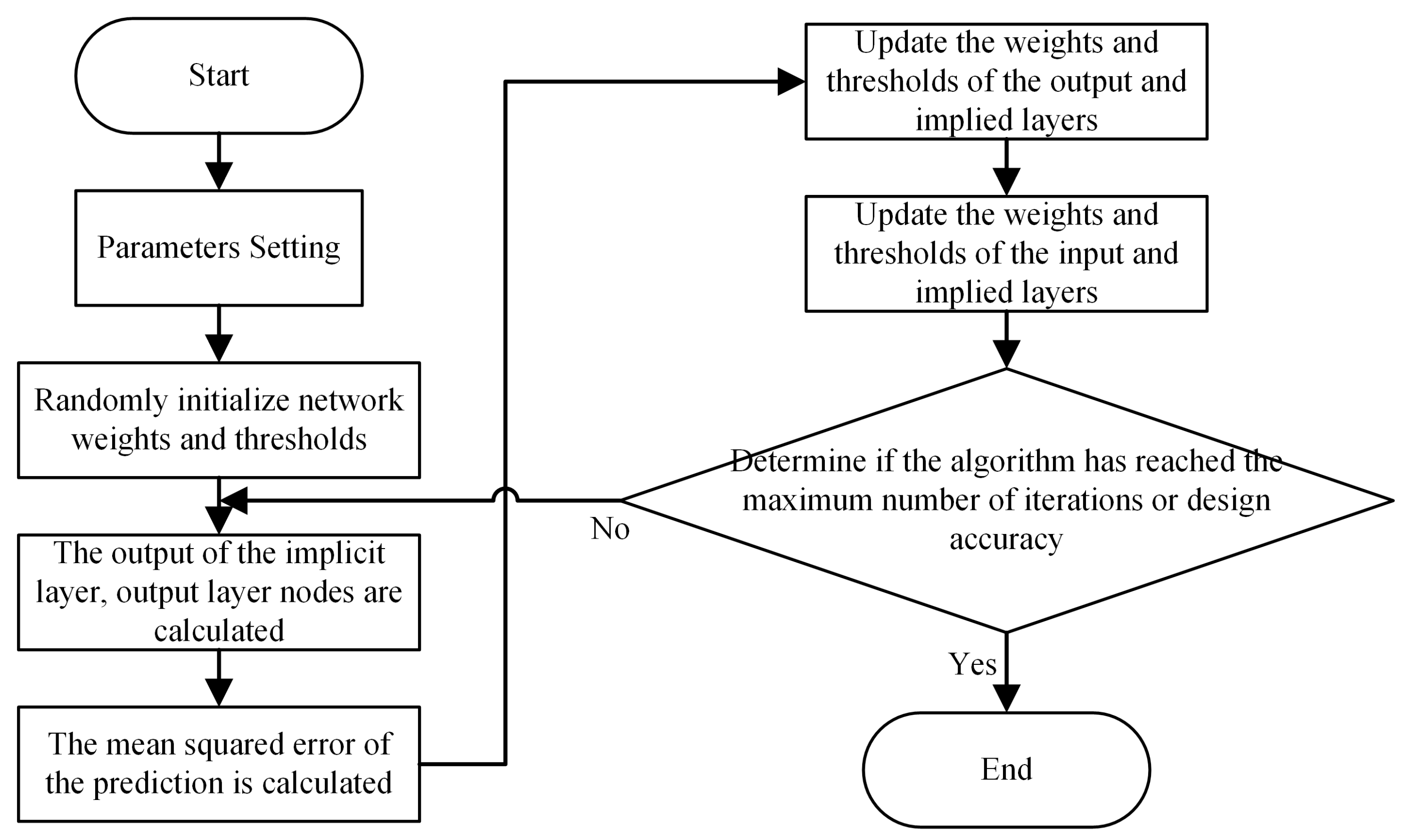
2.1. The Principle of BP Neural Network

The standard BP neural network is divided into two main parts: The first part is forward information transmission, which is the forward transmission of the input information according to the input layer, the hidden layer, and the output layer. The second part is the backward signal propagation, which is the backpropagation method to modify the weights of each layer connection according to the error between the actual value and the predicted value [21,22]. The concrete implementation is shown in Figure 1.

As can be seen from Figure 1, the initial weights and thresholds of the BP neural network are randomly generated. Moreover, the parameters are generally updated by using the gradient descent method. Such a working mechanism makes the BP neural network extremely sensitive to the initial weights, which increases the algorithm’s solving difficulty and convergence time. The initial weights and thresholds of the BP neural network are optimized using the NAGGWO algorithm, which improves its stability and accuracy.

2.2. The Traditional GWO Algorithm

The GWO was first proposed as a swarm intelligence optimization algorithm by Mirjalili et al. [23] in 2014. Gray wolves rely on a clear division of labor and cooperation to hunt and have a clear social dominance hierarchy. The gray wolf population is divided into four levels. The leading gray wolf is called the α wolf, and it is the optimal individual in the group. The next best individual is the β wolf, and the third best is the δ wolf. They represent the direction of the whole wolf group moving forward. The remaining gray wolves of the lower rank are called the ω wolves. The wolves update their positions with Equations (1) and (2) to surround the prey as follows:

$$\overrightarrow{D}=\left|\overrightarrow{C}\times \overrightarrow{X_p^t}-\overrightarrow{X^t}\right|$$

(1)

$$\overrightarrow{X^{t+1}}=\overrightarrow{X_p^t}-\overrightarrow{A}\times \overrightarrow{D}$$

(2)

where t denotes the number of current iterations; $\overrightarrow{X_p^t}$ is the position vector of the prey; $\overrightarrow{X^t}$ is the position vector of the gray wolf; $\overrightarrow{A}$ and $\overrightarrow{D}$ are the coefficient vector, and it is expressed using Equations (3)–(5) as follows:

$$\overrightarrow{A}=2\overrightarrow{a}\times \overrightarrow{r_1}-\overrightarrow{a}$$

(3)

$$\overrightarrow{C}=2\times \overrightarrow{r_2}$$

(4)

$$a=2-2\left(\frac{t}{T_{\mathit{max}}}\right)$$

(5)

where $T_{\mathit{max}}$ denotes the maximum number of iterations; a is the control coefficient that gradually and linearly decreases from 2 to 0; $\overrightarrow{r_1}$ and $\overrightarrow{r_2}$ are random variables whose values are in the range of [0, 1].

It is difficult to determine the prey location in a realistic problem, which is the exact location of optimal solutions. The α wolf, β wolf, and δ wolf are assumed to have excellent prey recognition. The other gray wolves update their position by the position of The α wolf, β wolf, and δ wolf, as shown in Equations (6)–(12).

$$D_{\alpha }=\left|C_1\times X_{\alpha }^t-X^t\right|$$

(6)

$$D_{\beta }=\left|C_2\times X_{\beta }^t-X^t\right|$$

(7)

$$D_{\delta }=\left|C_3\times X_{\delta }^t-X^t\right|$$

(8)

$$X_1=X_{\alpha }-A_1\times D_{\alpha }$$

(9)

$$X_2=X_{\beta }-A_2\times D_{\beta }$$

(10)

$$X_3=X_{\delta }-A_3\times D_{\delta }$$

(11)

$$X^{t+1}=\frac{X_1+X_2+X_3}{3}$$

(12)

2.3. The NAGGWO Algorithm

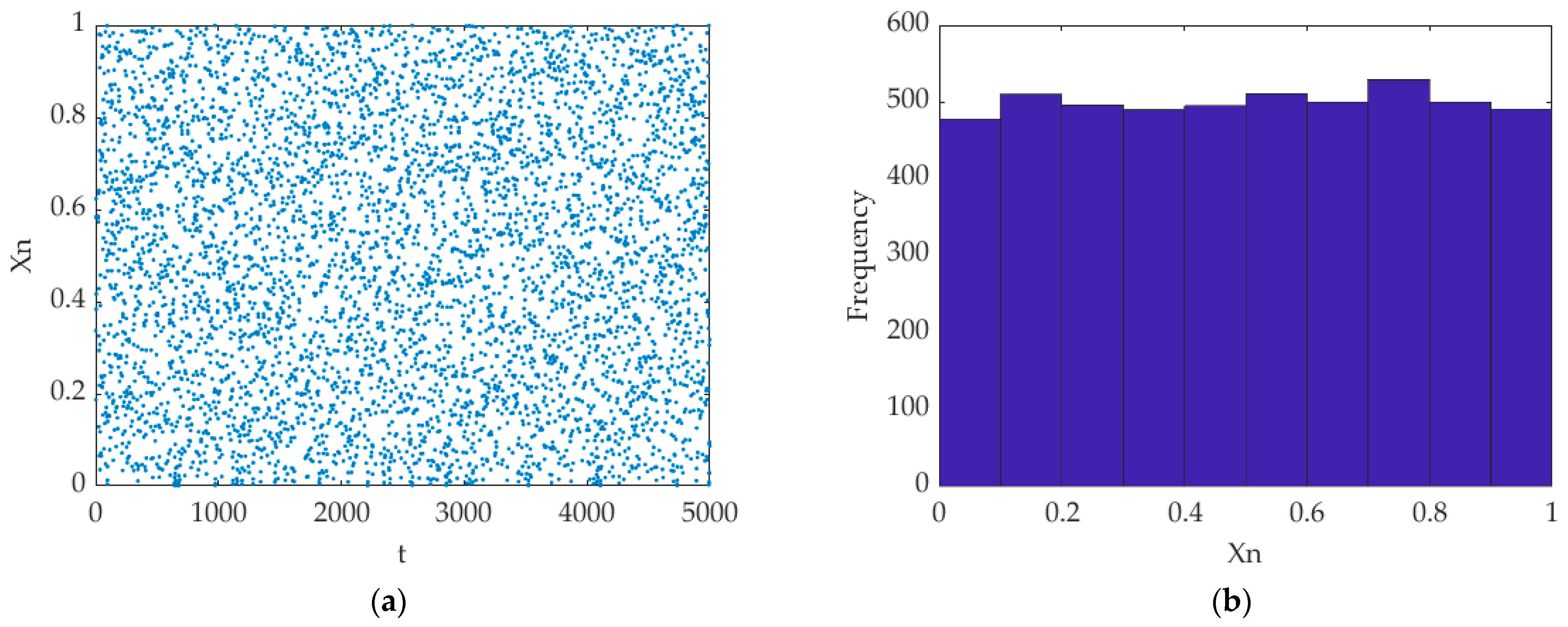
2.3.1. Initialization of CPM Mapping

The GWO algorithm usually uses randomly generated data as the initial population, which easily leads to uneven distribution of the initial population, affects the convergence speed of wolves, and reduces the diversity of the algorithm. To solve this problem, we propose CPM mapping to initialize the population.

Chaotic motions have the characteristics of randomness and ergodicity. When solving optimization problems, the characteristic can ensure population diversity and improve the global search capability of the algorithm. Chaotic mappings include logistic mapping, piecewise mapping, etc. Logistic mapping is widely used in initializing intelligent algorithms [24,25], but its frequency is high in the ranges of [0, 0.1] and [0.9, 1], so the generated initial solutions are often not completely dispersed. Piecewise mapping has a more uniform distribution, but its system loses the chaos at x = 0.5. CPM mapping is proposed to improve it. The mathematical expression is shown in Equation (13) as follows:

$$x_{n+1}=\{\begin{array}{l}\mathit{mod}\left(\left(\frac{x_n}{d}+\mathit{cos}\left(n{\mathit{cos}}^{-1}\left(x_n\times \pi \right)\right)\right),1\right),0\le x_n<d\\ \mathit{mod}\left(\left(\frac{x_n-d}{0.5-d}+\mathit{cos}\left(n{\mathit{cos}}^{-1}\left(x_n\times \pi \right)\right)\right),1\right),d\le x_n<0.5\\ \mathit{mod}\left(\left(\frac{1-d-x_n}{0.5-d}+\mathit{cos}\left(n{\mathit{cos}}^{-1}\left(x_n\times \pi \right)\right)\right),1\right),0.5\le x_n<1-d\\ \mathit{mod}\left(\left(\frac{1-x_n}{d}+\mathit{cos}\left(n{\mathit{cos}}^{-1}\left(x_n\times \pi \right)\right)\right),1\right),1-d\le x_n<1\end{array}$$

(13)

where d is the control parameter taking values in the range (0,1). CPM mapping is performed by combining the piecewise mapping method [26] with the Chebyshev mapping method [27] followed by mod operation. It makes the system chaotic even at x = 0.5. The results of several experiments show that the distribution of the system is relatively uniform for any value of d. It can be used to generate the algorithm’s initial solution and enhance the population’s diversity. The initialized population (one-dimensional) distribution when d = 0.3 is shown in Figure 2.

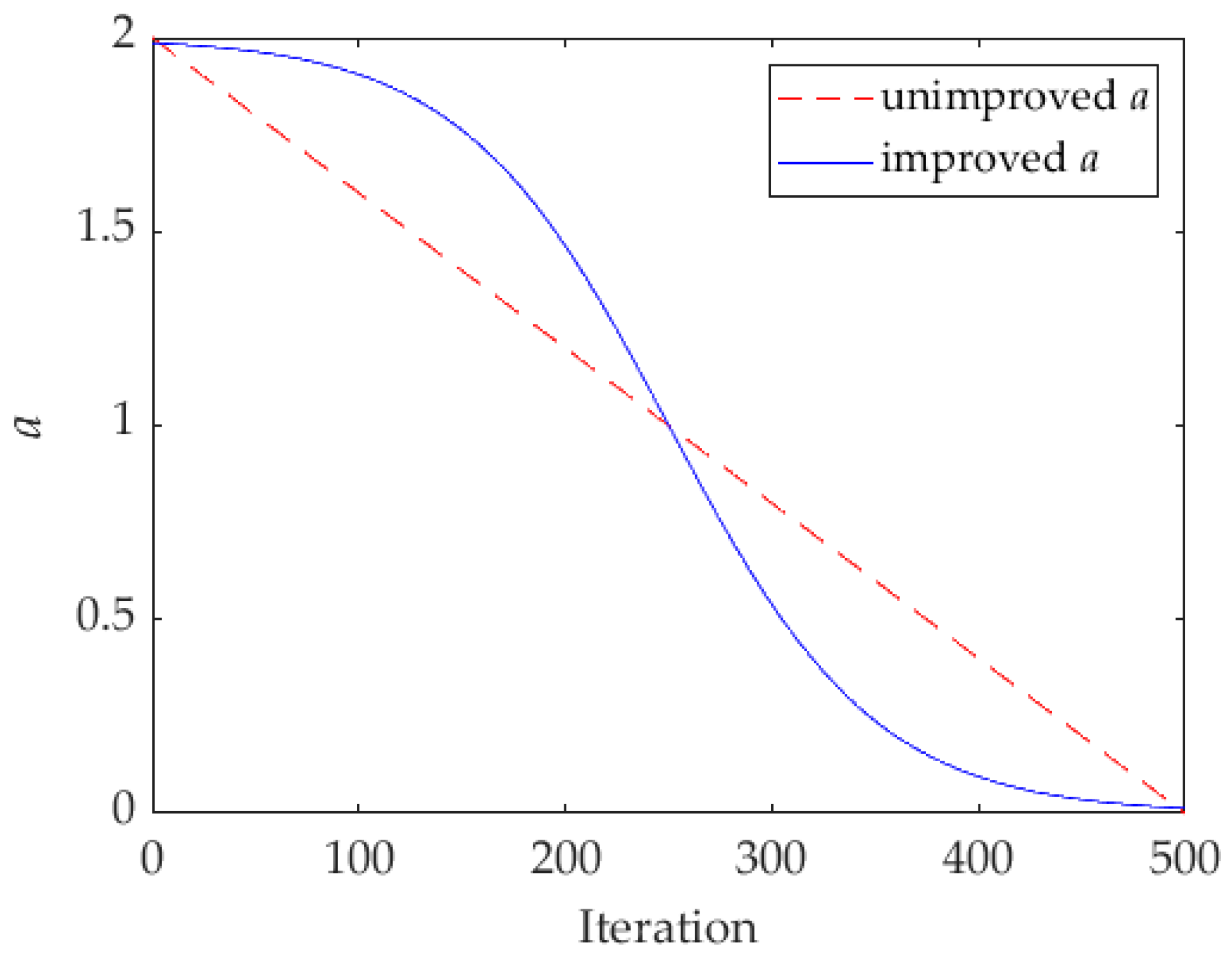
2.3.2. The Nonlinear Control Parameter Adjustment Strategy

The GWO is divided into two steps: prey localization and gray wolf predation. As shown by Equation (2), coefficient A plays a vital role in balancing the global search and local exploitation of the GWO algorithm. When $\left|A\right|>1$, the wolves will expand the search area. When $\left|A\right|<1$, the wolves will narrow the search area and attack the prey. The convergence parameter a influences the magnitude of coefficient A. The value of a linearly decreases with the number of iterations. The convergence parameter a of the linear update is difficult to adapt to the actual search situation due to the complexity of the GWO algorithm’s search process. It cannot achieve strong coordination between global search and local search. Therefore, an ‘S’-type nonlinear control parameter is proposed. The mathematical model is shown in Equation (14).

$$a=2-\frac{2}{1+e^{\left(-\frac{10}{T_{\mathit{max}}}\right)\times \left(t-\frac{T_{\mathit{max}}}{2}\right)}}$$

(14)

The proposed control parameter a slowly decreases in the early iterations, which enables the wolves to search for prey at a large pace and expand the search range of the algorithm. Parameter a rapidly decreases in the middle period, improving the algorithm’s convergence speed. Moreover, parameter a decreases at a slow velocity and maintains a small value in the later stage, which enables the algorithm to fully search around the optimal solution and improves the algorithm’s local search capability. The improved control parameter a can better balance the global and local search and improve the algorithm’s performance. The comparison of the control parameter a before and after the improvement is shown in Figure 3.

2.3.3. The Adaptive Grouping Strategy

Since different individuals of the GWO algorithm are located in different positions, the wolves are divided into three groups according to their distance from the prey (size of fitness value). They are named the predator group, the wanderer group, and the searcher group. Since it is uncertain whether the found prey is the optimal global solution, the individuals closer to the prey should quickly approach it. At the same time, the individuals farther away from the prey are slow to approach the prey or even ignore it to research for other possible prey due to the uncertainty. The individuals with high fitness values are closer to the prey, which accelerates their approach toward the prey for predation. The improved differential evolution strategy is used for position updating to enhance the convergence ability of the algorithm. The individuals with general fitness values are far from the prey, and they wander slowly toward the prey and search the surrounding environment while approaching the prey. Their searching capability is enhanced by combining the GWO position update strategy with stochastic opposition-based learning.. The individuals with poor fitness values, i.e., those farthest from the prey, choose to expand their search range to find other prey. The oscillatory perturbation operator is used for position updating to enhance the ability of the algorithm to jump out of the local optimum. The grouping mathematical model is shown in Equation (15) as follows:

$$X_{i,j}=\{\begin{array}{l}{X}_{i,a},1\le a<n_1\\ X_{i,b},n_1\le a<n_2\\ X_{i,c},n_2\le a\le N\end{array}$$

(15)

where $X_{i,a},X_{i,b},X_{i,c}$ denote the individuals in the predator, wanderer, and searcher groups. n is the number of gray wolves. $n_1$ and $n_2$ are the grouping boundaries. In other words, the wolves are ranked according to their fitness values, with the best individuals in the predator group, the general individuals in the wanderer group, and the poor individuals in the searcher group. $n_1$ and $n_2$ are calculated as shown in Equation (16).

$$\{\begin{array}{l}{n}_1=\frac{1}{4}N\left(1-\frac{t}{T_{\mathit{max}}}\right)\\ n_2=N-\frac{1}{4}N\left(\frac{t}{T_{\mathit{max}}}\right)\end{array}$$

(16)

It can be seen that the grouping boundaries of wolves are adaptively updated with the iteration. At the beginning of the iteration, the convergence speed should be increased because the wolves are dispersed. The predator group can quickly converge to the current optimal solution, so there are more individuals in the predator group in the early stage. As the iteration proceeds, the wolves tend to converge, and it is more necessary to jump out of the local optimum. The searcher group can have a larger search range, so the number of individuals in the searcher group increases as the iteration progresses.

2.3.4. The Position Updating Strategy for Different Groups

The Improved Differential Evolution Strategy

The improved differential evolution strategy is used to update the position of the wolves in the predator group. The differential evolution strategy is an algorithm that evolves based on individual differences in the population [28]. It is widely used in intelligence optimization algorithms [29,30]. In the process of population evolution, individuals are recombined according to their differences from each other to obtain a more competitive intermediate population. The offspring individuals in the intermediate population compete with the parent individuals to produce a more competitive next-generation population. The mutation operation is the most significant part of the differential evolution process. Individual variation is achieved through the differential evolution strategy. A common differential strategy is to randomly select two different individuals, scale their vector differences, and perform vector synthesis with the individual to be mutated. It is calculated using Equation (17) as follows:

$$X_i^{t+1}=X_i^t+W\times \left(X_{r_1}^t-X_{r_2}^t\right)$$

(17)

where $X_i,X_{r_1},X_{r_2}$ denote the three different individuals in the population. W is the scaling factor used to control the scaling scale of the difference vector.

This strategy enables the gray wolves in the predator group to quickly approach the prey by integrating the idea of differential evolution into the GWO algorithm to improve the predator group’s hunting speed. It is the basis of ensuring population competitiveness that the wolves evolve in a good direction according to their environment. Therefore, outstanding gray wolf individuals with high competitiveness are selected as the parents of the evolving population. The expression of its variation function is based on Equation (18) as follows:

$$X_i^{t+1}=X_{\alpha }^t+W\times \left(\frac{X_{\beta }^t}{2}+\frac{X_{\delta }^t}{2}-X_i^t\right)$$

(18)

where W is the scaling factor with the value range of [−1, 1]. It can be seen that the strategy allows the predator group to quickly approach the immediate area of the prey. The algorithm’s convergence ability is greatly enhanced.

The Stochastic Opposition-Based Learning

The position updating strategy of the GWO algorithm is used to update the individuals of the wanderer group. The opposition-based learning was introduced by Tizhoosh [31]. This strategy is widely used in swarm intelligence optimization algorithms and has achieved good experimental results [32,33]. Stochastic opposition-based learning is added to enhance the global search capability of the GWO. The stochastic reverse solution is calculated using Equation (19) as follows:

$$x_{i,j}^{’}=U{B}_j+L{B}_j-r_3\cdot x_{i,j}$$

(19)

where $r_3$ is the random factor taking values in the range of [0, 1]. $U{B}_j$ and $L{B}_j$ are the upper and lower bounds of the j-dimensional values. Compared with general opposition-based learning, the new solutions obtained through stochastic opposition-based learning are dynamic and can increase the diversity of the algorithm. The better individual found through the GWO position updating strategy and the stochastic opposition-based learning is retained in the wanderer group’s position iteration.

The Oscillation Perturbation Operator

The searcher group in the adaptive grouping introduces the oscillatory perturbation operator to increase the algorithm’s diversity and improve the ability of the GWO to jump out of the optimal local solution. The mathematical model of the oscillation operator ξ is shown in Equation (20).

$$\xi =\{\begin{array}{l}\frac{2\sqrt{r_4}-1}{r_5},ift<\frac{T_{\mathit{max}}}{2}\\ 2\sqrt{r_4}-1,ift\ge \frac{T_{\mathit{max}}}{2}\end{array}$$

(20)

where $r_4$ and $r_5$ are the random numbers in the range of [0, 1]. From Equation (20), it can be seen that the oscillation operator takes a large value in the early stage of algorithm iteration, which improves the range of the algorithm’s exploration and increases the algorithm’s diversity. Later in the algorithm iteration, a small oscillation factor is beneficial to increase the algorithm’s development capability. The searcher group’s position updating formula after introducing the oscillation perturbation operator is shown in Equation (21).

$$X_i^{t+1}=\frac{t}{T_{\mathit{max}}}{X}_i^t+\left(1-\frac{t}{T_{\mathit{max}}}\right)\times X_i^t\times \xi$$

(21)

Equation (21) contains the original population information and the part of the oscillatory perturbation, which adaptively varies with the number of iterations. Its position update is not affected by the prey position, which can effectively prevent the algorithm from falling into local extreme points.

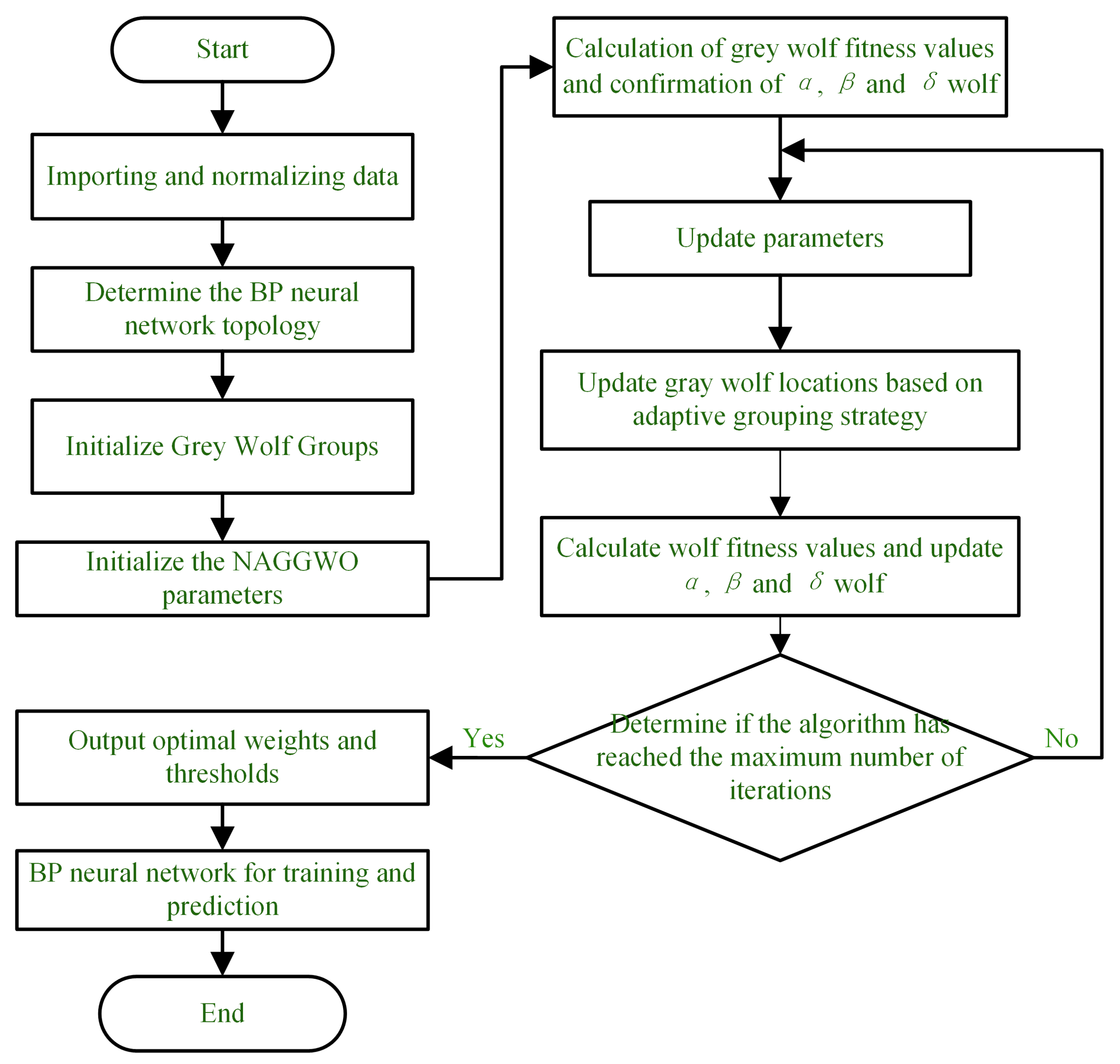
2.4. The NAGGWO-BP Algorithm

The BP neural network model randomly assigns weights and thresholds, which have many variable parameters, leading to unstable model computation [34]. The model prediction performance can be improved by optimizing the BP neural network using the GWO [35]. However, the GWO algorithm has the problems of uneven initial population distribution, slow convergence speed, and easily falling into local optimization. To solve these problems, we propose the NAGGWO algorithm. We first ensure the diversity of the initial gray wolf individuals by introducing CPM mapping. Secondly, we use the ‘S’-type nonlinear control parameter to effectively balance the local and global searching ability and improve the algorithm’s operation efficiency. Finally, we use the adaptive grouping strategy to group the wolves and adopt different updating methods for the individuals in different groups to improve the algorithm’s convergence speed and global searching ability.

The core idea of the NAGGWO-optimized BP neural network is to use the weights and thresholds of the BP neural network as the gray wolf location information. Updating the location is equal to updating the weights and thresholds of the BP neural network until the globally best location is found, which improves the prediction ability and prediction efficiency of the BP neural network. With the introduction of the NAGGWO algorithm, the weights and thresholds of the BP neural network can be dynamically optimized to achieve better and more stable prediction results. The flowchart of the NAGGWO-BP algorithm is shown in Figure 4. First, we normalize the data using Equation (22). Then, we apply CPM mapping, as shown in Equation (13), to initialize the gray wolf population location. Further, the algorithm control parameter a is updated according to Equation (14), and then the individuals are grouped according to the adaptive grouping strategy, and the corresponding positions are updated as in Equations (15)–(21). Finally, the optimal solution is output when the number of iterations reaches the maximum value, and the optimal weights and thresholds of the BP neural network are obtained.

3. Experimental Analysis

3.1. Data Preprocessing

The experimental data were obtained from the literature [17]. In this analysis, we examined the mechanical properties of 88 groups of wood after heat treatment under different conditions. The experimental data on the mechanical properties of these 88 groups are shown in

Table A1. Wood treatment conditions and corresponding mechanical properties.

Test Temperature/°C	Test Time/h	Test Humidity/%	Axial Compressive Strength/MPa	Bending Strength/MPa	Bending Modulus of Elasticity/GPa	Radial Hardness/MPa	Tangential Hardness/MPa
120	0.5	0	39.2	67.4	9.093	14.12	15.56
120	0.5	40	39.1	65.3	9.038	13.02	14.69
120	0.5	60	38.0	69.7	9.100	14.67	15.08
120	0.5	100	36.7	67.2	8.845	14.65	15.45
120	1.0	0	38.4	67.8	8.649	13.98	14.36
120	1.0	40	37.6	66.4	8.752	12.98	15.59
120	1.0	60	38.6	67.8	9.245	13.78	15.32
120	1.0	100	38.1	63.1	7.895	14.55	14.23
120	2.0	0	39.5	66.9	9.074	13.33	14.23
120	2.0	40	38.6	68.2	8.945	12.55	14.58
120	2.0	60	36.5	65.2	8.854	13.25	14.89
120	2.0	100	41.9	63.2	8.933	13.36	14.56
120	3.0	0	37.5	66.5	8.900	13.56	14.78
120	3.0	40	39.8	67.6	8.963	13.45	14.45
120	3.0	60	37.6	66.6	8.745	13.01	14.69
120	3.0	100	38.9	64.2	8.745	12.45	14.78
140	0.5	0	36.7	66.7	8.978	14.69	15.56
140	0.5	40	36.9	67.5	8.845	13.06	15.02
140	0.5	60	35.8	66.8	9.155	14.02	14.23
140	0.5	100	38.4	65.3	8.877	15.02	15.01
140	1.0	0	37.4	66.5	9.179	14.16	15.68
140	1.0	40	36.0	64.5	9.137	13.05	15.01
140	1.0	60	37.2	67.2	9.024	13.49	15.17
140	1.0	100	37.5	63.1	8.823	13.45	15.48
140	2.0	0	37.9	66.3	8.823	13.54	14.69
140	2.0	40	38.5	65.7	8.852	14.69	14.58
140	2.0	60	37.6	67.1	8.799	13.99	14.74
140	2.0	100	35.5	62.7	8.900	14.28	15.63
140	3.0	0	36.9	65.4	8.811	14.39	14.23
140	3.0	40	38.9	64.6	8.934	13.23	14.56
140	3.0	60	38.2	65.5	8.654	14.23	13.65
140	3.0	100	39.2	62.1	8.798	13.56	14.02
160	0.5	0	36.9	66.3	8.788	14.89	14.99
160	0.5	40	39.1	66.9	9.011	14.87	14.36
160	0.5	60	37.1	66.3	8.745	14.58	14.78
160	0.5	100	38.9	65.8	8.712	14.69	15.69
160	1.0	0	39.1	62.4	8.679	13.42	14.56
160	1.0	40	39.7	61.4	8.645	14.09	15.30
160	1.0	60	37.8	62.2	8.798	14.69	15.90
160	1.0	100	38.7	62.8	8.679	13.58	15.63
160	2.0	0	35.9	62.2	8.727	14.63	13.92
160	2.0	40	35.8	62.1	8.557	14.02	14.17
160	2.0	60	36.6	63.1	8.687	15.17	14.28
160	2.0	100	38.2	60.9	8.611	14.65	15.09
160	3.0	0	37.2	61.9	8.611	13.65	14.36
160	3.0	40	39.1	61.5	8.534	13.47	14.56
160	3.0	60	39.5	60.8	8.601	13.58	13.89
160	3.0	100	37.3	60.5	8.552	13.69	14.36
180	0.5	0	38.9	65.9	8.601	15.21	14.03
180	0.5	40	39.1	65.3	8.689	15.98	14.56
180	0.5	60	37.6	66.1	8.645	16.01	13.97
180	0.5	100	36.1	65.7	8.599	14.32	14.33
180	1.0	0	38.2	65.4	8.623	15.09	13.79
180	1.0	40	39.4	64.9	8.645	14.98	14.25
180	1.0	60	37.6	66.3	8.579	15.45	14.08
180	1.0	100	38.1	64.8	8.545	14.33	13.64
180	2.0	0	39.5	65.1	8.574	14.65	13.69
180	2.0	40	38.7	65.8	8.600	14.13	13.59
180	2.0	09	38.2	64.5	8.532	13.99	14.49
180	2.0	100	37.1	64.2	8.544	15.10	13.54
180	3.0	0	38.1	64.1	8.600	14.21	14.06
180	3.0	40	37.5	64.2	8.541	13.99	14.21
180	3.0	60	37.8	64.8	8.456	14.58	13.98
180	3.0	100	38.5	63.8	8.499	14.99	13.69
200	0.5	0	36.5	62.1	8.483	12.00	13.60
200	0.5	40	35.4	60.6	8.475	11.96	12.99
200	0.5	60	35.1	59.9	8.399	11.45	13.21
200	1.0	0	34.5	61.9	8.422	11.69	12.98
200	1.0	40	35.8	60.8	8.489	11.46	12.64
200	1.0	60	34.1	61.2	8.321	11.54	12.35
200	2.0	0	34.6	61.2	8.369	11.99	13.02
200	2.0	40	35.4	60.8	8.354	11.15	12.69
200	2.0	60	34.5	60.5	8.211	10.65	12.49
200	3.0	0	34.1	60.9	8.249	10.68	12.73
200	3.0	40	34.2	59.8	8.231	11.05	12.57
200	3.0	60	33.8	58.2	8.011	10.22	12.37
210	0.5	0	34.1	50.1	7.856	10.23	10.98
210	0.5	40	33.2	50.8	7.789	10.59	9.98
210	0.5	60	32.1	49.9	7.865	10.55	10.23
210	1.0	0	33.9	50.6	7.765	10.21	10.65
210	1.0	40	32.9	49.8	7.712	9.98	10.21
210	1.0	60	32.8	48.9	7.498	10.01	10.65
210	2.0	0	32.9	49.1	7.689	9.98	9.64
210	2.0	40	32.5	49.5	7.712	9.65	9.35
210	2.0	60	31.8	49.6	7.623	10.03	9.67
210	3.0	0	31.5	47.8	7.500	9.21	8.91
210	3.0	40	30.5	46.5	7.412	9.10	8.21
210	3.0	60	30.8	45.1	7.321	9.03	8.99

in Appendix A.

The material used for this experiment was 22 mm larch from northeastern China. The wood was heat-treated via steam at a temperature of 120–210 °C and relative humidity of 0–100% for 0.5–3 h. The treated wood was dried to reach the moisture content of 8–10% and placed at the ambient temperature of 20 °C with a relative humidity level of 65%. After equilibrium, the corresponding mechanical properties were measured. The experimental results are consistent with the conclusions reached by Ding et al. [36] and Tiryaki et al. [37]. This proves that the experimental data are accurate and reliable.

We used the same training and testing specimens as those found in the literature [38] to ensure the fairness of the model comparison. The first 58 sets of experimental data in Appendix A Table A1 were used as the training set, and the last 30 sets of experimental data were classified as the testing set. Since the magnitudes of the three input dimensions are different, Equation (22) is used to normalize the input data to avoid the effect of direct input on the training speed and prediction accuracy of the prediction model.

$$y=\left(y_{\mathit{max}}-y_{\mathit{min}}\right)\times \frac{\left(x-x_{\mathit{min}}\right)}{\left(x_{\mathit{max}}-x_{\mathit{min}}\right)}+y_{\mathit{min}}$$

(22)

where y is the normalized value of x, and $y_{\mathit{min}}$, $y_{\mathit{max}}$ are the normalized intervals set to −1, 1. $x_{\mathit{min}}$ and $x_{\mathit{max}}$ are the minimum and maximum values of x, respectively.

3.2. Model Parameter Setting

The BP neural network in the NAGGWO-BP model uses the three-layer structure. The number of nodes in its input layer is 3, corresponding to the input data’s temperature, humidity, and time. The number of nodes in the output layer is 1, which corresponds to the mechanical properties of wood. The number of hidden layer nodes is generally selected based on the empirical Equation (23). The range of the hidden layer nodes is calculated to be [3,12]. After several error calculations, the number of nodes in the hidden layer is confirmed to be 9.

$$h=\sqrt{\left(u+v\right)}+w,w\in \left[1,10\right]$$

(23)

where h, u, and v denote the number of nodes at the hidden, input, and output layers, respectively.

The NAGGWO-BP model was used to predict the mechanical properties of wood. The predicted results were compared with those of the BP, GWO-BP, and TSSA-BP neural networks to verify the model’s prediction performance. The BP neural network’s maximum number of iterations was 1000; the target error was 0.0001; the maximum number of iterations was 50, and the population size was 20.

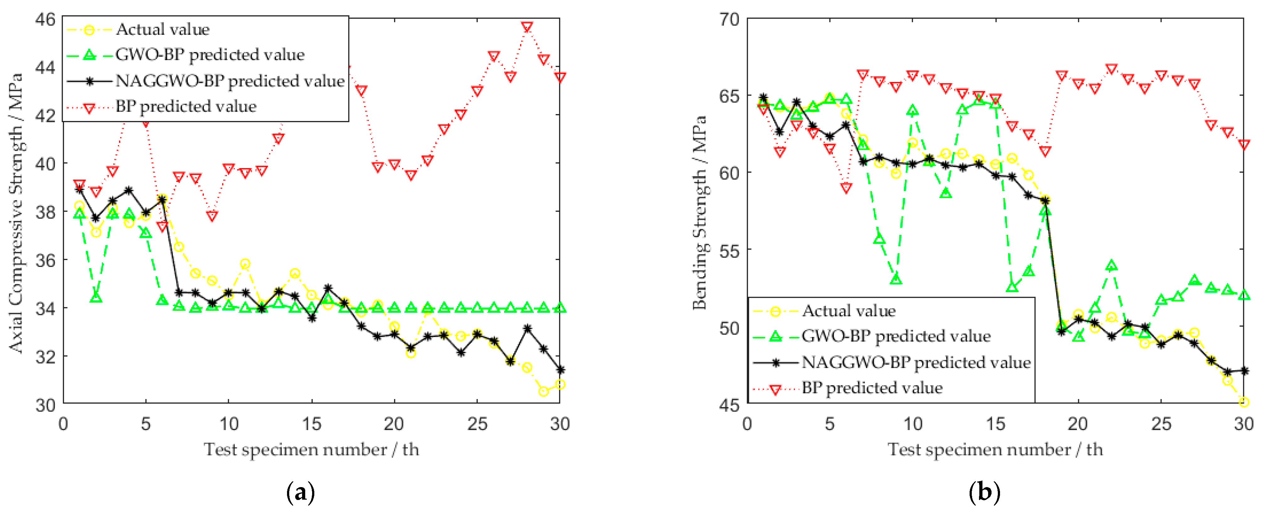
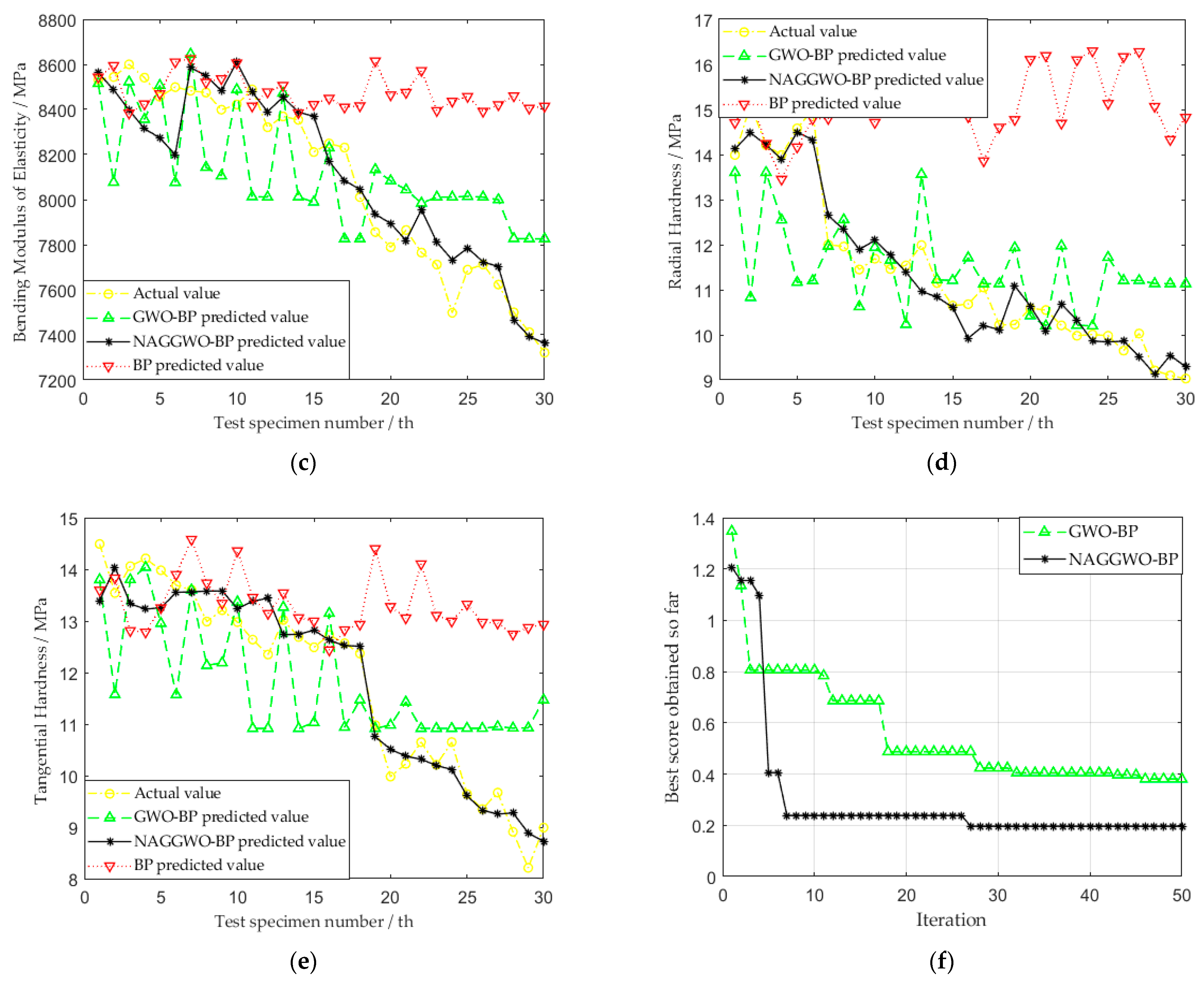
3.3. NAGGWO-BP Simulation Results Analysis

To verify the effectiveness of the NAGGWO-BP, the mean absolute error (MAE), the mean square error (MSE), and the mean absolute percentage error (MAPE) of the different algorithms were compared to evaluate their prediction performance. Smaller values indicate better model prediction performance. The experimental results are shown in

Table 2. Model and error quantity.

	NAGGWO-BP			GWO-BP			BP			TSSA-BP
	MAE	MSE	MAPE	MAE	MSE	MAPE	MAE	MSE	MAPE	MAE	MSE	MAPE
Axial Compressive Strength	0.65	0.73	1.90%	1.26	2.80	3.72%	6.99	63.14	20.98%	1	1.48	2.90%
Bending Strength	0.79	0.99	1.38%	2.57	12.48	4.72%	8.58	113.37	16.67%	3.68	16.99	6.81%
Bending Modulus of Elasticity	103.52	16,174	1.27%	272.20	94,416	3.41%	406.44	289,351	5.25%	282.56	235,795	3.12%
Radial Hardness	0.37	0.21	3.27%	1.21	2.66	10.51%	3.90	19.32	37.39%	0.66	0.66	5.64%
Tangential Hardness	0.39	0.25	3.29%	1.10	1.74	9.98%	1.78	5.23	17.36%	0.99	1.57	9.61%

, and the TSSA-BP data were obtained from the literature [38].

BP denotes the original backpropagation neural network. NAGGWO-BP, GWO-BP, and TSSA-BP denote the BP neural network after its optimization using the NAGGWO, GWO [23], and TSSA [38] models. As shown in Table 1, the MAE, MSE, and MAPE values of the NAGGWO-BP neural network prediction model are much smaller than the prediction errors of other models. The MAE of NAGGWO-BP is reduced by 74.5–90.7%, MSE by 94.4–99.1%, and MAPE by 4.0–34.1%, compared with those of the BP neural network. This indicates that combination with NAGGWO can optimize the BP neural network performance to a great extent. The other algorithms are also optimized for the BP neural network but are still significantly inferior to the proposed NAGGWO algorithm. This indicates that compared with the BP, GWO-BP, and TSSA-BP models, the NAGGWO-BP neural network is more reasonable and has better prediction ability.

Figure 5a–e show the prediction results of the NAGGWO-BP, GWO-BP, and BP neural networks for five mechanical properties of wood. The predicted values of the optimized BP neural network using GWO and NAGGWO are closer to the actual values, indicating that using GWO and NAGGWO can significantly improve the prediction accuracy of the BP neural network. However, it can be seen that using NAGGWO is more effective. In addition, Figure 5f shows the convergence curves of the GWO and NAGGWO models in terms of compressive strength along the grain. It can be seen that the NAGGWO model is superior to the GWO model in terms of convergence speed and convergence accuracy and often achieves better results after 10 iterations. The analysis of the reasons for this is as follows: (1) The CPM mapping process used by the NAGGWO algorithm initializes the wolf population, which improves the diversity of the algorithm and establishes a good foundation for the optimization search afterward. (2) The NAGGWO algorithm proposes the adaptive grouping strategy, divides the population into three parts according to the fitness size, and uses different position updating strategies for individuals in different positions, improving the algorithm’s search accuracy. This can optimize the BP neural network’s parameters to the maximum extent and improves its prediction ability. (3) The improved differential evolution strategy is used for the predator group so that it can quickly approach the optimal solution, which effectively improves the convergence speed of the algorithm. Meanwhile, the proposed nonlinear control parameter a keeps large values in the early stage, which gives the algorithm good global searching ability in the early stage. Hence, the algorithm tends to converge to the optimal solution more quickly. It can be proved that the proposed NAGGWO-BP is a prediction model with excellent performance.

4. Conclusions

The thermal modification of wood is a very complex and nonlinear process. The wood structure is complex, and its chemical composition is prone to change. Therefore, establishing an ideal mathematical model in line with the actual situation is the prerequisite for the automated control of the thermal modification of wood and an effective way to reduce and improve wood consumption. For the mechanical properties of wood thermal modification, the NAGGWO-BP prediction model was established, and the prediction of Chinese larch’s mechanical properties was studied. The main conclusions are as follows:

• The NAGGWO algorithm is proposed to solve the problem that the traditional GWO algorithm tends to fall into the local optimum. Firstly, the population is initialized by using CPM mapping. Secondly, an ‘S’-type nonlinear control parameter is proposed to balance the exploration and exploitation ability of the algorithm. Finally, different search methods are used for different groups of wolves by adaptively grouping them according to their fitness size. The solving speed and accuracy of the algorithm are improved.
• The proposed NAGGWO-BP model updates the weights and thresholds of the BP neural network using the NAGGWO algorithm to address the problem of its imprecise prediction results. It enhances the prediction ability of the BP neural network. We applied the NAGGWO-BP model to predict the five mechanical properties of wood to validate the model. The results show that the MAE, MSE, and MAPE values of the NAGGWO-BP model are greatly reduced, compared with the original BP neural network, and the prediction ability of the algorithm is substantially enhanced.

References

1. Esteves, B.; Ferreira, H.; Viana, H.; Ferreira, J.; Domingos, I.; Cruz-Lopes, L.; Jones, D.; Nunes, L. Termite Resistance, Chemical and Mechanical Characterization of Paulownia tomentosa Wood before and after Heat Treatment. Forests 2021, 12, 1114. [Google Scholar] [CrossRef]
2. Suri, I.F.; Purusatama, B.D.; Kim, J.H.; Yang, G.U.; Prasetia, D.; Kwon, G.J.; Hidayat, W.; Lee, S.H.; Febrianto, F.; Kim, N.H. Comparison of physical and mechanical properties of Paulownia tomentosa and Pinus koraiensis wood heat-treated in oil and air. Eur. J. Wood Wood Prod. 2022, 80, 1389–1399. [Google Scholar] [CrossRef]
3. Wang, W.; Ma, W.; Wu, M.; Sun, L. Effect of Water Molecules at Different Temperatures on Properties of Cellulose Based on Molecular Dynamics Simulation. Bioresources 2022, 17, 269–280. [Google Scholar] [CrossRef]
4. Esteves, B.; Marques, A.V.; Domingos, I.; Pereira, H. Heat-induced colour changes of pine (Pinus pinaster) and eucalypt (Eucalyptus globulus) wood. Wood Sci. Technol. 2008, 42, 369–384. [Google Scholar] [CrossRef] [Green Version]
5. Huang, X.; Kocaefe, D.; Kocaefe, Y.; Boluk, Y.; Pichette, A. A spectrocolorimetric and chemical study on color modification of heat-treated wood during artificial weathering. Appl. Surf. Sci. 2012, 258, 5360–5369. [Google Scholar] [CrossRef]
6. Navickas, P.; Albrektas, D. Effect of Heat Treatment on Sorption Properties and Dimensional Stability of Wood. Mater. Sci.-Medzg. 2013, 19, 291–294. [Google Scholar] [CrossRef] [Green Version]
7. Bekhta, P.; Niemz, P. Effect of high temperature on the change in color, dimensional stability and mechanical properties of spruce wood. Holzforschung 2003, 57, 539–546. [Google Scholar] [CrossRef]
8. Wang, J.Y.; Cooper, P.A. Effect of oil type, temperature and time on moisture properties of hot oil-treated wood. Holz Als Roh-Und Werkst. 2005, 63, 417–422. [Google Scholar] [CrossRef]
9. Bayani, S.; Taghiyari, H.R.; Papadopoulos, A.N. Physical and Mechanical Properties of Thermally-Modified Beech Wood Impregnated with Silver Nano-Suspension and Their Relationship with the Crystallinity of Cellulose. Polymers 2019, 11, 1538. [Google Scholar] [CrossRef] [Green Version]
10. Herrera-Diaz, R.; Sepulveda-Villarroel, V.; Torres-Mella, J.; Salvo-Sepulveda, L.; Llano-Ponte, R.; Salinas-Lira, C.; Peredo, M.A.; Ananias, R.A. Influence of the wood quality and treatment temperature on the physical and mechanical properties of thermally modified radiata pine. Eur. J. Wood Wood Prod. 2019, 77, 661–671. [Google Scholar] [CrossRef]
11. Cai, X.; Riedl, B.; Zhang, S.Y.; Wan, H. Effects of nanofillers on water resistance and dimensional stability of solid wood modified by melamine-urea-formaldehyde resin. Wood Fiber Sci. 2007, 39, 307–318. [Google Scholar] [CrossRef]
12. Hussain, S.F.; Hussain, G.; Rahman, N. Artificial neural network modelling and optimization of elastic and an-elastic spring back in polymer parts produced through ISF. Int. J. Adv. Manuf. Technol. 2022, 118, 2163–2176. [Google Scholar] [CrossRef]
13. Prikeznik, M.; Srcic, S. Artificial neural networks for investigation of the most important factors of industrial tablet manufacturing on the dissolution of active pharmaceutical ingredients as critical quality attributes. Farmacia 2021, 69, 732–740. [Google Scholar] [CrossRef]
14. Shaik, N.B.; Mantrala, K.M.; Narayana, K.L. Prediction of corrosion properties of LENS (TM) deposited cobalt, chromium and molybdenum alloy using artificial neural networks. Int. J. Mater. Prod. Technol. 2021, 62, 4–15. [Google Scholar] [CrossRef]
15. Wang, C.-S.; Hsiao, Y.-H.; Chang, H.-Y.; Chang, Y.-J. Process Parameter Prediction and Modeling of Laser Percussion Drilling by Artificial Neural Networks. Micromachines 2022, 13, 529. [Google Scholar] [CrossRef]
16. Zhang, D.; Liu, Y.; Cao, J.; Sun, L. Neural Network Prediction Model of Wood Moisture Content for Drying Process. Sci. Silvae Sin. 2008, 44, 94–98. [Google Scholar] [CrossRef]
17. Yang, H.; Cheng, W.; Han, G. Wood Modification at High Temperature and Pressurized Steam: A Relational Model of Mechanical Properties Based on a Neural Network. Bioresources 2015, 10, 5758–5776. [Google Scholar] [CrossRef]
18. Chai, H.; Chen, X.; Cai, Y.; Zhao, J. Artificial Neural Network Modeling for Predicting Wood Moisture Content in High Frequency Vacuum Drying Process. Forests 2019, 10, 16. [Google Scholar] [CrossRef] [Green Version]
19. Hadavandi, E.; Mostafayi, S.; Soltani, P. A Grey Wolf Optimizer-based neural network coupled with response surface method for modeling the strength of siro-spun yarn in spinning mills. Appl. Soft Comput. 2018, 72, 1–13. [Google Scholar] [CrossRef]
20. Tian, Y.; Yu, J.; Zhao, A. Predictive model of energy consumption for office building by using improved GWO-BP. Energy Rep. 2020, 6, 620–627. [Google Scholar] [CrossRef]
21. Hu, R.; Wen, S.; Zeng, Z.; Huang, T. A short-term power load forecasting model based on the generalized regression neural network with decreasing step fruit fly optimization algorithm. Neurocomputing 2017, 221, 24–31. [Google Scholar] [CrossRef]
22. Wang, J.; Shi, P.; Jiang, P.; Hu, J.; Qu, S.; Chen, X.; Chen, Y.; Dai, Y.; Xiao, Z. Application of BP Neural Network Algorithm in Traditional Hydrological Model for Flood Forecasting. Water 2017, 9, 48. [Google Scholar] [CrossRef] [Green Version]
23. Mirjalili, S.; Mirjalili, S.M.; Lewis, A. Grey Wolf Optimizer. Adv. Eng. Softw. 2014, 69, 46–61. [Google Scholar] [CrossRef] [Green Version]
24. Yan, Y.; Ma, H.; Li, Z. An Improved Grasshopper Optimization Algorithm for Global Optimization. Chin. J. Electron. 2021, 30, 451–459. [Google Scholar] [CrossRef]
25. Lu, Q.Z.; Jiang, J.H.; Yu, R.Q.; Shen, G.L. A genetic algorithm based on prepotency evolution using chaotic initiation used for network training. J. Chem. Inf. Comput. Sci. 2003, 43, 1132–1137. [Google Scholar] [CrossRef]
26. Leriche, R.; Sienra, G. Dynamical Aspects of Piecewise Conformal Maps. Qual. Theory Dyn. Syst. 2019, 18, 1237–1261. [Google Scholar] [CrossRef] [Green Version]
27. Choi, J.-Y.; Im, D.K.; Park, J.; Choi, S. Prediction of Dynamic Stability Using Mapped Chebyshev Pseudospectral Method. Int. J. Aerosp. Eng. 2018, 2018, 2508153. [Google Scholar] [CrossRef]
28. Storn, R.; Price, K. Differential Evolution—A Simple and Efficient Heuristic for global Optimization over Continuous Spaces. J. Glob. Optim. 1997, 11, 341–359. [Google Scholar] [CrossRef]
29. Sun, G.; Yang, B.; Yang, Z.; Xu, G. An adaptive differential evolution with combined strategy for global numerical optimization. Soft Comput. 2020, 24, 6277–6296. [Google Scholar] [CrossRef]
30. Das, S.; Mullick, S.S.; Suganthan, P.N. Recent advances in differential evolution—An updated survey. Swarm Evol. Comput. 2016, 27, 1–30. [Google Scholar] [CrossRef]
31. Tizhoosh, H.R. Opposition-based learning: A new scheme for machine intelligence. In Proceedings of the International Conference on Computational Intelligence for Modelling, Control and Automation and International Conference on Intelligent Agents, Web Technologies and Internet Commerce, Vienna, Austria, 28–30 November 2005. [Google Scholar]
32. Tubishat, M.; Idris, N.; Shuib, L.; Abushariah, M.A.M.; Mirjalili, S. Improved Salp Swarm Algorithm based on opposition based learning and novel local search algorithm for feature selection. Expert Syst. Appl. 2020, 145, 113122. [Google Scholar] [CrossRef]
33. Dhargupta, S.; Ghosh, M.; Mirjalili, S.; Sarkar, R. Selective Opposition based Grey Wolf Optimization. Expert Syst. Appl. 2020, 151, 113389. [Google Scholar] [CrossRef]
34. Bai, H.R.; Chu, Z.Y.; Wang, D.W.; Bao, Y.; Qin, L.Y.; Zheng, Y.H.; Li, F.M. Predictive control of microwave hot-air coupled drying model based on GWO-BP neural network. Dry. Technol. 2022. [Google Scholar] [CrossRef]
35. Liang, Q.; Zhang, X.M.; Liu, X.; Li, Y.L. Prediction of high-temperature flow stress of HMn64-8-5-1.5 manganese brass alloy based on modified Zerilli-Armstrong, Arrhenius and GWO-BPNN model. Mater. Res. Express 2022, 9, 9. [Google Scholar] [CrossRef]
36. Ding, T.; Gu, L.; Li, T. Influence of steam pressure on physical and mechanical properties of heat-treated Mongolian pine lumber. Eur. J. Wood Wood Prod. 2011, 69, 121–126. [Google Scholar] [CrossRef]
37. Tiryaki, S.; Aydin, A. An artificial neural network model for predicting compression strength of heat treated woods and comparison with a multiple linear regression model. Constr. Build. Mater. 2014, 62, 102–108. [Google Scholar] [CrossRef]
38. Li, N.; Wang, W. Prediction of Mechanical Properties of Thermally Modified Wood Based on TSSA-BP Model. Forests 2022, 13, 160. [Google Scholar] [CrossRef]
Figure 1. Flowchart of BP neural network.
Forests 13 01870 g001
Figure 2. Population initialization in CPM mapping: (a) scatter map; (b) frequency distribution histogram.
Forests 13 01870 g002
Figure 3. The changing curve of the convergence parameter a.
Forests 13 01870 g003
Figure 4. Flowchart of NAGGWO-BP algorithm.
Forests 13 01870 g004
Figure 5. Comparison between predicted results and actual values for different models: (a) compressive strength along grain; (b) flexural strength; (c) flexural modulus of elasticity; (d) radial hardness; (e) tangential hardness; (f) convergence curve of GWO-BP and NAGGWO-BP.
Forests 13 01870 g005aForests 13 01870 g005b