Individual-Tree and Stand-Level Models for Estimating Ladder Fuel Biomass Fractions in Unpruned Pinus radiata Plantations

Abstract

The mild climate and, in recent decades, the increased demand for timber have favoured the establishment of extensive plantations of fast-growing species such as Pinus radiata in Galicia (a fire-prone region in northwestern Spain). This species is characterised by very poor self-pruning; unmanaged pine stands have a worrying vertical continuity of fuels after crown closure because the dead lower branches accumulate large amounts of fine dead biomass including twigs and suspended needles. Despite the important contribution of these dead ladder fuels to the overall canopy biomass and to crown-fire hazards, equations for estimating these fuels have not yet been developed. In this study, two systems of equations for estimating dead ladder fuel according to size class and the vertical distribution in the first 6 m of the crown were fitted: a tree-level system based on individual tree and stand variables and a stand-level system based only on stand variables. The goodness-of-fit statistics for both model systems indicated that the estimates were robust and accurate. At the tree level, fuel biomass models explained between 35% and 59% of the observed variability, whereas cumulative fuel biomass models explained between 62% and 81% of the observed variability. On the other hand, at the stand level, fuel-load models explained between 88% and 98% of the observed variability, whereas cumulative fuel-load models explained more than 98% of the total observed variability. These systems will therefore allow managers to adequately quantify the dead ladder fuels in pure Pinus radiata stands and to identify the treatments required to reduce crown-fire hazard.

1. Introduction

Fuel bed, the general term for the complex array of biomass types in a given area, is vertically stratified into three fuel layers: ground, surface, and canopy fuels [1]. Ground fuel comprises all of the burnable material below the litter including duff, plant roots, decaying wood, and peat. Ground fuel supports smouldering (flameless) combustion, which produces lower temperatures and lasts longer than the flaming combustion of surface fuels [2]. Canopy or aerial fuels comprise the biomass above the surface fuel layer; some of their structural characteristics such as canopy fuel load (CFL), canopy bulk density (CBD), and canopy base height (CBH) affect the initiation and spread of crown fires [3,4]. These variables must be quantified to predict fire behaviour characteristics and enable the selection of appropriate silvicultural treatments aimed at reducing susceptibility to crown fires in fire-prone stands such as pine forests [5]. CFL is defined as the mass of available canopy fuel per unit ground area, CBD indicates the amount of available fuel per volume unit in the aerial layer, and CBH is the lowest height above ground level at which there is sufficient canopy fuel to propagate fire vertically through the canopy [6,7]. For modelling purposes, needles and fine twigs (diameter < 6 mm) are usually considered the available fuel because they are generally consumed within the flaming front of a crown fire [8].

Different approaches and methods have been used to estimate the canopy fuel variables related to crown fires; e.g., [3,6,9]. The most commonly used approach is the “load-over-depth method”, which assumes that all canopy fine fuel is homogeneously distributed. This method is consistent with the semi-empirical based models used in the main fire behaviour simulators available [10]. The canopy fine fuel can be estimated at the individual tree level by using equations to predict crown fuel characteristics using regressor variables that are easy to measure in the field such as tree diameter or height; e.g., [11,12]; and at the stand level by using models that are less accurate but also less demanding in terms of sampling. Thus, for example, in the study area, i.e., the north-western Iberian Peninsula, these types of models have been developed for pine stands that are prone to crown fires using stand variables determined in field inventories [11,12,13,14,15,16] or by remote sensing technologies including airborne light detection and ranging (LiDAR) [17,18,19,20] and optical satellite imagery [21]. The latter two approaches are less accurate than those based on field inventory but facilitate landscape-level mapping and thus the use of map-based simulation systems such as FlamMap [22].

The surface fuel layer (including litter, shrubs, grasses, and woody biomass) also contributes to crown-fire hazards because its load (biomass per unit area) modulates the fireline intensity of the surface phase and its height affects the fuel strata gap (FSG), which is defined as the distance from the top of the surface fuel bed to the lower limit of the aerial fuel stratum comprising the ladder and live crown fuels that can support vertical fire propagation [23].

Surface fuels are characterised by similar methods to those described for canopy fuels. However, given the high coverage and complexity of shrub communities with or without an overlaying tree canopy in the study region, the stand-level approach is based on field inventory [24,25], terrestrial laser scanning [26] and remote sensing techniques such as LiDAR [27] and satellite imaging [21].

In Galicia (NW Spain), an area at the intersection between the Mediterranean and Atlantic climatic influences, a certain level of summer drought coexists with high forest productivity, resulting in very high fuel accumulation [28,29]. These favourable site conditions have allowed the proliferation of pure and even-aged pine stands, especially of Pinus pinaster L. and Pinus radiata D. Don. According to the IV National Forest Inventory (IVIFN [30]), these species cover 217,000 and 96,000 ha, respectively, accounting for 15 and 7% of the forest area in the region. The mild climate and, in recent decades, the increased demand for timber have favoured the establishment of extensive commercial forest plantations of both fast-growing species [30,31].

Different silvicultural or forest management strategies are used for these species in Galicia depending on site quality and the cost effectiveness of the final products [32]. These strategies include fuel treatments by thinning and pruning (to a maximum height of 6 m) to reduce canopy fuels and mastication to control surface fuels. These treatments enable a certain vertical and horizontal fuel discontinuity to be maintained by generating a gap between surface and canopy fuels; they are thus expected to decrease the likelihood of crown fire initiation and spread. However, a high proportion of adult pine stands are either not managed or are inadequately managed and display a worrying vertical continuity of fuels. This particularly applies to Pinus radiata stands, given the very poor self-pruning that characterises the species [33]. Thus, large amounts of dead biomass accumulate in the lower canopy after crown closure, including fine twigs and suspended needles, which represent the so-called ladder fuels.

Ladder fuels comprise live or dead vegetation or a combination of both that provides vertical and horizontal continuity and enables surface-to-crown fire transition, thus transforming comparatively low-intensity fires into severe canopy fires [34]. In addition, dense ladder fuels can make fire suppression more difficult and increase the exposure of firefighters to hazardous conditions, especially when fire behaviour shifts unexpectedly, by inhibiting escape to safety zones [35,36]. Ladder fuels can also reduce habitat quality by decreasing accessibility and foraging efficiency for wildlife [37]. Ladder fuels can be any live or dead biomass, but usually occurs as tree and shrub foliage and small branches that extend to the surface fuel layer or up into the canopy layer [1]. Ladder fuels should therefore be considered when assessing the potential for crown fires in radiata pine stands to prevent the fire hazard being underestimated.

Existing Pinus radiata CFL estimation models in Galicia are robust, especially those based on stand variables [12], but can lead to underestimation of CFL in closed canopy and unpruned stands because they are based on the individual tree aerial biomass equations that only quantify the live fraction [38]. Furthermore, CBH according to the requirements of early crown fire initiation models [3]; i.e., solely based on the live crown component, might not be an adequate metric for the inception of crown fires in this type of stand where dead ladder fuels are well represented. Van Wagner [3] viewed ladder fuels, if abundant enough, as a component of surface fire behaviour that would increase fireline intensity and extend the flame into the live canopy. This implies an option for either the addition of ladder fuels to the surface fuel complex if fire behaviour modeling based on Van Wagner [3] is used or the usage of fire behaviour models and systems where FSG (dependent on the height to dead branches and foliage) is an input to assess the surface-to-crown fire transition [5,23,39]. The latter is preferred because the degree of involvement of ladder fuels in combustion will vary within the range of fire weather and stand structure conditions [40].

The process of fuel-management decision making, including the required fire behaviour simulations, should be informed by appropriate and thorough assessment of fuel variables. Therefore, the objective of this study was to develop tools to allow managers to correctly quantify dead ladder fuels in closed canopy and unpruned pure and even-aged Pinus radiata stands and thus select the treatments required to reduce crown-fire hazards by incorporating this highly flammable fuel in the estimates of the canopy fuel variables most closely related to fire hazards. With this aim, two systems of equations were fitted. One system was first fitted to estimate the dead biomass according to size class in the first 6 m of the crown of the individual tree and its vertical distribution. Another system was then fitted to estimate the stand-level load of the different size classes and their vertical distribution in a 6 m layer from the ground.

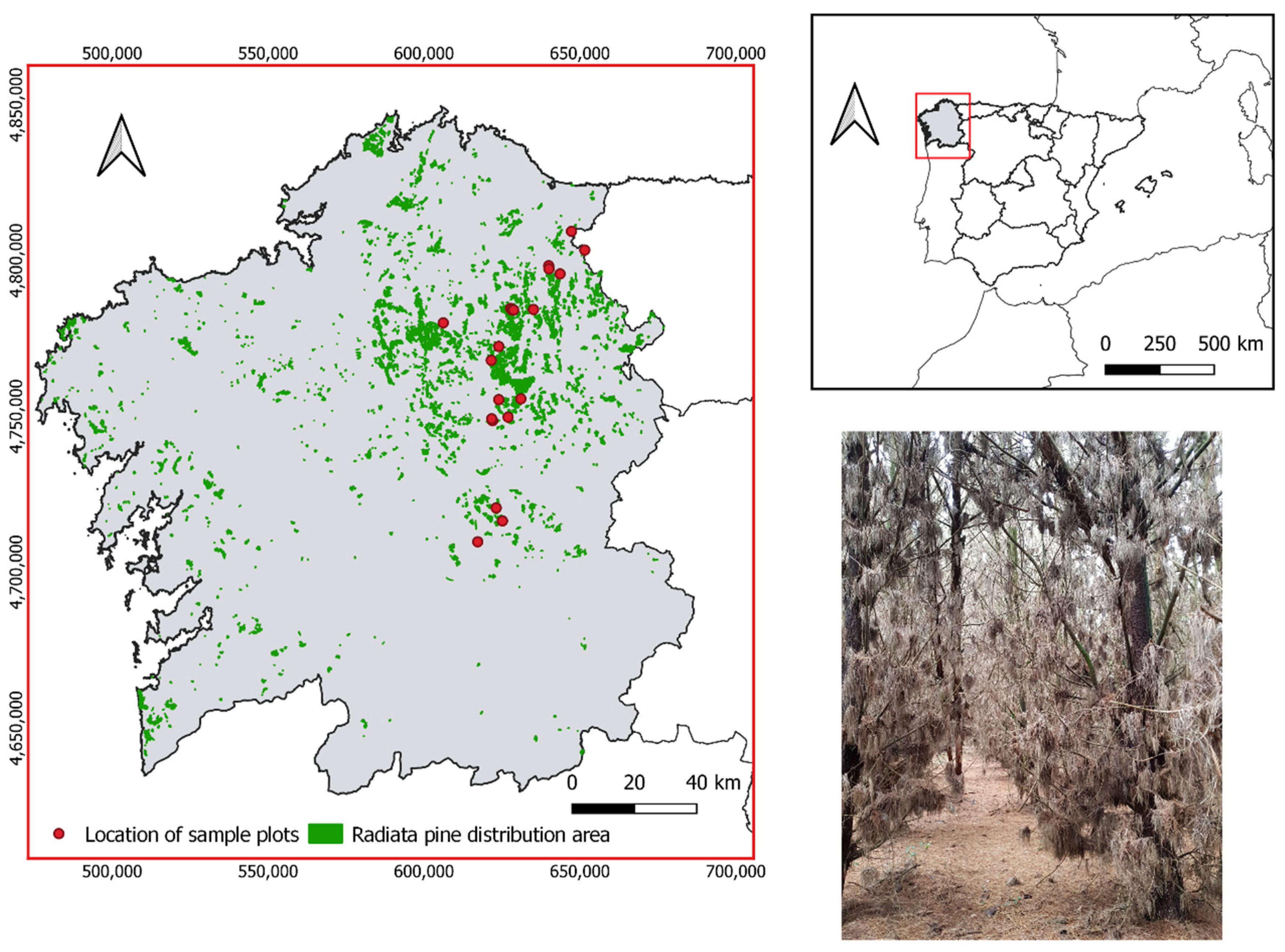
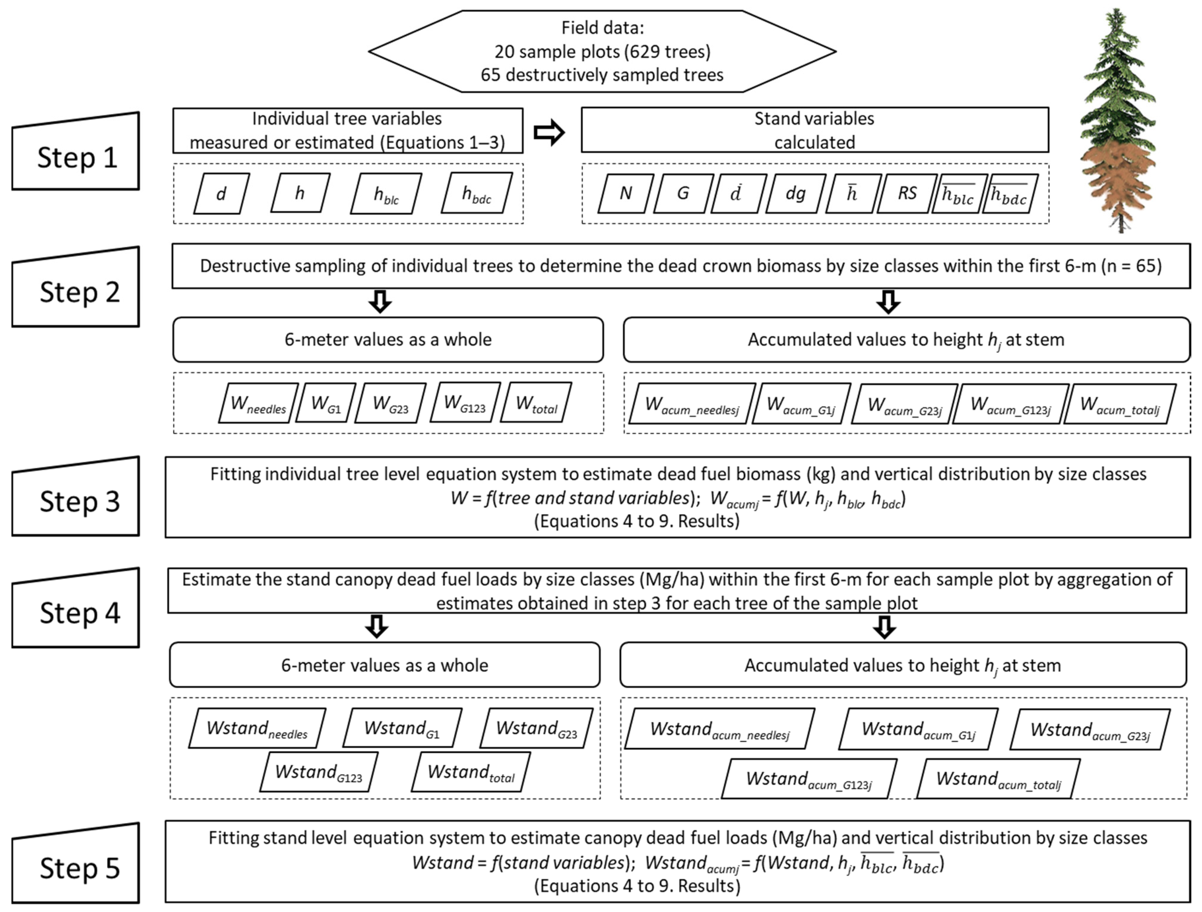
2. Materials and Methods

A total of 20 mature, pure even-aged, unmanaged stands of Pinus radiata (Figure 1) were subjectively selected to cover the observed variability in site quality and density in the area of distribution of the species in Galicia.

A temporary circular sample plot with a 10 m radius was established in each stand. The diameter at breast height (d) of all trees within the sample plot was measured to the nearest 0.1 cm at two perpendicular angles with a graduated caliper. The total tree height (h), height to the live crown base (h_blc), and height to the dead crown base (h_bdc), which were defined as the lower insertion point of respectively live branches and dead branches in a tree, were measured to the nearest 0.1 m with a digital hypsometer in a random subsample of one-third of the total trees in the sample plot (237 trees). The number of stems per hectare (N), stand basal area (G), mean diameter ($\overline{d}$), quadratic mean diameter (dg), mean stand height ($\overline{h}$), and a modification of the relative spacing index (RS), defined as $100/\left(\sqrt{N}·\overline{h}\right),$ were calculated for each sample plot from tree measurements. The dominant height, which was defined as the average height of the 100 thickest trees per ha, was not considered in this study; due to the size of the sample plots (314 m²), its value was estimated from the 4 thickest trees in the plot and would have been affected by any measurement error.

The values of h, h_blc, and h_bdc for the remaining trees in the plots were estimated by fitting a system of three equations with the measurements of the 237 subsampled trees. The system was fitted simultaneously using the iterative seemingly unrelated regression (ITSUR) method in the MODEL procedure of SAS/ETS [41]. The fitted equations explained 78%, 64%, and 98% of the observed variability in h, h_blc, and h_bdc, respectively; the following final expression, root-mean-square error (RMSE), and standard deviation of the parameter estimates (SE) were obtained as:

$$\begin{array}{c}h={\left({1.3}^{a_0}+\left({\overline{h}}^{a_0}-{1.3}^{a_0}\right)\frac{1-exp\left(-a_1·d\right)}{1-exp\left(-a_1·dg\right)}\right)}^{\raisebox{1ex}{$1$}\!\left/ \!\raisebox{-1ex}{$a_0$}\right.}RMSE=1.94 \mathrm{m}\\ a_0=1.6732 \left(SE=0.4856\right);a_1=0.0444 \left(SE=0.0197\right)\end{array}$$

(1)

$$\begin{array}{c}{h}_{blc}=h·\left(\frac{exp\left[b_0·\frac{d}{dg}+b_1·\overline{h}+b_2·G\right]}{1+exp\left[b_0·\frac{d}{dg}+b_1·\overline{h}+b_2·G\right]}\right) RMSE=2.21 \mathrm{m}\\ b_0=-0.8009 \left(SE=0.1025\right); b_1=-0.0326 \left(SE=0.0102\right); b_2=0.0306 \left(SE=0.0040\right)\end{array}$$

(2)

$$\begin{array}{c}{h}_{bdc}=h·\left(\frac{exp\left[c_0+c_1·\frac{h}{\overline{h}}+c_2·G\right]}{1+exp\left[c_0+c_1·\frac{h}{\overline{h}}+c_2·G\right]}\right) RMSE=0.18 \mathrm{m}\\ c_0=-1.9083 \left(SE=0.2600\right); c_1=-0.9932 \left(SE=0.2264\right); c_2=-0.0246 \left(SE=0.0032\right)\end{array}$$

(3)

In each plot, 2 to 4 trees in the subsample used for height measurement were subjectively selected to cover the observed diameter range. Those trees had no crown damage and branch development corresponded to the natural processes of intraspecific competition in these particular conditions. A total of 65 trees were selected and the dead crown branches within the first 6 m of the stem were destructively sampled. An upper sampling limit of 6 m was selected because this was the maximum pruning height for the species in the study area. All dead branches in each 1 m section from the base of the tree were cut and the material was bagged and taken to the laboratory, where it was physically separated into different size classes: needles, fine woody fuels (twigs diameter < 0.6 cm, hereafter G1), medium fuels (twigs 0.6 cm ≤ diameter < 2.5 cm, hereafter G2), and coarse fuels (branches 2.5 cm ≤ diameter < 7.6 cm and cones, hereafter G3). Most of the trees did not contain G3 material, so the G2 and G3 categories were grouped together (G23). Although there is no full consensus about what is considered available fuel (see [11] for clarification), for the purposes of canopy fuel modelling, only the thinnest fraction (needles and G1) is usually considered. However, fuels thicker than 6 mm were also considered in this study to enable, e.g., the total biomass contributed by dead branches for different pruning heights to be determined. Once classified, the material was weighed and dried in a forced air oven (105 °C for 24 h for fine fuels and 48 h for coarse fuels) to determine the dry biomass of each fraction (W_total, W_needles, W_G123, W_G23, and W_G1).

The compatible system of tree biomass equations developed for radiata pine in Galicia [38,42] was used to estimate the biomass of needles and fine twigs (<0.6 cm diameter) in the live crown of all trees in the plot. Three structural canopy fuel variables were then estimated using the ‘load over depth’ method: canopy fuel load (CFL), canopy base height (CBH), and canopy bulk density (CBD). CBH was calculated as the mean value of the height to the base of live crown per plot; CFL was calculated as the biomass of needles and fine twigs for all trees in the plot, which were assumed to be the fuel consumed within the flaming front of a crown fire divided by the surface plot; and CBD was calculated by dividing CFL by crown length, which was estimated as the difference between the mean stand height ($\overline{h}$) and CBH. The mean value and standard deviation for the main stand and tree variables are shown in

Table 1. Statistics for the main tree and stand variables.

Stand variables (n = 20)
Variable	Mean	Maximum	Minimum	Std. Dev.
N (stems/ha)	985.03	1368.73	604.79	222.62
G (m2/ha)	39.34	60.51	25.06	9.87
$\overline{d}$ (cm)	21.47	29.24	16.94	3.26
$\overline{h}$ (m)	19.56	25.57	14.19	3.15
RS	0.17	0.24	0.12	0.03
Live canopy variables (n = 20)
Variable	Mean	Maximum	Minimum	Std. Dev.
CBH (m)	8.64	14.09	4.65	2.80
CFL (kg/m2)	1.19	1.78	0.75	0.28
CBD (kg/m3)	0.11	0.20	0.07	0.04
Tree variables (n = 629)
Variable	Mean	Maximum	Minimum	Std. Dev.
d (cm)	21.05	49.8	4.8	8.04
h (m)	19.77	30.4	9.9	4.17
hblc (m)	8.79	19.3	2.5	3.27
hbdc (m)	0.39	1.1	0.1	0.18
Dead crown biomass within the first 6 m of destructively sampled trees (n = 65)
Variable	Mean	Maximum	Minimum	Std. Dev.
Wtotal (kg)	19.06	63.92	3.12	11.68
Wneedles (kg)	3.17	11.55	0.22	2.19
WG1 (kg)	2.10	7.55	0.31	1.09
WG23 (kg)	13.79	47.06	1.82	9.41

Std. Dev = standard deviation; N = stem density; G = stand basal area; $\overline{d}$ = mean diameter; $\overline{h}$ = mean height; RS = relative spacing index; CBH = canopy base height; CFL = canopy fuel load; CBD = canopy bulk density; d = tree diameter; h = tree height; h_blc = height to the live crown base; h_bdc = height to the dead crown base; and W_total, W_needles, W_G23, and W_G1 = total, needles, medium and coarse (G23), and woody fine (G1) fuel biomass, respectively.

.

2.1. Fuel Biomass Equations for the First 6 m of the Stem at Tree Level

Equations for estimating the biomass of each of the five fuel fractions were developed (W_total, W_needles, W_G123, W_G23, and W_G1) for the first 6 m of the stem using allometric models of the form $\widehat{W_i}={\beta }_0·X_i^{{\beta }_i}$, where $\widehat{W_i}$ is the fuel biomass of fraction i, X_i is a set of independent variables, and β₀ and β_i are parameters to be estimated. The fitted equations had to fulfil the property of additivity; i.e., the sum of biomass estimates from separate fractions had to equal the biomass estimates from the total biomass model (e.g., W_needles + W_G123 estimates had to equal W_total estimates or W_G23 + W_G1 estimates had to equal W_G123 estimates). Therefore, the equation for each fuel fraction was fitted separately in a first step and the complete system of five equations (one per fraction) was then fitted simultaneously to guarantee additivity. The best set of independent variables was selected by using the stepwise selection method after linearizing the allometric models by applying logarithmic transformations to both sides of the equation.

The equation for estimating total fuel biomass $\widehat{W_{total}}$ is expressed as follows:

$$\widehat{W_{total}}=a_0·X_i^{a_i}$$

(4)

Two equations discriminating between branch and cone biomass (W_G123) and needle biomass (W_needles) were obtained by disaggregating Equation (4):

$$\widehat{W_{needles}}=exp\left[b_{0\_n}+b_{i\_n}·log\left(X_i\right)\right]$$

$$\widehat{W_{G123}}=exp\left[b_{0\_G123}+b_{i\_G123}·log\left(X_i\right)\right]$$

$$\frac{\widehat{W_{G123}}}{\widehat{W_{total}}}=\frac{\widehat{W_{G123}}}{\left(\widehat{W_{G123}}+\widehat{W_{needles}}\right)}=\frac{1}{1+\left(\widehat{W_{needles}}/\widehat{W_{G123}}\right)}$$

The equation for estimating the branch and cone fuel biomass was then obtained as follows:

$$\widehat{W_{G123}}=\widehat{W_{total}·}\frac{1}{1+exp\left[b_0+b_i·log\left(X_i\right)\right]}$$

(5)

where b_j = b_{j_n} − b_{j_G123}; the equation to estimate the needles fuel biomass was expressed as follows:

$$\widehat{W_{needles}}=\widehat{W_{total}}-\widehat{W_{G123}}=\widehat{W_{total}}·\left[\frac{exp\left[b_0+b_i·log\left(X_i\right)\right]}{1+exp\left[b_0+b_i·log\left(X_i\right)\right]}\right]$$

(6)

Two equations for discriminating between coarse branch and cone biomass (W_G23) and fine branch biomass (W_G1) were derived by disaggregating Equation (5):

$$\widehat{W_{G23}}=exp\left[c_{0\_G23}+c_{i\_G23}·log\left(X_i\right)\right]$$

$$\widehat{W_{G1}}=exp\left[c_{0\_G1}+c_{i\_G1}·log\left(X_i\right)\right]$$

$$\frac{\widehat{W_{G23}}}{\widehat{W_{G123}}}=\frac{\widehat{W_{G23}}}{\left(\widehat{W_{G23}}+\widehat{W_{G1}}\right)}=\frac{1}{1+\left(\widehat{W_{G1}}/\widehat{W_{G23}}\right)}$$

The equation for estimating the fine dead fuel biomass was then obtained as follows:

$$\widehat{W_{G23}}=\widehat{W_{G123}·}\frac{1}{1+exp\left[c_0+c_i·log\left(X_i\right)\right]}$$

(7)

where c_j = c_{j_G1} − c_{j_G23}; the equation for estimating the live fine fuel biomass was expressed as follows:

$$\widehat{W_{G1}}=\widehat{W_{G123}}-\widehat{W_{G23}}=\widehat{W_{G123}}·\left[\frac{exp\left[c_0+c_i·log\left(X_i\right)\right]}{1+exp\left[c_0+c_i·log\left(X_i\right)\right]}\right]$$

(8)

2.2. Vertical Fuel Biomass Distribution by Height in the First 6 m of the Stem at Tree Level

The 2-parameter Weibull probability density function (PDF) was selected to describe vertical fuel biomass distribution according to height along the first 6 m of the stem for each fuel fraction:

$$W_{acum\_ij}=W_i·\left[1-exp\left(-{\left(\frac{x_j}{p_{1i}}\right)}^{p_{2i}}\right)\right], \mathrm{with} x_j=\frac{h_j-h_{bdc}}{\min \left(6,h_{blc}\right)-h_{bdc}}$$

(9)

where W_{acum_ij} is the cumulative fuel biomass of the fraction i (W_total, W_needles, W_G123, W_G23, and W_G1) at height h_j within the first 6 m of the stem; W_i is the entire 6 m stem’s fuel biomass of fraction i; h_bdc and h_blc are the dead crown base height and the live crown base height, respectively; and p₁ and p₂ are the scale and shape parameters of the 2-parameter Weibull PDF, respectively.

To ensure additivity between fractions, the W_{acum_G1j}, W_{acum_G23j}, and W_{acum_needlesj} equations were fitted so that the other fuel biomass classes (W_{acum_G123j} and W_{acum_totalj}) were estimated as the sum of the fitted fraction estimates.

2.3. Fuel Loads and Vertical Distribution in the First 6-m Layer above Ground at Stand Level

After developing the system of 8 equations for estimating fuel biomass and vertical distribution in the first 6 m of the stem of a specific tree, the equations were applied to all trees measured in each of the 20 sample plots. Thus, the fuel loads of each fraction and their vertical distribution in a 6 m layer above ground were estimated for the entire stand (Mg/ha). Finally, we used these estimates to fit a new system of 8 equations similar to that fitted for individual trees but now for entire stands.

The workflow for fitting the equation systems at individual tree and stand levels is shown in Figure 2, which provides a simple overview of the procedure described in detail in the above sections.

2.4. Statistical Analysis

The condition number was used to evaluate the presence of multicollinearity among variables in the equations fitted. According to Myers [43], condition numbers higher than $\sqrt{1000}$ indicate severe multicollinearity. The presence of heteroscedasticity was analysed by using the White test [44] and by visual inspection of Studentised residuals plotted against fitted values. In case of the presence of heteroscedasticity, each observation was weighted by the inverse of its estimated variance (${\widehat{\sigma }}_i^2$) under the assumption that this variance could be modelled as a power function of the independent variables [45]; i.e., ${\widehat{\sigma }}_i^2={\left(X_i\right)}^{exp}$. The value of the exponential term (exp) was optimised to provide the most homogeneous Studentised residual plot by using the method of Harvey [46].

As the database contained multiple equidistant observations (1 m) for each tree or stand along the 6 m layer above ground, it was reasonable to expect autocorrelation within the residuals of each tree or stand. To overcome potential autocorrelation, an autoregressive error structure of order 1 (AR1) was added to the equations to estimate the vertical distribution of fuel loads. The Durbin–Watson test was used to evaluate the possible presence of autocorrelation.

Each of the systems of 8 equations for the respective individual tree level and stand level, both of which consisted of five allometric equations for the entire 6 m layer above ground and three vertical height distribution models along the 6 m layer, were fitted simultaneously using the MODEL procedure of SAS/ETS^® [41]. In order to take cross-equation correlations into account, the ITSUR method was used to fit the system using the cross-equation error covariance matrix obtained by ordinary least squares to initiate the iterative procedure.

The database used to fit the three vertical distribution models according to height for individual trees included k measurements for each tree with a maximum of k = 6, which corresponded to the fuel loads of each fraction at heights from 1 to 6 m above ground or up to the beginning of the live crown. However, there was only one observation of W_total, W_needles, W_G123, W_G23, and W_G1 per individual tree for fitting Equations (4)–(8). As simultaneous fitting required the same number of observations for each equation in the system, the W_total, W_needles, W_G123, W_G23, and W_G1 observations were repeated k times for each tree so that those values in the simultaneous fitting were weighted by the inverse of the number of observations 1/k. The same procedure was used to fit the equations system at the stand level; e.g., [47,48].

Two goodness-of fit statistics were used to check the accuracy of estimates: model efficiency (EF) [49] and the root-mean-square error (RMSE):

$$EF=1-\frac{{\sum }_{i=1}^n{\left(Y_i-{\widehat{Y}}_i\right)}^2}{{\sum }_{i=1}^n{\left(Y_i-\overline{Y}\right)}^2}$$

(10)

$$RMSE=\sqrt{\frac{{\sum }_{i=1}^n{\left(Y_i-{\widehat{Y}}_i\right)}^2}{n-1}}$$

(11)

where $Y_i,{\widehat{Y}}_i$, and $\overline{Y}$ are the measured, estimated, and mean values of the dependent variable, respectively; and n is the total number of observations used to fit the equation.

3. Results

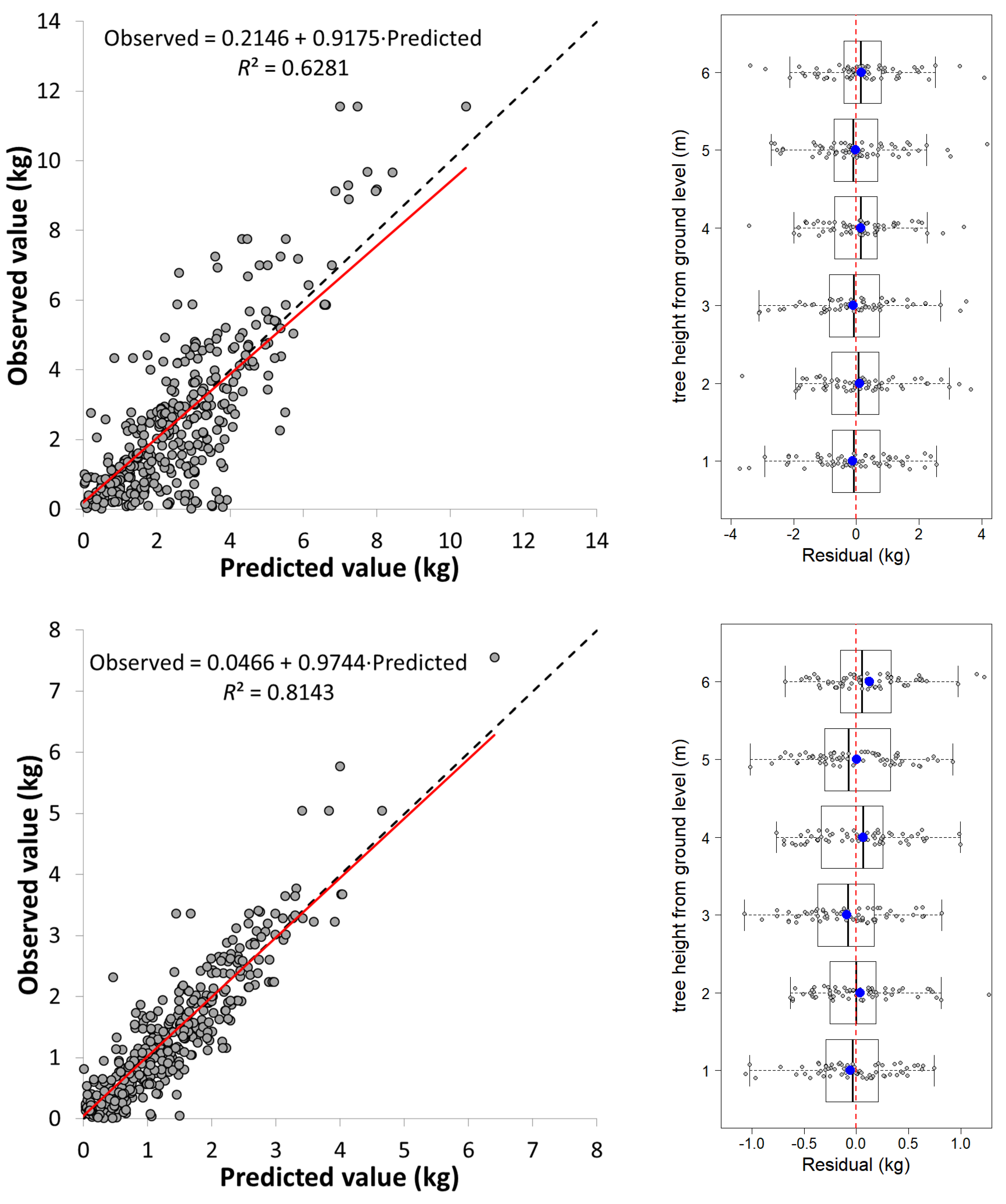
3.1. Fuel Biomass Equations and Vertical Distribution within the 6 m above the Ground Layer at the Tree Level

Once the best set of independent variables was selected for each of the five fuel biomass estimation equations (Equations (4)–(8)) for the total of the first 6 m in the stem, the entire system of eight equations was fitted simultaneously. The autoregressive terms were not initially included; however, the results of the Durbin–Watson test indicated the presence of autocorrelation in several of the vertical profile equations, so the fit was repeated. After including the AR1 term, no autocorrelation was detected.

As previously mentioned, the estimates of W_{acum_G123j} and W_{acum_totalj} were obtained as the sum of the W_{acum_G23j} + W_{acum_G1j} and W_{acum_G123j} + W_{acum_needlesj} fitted fraction estimates, respectively, and the R² and RMSE for these two individual tree fractions were then calculated.

The results of the fit of the system of equations and the values of the goodness-of-fit statistics are shown in

Table 2. System of 8 equations fitted to estimate dead fuel biomass and vertical distribution according to fuel fractions for individual trees.

Fuel Biomass Equations	Equations for Vertical Fuel Biomass Distribution
${\begin{array}{c}{W}_{total}=a_0·d^{a_1}·h_{bdc}{}^{a_2}\\ a_0=0.0222 \left(0.0084 \right); a_0=1.9745 \left(0.1046\right); a_0=-0.6329 \left(0.0711\right)\\ EF=0.5676 RMSE=7.92 \mathrm{kg}\end{array}}_{ }$	$\begin{array}{c}{W}_{acum\_totalj}=W_{acum\_G123j}+W_{acum\_needlesj}\\ EF=0.7763 RMSE=5.02 \mathrm{kg}\end{array}$
$\begin{array}{c}{W}_{G123}=\frac{W_{total}}{1+exp\left(b_0+b_1·h+b_2·\overline{h_{bdc}}+b_3·\overline{h_{blc}}\right)}\\ b_0=-1.8248 \left(0.2049\right);b_1=-0.0792 \left(0.0098\right);b_2=2.6755 \left(0.2391\right);b_3=0.0733 \left(0.0132\right)\\ EF=0.5953 RMSE=6.68 \mathrm{kg}\end{array}$	$\begin{array}{c}{W}_{acum\_G123j}=W_{acum\_G23j}+W_{acum\_G1j}\\ EF=0.7901 RMSE=4.13 \mathrm{kg}\end{array}$
$\begin{array}{c}{W}_{needles}=\frac{W_{total}·exp\left(b_0+b_1·h+b_2·\overline{h_{bdc}}+b_3·\overline{h_{blc}}\right)}{1+exp\left(b_0+b_1·h+b_2·\overline{h_{bdc}}+b_3·\overline{h_{blc}}\right)}\\ b_0=-1.8248 \left(0.2049\right);b_1=-0.0792 \left(0.0098\right);b_2=2.6755 \left(0.2391\right);b_3=0.0733 \left(0.0132\right)\\ EF=0.3530 RMSE=1.89 \mathrm{kg}\end{array}$	$\begin{array}{c}{W}_{acum\_needlesj}=W_{needles}\left[1-exp\left(-{\left(\frac{x_i}{p_{1\_needles}}\right)}^{p_{2\_Gneedles}}\right)\right]\\ p_{1\_needles}=0.3884 \left(0.0507\right); p_{2\_needles}=1.44 \left(0.10\right)\\ EF=0.6220 RMSE=1.35 \mathrm{kg}\end{array}$
$\begin{array}{c}{W}_{G23}=\frac{W_{G123}}{1+exp\left(c_0+c_1·d+c_2·RS+c_3·h_{bdc}+c_4·\frac{l_{dc}}{h}\right)}\\ c_0=-1.8878 \left(0.18\right);c_1=-0.0413\left(0.004\right);c_2=5.536 \left(0.54\right);c_3=0.9344 \left(0.16\right); c_4=-0.7637\left(0.18\right)\\ EF=0.5927 RMSE=6.15 \mathrm{kg}\end{array}$	$\begin{array}{c}{W}_{acum\_G23j}=W_{G23}\left[1-exp\left(-{\left(\frac{x_i}{p_{1\_G23}}\right)}^{p_{2\_G23}}\right)\right]\\ p_{1\_G23}=0.5612 \left(0.0305\right); p_{2\_G23}=1.87 \left(0.15\right)\\ EF=0.7805 RMSE=3.81 \mathrm{kg}\end{array}$
$\begin{array}{c}{W}_{G1}=\frac{W_{G123}·exp\left(c_0+c_1·d+c_2·RS+c_3·h_{bdc}+c_4·\frac{l_{dc}}{h}\right)}{1+exp\left(c_0+c_1·d+c_2·RS+c_3·h_{bdc}+c_4·\frac{l_{dc}}{h}\right)}\\ c_0=-1.8878 \left(0.18\right);c_1=-0.0413\left(0.004\right);c_2=5.536 \left(0.54\right);c_3=0.9344 \left(0.16\right); c_4=-0.7637\left(0.18\right)\\ EF=0.5826 RMSE=0.73 \mathrm{kg}\end{array}$	$\begin{array}{c}{W}_{acum\_G1j}=W_{G1}\left[1-exp\left(-{\left(\frac{x_i}{p_{1\_G1}}\right)}^{p_{2\_G1}}\right)\right]\\ p_{1\_G1}=0.5365 \left(0.0234\right); p_{2\_G1}=1.71 \left(0.25\right)\\ EF=0.8128 RMSE=0.46 \mathrm{kg}\end{array}$

W = dead fuel biomass (kg); d = tree diameter (cm); h = tree height (m); h_blc = height to the live crown base (m); h_bdc = height to the dead crown base (m); $\overline{h_{bdc}}$ = mean h_bdc of the stand; $\overline{h_{blc}}$ = mean h_blc of the stand; RS = relative spacing index; l_dc = length of the dead crown (h_blc -h_bdc); W_{acum_j} = accumulated dead fuel biomass to height h_j on the stem (kg) with max(h_j) = 6 and $x_i=\left(h_j-h_{bdc}\right)/\left(\min \left(6;h_{blc}\right)-h_{bdc}\right)$. Standard errors of parameter estimates are in brackets.

. All of the parameters included were significant (α = 0.05) and the values of the condition number associated with each independent variable and the results of White’s test did not indicate the presence of multicollinearity or heteroscedasticity, respectively.

The fuel biomass models explained between 35% and 59% of the observed variability in the needle fuel biomass (W_needles) and total woody and coarse fuel biomass (W_G123 and W_G23) equations, respectively, with RMSE values ranging from 0.73 kg for fine woody fuels (W_G1) to 7.92 kg for total fuel (W_total). On the other hand, the cumulative fuel biomass models to a certain height in the stem (h_j) explained between 62% (W_{acum_needlesj}) and 81% (W_{acum_G1j}) of the total observed variability, with RMSE values ranging from 0.46 kg for the fine woody fuel biomass equation (W_{acum_G1j}) to 5.02 kg for the total fuel biomass equation (W_{acum_totalj}).

By way of example, Figure 3 shows the observed versus predicted values for needles (W_{acum_needlesj}), woody fines (W_{acum_G1j}), and total (W_{acum_totalj}) fuel loads as well as the vertical distribution of the residuals of these estimates for the same fractions and sections.

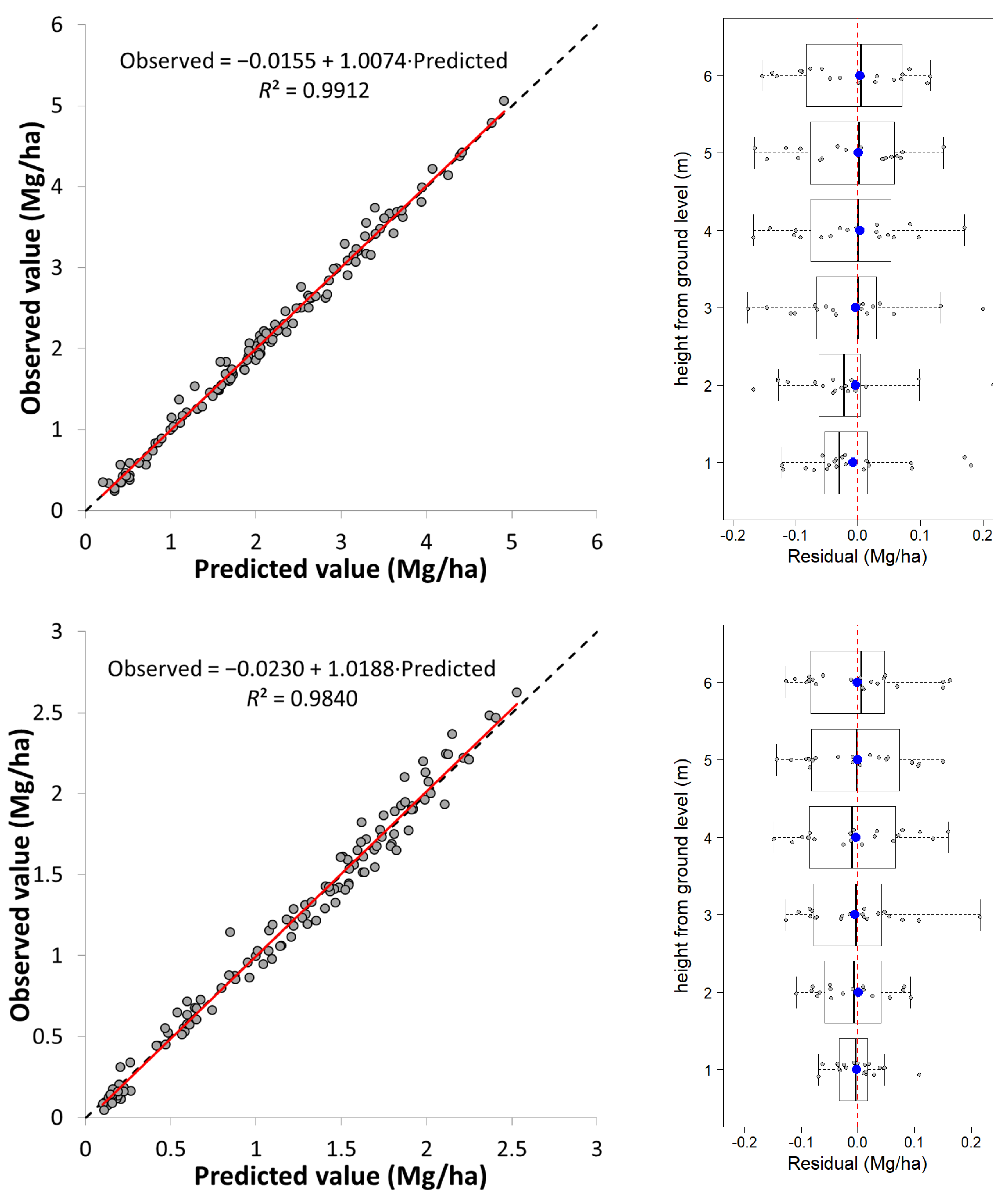
3.2. Fuel Load Equations and Vertical Distribution in the First 6 m Layer above Ground at Stand Level

Once the tree-level equations were fitted, they were applied to all the trees in each sample plot and the dead biomass values per hectare of the different fractions for the first 6 m of height from the ground were obtained by aggregating the values for each tree (

Table 3. Statistics for the main variables in the first 6 m of dead canopy and the entire canopy.

Variables for the First 6 m of Dead Canopy (n = 20)
Variable	Mean	Maximum	Minimum	Std. Dev.
Wstand_total (Mg/ha)	19.58	34.77	9.86	6.78
Wstand_needles (Mg/ha)	2.97	5.06	1.68	0.93
Wstand_G1 (Mg/ha)	1.94	2.62	1.15	0.35
Wstand_G23 (Mg/ha)	14.67	27.51	5.31	0.61
$\overline{h_{bdc}}$(m)	0.41	0.83	0.24	0.14
CFL_dead (kg/m2)	0.49	0.73	0.34	0.10
% CFL_dead	29.49	36.03	22.35	3.23
Variable for the entire canopy (dead + live) (n = 20)
Variable	Mean	Maximum	Minimum	Std. Dev.
CFL_total (kg/m2)	1.68	2.51	1.09	0.36

Std. Dev = standard deviation; Wstand__total, Wstand__needles, Wstand__G1, and Wstand__G23 = total, needles, fine woody (G1), and medium and coarse (G23) fuel load in the first 6 m of dead canopy, respectively; $\overline{h_{bdc}}$ = mean dead canopy base height in the stand; CFL__dead = available canopy fuel load of the first 6 m of dead canopy (needles + G1); %CFL__dead = percentage of CFL_{_dead} over CFL of the entire canopy (CFL__total).

).

As in the system for the individual tree, once the best set of independent variables was selected, the system of eight equations was fitted simultaneously (initially without including the autoregressive terms). In view of the results of the Durbin–Watson test, the system was refitted by including the order 1 autoregressive term (AR1). Multicollinearity and heteroscedasticity were not detected in any of the eight equations fitted. The models finally obtained, as well as the goodness-of-fit statistics, are shown in

Table 4. System of 8 equations fitted simultaneously to estimate dead fuel loads and their vertical distribution according to fuel fraction at stand level.

Fuel Load Equations	Equations for Vertical Fuel Load Distribution
${\begin{array}{c}Wstan{d}_{\_total}=a_0·G^{a_1}·{\overline{h_{bdc}}}^{a_2}\\ a_0=0.2303 \left(0.0119\right);a_1=1.1311\left(0.0142\right);a_2=-0.2993 \left(0.0148\right)\\ EF=0.9780 RMSE=1.01 \mathrm{Mg}/\mathrm{ha}\end{array}}_{}$	$\begin{array}{c}Wstan{d}_{acum\_totalj}=Wstan{d}_{acum\_needlesj}+Wstan{d}_{acum\_G123j}\\ EF=0.9909 RMSE=0.75 \mathrm{Mg}/\mathrm{ha}\end{array}$
$\begin{array}{c}Wstan{d}_{\_G123}=\frac{Wstan{d}_{\_total}}{1+exp\left(b_0+b_1·\overline{h_{bdc}}+b_2·\left(\overline{h}-\overline{h_{blc}}\right)\right)}\\ b_0=-1.8633 \left(0.0156\right); b_1=2.3581 \left(0.0259\right); b_2=-0.0740 \left(0.0011\right)\\ EF=0.9794 RMSE=0.90 \mathrm{Mg}/\mathrm{ha}\end{array}$	$\begin{array}{c}Wstan{d}_{acum\_G123j}=Wstan{d}_{acum\_G1j}+Wstan{d}_{acum\_G23j}\\ EF=0.9911 RMSE=0.67 \mathrm{Mg}/\mathrm{ha}\end{array}$
$\begin{array}{c}Wstan{d}_{\_needles}=\frac{Wstan{d}_{\_total}·exp(b_0+b_1·\overline{h_{bdc}}+b_2·\left(\overline{h}-\overline{h_{blc}}\right)}{1+exp\left(b_0+b_1·\overline{h_{bdc}}+b_2·\left(\overline{h}-\overline{h_{blc}}\right)\right)}\\ b_0=-1.8633 \left(0.0156\right); b_1=2.3581 \left(0.0259\right); b_2=-0.0740 \left(0.0011\right)\\ EF=0.9771 RMSE=0.14 \mathrm{Mg}/\mathrm{ha}\end{array}$	$\begin{array}{c}Wstan{d}_{acum\_needlesj}=Wstan{d}_{\_needles}\left[1-exp\left(-{\left(\frac{x_i}{p_{1\_needles}}\right)}^{p_{2\_needles}}\right)\right]\\ p_{1\_needles}=0.4005 \left(0.0021\right); p_{2\_needles}=1.58 \left(0.02\right)\\ EF=0.9912 RMSE=0.11 \mathrm{Mg}/\mathrm{ha}\end{array}$
$\begin{array}{c}Wstan{d}_{\_G23}=\frac{Wstan{d}_{\_G123}}{1+exp\left(c_0+c_1·G+c_2·\overline{h}\right)}\\ c_0=-0.4127 \left(0.0201\right); c_1=-0.0226 \left(0.0005\right); c_2=-0.0342 \left(0.0015\right)\\ EF=0.9819 RMSE=0.82 \mathrm{Mg}/\mathrm{ha}\end{array}$	$\begin{array}{c}{Wstan}_{d_{acum\_G23j}}=Wstan{d}_{\_G23}\left[1-exp\left(-{\left(\frac{x_i}{p_{1\_G123}}\right)}^{p_{2\_G123}}\right)\right]\\ p_{1\_G23}=0.5564 \left(0.0033\right); p_{2\_G23}=2.06 \left(0.03\right)\\ EF=0.9911 RMSE=0.61 \mathrm{Mg}/\mathrm{ha}\end{array}$
$\begin{array}{c}Wstan{d}_{\_G1}=\frac{Wstan{d}_{\_G123}·exp\left(c_0+c_1·G+c_2·\overline{h}\right)}{1+exp\left(c_0+c_1·G+c_2·\overline{h}\right)}\\ c_0=-0.4127 \left(0.0201\right); c_1=-0.0226 \left(0.0005\right); c_2=-0.0342 \left(0.0015\right)\\ EF=0.8829 RMSE=0.12 \mathrm{Mg}/\mathrm{ha}\end{array}$	$\begin{array}{c}{Wstan}_{d_{acum\_G1j}}=Wstan{d}_{\_G1}\left[1-exp\left(-{\left(\frac{x_i}{p_{1\_G1}}\right)}^{p_{2\_G1}}\right)\right]\\ p_{1\_G1}=0.5280 \left(0.0036\right); p_{2\_G1}=1.90 \left(0.03\right)\\ EF=0.9837 RMSE=0.09 \mathrm{Mg}/\mathrm{ha}\end{array}$

Wstand = fuel load (Mg/ha); h_blc = height to the base of the live crown (m); h_bdc = height to the dead crown base (m); $\overline{h_{bdc}}$ = mean h_bdc of the stand; $\overline{h_{blc}}$ = mean h_blc of the stand; $\overline{h}$ = mean height of the stand; G = stand basal area; Wstand__{acum_j} = accumulated dead fuel load to height h_j in the stem (Mg/ha) with max(h_j) = 6 and $x_i=\left(h_j-\overline{h_{bdc}}\right)/\left(\min \left(6,\overline{h_{blc}}\right)-\overline{h_{bdc}}\right)$. Standard errors of parameter estimates are in brackets.

. All parameters included in the models were significant (α = 0.05).

Again, once the eight equations were fitted, the Wstand_{acum_G123j} and Wstand_{acum_totalj} values for each stand were estimated as the sum of the Wstand_{acum_G23j} + Wstand_{acum_G1j} and Wstand_{acum_G123j} + Wstand_{acum_needlesj} estimates, respectively. The R² and RMSE values were then calculated for these two fractions.

The fuel load models explained between 88% and 98% of the observed variability in the fine woody fuel load (Wstand__G1) and the other fuel fractions (Wstand__total, Wstand__G123, Wstand__needles, and Wstand__G23) equations, respectively. The RMSE values ranged from 0.12 Mg/ha for fine woody fuel (Wstand__G1) to 1.01 Mg/ha for total fuel load (Wstand__total). The cumulative fuel load models explained more than 98% of the total observed variability, with RMSE values ranging from 0.09 Mg/ha for the fine woody fuel load equation (Wstand_{acum_G1j}) to 0.75 Mg/ha for the total fuel load equation (Wstand_{acum_totalj}).

Figure 4 shows the observed versus predicted values for needles (Wstand_{acum_needlesj}), woody fine (Wstand_{acum_G1j}), and total (Wstand_{acum_totalj}) fuel loads as well as the vertical distribution of the residuals of these estimates for the same fractions and sections.

4. Discussion

The values of the stand variables and live-canopy structural variables (CBH, CFL, and CBD) observed in this study were within the range of values obtained for Pinus radiata in other studies conducted in the same geographic area and under similar climatic, physiographic, and edaphic conditions; e.g., [11,12,14,21]. Moreover, the observed mean values of stem density (N), stand basal area (G), mean height ($\overline{h}$), and CFL were consistent with those reported by Gomez-Vazquez et al. [14] for the same species and the mean value of CBD (0.11 kg/m³) was the same as that observed by Arellano-Pérez et al. [21] and slightly exceeded the threshold of 0.1 kg/m³ empirically deduced by Agee [50] as the approximate value necessary to support active crowning.

The mean CBH in the sample plots analysed in this study was 8.6 m (sd = 2.8 m) with a maximum of 14.1 m, whereas the mean height of dead fuel initiation was 0.4 m (sd = 0.1 m) with a maximum of 0.8 m. Thus, the dead canopy base height rather than the live height should be used to assess the potential for crown fire initiation in closed and unmanaged radiata pine stands. Consequently, a fire behaviour system based on FSG rather on CBH should be used; namely, PPPY [5] or AMICUS [39]. Users of USDA Forest Service fire behaviour modelling tools, which rely on the crown fire initiation equation in [3] that used CBH as an input, are advised to incorporate ladder fuels in the surface fuel complex as previously suggested [7,51], even if this solution is only partially satisfactory because it implies custom fuel modeling or making an adjustment to the surface fireline intensity. Regarding CFL, the mean value observed when including only the fine live canopy was 1.19 kg/m² (sd = 0.28 kg/m²) with a maximum of 1.78 kg/m²; these values increased to 1.68 kg/m² (sd = 0.36 kg/m²) and 2.51 kg/m², respectively, when adding the load provided by the needles and fine twigs of the dead branches that extended into the surface fuel layer to the fine live crown. Therefore, the important contribution of dead ladder fuel to the total available fuel load (mean and maximum values of 29.5% (sd = 3.2) and 36%, respectively, in this study) must be highlighted because it implies an increase of similar proportions in the heat per unit area released by a fire consuming all fine components. For example, according to Byram [52] and considering the usual low net heat of combustion of 18,000 kJ/kg [5,40], the energy released by the crowns would increase from 21,420 kJ/m² to 30,240 kJ/m², which represents a 41.1% increase in fireline intensity. Our findings confirmed that these pine plantations did not have a homogeneous distribution of live and dead fine fuel in the canopy, similar to their Australian counterparts [40]. Instead, two clearly different fuel layers were present: a lower layer predominantly comprising dead fuels characterised by high flammability when dry enough and an upper layer predominantly comprising live fuels with a higher bulk density.

The goodness-of-fit statistics of the two equation systems developed indicated robust and accurate estimates, so these systems contributed to filling the gap on how to quantify dead ladder fuels and improve the estimates of potential heat release per unit and fireline intensity. Although both equation systems can be used for the same purpose of estimating dead ladder fuels load according to classes and their vertical distribution in the stand, their advantages and limitations must be considered. The use of the tree-level equation systems (Table 2) requires a large number of independent variables and the calculation is more complicated than the direct use of the stand-level system (Table 4). The process involves calculating the biomass of each tree, aggregating the biomass of all trees in the sample plot, and expressing the result relative to the unit area (ha). However, despite apparently poorer goodness-of-fit statistics, the tree-level system is more accurate because it is based on actual dead fuel data obtained from destructively sampled trees whereas the stand-level system (Table 4) is based on tree biomass values estimated by the system of equations at the individual tree level (Table 2). On the other hand, the stand-level system is simpler to apply because it only required a sample of trees to obtain representative mean values rather than the measurement of the total, dead crown initiation, and live crown initiation heights of all trees in the plot.

In any case, the use of either approach will basically depend on the required balance between the accuracy of the estimates to be obtained (higher accuracy with the individual-tree approach) and the cost that can be assumed in the field inventory (lower cost with the stand approach).

5. Conclusions

Accurate characterization of the load and vertical distribution of ladder fuels is essential for forest managers given the importance of this type of fuel as a surface-to-crown-fire transition factor by providing greater vertical fuel continuity. In addition, ladder fuels in unmanaged pine stands of species characterised by poor self-pruning such as the Pinus radiata considered here can greatly hinder firefighting efforts and safety by limiting mobility and visibility due to their high density. Both systems of models fitted in this study can be used to quantify the dead ladder fuels extending to near the ground in closed-canopy and unpruned pure and even-aged P. radiata stands. This information will allow forest managers to simulate how different pruning heights up to 6 m affect potential crown-fire hazards for a range of meteorological and fuel moisture scenarios as well as for different treatment alternatives for the woody debris generated (removal, mastication, or no management). These modelling systems should be used in combination with live CFL models for radiata pine (e.g., [12]) to estimate the total load of the fine fuel fraction in this type of stand. This will prevent underestimation of the available canopy fuel load as well as overestimation of the fuel strata gap and will thus prevent errors in assessing crown fire potential activity, including onset of crowning, type of crown fire, and the associated fire behaviour characteristics (fire-spread rate and fireline intensity).

References

1. Keane, R.E. Wildland Fuel Fundamentals and Applications; Springer International Publishing: New York, NY, USA, 2015. [Google Scholar]
2. Reardon, J. Ground Fuel. In Encyclopedia of Wildfires and Wildland-Urban Interface (WUI) Fires; Manzello, S.L., Ed.; Springer: Cham, Switzerland, 2020; pp. 1–8. [Google Scholar]
3. Van Wagner, C.E. Conditions for the start and spread of crown fire. Can. J. For. Res. 1977, 7, 23–34. [Google Scholar] [CrossRef]
4. Alexander, M.E.; Cruz, M.G. Crown fire dynamics in conifer forests. In Synthesis of Knowledge of Extreme Fire Behavior: Volume I for Fire Managers; Werth, P.A., Potter, B.E., Clements, C.B., Finney, M.A., Goodrick, S.L., Alexander, M.E., Cruz, M.G., Forthofer, J.A., McAllister, S.S., Eds.; USDA, Forest Service, Pacific Northwest Research Station: Corvallis, OR, USA, 2011; Volume PNW-GTR-854, pp. 107–144. [Google Scholar]
5. Cruz, M.G.; Alexander, M.E.; Fernandes, P.M. Development of a model system to predict wildfire behaviour in pine plantations. Aust. For. 2008, 71, 113–121. [Google Scholar] [CrossRef] [Green Version]
6. Sando, R.W.; Wick, C.H. A Method of Evaluating Crown Fuels in Forest Stands; USDA, Forest Service, Res. Pap. NC-84: St. Paul, MN, USA, 1972. [Google Scholar]
7. Scott, J.H.; Reinhardt, E.D. Assessing Crown Fire Potential by Linking Models of Surface and Crown Fire Behavior; USDA Forest Service, Rocky Mountain Research Station, Res. Pap. RMRS-RP-29: Fort Collins, CO, USA, 2001. [Google Scholar]
8. Stocks, B.J.; Alexander, M.E.; Wotton, B.M.; Stefner, C.N.; Flannigan, M.D.; Taylor, S.W.; Lavoie, N.; Mason, J.A.; Hartley, G.R.; Maffey, M.E.; et al. Crown fire behaviour in a northern jack pine—Black spruce forest. Can. J. For. Res. 2004, 34, 1548–1560. [Google Scholar] [CrossRef] [Green Version]
9. Keyser, T.; Smith, F.W. Influence of crown biomass estimators and distribution on canopy fuel characteristics in ponderosa pine stands of the Black Hills. For. Sci. 2010, 56, 156–165. [Google Scholar]
10. Cruz, M.; Alexander, M. Assessing crown fire potential in coniferous forests of western North America: A critique of current approaches and recent simulation studies. Int. J. Wildland Fire 2010, 19, 377–398. [Google Scholar] [CrossRef]
11. Ruiz-González, A.D.; Álvarez-González, J.G. Canopy bulk density and canopy base height equations for assessing crown fire hazard in Pinus radiata plantations. Can. J. For. Res. 2011, 41, 839–850. [Google Scholar] [CrossRef]
12. Fernández-Alonso, J.M.; Alberdi, I.; Álvarez-González, J.G.; Vega, J.A.; Cañellas, I.; Ruiz-González, A.D. Canopy fuel characteristics in relation to crown fire potential in pine stands: Analysis, modelling and classification. Eur. J. For. Res. 2013, 132, 363–377. [Google Scholar] [CrossRef]
13. Hevia, A.; Crabiffosse, A.; Majada, J.; Álvarez-González, J.G.; Ruiz-González, A.D. Modelo de distribución de la carga de combustibles finos en el dosel de copas de rodales regulares de Pinus pinaster: Efecto de claras combinadas con podas. Cuad. La SECF 2012, 34, 123–133. [Google Scholar]
14. Gómez-Vázquez, I.; Crecente-Campo, F.; Diéguez-Aranda, U.; Castedo-Dorado, F. Modelling canopy fuel variables in Pinus pinaster Ait. and Pinus radiata D. Don stands in northwestern Spain. Ann. For. Sci. 2012, 70, 161–172. [Google Scholar] [CrossRef] [Green Version]
15. Ruiz-González, A.D.; Castedo-Dorado, F.; Vega, J.A.; Jiménez, E.; Fernández-Alonso, J.M.; Álvarez-González, J.G. Modelling canopy fuel dynamics of maritime pine stands in north-west Spain. Int. J. Wildland Fire 2015, 24, 92–102. [Google Scholar] [CrossRef]
16. Arellano-Pérez, S.; Álvarez-González, J.G.; Vega Hidalgo, J.A.; Ruiz González, A.D. Modelos de estimación de la distribución vertical de combustibles finos de copa en masas de pinar a partir de datos del IV Inventario Forestal Nacional. In Proceedings of the VII Congreso Forestal Español: “Gestión Del Monte: Servicios Ambientales y Bioeconomía”, Plasencia, Spain, 26–30 June 2017. [Google Scholar]
17. Hevia, A.; Álvarez-González, J.G.; Ruiz-Fernández, E.; Ruiz-González, A.D.; Majada, J.; González-Ferreiro, E. Modelling canopy fuel and forest stand variables and characterizing the influence of thinning in the stand structure using airborne LiDAR. Rev. Teledetección 2016, 45, 41–55. [Google Scholar] [CrossRef] [Green Version]
18. González-Ferreiro, E.; Arellano-Pérez, S.; Castedo-Dorado, F.; Hevia, A.; Vega, J.A.; Vega-Nieva, D.; Álvarez-González, J.G.; Ruiz-González, A.D. Modelling the vertical distribution of canopy fuel load using national forest inventory and low-density airbone laser scanning data. PLoS ONE 2017, 12, e0176114. [Google Scholar] [CrossRef] [PubMed]
19. Alberdi, I.; Vallejo, R.; Álvarez-González, J.G.; Condés, S.; González-Ferreiro, E.; Guerrero, S.; Hernández, L.; Martínez-Jauregui, M.; Montes, F.; Oliveira, N.; et al. The multi-objective Spanish National Forest Inventory. For. Syst. 2017, 26, e04S. [Google Scholar] [CrossRef]
20. Fidalgo-González, L.; Arellano-Pérez, S.; Castedo-Dorado, F.; Ruiz-González, A.D.; González-Ferreiro, E. Estimación de la distribución vertical de combustibles finos del dosel de copas en masas de Pinus sylvestris empleando datos LiDAR de baja densidad. Rev. Teledetección 2019, 53, 1–16. [Google Scholar] [CrossRef]
21. Arellano-Pérez, S.; Castedo-Dorado, F.; López-Sánchez, C.A.; González-Ferreiro, E.; Yang, Z.; Díaz-Varela, R.A.; Álvarez-González, J.G.; Vega, J.A.; Ruiz-González, A.D. Potential of Sentinel-2A data to model surface and canopy fuel characteristics in relation to crown fire hazard. Remote Sens. 2018, 10, 1645. [Google Scholar] [CrossRef] [Green Version]
22. Finney, M.A. An overview of FlamMap fire modeling capabilities. In Fuels Management-How to Measure Success: Conference Proceedings; Andrews, P.L., Butler, B.W., Eds.; USDA, Forest Service, Rocky Mountain Research Station: Fort Collins, CO, USA, 2006; Volume 41, pp. 213–220. [Google Scholar]
23. Cruz, M.G.; Alexander, M.E.; Wakimoto, R.H. Modeling the likelihood of crown fire occurrence in conifer forest stands. For. Sci. 2004, 50, 640–658. [Google Scholar]
24. Arellano-Pérez, S.; Vega, J.A.; Ruíz-González, A.D.; Arellano, A.; Álvarez-González, J.G.; Vega-Nieva, D.J.; Pérez, E. Foto-guía de Combustibles Forestales de Galicia y Comportamiento del Fuego Asociado; Andavira: Santiago de Compostela, Spain, 2017. [Google Scholar]
25. Vega, J.A.; Arellano-Pérez, S.; Álvarez-González, J.G.; Fernández, C.; Jiménez, E.; Fernández-Alonso, J.M.; Vega-Nieva, D.J.; Briones-Herrera, C.; Alonso-Rego, C.; Fontúrbel, T.; et al. Modelling aboveground biomass and fuel load components at stand level in shrub communities in NW Spain. For. Ecol. Manag. 2022, 505, 119926. [Google Scholar] [CrossRef]
26. Alonso-Rego, C.; Arellano-Pérez, S.; Cabo, C.; Ordoñez, C.; Álvarez-González, J.G.; Díaz-Varela, R.A.; Ruiz-González, A.D. Estimating fuel loads and structural characteristics of shrub communities by using terrestrial laser scanning. Remote Sens. 2020, 12, 3704. [Google Scholar] [CrossRef]
27. Alonso-Rego, C.; Arellano-Pérez, S.; Guerra-Hernández, J.; Molina-Valero, J.A.; Martínez-Calvo, A.; Pérez-Cruzado, C.; Castedo-Dorado, F.; González-Ferreiro, E.; Álvarez-González, J.G.; Ruiz-González, A.D. Estimating Stand and Fire-Related Surface and Canopy Fuel Variables in Pine Stands Using Low-Density Airborne and Single-Scan Terrestrial Laser Scanning Data. Remote Sens. 2021, 13, 5170. [Google Scholar] [CrossRef]
28. Vega, J.A. Efectos del Fuego Prescrito Sobre el Suelo en Pinares de Pinus pinaster Ait. de Galicia. Ph.D. Thesis, Universidad Politécnica de Madrid, Madrid, Spain, 2001. [Google Scholar]
29. Fernandes, P.M.; Rigolot, E. The fire ecology and management of maritime pine (Pinus pinaster Ait.). For. Ecol. Manag. 2007, 241, 1–13. [Google Scholar] [CrossRef]
30. MARM. Cuarto Inventario Forestal Nacional. Galicia; Ministerio de Medio Ambiente y Medio Rural y Marino: Madrid, Spain, 2011. [Google Scholar]
31. DGCN. Tercer Inventario Forestal Nacional 1997–2006: Galicia; Ministerio de Medio Ambiente: Madrid, Spain, 2000. [Google Scholar]
32. Consellería del Medio Rural. ORDEN de 9 de Febrero de 2021. Available online: https://www.xunta.gal/dog/Publicados/2021/20210226/AnuncioG0426-110221-0005_es.html (accessed on 12 April 2022).
33. Keeley, J.E.; Zedler, P.H. Evolution of life histories in Pinus. In Ecology and Biogeography of Pinus; Richardson, D.M., Ed.; Cambridge University Press: Cambridge, UK, 1998; pp. 219–250. [Google Scholar]
34. Menning, K.M.; Stephens, S.L. Fire climbing in the forest: A semiqualitative, semiquantitative approach to assessing ladder fuel hazards. West. J. Appl. For. 2007, 22, 88–93. [Google Scholar] [CrossRef] [Green Version]
35. Hirsch, K.; Martell, D. A review of initial attack fire crew productivity and effectiveness. Int. J. Wildland Fire 1996, 6, 199–215. [Google Scholar] [CrossRef]
36. Kramer, H.A.; Collins, B.M.; Lake, F.K.; Jakubowski, M.K.; Stephens, S.L.; Kelly, M. Estimating ladder fuels: A new approach combining field photography with LiDAR. Remote Sens. 2016, 8, 766. [Google Scholar] [CrossRef]
37. Norgaard, K.M. The Politics of fire and the social impacts of fire exclusion on the Klamath. Humboldt J. Soc. Relat. 2014, 36, 77–101. [Google Scholar]
38. Balboa-Murias, M.A.; Rodríguez-Soalleiro, R.; Merino, A.; Álvarez-González, J.G. Temporal variations and distribution of carbon stocks in aboveground biomass of radiata pine and maritime pine pure stands under different silvicultural alternatives. For. Ecol. Manag. 2006, 237, 29–38. [Google Scholar] [CrossRef]
39. Plucinski, M.P.; Sullivan, A.L.; Rucinski, C.J.; Prakash, M. Improving the reliability and utility of operational bushfire behaviour predictions in australian vegetation. Environ. Model Softw. 2017, 91, 1–12. [Google Scholar] [CrossRef]
40. Cruz, M.G.; Alexander, M.E.; Plucinski, M.P. The effect of silvicultural treatments on fire behaviour potential in radiata pine plantations of South Australia. For. Ecol. Manag. 2017, 397, 27–38. [Google Scholar] [CrossRef]
41. SAS Institute Inc. SAS/ETS® 9.1 User’s Guide; SAS Institute Inc.: Cary, NC, USA, 2004. [Google Scholar]
42. Dieguez-Aranda, U.; Rojo-Alboreca, A.; Castedo-Dorado, F.; Álvarez-González, J.G.; Barrio-Anta, M.; Crecente-Campo, F.; González-González, J.M.; Pérez-Cruzado, C.; Rodriguez-Soalleiro, R.; López-Sánchez, C.A.; et al. Herramientas Selvícolas para la Gestión Forestal Sostenible en Galicia; Consellería do Medio Rural, Xunta de Galicia: Santiago de Compostela, Spain, 2009. [Google Scholar]
43. Myers, R.H. Classical and Modern Regression with Applications, 2nd ed.; Duxbury Press: Belmont, CA, USA, 1990. [Google Scholar]
44. White, H.A. Heteroskedasticity-consistent covariance matrix estimator and a direct test for heteroskedasticity. Econometrica 1980, 48, 817–838. [Google Scholar] [CrossRef]
45. Cailliez, F. Estimación del Volumen Forestal y Predicción del Rendimiento; FAO: Rome, Italy, 1980. [Google Scholar]
46. Harvey, A.C. Estimating regression models with multiplicative heteroscedasticity. Econometrica 1976, 44, 461–465. [Google Scholar] [CrossRef]
47. Diéguez-Aranda, U.; Castedo-Dorado, F.; Álvarez-González, J.G.; Rojo, A. Compatible taper function for Scots pine plantations in northwestern Spain. Can. J. For. Res. 2006, 36, 1190–1205. [Google Scholar] [CrossRef]
48. Hevia, A.; Crabiffosse, A.; Álvarez-González, J.G.; Ruiz-González, A.D.; Majada, J. Novel approach to assessing residual biomass from pruning: A case study in Atlantic Pinus pinaster Ait. timber forests. Renew. Energ. 2017, 107, 620–628. [Google Scholar] [CrossRef]
49. Mayer, D.G.; Butler, D.G. Statistical validation. Ecol. Model. 1993, 68, 21–32. [Google Scholar] [CrossRef]
50. Agee, J.K. The influence of forest structure on fire behavior. In Proceedings of the 17th Annual Forest Vegetation Management Conference, Sacramento, CA, USA, 16–18 January 1996. [Google Scholar]
51. Hall, S.A.; Burke, I.C. Considerations for characterizing fuels as inputs for fire behavior models. For. Ecol. Manag. 2006, 227, 102–114. [Google Scholar] [CrossRef]
52. Byram, G.M. Combustion of forest fuels. In Forest Fire: Control and Use; Davis, K.P., Ed.; McGraw-Hill: New York, NY, USA, 1959; pp. 61–89. [Google Scholar]
Figure 1. Geographical location of Pinus radiata stands in Galicia and of the 20 plots included in the study (left). View of one of the study plots (lower right).
Forests 13 01697 g001
Figure 2. Workflow for fitting the equation systems at individual tree and stand levels.
Forests 13 01697 g002
Figure 3. (Left) Scatter plots of observed versus predicted values for the vertical distribution of needles (Wacum_needlesj, upper), woody fines (Wacum_G1j, middle), and total (Wacum_totalj, lower) individual tree fuel loads. The solid red line denotes the fitted linear model and the dashed line denotes perfect agreement. (Right) Box plots of the vertical distribution of residuals of needles (Wacum_needlesj, upper), woody fine (Wacum_G1j, middle), and total (Wacum_totalj, lower) individual tree fuel loads according to heights from ground level. Blue dots denote the mean values.
Forests 13 01697 g003aForests 13 01697 g003b
Figure 4. (Left) Scatter plots of observed versus predicted values for the vertical distribution of needles (Wstandacum_needlesj, upper), woody fine (Wstandacum_G1j, middle), and total (Wstandacum_totalj, lower) stand fuel loads. The solid red line denotes the fitted linear model and the dashed line denotes perfect agreement. (Right) Box plots of the vertical distribution of residuals of needles (Wstandacum_needlesj, upper), woody fines (Wstandacum_G1j, middle), and total (Wstandacum_totalj, lower) stand fuel loads according to heights from ground level. Blue dots denote the mean values.
Forests 13 01697 g004aForests 13 01697 g004b