Seemingly Unrelated Mixed-Effects Biomass Models for Black Locust in West Poland

Abstract

Information about tree biomass is important not only in the assessment of wood resources but also in the process of preparing forest management plans, as well as for estimating carbon stocks and their flow in forest ecosystems. The study aimed to develop empirical models for determining the dry mass of the aboveground parts of black locust trees and their components (stem, branches, and leaves). The research was carried out based on data collected in 13 stands (a total of 38 sample trees) of black locust located in western Poland. The model system was developed based on multivariate mixed-effect models using two approaches. In the first approach, biomass components and tree height were defined as dependent variables, while diameter at breast height was used as an independent variable. In the second approach, biomass components and diameter at breast height were dependent variables and tree height was defined as the independent variable. Both approaches enable the fixed-effect and cross-model random-effect prediction of aboveground dry biomass components of black locust. Cross-model random-effect prediction was obtained using additional measurements of two extreme trees, defined as trees characterized by the smallest and largest diameter at breast height in sample plot. This type of prediction is more precise (root mean square error for stem dry biomass for both approaches equals 77.603 and 188.139, respectively) than that of fixed-effects prediction (root mean square error for stem dry biomass for both approaches equals 238.716 and 206.933, respectively). The use of height as an independent variable increases the possibility of the practical application of the proposed solutions using remote data sources.

1. Introduction

Black locust (Robinia pseudoacacia L.) is an alien tree species in Poland. Its natural range covers the southeastern part of the United States, and its optimum elevation range is between 150 and 1500 m above sea level in the Appalachian Mountains [1]. This tree species was brought to Europe around 1600 by the French gardener Jean Robin [2]. Initially, black locust was grown mainly as a park tree. Over time, due to its properties, the species has found a wider application [2,3,4]. The mechanical properties of the black locust wood make it suitable for veneers, fence posts, poles, flooring, furniture, and boat building. It is also a source of valuable fuelwood because of its high calorific potential [4,5]. This tree species is recommended for soil restoration and regeneration of damaged habitats. Due to its low habitat requirements and ability to fix atmospheric nitrogen, it is planted on degraded, post-industrial, post-agricultural, and initial soils [6,7,8,9,10]. Black locust is now quite common in the United Kingdom, Germany, France, the Netherlands, Belgium, Italy, and Switzerland [11]. It is the most frequently planted tree species in Hungary, occupying 23% of the total forest area of the country [12]. Moreover, the distribution of black locust throughout Europe appears to be mostly limited by low temperatures, but global warming might enhance its growth in presently colder areas [13,14].

Black locust was brought to Poland in 1806 [15]. Currently, this tree species occurs almost all over the country, but most of it is found in the western part of Poland. The black locust stands occupy over 273,000 ha and provide 84,000 m³ of wood annually. In areas with a high share of this tree species, wood demand outweighs the supply [16,17].

The information about tree biomass is important not only for the assessment of wood resources, but it is also a significant element in the process of forest management plan preparation. This data is needed for the estimation of carbon stock in forest ecosystems [18]. Concerning climate change, there is a need to monitor changes in the forest carbon stock and how they influence the atmospheric CO₂ concentration. Obtaining reliable data on forest biomass and carbon stock allows to improve the estimation of the forest carbon sink and its role in the global carbon cycle as a counteraction to the global climate change [19].

The estimation of the carbon stock accumulated in the forest is difficult and requires reliable tools for its estimation. Despite the growing importance of remote sensing methods in collecting biological data about the forest (including volume, aboveground biomass, and amount of accumulated carbon, etc.), the methods based on field measurements are still important tools to assess forest resources [20] and often are used to verify the results obtained by remote sensing techniques [21].

One of the methods of assessing the tree and stand biomass is to use empirical models based on easy-to-measure tree parameters such as diameter at breast height (DBH) or height (H). Due to the high variability in the shape and structure of tree stems (observed even within one tree species) resulting from the genetically determined variability, local growing conditions, forest treatments, etc., it seems necessary to develop local models to determine the biomass of trees and their components [22,23].

The tree and stand biomass data are characterized by a grouped structure, containing information about trees and sample plot. Modeled relationships between dependent and independent variables differ among sample plots. The mixed-effects models make it possible to describe dependencies at different levels of the data [24,25]. The fixed-effects approach allows modeling data for a typical sample plot (defined grouping level), while the random-effects approach defines difference between each plot and the typical plot [26]. The description of dependencies at different levels translates into the flexibility of predictive model. If no local information is available to estimate the random effects, the prediction using the fixed part of the model can be used. In the case of sufficient data availability, a more accurate random-effects prediction can be carried out [27,28,29]. Random-effects prediction takes on a new meaning in the case of multivariate models, in which the cross-model correlations within the system of developed models based on the estimated best linear unbiased predictor (EBLUP) is used [28]. In addition, mixed-effects biomass models are fitted in different forms, as they can be nonlinear [30] or linear with logarithmic data transformation [26,27,31].

During biomass modeling, it is worth considering the logical assumption that the sum of the biomass components of the tree estimated using equations should be equal to the estimated biomass of the whole tree (so-called additivity of the biomass models). This assumption can be met by seemingly unrelated regression application [32,33]. The assumption about the additivity of the biomass model was the basis of biomass models e.g., in Germany [34], Canada [35], and Poland [36]. Above papers are examples of using the seemingly unrelated regression. However, the knowledge of the authors indicates that no research has been undertaken yet that focuses on the development of model systems using diameter at breast height and height as both independent and dependent variables.

This study aimed to develop empirical models for determining the dry mass of the aboveground part of black locust trees and its components (stem, branches, and leaves). The models were developed using multivariate mixed-effects models with sample plot as grouping level. To obtain a compatible set of models, we used a seemingly unrelated regression [32,33]. We fitted two approaches of the models. In the first one, as a classic one, DBH was the independent variable. In the second one, the H was defined as the independent variable. Second approach is a new concept to biomass modeling, which allows to increase the practical application of the proposed solutions using remote sensing data sources. Moreover, we developed the model system applying the cross-model calibration (random-effects prediction) of the biomass component models using H and DBH.

2. Materials and Methods

2.1. Study Sites

The data was collected in West Poland (two State Forest Districts with a total area equal to 50,000 ha, 52°08′–51°30′ N, 15°23′–16°14′ E), which is the region with the highest abundance of black locust in Polish forests [17]. We selected 13 stands located on oligotrophic sites that are typically occupied by the investigated species in Poland (

Table 1. Summary characteristics of the black locust sample plots located in West Poland: average stand age (A, years), stocking (N, trees ha⁻¹), basal area (BA, m² ha⁻¹), average diameter at breast height (Dg, cm), and average height (Hg, m).

	Minimum	Maximum	Mean	Median	Standard Deviation
A	16	85	50	50	21
N	167	1134	586	507	304
BA	10.06	40.52	21.73	20.53	7.72
Dg	11.47	43.94	23.94	25.23	9.08
Hg	9.84	27.19	20.30	21.18	5.19

). The chosen stands grew on moderate fertile rusty soils. The study sites are located in a transition zone from maritime temperate to continental temperate climate [37]. The mean annual temperature reaches 9.5 °C. January is the coldest month with an average temperature slightly below 0 °C, while the highest average temperature is recorded in July (+19.0 °C). The average annual precipitation is rather low and rarely exceeds 550–600 mm. The majority of the rainfall is recorded during the vegetation period [38].

2.2. Material Collection and Preparation

At each study site, we established a rectangular sample plot whose size was set to comprise at least 100 trees (size range of sample plots varied between 864 and 5944 m²). We measured DBH of all live trees on the study plot (accuracy 0.1 cm). Then, we randomly chose three samples representing the whole range of diameter structure and felled them for further analyses (a total of 38 sample trees [39]). The DBH of the harvested trees varied from 8.1 to 46.7 cm and their height ranged from 7.5 to 29.22 m. The mean values of these parameters amounted to 24.1 cm and 20.11 m, respectively (

Table 2. Diameter at breast height (DBH, cm), tree height (H, m), stem dry biomass (SDB, kg), branches dry biomass (BDB, kg) and foliage dry biomass (FDB, kg) of black locust sample trees.

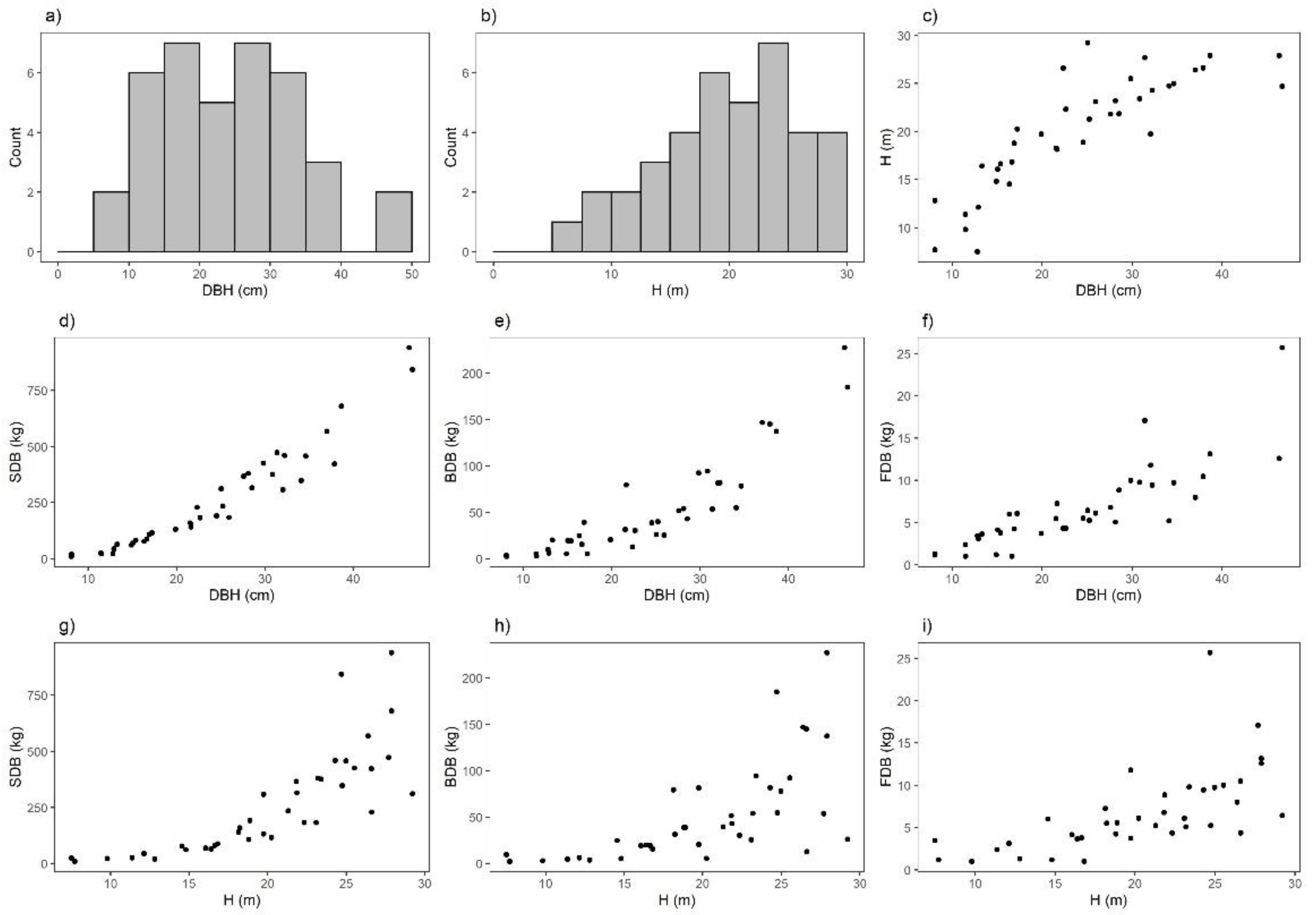
	Minimum	Maximum	Mean	Median	Standard Deviation
DBH	8.1	46.7	24.1	23.6	10.13
H	7.50	29.22	20.11	20.77	5.87
SDB	10	940	261	187	230
BDB	2	227	53	35	54
FDB	1	26	7	6	5

).

The felled trees were measured section-wise (1-m-long sections) and divided into the following biomass components: stem, branches, and foliage. All parts of each sample tree were weighed in the field using portable scales (precision 0.1 g). Samples of each of the components (stem discs in the middle of each section, and 50–150 g random samples of branches and foliage) from every tree were taken to determine the relationship between fresh and dry biomass. The samples were oven-dried at 105 °C until they reached a constant weight [40]. The dry biomass of various components (Table 2, Figure 1) was calculated for each sample tree based on corresponding fresh to dry mass ratios [41].

2.3. Individual Mixed-Effect Models

Two approaches were used when elaborating individual mixed-effects models. To ensure that the predicted variables are positive, the first approach involved modeling the dependence of dependent variables, as logarithms of dry biomass components (stem, branches, and foliage) and H-1.3, on DBH defined as the independent variable. In the second approach, the logarithms of dry biomass components and DBH were dependent variables, while H was defined as an independent variable. Thus, the general model for the dependent variable of tree j was:

$$\ln y_j= {\beta }_0+{\beta }_1{x}_j$$

(1)

For both approaches, linear mixed-effects modeling with sample plot as a single grouping factor (no other potential factors of grouping were present) was used. Each model for the tree j, j = 1, …, n_i of plot i, i = 1, …, M, was of the following form:

$$y_{ij}= {\mathit{x}}_{ij}^{\prime }\mathit{\beta }+{\mathit{z}}_{ij}^{\prime }{\mathit{b}}_i+{ϵ}_{ij}$$

(2)

where ${\mathit{x}}_{ij}^{\prime }\mathit{\beta }$ is the fixed part and ${\mathit{z}}_{ij}^{\prime }{\mathit{b}}_i+{ϵ}_{ij}$ describes the random part. Moreover, it is assumed that:

$${\mathit{b}}_i~N\left(\mathbf{0},\mathit{\psi }\right)$$

(3)

where ${\mathit{b}}_i$ are independent among plots and of the residual errors ${ϵ}_{ij}$. Matrix ψ is a positive definite variance–covariance matrix of random effects. The zero-mean residual errors ${ϵ}_{ij}$ were mutually independent, normally distributed, with variance calculated using the following formulas:

First approach [24]:

$$var\left(e_{ij}\right)={\sigma }^{2}DB{H}_{ij}{}^{\delta }$$

(4)

Second approach:

$$var\left(e_{ij}\right)={\sigma }^2{H}_{ij}{}^{\delta }$$

(5)

where ${\sigma }^2$ and $\delta$ are the estimated scale and shape parameters of the power function, respectively. The special case when δ = 0 leads to homoscedastic residuals.

2.4. Seemingly Unrelated Mixed-Effects Model System

Seemingly unrelated (multivariate) mixed-effects models with random group effects are useful in the case when several independent variables are measured for the same sample units. In this modeling context, random-effects prediction utilizes the cross-model correlations of the model system, thus taking into account the logical interactions between the biomass components. Moreover, their use in addition to the fixed-effects prediction enables to apply the relationship among the random effects and residuals across models for random-effects prediction. Assuming that we have L individual mixed-effects models and series of the observations of the mth of plot i to vector y_i^(m) and the corresponding model matrices of the fixed and random elements to X_i^(m) and Z_i^(m), the seemingly unrelated mixed-effects model system for each plot i, i = 1, …, m can be elaborated as [25,27]:

$$\begin{array}{c}{\mathit{y}}_i^{\left(1\right)}= {\mathit{X}}_i^{\left(1\right)}\mathit{\beta }+{\mathit{Z}}_i^{\left(1\right)}{\mathit{b}}_i{}^{\left(1\right)}+ {\mathit{ϵ}}_i^{\left(1\right)}\\ {\mathit{y}}_i^{\left(2\right)}= {\mathit{X}}_i^{\left(2\right)}\mathit{\beta }+{\mathit{Z}}_i^{\left(2\right)}{\mathit{b}}_i{}^{\left(2\right)}+ {\mathit{ϵ}}_i^{\left(2\right)}\\ ⋮\\ {\mathit{y}}_i^{\left(L\right)}= {\mathit{X}}_i^{\left(L\right)}\mathit{\beta }+{\mathit{Z}}_i^{\left(L\right)}{\mathit{b}}_i{}^{\left(L\right)}+ {\mathit{ϵ}}_i^{\left(L\right)}\end{array}$$

(6)

where $var\left({\mathit{b}}_i^{\left(l\right)}\right)={\mathit{\psi }}^{\left(l\right)}$ for l = 1,…,L. We assume that the cross-model correlations of the random effects and residuals are the same for all groups. The above multivariate model can be written as an univariate one:

$${\mathit{y}}_i= {\mathit{X}}_i\mathit{\beta }+{\mathit{Z}}_i{\mathit{b}}_i+ {\mathit{ϵ}}_i$$

(7)

where ${\mathit{y}}_i=\left({\mathit{y}}_i^{\left(1\right)\prime },{\mathit{y}}_i^{\left(2\right)\prime },\dots ,{\mathit{y}}_i^{\left(L\right)\prime }\right)\prime$, correspondingly for ${\mathit{b}}_i$ and ${\mathit{ϵ}}_i$ and ${\mathit{X}}_i$ and ${\mathit{Z}}_i$ are block-diagonal matrices, which have the response-specific model matrices on the diagonal [25,27].

2.5. Fixed- and Random-Effects Prediction

The main purpose of creating regression models is to use them for predicting dependent variable. The strength of mixed-effects models lies in the fact that, depending on the circumstances, it is possible to perform both fixed- and random-effects predictions, whereas the system of seemingly unrelated mixed-effects models allows to use also the cross-model correlations of random effects and residual errors to predict all dependent variables using measurements of some of them. This is possible by defining vectors that include only observed components and by defining matrices by removing rows and columns that correspond to the unobserved variables. During the analysis, the best linear predictor of the complete random effect vector is calculated, and the fixed part and variance–covariance matrices are replaced by their estimates, which leads to the EBLUP [25,27].

In this study, during plot-specific cross-model random-effects prediction, we used both seemingly unrelated mixed-effects model system approaches. To predict unobserved biomass components during calibration in the first and second approach, we used H and DBH as a measured dependent variable, respectively. In our case, dependent variables were predicted in a logarithmic scale. To transform them to the original scale we applied bias correction by adding half of the prediction variance into the predictions before applying the exponential transformation [42]. The fixed-effects approach was applied for 0 available trees in sample plot, whereas the cross-model random-effects prediction was created for two available extreme trees in sample plot [43]. We used DBH as their selection criterion. The remaining tree in sample plot was used to calculate the root mean square error (RMSE) based on the equation:

$$RMSE= \sqrt{\frac{{\displaystyle \sum }{\left(y_j-\widehat{y_j}\right)}^2}{n}}$$

(8)

where $y_j$ describes the observed value of the dependent variable, $\widehat{y_j}$ predicted value of the dependent variable, and $n$ explains the number of trees.

All analyses and graphs were performed using the nlme [44] and ggplot2 [45] packages of R 3.6.3 software [46] and RStudio 1.3.1073 [47].

3. Results

The use of the logarithm of the dependent variables and the linear individual mixed-effects models with a sample plot as a grouping factor sufficiently reflects the modeled dependencies for both the first and the second approach. In the case of the first approach, Akaike Information Criterion (AIC) for height equals −9.9, while for stem dry biomass, branches dry biomass, and foliage dry biomass, it equals 32.4, 69.7, and 57.9, respectively (Figure 2). In the case of the second approach, AIC for DBH equals 7.2, while for stem dry biomass, branches dry biomass, and foliage dry biomass, it equals 56.9, 104.5, and 78.2, respectively (Figure 3).

While analyzing the obtained residuals for both approaches of individual mixed-effect models, heteroscedasticity was identified. Application of the power function (Equations (4) and (5)) for residual variance modeling allowed achieving the stable distribution of residuals (Figure 4). Furthermore, a likelihood ratio test indicated that the variance function significantly improved the fit (p < 0.0001). The estimated fixed regression coefficients and variance function parameters of the model system are given in

Table 3. Estimated fixed parameters and standard errors (in brackets) for two approaches of seemingly unrelated mixed-effects model system.

First Approach
Dependent variable	SDB	BDB	FDB	H
${\beta }_0$	2.868 (0.319)	0.318 (0.434)	−0.371 (0.325)	2.593 (0.149)
${\beta }_1$	0.106 (0.014)	0.139 (0.019)	0.092 (0.013)	0.019 (0.005)
$\delta$	−0.25	−0.812	−0.629	−0.384
${\sigma }^2$	0.3672	4.3812	1.9972	0.332
Second Approach
Dependent variable	SDB	BDB	FDB	DBH
${\beta }_0$	1.401 (0.322)	−0.908 (0.448)	−0.623 (0.319)	1.526 (0.186)
${\beta }_1$	0.189 (0.016)	0.217 (0.023)	0.113 (0.015)	0.079 (0.009)
$\delta$	−0.179	−0.095	−0.332	−0.235
${\sigma }^2$	0.532	0.8652	1.3362	0.312

.

For the first approach of the model system, the random effects for H are strongly correlated with random effects estimated for biomass components. The strongest correlation is observed between H random effects and stem dry biomass (range from −0.981 to 0.978), while the weakest correlation is observed between H and foliage dry biomass (range from −0.579 to −0.549) (

Table 4. Random-effects variance–covariance matrix for two approaches of seemingly unrelated mixed-effects model system. Matrix diagonal—variance, matrix upper triangle—correlation between random effects.

First Approach
Dependent variable		SDB		BDB		FDB		H
		${\mathit{b}}_{\mathit{i}}^{\left(\mathbf{1}\right)}$	${\mathit{b}}_{\mathit{i}}^{\left(\mathbf{2}\right)}$	${\mathit{b}}_{\mathit{i}}^{\left(\mathbf{1}\right)}$	${\mathit{b}}_{\mathit{i}}^{\left(\mathbf{2}\right)}$	${\mathit{b}}_{\mathit{i}}^{\left(\mathbf{1}\right)}$	${\mathit{b}}_{\mathit{i}}^{\left(\mathbf{2}\right)}$	${\mathit{b}}_{\mathit{i}}^{\left(\mathbf{1}\right)}$	${\mathit{b}}_{\mathit{i}}^{\left(\mathbf{2}\right)}$
SDB	$b_i^{\left(1\right)}$	1.0952	−0.989	0.605	−0.849	0.419	−0.652	0.978	−0.981
	$b_i^{\left(2\right)}$	-	0.0482	−0.603	0.856	−0.357	0.620	−0.943	0.968
BDB	$b_i^{\left(1\right)}$	-	-	1.3942	−0.920	−0.027	−0.024	0.677	−0.748
	$b_i^{\left(2\right)}$	-	-	-	0.0662	−0.065	0.243	−0.873	0.931
FDB	$b_i^{\left(1\right)}$	-	-	-	-	1.0252	−0.926	0.417	−0.346
	$b_i^{\left(2\right)}$	-	-	-	-	-	0.0412	−0.597	0.549
H	$b_i^{\left(1\right)}$	-	-	-	-	-	-	0.5022	−0.984
	$b_i^{\left(2\right)}$	-	-	-	-	-	-	-	0.0172
Second Approach
Dependent variable		SDB		BDB		FDB		DBH
		${\mathit{b}}_{\mathit{i}}^{\left(\mathbf{1}\right)}$	${\mathit{b}}_{\mathit{i}}^{\left(\mathbf{2}\right)}$	${\mathit{b}}_{\mathit{i}}^{\left(\mathbf{1}\right)}$	${\mathit{b}}_{\mathit{i}}^{\left(\mathbf{2}\right)}$	${\mathit{b}}_{\mathit{i}}^{\left(\mathbf{1}\right)}$	${\mathit{b}}_{\mathit{i}}^{\left(\mathbf{2}\right)}$	${\mathit{b}}_{\mathit{i}}^{\left(\mathbf{1}\right)}$	${\mathit{b}}_{\mathit{i}}^{\left(\mathbf{2}\right)}$
SDB	$b_i^{\left(1\right)}$	0.8362	−0.975	0.530	−0.982	−0.493	−0.693	0.873	−0.952
	$b_i^{\left(2\right)}$	-	0.0412	−0.330	0.917	0.673	0.517	−0.744	0.862
BDB	$b_i^{\left(1\right)}$	-	-	0.4572	−0.679	0.475	−0.978	0.876	−0.763
	$b_i^{\left(2\right)}$	-	-	-	0.0332	0.323	0.815	−0.948	0.992
FDB	$b_i^{\left(1\right)}$	-	-	-	-	0.1292	−0.285	−0.007	0.205
	$b_i^{\left(2\right)}$	-	-	-	-	-	02	−0.957	0.880
DBH	$b_i^{\left(1\right)}$	-	-	-	-	-	-	0.5132	−0.980
	$b_i^{\left(2\right)}$	-	-	-	-	-	-	-	0.0242

). In the case of biomass components, the strongest correlation between random effects is between stem dry biomass and branches dry biomass (range from −0.849 to 0.856). For the second approach of the model system, the correlation between random effects of DBH and biomass components is within the range from −0.007 to −0.992 (Table 4). Similar to the first approach in the case of biomass components, the strongest correlation between random effects is between stem dry biomass and branches dry biomass (range from −0.330 to 0.982).

Comparing both approaches of the model system in terms of the correlation of the random effects of the non-biomass component with the biomass components, it is difficult to find an unambiguous trend. In the case of stem dry biomass, the strongest correlation is visible for H (first approach), while for branches dry biomass the strongest correlation between random effects occurs with DBH (second approach, Table 4).

The strongest correlation between residual errors for the first approach of the model system occurs for branches dry biomass and foliage dry biomass (0.557,

Table 5. Correlation between residual errors for both approaches of seemingly unrelated mixed-effects model system.

First Approach
Dependent variable	SDB	BDB	FDB
BDB	0.257	-	-
FDB	−0.100	0.557	-
H	0.474	−0.300	−0.287
Second Approach
Dependent variable	SDB	BDB	FDB
BDB	0.889	-	-
FDB	0.701	0.712	-
DBH	0.933	0.844	0.766

), while the weakest correlation is present between stem dry biomass and foliage dry biomass (–0.100). The strongest correlation between residual errors for the second approach is visible for stem dry biomass and diameter at breast height (0.933). Generally speaking, the stronger correlation between residual errors for all analyzed dependent variables occurs in the second approach of the model system (Table 5).

Fixed-effects prediction for the second approach allows reaching lower RMSE for biomass components than the fixed-effects prediction for the first approach (

Table 6. Root mean square error achieved during cross-model fixed and random-effects prediction for both approaches of seemingly unrelated mixed-effects model system.

First Approach
Dependent variable	SDB	BDB	FDB	H
Fixed-effects prediction	238.716	95.157	9.313	5.752
Random-effects prediction	77.603	36.018	6.887	3.297
Second Approach
Dependent variable	SDB	BDB	FDB	DBH
Fixed-effects prediction	206.933	67.366	3.726	8.868
Random-effects prediction	188.139	70.629	3.507	8.491

). Both H and DBH measurements for two extreme (the thickest and thinnest in sample plot) trees indicated that plot-specific cross-model random-effects prediction allowed to obtain a smaller RMSE than fixed-effects prediction. The only exception was branches dry biomass for the second approach. Random-effects prediction for the first approach allows reaching the smallest RMSE value (the exception is foliage dry biomass, Table 6).

4. Discussion and Conclusions

During this research, 38 felled trees from 13 sample plots located in West Poland were the basis for the elaboration of two approaches of a seemingly unrelated linear mixed-effects model system. In the first approach, the independent variable is the diameter at breast height, while in the second one, tree height. During analysis, both the fixed-effects and cross-model random-effects prediction in both approaches were taken into account. The sample plot was included as the grouping level. During random-effects prediction, tree height and diameter at breast height measurements for two available extreme trees in a plot in question were tested. Fitting of seemingly unrelated mixed-effects model system in both approaches enables the fixed-effects and cross-model random-effects prediction of aboveground dry biomass components (stem, branches, and foliage) of black locust.

When modeling individual biomass components, it is worth considering the logical assumption that the sum of the component of the tree estimated using equations should be equal to the estimated biomass of the whole tree. This assumption can be met by seemingly unrelated regression application [32,33,48,49]. The assumption about the additivity of the biomass model system and the use of nonlinear models was the basis of elaboration of a consistent set of additive biomass functions for eight tree species and nine components in Germany [34]. During that study, the authors defined two types of models: (i) a simple model with the diameter at breast height and height as independent variables, and (ii) a full model with more independent variables. Likewise, nonlinear seemingly unrelated regression was also used for nationwide biomass models covering the most common tree species of Canada’s forests [35]. Models fitted in this study allow us to estimate dry biomass of four components (stem wood, stem bark, branches, and foliage) using either diameter at breast height or, unlike our research, a combination of diameter at breast height and height. Likewise, in the case of seemingly unrelated empirical equations for estimating aboveground biomass of Betula pendula growing on former farmland in central Poland, diameter at breast height or diameter and tree height were defined as independent variables [36]. Seemingly unrelated empirical equations for the determination of the dry biomass of aboveground components for Scots pine in Poland also used diameter and height as independent variables [50], whereas simplified empirical formulas to determine the dry biomass of aboveground components of trees for Scots pine [51] and seemingly unrelated models for above- and belowground biomass for young silver birch [27] used diameter at breast height as the independent variable.

The cited studies are examples of using the seemingly unrelated regression with different approaches to the independent variables used. However, the knowledge of the authors indicates that no research has been undertaken yet that focuses on the development of independent model systems using diameter at breast height and height as independent variables. On the one hand, it is a new approach to biomass modeling, and on the other, due to the use of height as an independent variable, it increases the possibility of the practical application of the proposed solutions using remote data sources [52,53,54].

Since biomass data is often characterized by a grouped structure, mixed-effects models for biomass modeling could be used. The already-mentioned research is an example of this solution [34]. In this case, the authors took into account groups and trees as random effects, while Repola [55], during his research, elaborated three multivariate variance component models for the aboveground biomass components and one for the belowground biomass components. In this research, the multivariate model was based on diameter at breast height and height, and for the next multivariate models, additional commonly measured tree variables were used. It is worth to mention that unlike our research, Repola [55] included both the stand and tree-level during prediction, whereas Fehrmann [26], similar to our research, elaborated plot-specific linear mixed-effect biomass models. Notwithstanding, in his case, diameter at breast height and height were used at the same time as independent variables.

Due to the inclusion grouping data structure during modeling, the mixed-effects models allow the flexible prediction. In the absence of the measurement, data fixed effects can be used, whereas additional measurements allow increasing the accuracy through random-effects prediction [24,25]. However, in the case of biomass modeling, measurement of additional data is troublesome, because it is associated with the felling of trees. That is why multivariate mixed-effects model application allows taking full advantage of the mixed-effects models. In the case of our study, additional measurements of tree height (the first approach of the elaborated model system) and diameter at breast height (the second approach of the elaborated model system) allow us to reach more accurate random cross-model prediction for analyzed biomass components [28,29].

References

- Huntley, J.C. Robinia pseudoacacia L. black locust. In Silvic of North America 2. Hardwoods, Agriculture Handbook; Burns, R.M., Honkala, B.H., Eds.; United States Department of Agriculture (USDA), Forest Service: Washington, DC, USA, 1990; pp. 755–761. [Google Scholar]
- Nowiński, M. Dzieje Roślin i Upraw Ogrodniczych (History of Plants and Horticultural Crops); PWRiL: Warsaw, Poland, 1977. (In Polish) [Google Scholar]
- Vítková, M.; Müllerová, J.; Sádlo, J.; Pergl, J.; Pyšek, P. Black Locust (Robinia Pseudoacacia) Beloved and Despised: A Story of an Invasive Tree in Central Europe. For. Ecol. Manag. 2017, 384, 287–302. [Google Scholar] [CrossRef]
- Sitzia, T.; Cierjacks, A.; de Rigo, D.; Caudullo, G. Robinia pseudoacacia in Europe: Distribution, habitat, usage and threats. In European Atlas of Forest Tree Species; San-Miguel-Ayanz, J., de Rigo, D., Caudullo, G., Durrant, T.H., Mauri, A., Eds.; Publications Office of the European Union: Luxembourg, 2016; pp. 66–167. [Google Scholar]
- Kraszkiewicz, A. Evaluation of the Possibility of Energy Use Black Locust (Robinia Pseudoacacia L.) Dendromass Acquired in Forest Stands Growing on Clay Soils. J. Cent. Eur. Agric. 2013, 14, 388–399. [Google Scholar] [CrossRef]
- Bolat, I.; Kara, Ö.; Sensoy, H.; Yüksel, K. Influences of Black Locust (Robinia Pseudoacacia L.) Afforestation on Soil Microbial Biomass and Activity. Iforest Biogeosci. For. 2015, 9, 171–177. [Google Scholar] [CrossRef]
- Jagodziński, A.M.; Wierzcholska, S.; Dyderski, M.K.; Horodecki, P.; Rusińska, A.; Gdula, A.K.; Kasprowicz, M. Tree Species Effects on Bryophyte Guilds on a Reclaimed Post-Mining Site. Ecol. Eng. 2018, 110, 117–127. [Google Scholar] [CrossRef]
- Horodecki, P.; Nowiński, M.; Jagodziński, A.M. Advantages of Mixed Tree Stands in Restoration of Upper Soil Layers on Postmining Sites: A Five-Year Leaf Litter Decomposition Experiment. Land Degrad. Dev. 2019, 30, 3–13. [Google Scholar] [CrossRef] [Green Version]
- Qiu, L.; Zhang, X.; Cheng, J.; Yin, X. Effects of Black Locust (Robinia Pseudoacacia) on Soil Properties in the Loessial Gully Region of the Loess Plateau, China. Plant Soil 2010, 332, 207–217. [Google Scholar] [CrossRef]
- Rice, S.K.; Westerman, B.; Federici, R. Impacts of the Exotic, Nitrogen-Fixing Black Locust (Robinia Pseudoacacia) on Nitrogen-Cycling in a Pine-Oak Ecosystem. Plant Ecol. 2004, 174, 97–107. [Google Scholar] [CrossRef]
- Li, G.; Xu, G.; Guo, K.; Du, S. Mapping the Global Potential Geographical Distribution of Black Locust (Robinia Pseudoacacia L.) Using Herbarium Data and a Maximum Entropy Model. Forests 2014, 5, 2773–2792. [Google Scholar] [CrossRef] [Green Version]
- Rédei, K.; Csiha, I.; Keseru, Z.; Rásó, J.; Végh, Á.K.; Antal, B. Growth and Yield of Black Locust (Robinia Pseudoacacia L.) Stands in Nyírség Growing Region (North-East Hungary). South East Eur. For. 2014, 5, 13–22. [Google Scholar] [CrossRef] [Green Version]
- Nadal-Sala, D.; Hartig, F.; Gracia, C.A.; Sabaté, S. Global Warming Likely to Enhance Black Locust (Robinia Pseudoacacia L.) Growth in a Mediterranean Riparian Forest. For. Ecol. Manag. 2019, 449, 117448. [Google Scholar] [CrossRef]
- Puchałka, R.; Dyderski, M.K.; Vítková, M.; Sádlo, J.; Klisz, M.; Netsvetov, M.; Prokopuk, Y.; Matisons, R.; Mionskowski, M.; Wojda, T.; et al. Black Locust (Robinia Pseudoacacia L.) Range Contraction and Expansion in Europe under Changing Climate. Glob. Chang. Biol. 2021, 27, 1587–1600. [Google Scholar] [CrossRef]
- Tokarska-Guzik, B. The Establishment and Spread of Alien Plant Species (Kenophytes) in the Flora of Poland; Wydawnictwo Uniwersytetu Śląskiego: Katowice, Poland, 2005. [Google Scholar]
- Bronisz, K.; Zasada, M. Taper Models for Black Locust in West Poland. Silva Fenn. 2020, 54. [Google Scholar] [CrossRef]
- Wojda, T.; Klisz, M.; Jastrzębowski, S.; Mionskowski, M.; Szyp-Borowska, I.; Szczygieł, K. The Geographical Distribution Of The Black Locust (Robinia Pseudoacacia L.) In Poland And Its Role On Non-Forest Land. Pap. Glob. Chang. 2015, 22, 101–113. [Google Scholar] [CrossRef]
- Clark, D.A.; Brown, S.; Kicklighter, D.W.; Chambers, J.Q.; Thomlinson, J.R.; Ni, J. Measuring Net Primary Production in Forests: Concepts and Field Methods. Ecol. Appl. 2001, 11, 356–370. [Google Scholar] [CrossRef]
- IPCC Guidelines for National Greenhouse Gas Inventories: Reference Manual; UK Meteorological Office: Bracknell, UK, 1996.
- Cieszewski, C.J.; Zasada, M.; Lowe, R.C.; Liu, S. Estimating Biomass and Carbon Storage by Georgia Forest Types and Species Groups Using the FIA Data Diameters, Basal Areas, Site Indices, and Total Heights. Forests 2021, 12, 141. [Google Scholar] [CrossRef]
- Zianis, D.; Muukkonen, P.; Mäkipää, R.; Mencuccini, M. Biomass and Stem Volume Equations for Tree Species in Europe; Silva Fennica Monographs; Finnish Society of Forest Science, Finnish Forest Research Institute: Tampere, Finland, 2005. [Google Scholar]
- Zianis, D.; Mencuccini, M. Aboveground Biomass Relationships for Beech (Fagus moesiaca Cz.) Trees in Vermio Mountain, Northern Greece, and Generalised Equations for Fagus Sp. Ann. For. Sci. 2003, 60, 439–448. [Google Scholar] [CrossRef] [Green Version]
- Lehtonen, A.; Mäkipää, R.; Heikkinen, J.; Sievänen, R.; Liski, J. Biomass Expansion Factors (BEFs) for Scots Pine, Norway Spruce and Birch According to Stand Age for Boreal Forests. For. Ecol. Manag. 2004, 188, 211–224. [Google Scholar] [CrossRef]
- Pinheiro, J.; Bates, D. Mixed-Effects Models in S and S-PLUS; Springer: New York, NY, USA, 2013. [Google Scholar]
- Mehtätalo, L.; Lappi, J. Forest Biometrics with Examples in R; Chapman & Hall/CRC: New York, NY, USA, 2020. [Google Scholar]
- Fehrmann, L.; Lehtonen, A.; Kleinn, C.; Tomppo, E. Comparison of Linear and Mixed-Effect Regression Models and a k-Nearest Neighbour Approach for Estimation of Single-Tree Biomass. Can. J. For. Res. 2008, 38, 1–9. [Google Scholar] [CrossRef]
- Bronisz, K.; Mehtätalo, L. Seemingly Unrelated Mixed-Effects Biomass Models for Young Silver Birch Stands on Post-Agricultural Lands. Forests 2020, 11, 381. [Google Scholar] [CrossRef] [Green Version]
- Lappi, J. Calibration of Height and Volume Equations with Random Parameters. For. Sci. 1991, 37, 781–801. [Google Scholar]
- Bronisz, K.; Mehtätalo, L. Mixed-Effects Generalized Height–Diameter Model for Young Silver Birch Stands on Post-Agricultural Lands. For. Ecol. Manag. 2020, 460, 117901. [Google Scholar] [CrossRef]
- Ou, G.; Wang, J.; Xu, H.; Chen, K.; Zheng, H.; Zhang, B.; Sun, X.; Xu, T.; Xiao, Y. Incorporating Topographic Factors in Nonlinear Mixed-Effects Models for Aboveground Biomass of Natural Simao Pine in Yunnan, China. J. For. Res. 2016, 27, 119–131. [Google Scholar] [CrossRef]
- Pearce, H.G.; Anderson, W.R.; Fogarty, L.G.; Todoroki, C.L.; Anderson, S.A.J. Linear Mixed-Effects Models for Estimating Biomass and Fuel Loads in Shrublands. Can. J. For. Res. 2010, 40, 2015–2026. [Google Scholar] [CrossRef]
- Kozak, A. Methods for Ensuring Additivity of Biomass Components by Regression Analysis. For. Chron. 1970, 46, 402–405. [Google Scholar] [CrossRef]
- Parresol, B.R. Assessing Tree and Stand Biomass: A Review with Examples and Critical Comparisons. For. Sci. 1999, 45, 573–593. [Google Scholar]
- Vonderach, C.; Kändler, G.; Dormann, C.F. Consistent Set of Additive Biomass Functions for Eight Tree Species in Germany Fit by Nonlinear Seemingly Unrelated Regression. Ann. For. Sci. 2018, 75, 49. [Google Scholar] [CrossRef] [Green Version]
- Ung, C.-H.; Bernier, P.; Guo, X.-J. Canadian National Biomass Equations: New Parameter Estimates That Include British Columbia Data. Can. J. For. Res. 2008, 38, 1123–1132. [Google Scholar] [CrossRef]
- Bronisz, K.; Strub, M.; Cieszewski, C.; Bijak, S.; Bronisz, A.; Tomusiak, R.; Wojtan, R.; Zasada, M. Empirical Equations for Estimating Aboveground Biomass of Betula Pendula Growing on Former Farmland in Central Poland. Silva Fenn. 2016, 50. [Google Scholar] [CrossRef] [Green Version]
- Martyn, D. Klimaty Kuli Ziemskiej (Climates of the Earth); PWN: Warsaw, Poland, 2000. (In Polish) [Google Scholar]
- European Climate Assessment & Dataset. Available online: https://www.ecad.eu (accessed on 5 February 2021).
- Bronisz, K.; Bijak, S.; Wojtan, R.; Tomusiak, R.; Bronisz, A.; Baran, P.; Zasada, M. Biomass_Black_Locuts.xlsx. 2021. Available online: https://figshare.com/articles/dataset/Biomass_Black_Locuts_xlsx/13721107/1 (accessed on 23 March 2021). [CrossRef]
- Samuelsson, R.; Burvall, J.; Jirjis, R. Comparison of Different Methods for the Determination of Moisture Content in Biomass. Biomass Bioenergy 2006, 30, 929–934. [Google Scholar] [CrossRef]
- Snowdon, P.; Raison, J.; Keith, H.; Ritson, P.; Grierson, P.; Adams, M.A.; Montagu, K.; Hui-quan, B.; Burrows, W.; Eamus, D. Protocol for Sampling Tree and Stand Biomass; Australian Greenhouse Office: Canberra, Australia, 2002. [Google Scholar]
- Baskerville, G.L. Use of Logarithmic Regression in the Estimation Of plant Biomass. Can. J. For. Res. 1972, 2, 49–53. [Google Scholar] [CrossRef]
- Pukelsheim, F. Optimal Design of Experiments; Classics in Applied Mathematics; Society for Industrial and Applied Mathematics, University City: Philadelphia, PA, USA, 2006. [Google Scholar]
- Pinheiro, J.; Bates, D.; Saikat, D.; Deepayan, S. Nlme: Linear and Nonlinear Mixed Effects Models; 2020; Available online: https://cran.r-project.org/web/packages/nlme/index.html (accessed on 23 March 2021).
- Wickham, H. Ggplot2: Elegant Graphics for Data Analysis; Springer: New York, NY, USA, 2016. [Google Scholar]
- R Core Team. R: A Language and Environment for Statistical Computing; R Foundation for Statistical Computing: Vienna, Austria, 2020. [Google Scholar]
- RStudio Team. RStudio: Integrated Development for R; RStudio Inc.: Boston, MA, USA, 2015. [Google Scholar]
- Cunia, T.; Briggs, R.D. Forcing Additivity of Biomass Tables—Some Empirical Results. Can. J. For. Res. 1984, 14, 376–384. [Google Scholar] [CrossRef]
- Chiyenda, S.S.; Kozak, A. Additivity of Component Biomass Regression Equations When the Underlying Model Is Linear. Can. J. For. Res. 1984, 14, 441–446. [Google Scholar] [CrossRef]
- Zasada, M.; Bronisz, K.; Bijak, S.; Wojtan, R.; Tomusiak, R.; Dudek, A.; Michalak, K.; Wróblewski, L. Wzory Empiryczne Do Określania Suchej Biomasy Nadziemnej Części Drzew i Ich Komponentów (Empirical Formulae for Determination of the Dry Biomass of Aboveground Parts of the Tree). Sylwan 2008, 152, 27–39. (In Polish) [Google Scholar] [CrossRef]
- Bronisz, K.; Zasada, M. Uproszczone Wzory Empiryczne Do Określania Suchej Biomasy Nadziemnej Części Drzew i Ich Komponentów Dla Sosny Zwyczajnej (Simplified Empirical Formulas to Determine the Dry Biomass of Aboveground Components of Trees for Scots Pine). Sylwan 2016, 160, 277–283. (In Polish) [Google Scholar] [CrossRef]
- Vauhkonen, J.; MehtÄtalo, L.; Packalén, P. Combining Tree Height Samples Produced by Airborne Laser Scanning and Stand Management Records to Estimate Plot Volume in Eucalyptus Plantations. Can. J. For. Res. 2011, 41, 1649–1658. [Google Scholar] [CrossRef]
- Maltamo, M.; Mehtätalo, L.; Vauhkonen, J.; Packalén, P. Predicting and Calibrating Tree Attributes by Means of Airborne Laser Scanning and Field Measurements. Can. J. For. Res. 2012, 42, 1896–1907. [Google Scholar] [CrossRef]
- Stereńczak, K.; Zasada, M. Accuracy of Tree Height Estimation Based on LIDAR Data Analysis. Folia For. Pol. 2011, 53, 123–129. [Google Scholar]
- Repola, J. Biomass Equations for Birch in Finland. Silva Fenn. 2008, 42, 605–624. [Google Scholar] [CrossRef] [Green Version]