Article

Future Impacts of Land Use Change on Ecosystem Services under Different Scenarios in the Ecological Conservation Area, Beijing, China

Beijing Key Laboratory of Forest Resources and Ecosystem Processes, Beijing Forestry University, Beijing 100083, China
*
Author to whom correspondence should be addressed.
Forests 2020, 11(5), 584; https://doi.org/10.3390/f11050584
Submission received: 13 April 2020 / Revised: 18 May 2020 / Accepted: 21 May 2020 / Published: 22 May 2020
(This article belongs to the Section Forest Ecology and Management)

Abstract

:
Ecosystem services (ES), defined as benefits provided by the ecosystem to society, are essential to human well-being. However, it remains unclear how they will be affected by land-use changes due to lack of knowledge and data gaps. Therefore, understanding the response mechanism of ecosystem services to land-use change is critical for developing systematic and sound land planning. In this study, we aimed to explore the impacts of land-use change on the three ecosystem services, carbon storage (CS), flood regulation (FR), and soil conservation (SC), in the ecological conservation area of Beijing, China. We first projected land-use changes from 2015 to 2030, under three scenarios, i.e., Business as Usual (BAU), Ecological Land Protection (ELP), and Rapid Economic Development (RED), by interactively integrating the Markov model (Quantitative simulation) with the GeoSOS-FLUS model (Spatial arrangement), and then quantified the three ecosystem services by using a spatially explicit InVEST model. The results showed that built-up land would have the most remarkable growth during 2015–2030 under the RED scenario (2.52% increase) at the expense of cultivated and water body, while forest land is predicted to increase by 152.38 km2 (1.36% increase) under the ELP scenario. The ELP scenario would have the highest amount of carbon storage, flood regulation, and soil conservation, due to the strict protection policy on ecological land. The RED scenario, in which a certain amount of cultivated land, water body, and forest land is converted to built-up land, promotes soil conservation but triggers greater loss of carbon storage and flood regulation capacity. The conversion between land-use types will affect trade-offs and synergies among ecosystem services, in which carbon storage would show significant positive correlation with soil conservation through the period of 2015 to 2030, under all scenarios. Together, our results provide a quantitative scientific report that policymakers and land managers can use to identify and prioritize the best practices to sustain ecosystem services, by balancing the trade-offs among services.

1. Introduction

Ecosystem services (ES) can be defined as the various benefits—including products and services—that peoples obtain from ecosystems that contribute to human well-being or maintain the global life-supporting systems [1,2,3]. In the last several decades, high demands for natural resources such as food, fuel, and shelter arising from population growth, rapid urbanization, and economic development have redoubled human efforts to enhance certain ecosystem services [4], often at the expense of others [5]. As a result, human activities have changed global ecosystems with unprecedented intensities and rates. According to Millennium Ecosystem Assessment (MEA), over 60% of global ecosystem services have degraded and therefore affected the provision of current and future ecosystem services [2]. Among all human activities, land-use change is one of the major determinants of the supply of ES [2,6,7,8,9], as certain ES are closely correlated to specific types of land use [1,10]; for example, timber and climate regulation are mostly provided by forests [11]. Therefore, the relationship between land-use change and ES is receiving extensive attention by scientists and policymakers worldwide.
In this context, several studies have made progress in elucidating ES supply changes and the effects of land-use changes [12,13,14,15]. The influences of land-use changes on ES vary widely across different socioeconomic backgrounds and spatial or temporal scales [5,16]. Recent research has demonstrated that the diversity of social demands and the spatial heterogeneity of environment result in more complex and constantly changing interactions among multiple ecosystems’ services [17,18]. For instance, the increase of cultivated land for food leads to reductions in carbon storage and increased risk of soil erosion, while urbanization—which can result in reforestation and improved human living environments—can disrupt surface water balance and influence regional climates [19,20]. These finding exemplify how promotion of one particular ES by land-use change often leads to gains or losses of other ES, suggesting the existence of synergies or trade-offs in the provisioning of ES [21,22]. Although they are not always obvious, synergies or trade-offs among multiple ES are taking place all the time, which are often poorly understood and thus may cause unintended environmental consequences. Therefore, reassessing our assumptions surrounding land-use change with greater focus on the trade-offs among multiple ES driven by the interactions among land-use types will provide a theoretical basis for land-use managers and policymakers.
The relationship between ES and land-use changes highlights the importance of ES in guiding land-use planning and ecosystem management strategies to promote sustainability [23,24,25]. Specifically, ES assessments can be integrated into land-use planning in two modes; one is used as a criterion in land-use scheme development. For instance, [26] utilized the land-use optimization model FUTURES that is based on the bottom-up Cellular Automata (CA) simulation and the state transformation of micro-level cells to examine the impact of three urban growth scenarios on ES. The other is as an assessment, comparison, and selection among multiple land-use schemes under different scenarios. For instance, [23] predicted the urban expansion and ES dynamics in Beijing from 2013 to 2040 under different development scenarios. They found that decreases of some critical ecosystem services would be significantly lower under a scenario to conserve ecosystem services than those under the business-as-usual scenario. Moreover, [27] evaluated the impacts of different urban growth scenarios on four ES, to determine the degree to which configuration of urbanization and the development of natural land-use/land-cover impacts these services and trade-offs over 25 years in Western North Carolina. However, due to the uncertainty of alternative future land-use dynamics relative to socioeconomic and natural environmental driving forces [9], assessing how the ecosystem services and their trade-offs and synergies will temporally respond to future land-use changes remains challenging. Although spatiotemporal land-use scenario simulations are an effective and reproducible tool in projecting future land-use trajectories and support future land-use policy decisions [28,29], most of these models can only simulate the dynamics of one individual land-use class, as different land-use/land-cover changing processes occur simultaneously and interact with each other in most cases. Thus, we propose an approach that interactively integrates the Markov model (Quantitative simulation) with the GeoSOS-FLUS model (Spatial arrangement) for a multiple land-use dynamic simulation, which couples both human-related and natural environmental effects, using an elaborate design of the interactions and competition among different land-use types under alternative scenarios.
Over the past few decades, rapid economic development and population growth, accompanied by drastic land-use changes, have triggered ecological crises like water shortages, soil erosion, and losses of high-quality cultivated land, which are among the most serious problems that Beijing faces—especially in the western and northern mountainous areas [30]. Although there has been the protection of laws for the nature reserves and other legally binding of ecological zones, they are not respected and are seriously threatened in the current land-use policies. To address these problems, local governments initiated a series of ecological protection plans, including the “Red Lines for Ecological Protection in Beijing”, as well as the “13th Five-Year Plan of Environmental protection and Ecological construction in Beijing”. Here, we use the ecological conservation area of Beijing, an area with intense human activities and ecologically vulnerable areas, as the study area. In this area, the complex interaction between human activities and the natural environment poses a major challenge to the sustainable provision of ES. Therefore, we first present the future land-use simulation (GeoSOS-FLUS) model and Markov model to simulate future land use under three alternative scenarios, i.e., Business as Usual (BAU), Rapid Economic Development (RED), and Ecological Land Protection (ELP) in the ecological conservation area. Then, we selected the InVEST (Integrated Valuation of Ecosystem Services and Trade-Offs) model that was developed by the Natural Capital Project team of the United States and has been widely used in evaluating the quantity of ecosystem services and to support ecosystem management and decision-making. Specifically, we focus on three main objectives: (1) modeling the current and future dynamics of the ES—carbon storage (CS), flood regulation (FR), and soil conservation (SC); (2) quantifying the effects of land-use change on these services and the trade-offs among them; (3) providing appropriate indicators to support the identification of rational land-use strategies, to improve ES management for our study area.

2. Materials and Methods
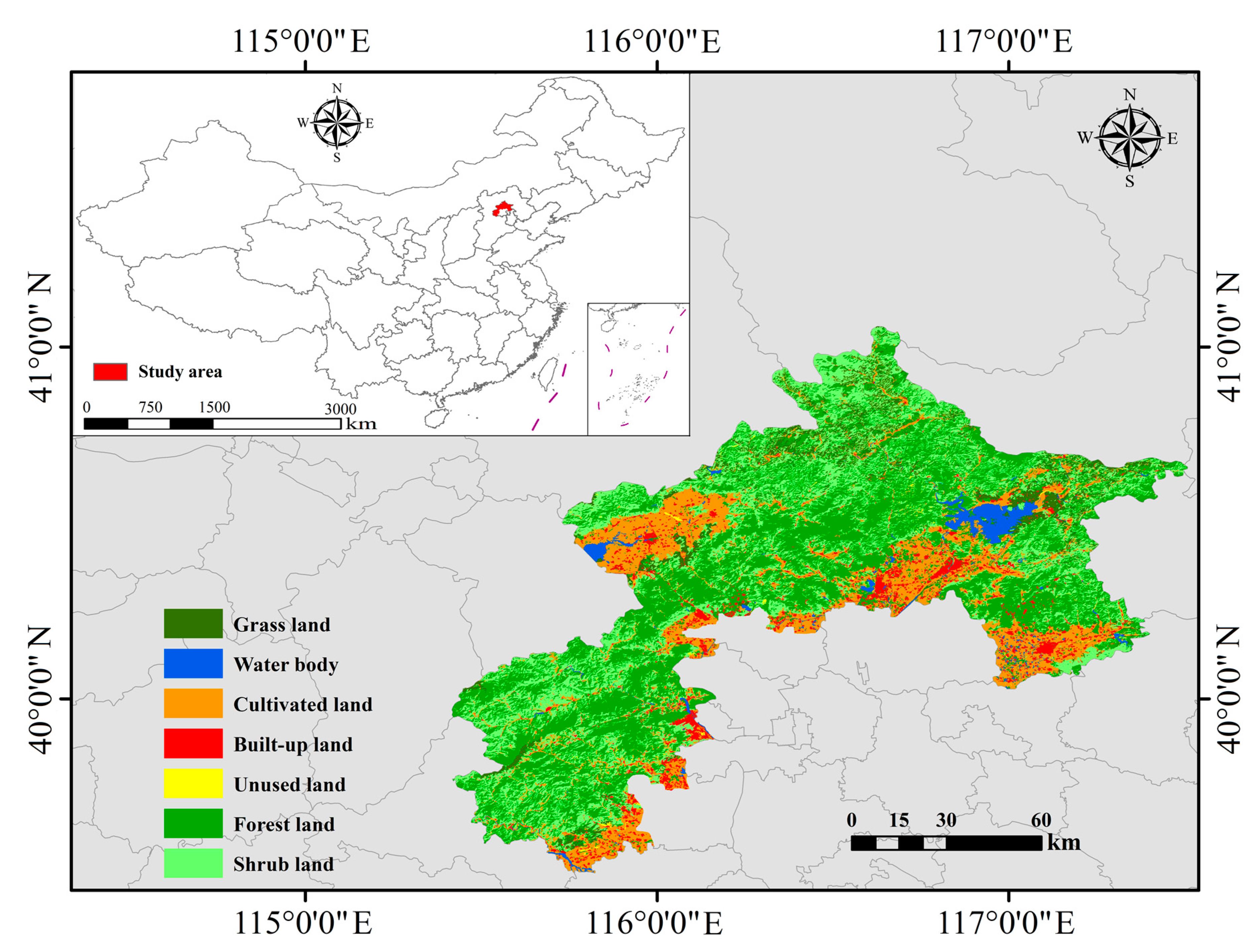
2.1. Study Area

The ecological conservation area (41°04′–39°31′N, 115°24′–117°29′) is located in Northwestern Beijing, China (Figure 1). The study area, accounting for approximately 53.3% of the entire area of the city, covers a total area of 11,140.15 km2. This region is very mountainous region—with altitudes varying from 11 to 2304 m—with a typical temperate monsoon climate: average annual precipitation of 576.71 mm from 2000 to 2015, in which the primary rainfall occurs in the rainy season, from June to August, and monthly average temperature that ranges from 2.5 to 13.4 °C (Reanalysis of climate data from the Resources and Environmental Sciences, Chinese Academy of Sciences (http://www.resdc.cn/)). The ecological conservation area is characterized by rich biodiversity and diverse ecosystems that include the region’s most important mountain areas, water sources, ecological forests, basic cultivated land, and other core ecological elements [31]. In recent decades, this region has experienced rapid urbanization and economic growth, accompanied by increasing environmental concerns [9]. Therefore, it has been specially protected and identified as a key area in ensuring Beijing’s sustainable development by the People’s Government of Beijing Municipality.

2.2. Data Requirement and Preparation

Gridded land-use maps of the ecological conservation area in 2000 and 2015 (30 m spatial resolution) were obtained from the Resources and Environmental Sciences, Chinese Academy of Sciences (http://www.resdc.cn/). The dataset is based on the supervised classification of Landsat TM images, using ENVI Imagine software, and uses seven land classes: forest land, cultivated land, water body, grassland, shrub land, built-up land, and unused land (see descriptions in Supplementary Table S1). In addition, another five data types were used in the InVEST model: (1) 30 m resolution SRTM V4.1, Digital Elevation Model (DEM) obtained from National Catalogue Service for Geographic Information (http://www.webmap.cn/); (2) 1 km resolution meteorological data, including annual precipitation, monthly precipitation, temperature, and sunshine hours provided by the National Earth System Science Data Center (http://www.geodata.cn/); (3) 1 km resolution data related to soil attributes, root restricting layer depth, and plant AWC obtained from the Harmonized World Soil Database (http://webarchive.iiasa.ac.at/Research/LUC/External-World-soil-database/); (4) evapotranspiration coefficient (Kc) values for crops from the Food and Agriculture Organization of the United Nations (FAO) (http://www.fao.org/3/X0490E/x0490e0b.htm); and (5) carbon stored in the four basic carbon pools for each land-use type, obtained from previous studies of Beijing City [32]. We used ArcGIS 10.3 for GIS analyses, in which all spatial raster data were converted to the same projection coordinate system (Beijing_1954_3_Degree_GK_CM_ 114E) and a spatial resolution of 30 m. The input data are presented in Table 1.

2.3. Future Scenarios Design

In this study, land use in 2030, under three scenarios, was modeled, using the Markov and future land-use simulation (GeoSOS-FLUS) models, which incorporated socioeconomic and ecological characteristics in different scenarios [33,34]. We used a 2015 land-use map as a baseline year for comparison under three alternative future scenarios. The climate, including annual temperature and precipitation, is assumed to maintain the current state.

2.3.1. Business as Usual (BAU)

We developed the BAU scenario based on the trajectory of land-use transitions over the past 15 years in the ecological conservation area. We assumed that the social, economic, and land-use evolution trends remain unchanged from 2015 to 2030 under the BAU scenario. Thus, the rate of land-use change is considered to agree with the annual change from 2000 to 2015 (Supplementary Materials Figure S1 and Table S3). The Markov models were used to simulate the land-use demand.

2.3.2. Ecological Land Protection (ELP)

The ELP scenario can be viewed as a harmonious development scenario for 2030 that aims to develop a more human-oriented and sustainable development mode by the local government. This scenario is characterized by condensed and slower urbanization in which the environment will be considered. This scenario gives priority to the existing ecological protection measures, including protecting Miyun reservoir, natural reserves, primary farmlands, and park green spaces, which are restricted from being converted to other lands. Moreover, under the ELP scenario, the area of built-up land would show a slight increase and forest land would increase more than other scenarios, up to 2030. The area of cultivated land (paddy fields and dry land) would be held above 7% of the study area based on the Beijing’s General Urban Planning (2016–2035). This scenario will reduce the speed of urban growth and the negative effects of urban expansion on ecosystem services.

2.3.3. Rapid Economic Development (RED)

The RED scenario is based on the BAU scenario but includes rapid urbanization in the study area. We assumed that rapid increases of population and technologies, as well as economic development, would occur in the process of urban development from 2015 to 2030, under this scenario. At the same time, the demands for built-up land, including urban and rural residential land, construction land, and transport facility areas, would expand rapidly. To be specific, built-up land would be concentrated in the lower part of the study area and increase more than the other two scenarios. To meet the growing population’s demand for food, cultivated land will experience less of a decline than the BAU scenario. In addition, basic farmland protection areas should be added in the restricted area.

2.4. Future Land-Use Modeling

In this study, we projected different land use for alternative scenarios, using the (1) Markov model to estimate quantitative demands of different land-uses in 2030 and (2) GeoSOS-FLUS model to estimate spatial patterns in 2030. The mutual feedback between demand model and GeoSOS-FLUS model generate the simulated land-use maps at the end of the simulation period [35].

2.4.1. Land-Use Demand Projection

The Markov model, as a non-spatial demand of future land use, was used to generate the conversion probability of land-use types over a time series [36,37]. The land-use maps of different time intervals were exported from simulations and compared with each other, in the form of matrices, based on maximum values of probability [37,38]. The maximum probability for each grid cell to either remain unchanged or convert to another class was calculated. Finally, the Markov model was applied to our study area from 2015–2030, using the probability transition matrix and transition maps of each class to another class from 2000 to 2015, under the following equation:
Sij(t+1) = PijSi(t)
where Sij(t+1) is the state of land-use type i converting to j at the future time of t+1; Si(t) is the state of land-use type i at time t; and Pij is the transition probability of land-use type i to j.

2.4.2. Land-Use Spatial Pattern Simulation

The cellular automata (CA) model was designed to project spatial patterns of future land use, under the given land-use demands determined by the non-spatial module. Within the CA allocation procedure, the following two steps were implemented: (1) An artificial neural network (ANN) algorithm was used to train and predict the probability of occurrence of each land-use type on a specific grid [39], and (2) a self-adaptive inertia and competition mechanism was designed to address the competition and interactions among different land-use types [34,40]. Driving factors and data of land-use change were selected from the available literature and tested as predicting variables (Supplementary Table S2) [34,41].
The ANN was composed of prediction and training stages, whose calculation formula is as follows:
sp ( p , k , t ) = j w j , k × s i g m o i d ( n e t j ( p , t ) ) = j w j , k × 1 1 + e n e t j ( p , t )
where s p ( p , k , t ) is the probability of suitability of land-use type k at time t and grid cell p; w j , k is the weight between the output layer and the hidden layer; Sigmoid () is the excitation function from the hidden layer to the output layer; and n e t j ( p , t ) is the signal received by the jth hidden grid cell p at time t. The sum of suitability probabilities of each land-use type output by the ANN is always 1:
k s q ( p , k , t ) = 1
In this mechanism, a self-adaptive inertia coefficient for different types of land use is defined to adjust the difference between current allocated land amount and land demand in the iterative process. The coefficient of kth land use at time t is I n t e r t i a k t , given by:
I n t e r t i a k t { I n t e r t i a k t 1                             | D k t 1 | | D k t 2 |     I n t e r t i a k t 1 × D k t 2 D k t 1                 0 > D k t 2 > D k t 1       I n t e r t i a k t 1 × D k t 1 D k t 2                 D k t 1 > D k t 2 > 0
where D k t 1 and D k t 2 are the differences between the demand and allocated amount of land-use type k at time t-1 and t-2, respectively. By calculating the above two formulas, the probability of land-use types at each grid cell is estimated, and the dominant land-use type is allocated to this grid cell during a CA model iteration. The probability T P p , k t of grid p converting to land-use type k at time t is thus calculated as follows:
T P p , k t = s p ( p , k , t ) × Ω p , t t × I n t e r t i a k t × ( 1 s c c k )
where s c c k is the cost of converting from original land-use type c to the target land-use type k; 1 s c c k is the difficulty level of the conversion; and Ω p , t t is the neighborhood effect of land-use type k on grid cell p at time t.

2.4.3. Model Implementation and Precision Validation

We tested and compared the performance of the FLUS model by simulating land-cover changes from 2000 to 2015. The land-use spatial distribution in 2000 was regarded as the base map of simulation; other inputs included the simulation parameters, the restricted areas, and driving data. After running the GeoSOS-FLUS model for 15 years, a simulated land-use map for 2015 was obtained. We selected the FoM (Figure of Merit) indicator to measure the performance of the simulation results for land-cover change from 2000 to 2015, as it avoids the disadvantage of overestimating the accuracy in traditional validation methods (e.g., the overall accuracy and the Cohen’s Kappa coefficient) [42,43]. The FoM can be mathematically expressed as the ratio of the correct predicted change to the sum of the observed change and predicted change. The value of FoM, ranging from 0% to 100%, reflects the simulation accuracy by focusing only on the part of the land that has changed, with 100% representing the perfect fitting between the observed and simulated changes. The resulting FoM value (0.269) was similar to or greater than those of other case studies on land-cover-change modeling, as previous comparative analyses have demonstrated that the common values of FoM ranged from 10% to 30% for existing land-use-change models [44,45,46]. This result indicated that the performance of our model was reliable. Thus, the parameters and driving data within this model are acceptable and can be applied to predict future land-use patterns (Supplementary Table S2). Hence, we used the abovementioned validated parameters and the classified land-use map in 2015 to simulate land use in 2030 under three scenarios.

2.5. Quantifying Ecosystem Services

The current and future ecosystem services (ES) were modeled by using the spatially explicit InVEST (version 3.8.0.) model, based on land-use maps of current and future scenarios in the ecological conservation area [47,48,49]. We focused on the following three ecosystem services: carbon storage (CS), flood regulation (FR), and soil conservation (SC). These priority ES represent the main and important categories in relation to climatic, terrain, and soil conditions. The quantification and spatial mapping of ecosystem services were done within the InVEST model, utilizing a series of parameters and data.

2.5.1. Carbon Storage (CS)

The amount of carbon stored and sequestered was calculated based on the land-use and climate information of carbon stocks within each respective time period and simulated scenario, using the tool “Carbon Storage and Sequestration: Climate Regulation” of the InVEST model. This model aggregates the amount of carbon stored in four major carbon pools, aboveground biomass, belowground biomass, soil, and dead organic matter, with land-use maps and particular classification (see Supplementary Table S4) [49]. We calculated the total carbon stored, CSjxy, for each given grid cell (x,y) with land-use type, j, as follows:
CSjxy = Ax (Cajxy + Cbjxy + Csjxy + Cdjxy)
where Cajxy, Cbjxy, Csjxy, and Cdjxy are carbon densities in aboveground biomass (Mg C ha−1), belowground biomass (Mg C ha−1), soil (Mg C ha−1), and dead matter (Mg C ha−1) for the grid cell (x,y) with land-use type j, respectively.

2.5.2. Flood Regulation (FR)

Flood regulation service referred to the capacity of a landscape to retain storm-water runoff. The “Annual Water Yield” module of InVEST model was used to quantify the water yield from each grid cell, with mean annual precipitation, depth of soil (mm), plant available water content, annual potential evapotranspiration, and land use (see Supplementary Table S5) [49]. The calculations of annual water yield, Yx, for each pixel on the landscape x were as follows:
Yx = (1−AETx/Px) · Px
AETx/Px = (1 + PETx/Px) - [1 + (PETx/Px)ω]1/ω
PETx = Kx · ET0/Px
ωx = Z · AWCx/Px + 1.25
AWCx = Min (Rest. layer. Soil Depth, Root. Depth) · PAWC
where AETxj is the annual actual evapotranspiration for pixel x, and Px is the annual precipitation on pixel x. AETx/Px is based on an expression of the Budyko curve developed by [50,51]; PETx is the potential evapotranspiration, and ωx is a an empirical parameter that characterizes the natural climatic-soil properties; ET0 is the reference evapotranspiration, and Kx is the coefficient of vegetation evapotranspiration [49]; AWCx is the volumetric plant available water content; and Z is an empirical constant, sometimes referred to as “seasonality factor”, which ranges from 1 to 30, and needs to be calibrated with monitoring data from the local precipitation pattern and hydrogeological characteristics [49]. PAWC is the plant available water capacity (0–1).

2.5.3. Soil Conservation (SC)

The “sediment delivery ratio” module of InVEST model was applied to estimate the annual processes of catchment soil loss, sediment transport into river channels, and sediment interception by vegetation and topography, which works on the spatial resolution of the input DEM raster [49]. Following previous studies [52,53], we used the Revised Universal Soil Loss Equation (RUSLE) to calculate annual soil loss for each pixel, based on the rainfall erosivity and soil erodibility, along with biophysical attributes related to sediment retention based on land cover. Reductions of soil loss indicate that there was an improvement in soil conservation. The calculations of SC for pixel i are as follows:
SCi = RKLSiuslei
uslei = Ri · Ki · Li · LSi · Ci · Pi
RKLSi = Ri · Ki · Li · Si
where SCi is the amount of annual soil conservation (ton·(hm2·a)−1); RKLSi is the amount of potential soil loss in pixel i (ton·(hm2·a)−1); uslei is the amount of actual soil loss in pixel i (ton·(hm2·a)−1); Ri is the rainfall erosivity factor (MJ·mm·(ha·hr)−1); Ki is the soil erodibility factor (ton·ha·hr·(MJ·ha·mm)−1); LSi is the length-gradient factor (unitless); Si is the slope factor (unitless); and Ci and Pi represent the crop-management and support practice factors (both unitless), respectively (see Supplementary Table S6).

2.6. Assessment of the Trade-Offs/Synergies among ES

Trade-offs/synergies among ES were expressed with correlation coefficients. First, we applied the “Create Random Points” tool in ArcGIS 10.3 to create random sample points, and then we extracted the ecosystem service value of each sample point, using the “Extract Multiple Values to points” method. The total number of samples selected for this study is 5000. Finally, the correlation coefficients were calculated by using SPSS 24 statistical software based on the service value of these points (Pearson, two-tailed).

3. Results

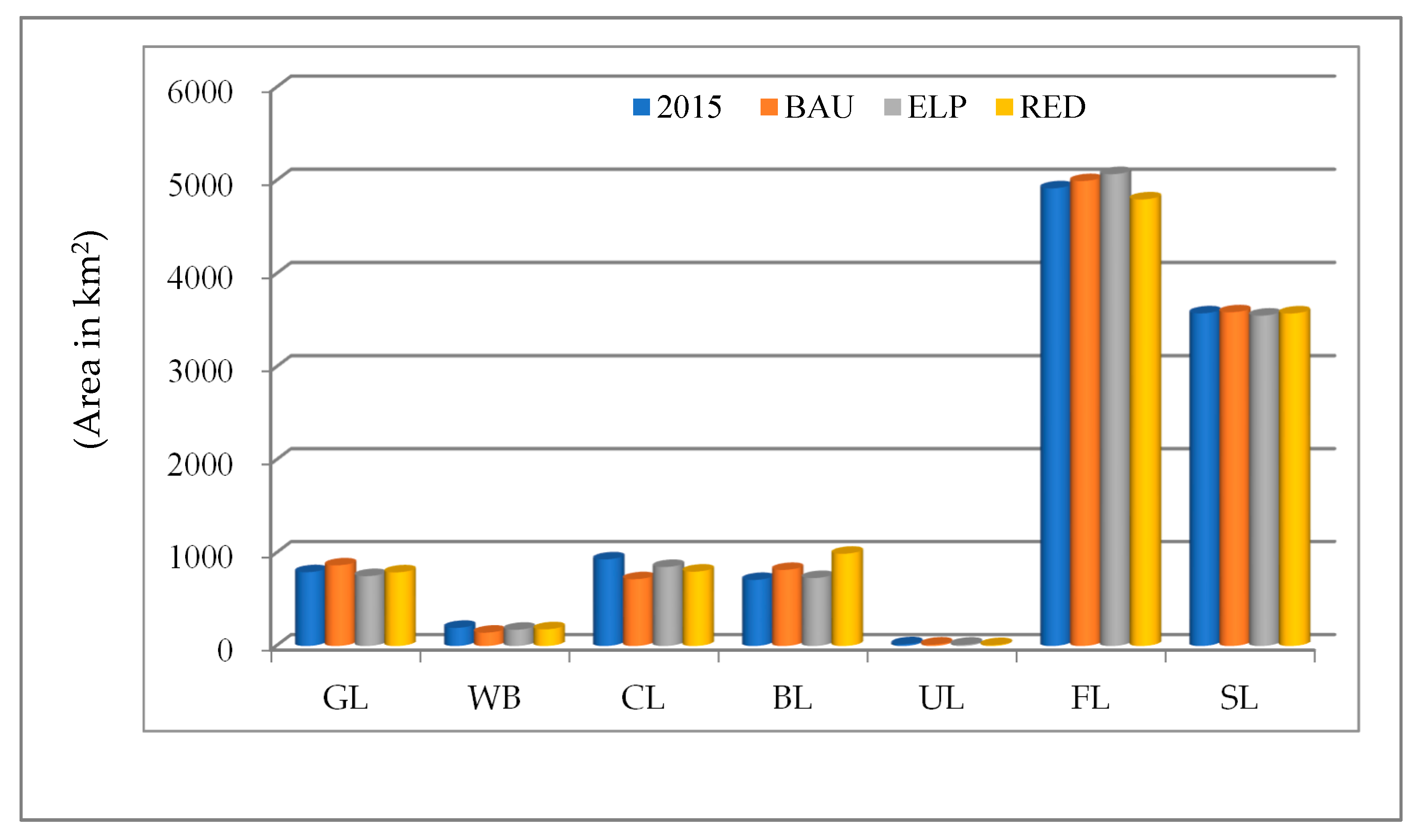
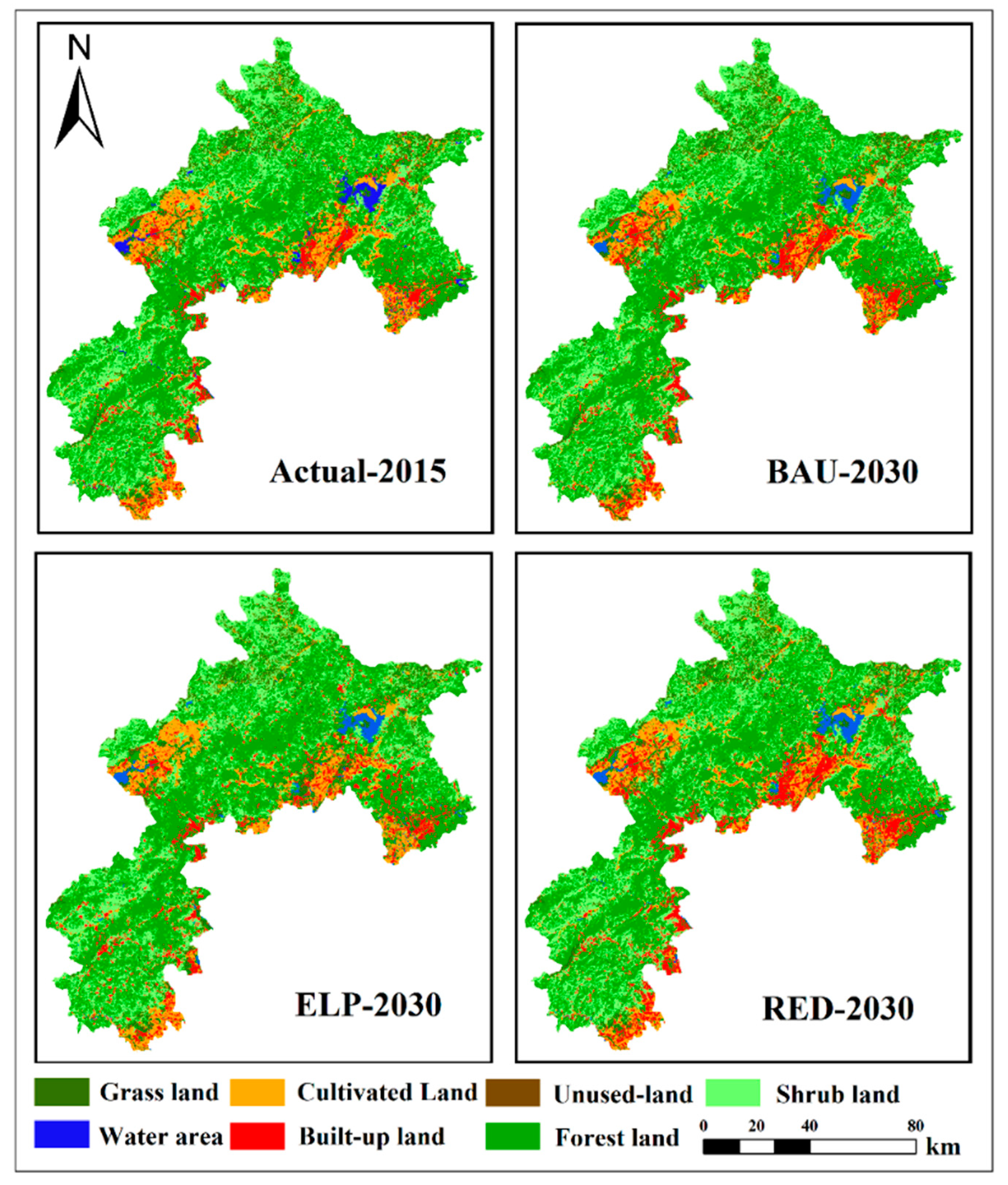
3.1. Changes in Land Use under Different Scenarios

Throughout the duration of the study, most land in the ecological conservation area was predicted to remain covered by forest and shrub land; however, several transitions were predicted among land-use types under all three scenarios (Table 2; Figure 2). From 2015 to 2030, land-use-type change is mainly characterized by built-up land expansion and loss of cultivated, water body, and unused land. Cultivated and built-up land changes are ranked differently according to the proportion under different scenarios. As expected, the RED scenario presents the greatest built-up land expansion (+2.52%), which is much higher than those predicted under the BAU and ELP scenarios (+0.96% and +0.18%, respectively). The importance of land-use planning and other regulations is clear when comparing the land-use projections for the ELP and BAU scenarios. For example, under the ELP scenario, the total area of forest land is projected to increase by 152.38 km2 (+1.36%), but the extent of built-up land and water body remain relatively stable (+20.34 and -20.55 km2, respectively), and cultivated land decreases relatively little (-81.39 km2).
The increase in built-up land occurs at the expense of all other land-use types from 2015 to 2030, under the RED scenario, but especially from the conversion of cultivated land and water bodies (Table 3 and Figure 3). Under the BAU and RED scenarios, the expansion of built-up land is derived from the conversion of 134 km2 of cultivated land alone, which contributes to the decline of cultivated land from 8.36% to 6.44% and 7.17%, respectively. Under the ELP scenario, forest land expands from 44.14% to 45.50%, largely from conversions from shrub land, grassland, and cultivated land. However, shrub land declines only slightly under the ELP scenario, as more than 1000 km2 of forest land and 231.66 km2 grassland area are converted to shrub land.

3.2. Future Changes in Ecosystem Services

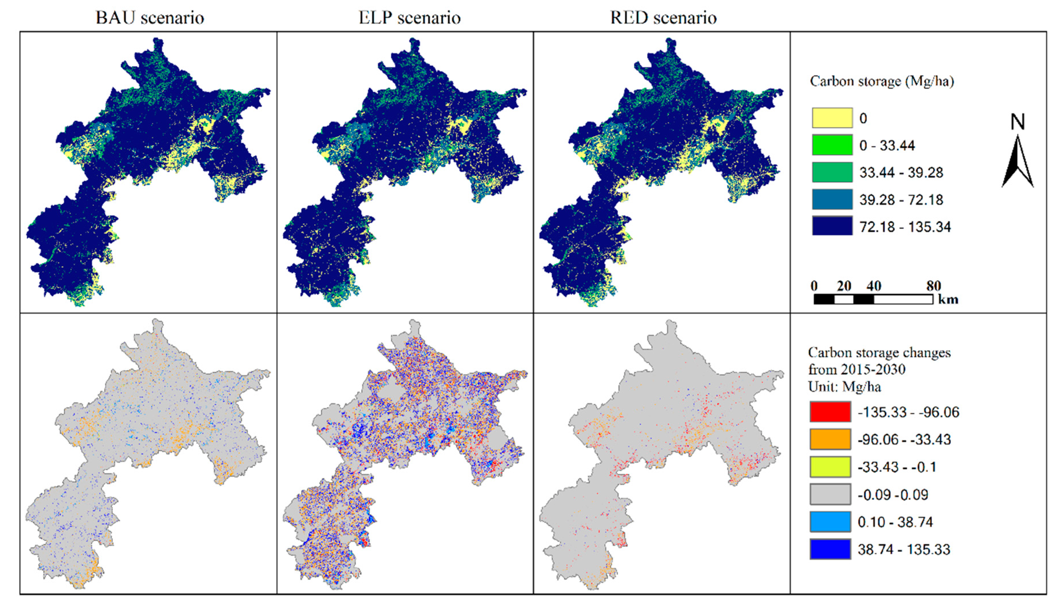
3.2.1. Carbon Storage

The total carbon storage was 98.92 Tg in 2015, and was predicted to decrease to 96.74 Tg in 2030, under the RED scenario—primarily caused by rapid urban encroachment into cultivated and forest land (Supplementary Table S11). The ELP scenario was predicted to result in the highest amount of total carbon storage (100.24 Tg), due to grassland, shrub land, and forest land expansion (+1.27 Tg). Forest land presents the highest carbon storage capacity, and expected 2030 carbon storage values of 65.42, 66.80, and 63.75 Tg were predicted under the BAU, ELP, and RED scenarios, respectively (Supplementary Table S7). The transition from forest to built-up land leads to the greater loss of carbon storage under the ELP and RED scenarios, respectively (Supplementary Table S11). Furthermore, carbon storage growth was distributed predominantly on the periphery of grassland, cultivated land, and shrub land due to the expansion of forest land and shrub land (Figure 4).

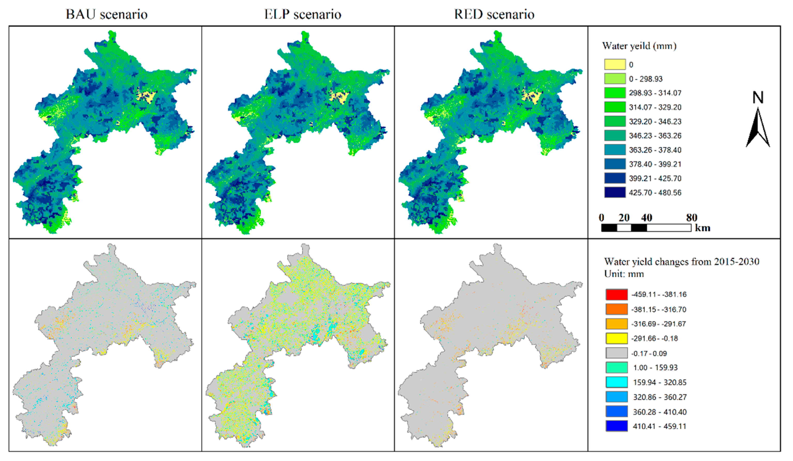
3.2.2. Flood Regulation

The total flood regulation capacity was predicted to decrease from the 2015 baseline (350.37 ten million m3) to 2030, under the BAU, ELP, and RED scenarios (Supplementary Table S8). In 2030, the total predicted amount of water yield under RED scenario will have the highest totaling water yield (totaling 352.26 ten million m3), which is +1.89 ten million m3 more than 2015 and has the lowest flood regulation ability (Supplementary Table S8). The transition from cultivated land and forest land to built-up land triggered increased water yield under the RED scenario. The ELP scenario will be + 0.12 ten million m3 compared to 2015 (totaling 350.49 ten million m3), due to the transition from grassland, cultivated land, and shrub land to forest land. Among all of the land-use types, the flood regulation of built-up land is projected to have the highest increase, from 26.83 ten million m3 to 36.81 ten million m3 (9.98 ten million m3) by 2030, under the RED scenario, due to the increase in built-up land area and low flood regulation capacity (Supplementary Tables S8 and S11). The changes of flood regulation are mainly distributed in the transition zones between forest and shrub land, under the ELP scenario, because of the high runoff coefficient of built-up land and cultivated land (Figure 5). Under the other two scenarios, flood-regulation changes are mainly distributed around cities, cultivated land, and water bodies.

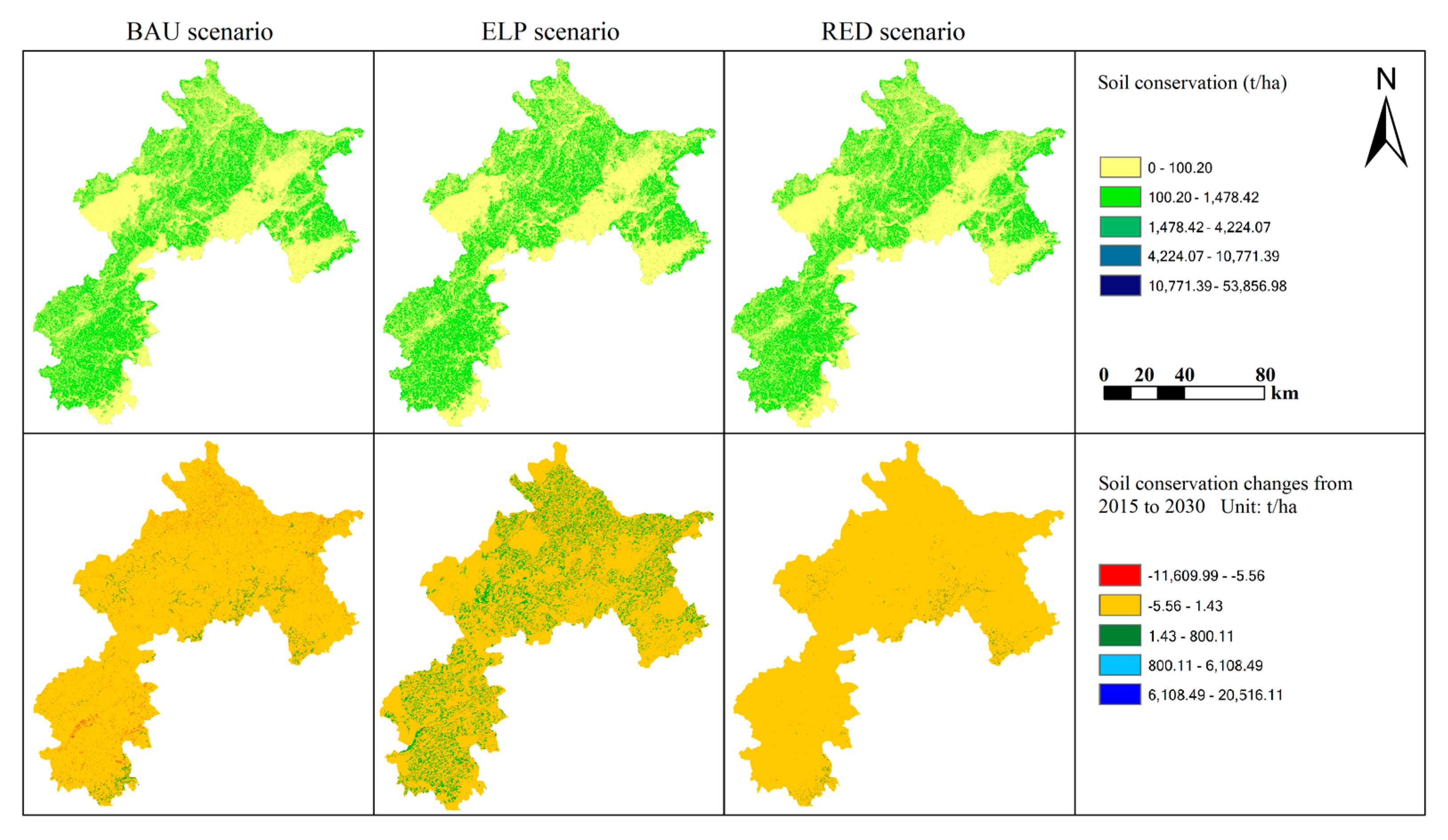
3.2.3. Soil Conservation

The predicted soil conservation exhibited disparate patterns under the BAU compared to ELP and RED scenarios (Supplementary Table S9). Under the BAU scenario, soil conversion is predicted to decrease from 246.86 ten million tons in 2015 to 246.74 ten million tons in 2030, a decline of 0.12 ten million tons, due to the conversion from cultivated land to grass land and forest land to shrub land (Supplementary Table S11). The ELP and RED scenarios predict an increase of 3.4 ten million tons and 1.88 ten million tons, respectively, which could be attributed to the transition from cultivated land and forest to built-up land (Supplementary Table S11). Under the ELP scenario, the soil conservation of shrub land showed the greatest decline—from 97.12 ten million tons to 87.94 ten million tons; however, the large conversion from shrub land to forest land offsets this deficiency. Despite the overall increase in soil conservation in 2030, under the RED scenario, several spatial areas experience a decline in soil conservation due mainly to a reduction of forest land, cultivated land, and water bodies (Figure 6). Among all of the land-use types, shrub land presents the highest soil conservation capacity, with an average quantity of 4.80 t/km2 in 2015 and 5.54 t/km2 in 2030.

3.3. Trade-Offs and Synergies among Ecosystem Services

We performed correlation analyses between pairs of ES, to explore the trade-offs and synergies in the ecological conservation area during the period from 2015 to 2030 (Table 4 and Supplementary Table S10). The trade-offs and synergies were identified by the correlation coefficient. Carbon storage (CS) and soil conservation (SC) would be positively correlated with each other throughout the period from 2015 to 2030, indicating the existence of synergistic effect between these two ecosystem services. At the same time, it also suggests the high capacity of forest and shrub land in sequestering carbon and regulating water runoff in the ecological conservation area. The correlation between carbon storage and soil conservation presented the strongest under the ELP scenario, and the correlation coefficient was 0.642. The positive relationship between soil conservation (SC) and flood regulation (FR) from 2015 to 2030, under the ELP scenario, respectively, proved the existence of synergies. In addition, carbon storage was not correlated with flood regulation in 2015, but these two ecosystem services would be positively correlated under the BAU, ELP, and RED scenarios. This implies that ecological land, including forest land and shrub land, will become increasingly important in regulating water balance in the future.

4. Discussion

4.1. Response of Ecosystem Services to Land-Use Changes

In this study, we found major changes in land-use analysis over the period from 2015 to 2030, under three alternative scenarios, including rapid expansion of built-up land, increase of forest and grassland, and sharp declines in cultivated land, water bodies, and unused land. The impacts of these changes on ecosystem services vary in direction and magnitude under different development scenarios. For instance, the expansion of built-up land can result in decreased supply to multiple ecosystem services—carbon storage and flood regulation [54,55], as our results show during the conversion from forest and cultivated land to built-up land under the BAU and RED scenario. Generally, ecosystems changing from high vegetation cover to low vegetation cover will exhibit decreased carbon storage and water conservation [14,56,57]. When compared with other land-use types, forest land was the major carbon sink. It also suggests that the necessity of ecological protection projects in our study area. However, we also find that the conversion of shrub land and unused land to built-up land can lead to beneficial effects, such as stabilization of sand and reduction of soil erosion, as has been previously reported [32,58].
The flood regulation and soil conservation provided by different land-use classes are associated with natural and physical conditions, such as climate, soil, and geology. For instance, our result shows that the conversion from forest land to grassland or shrub land generally resulted in a decrease in carbon storage, soil conservation, and flood regulation. On the one hand, due to the lower plant density and root depth, grassland and shrub ecosystems have less regulating capacity on rainfall than forest ecosystems, so the lower water percolating capacity of grassland and shrub land results in a relatively low flood regulation. In addition, previous researches have shown that vegetation plays an important role in controlling soil erosion by intercepting rainfall, increasing infiltration, and stabilizing the soil [32]. On the other hand, forest land going to grassland will lead to increased soil erosion because of the steep terrain and heavy rainfall, which are prone to landslides, mudslides, and other geological hazards in the mountain zone, and therefore threaten grazing, tourism, etc. [59,60]. Therefore, soil erosion is more likely to occur under the BAU and RED scenarios. On the contrary, the conversion of grassland and cultivated land to forest land resulted in a greater increase in carbon storage and soil conservation, especially under the ELP scenario. This can be explained that the strict spatial regulations of the ELP scenario that forbid the conversion of the Miyun reservoir and 21 nature reserves, according to the “Beijing’s General Urban Planning (2016–2035)”.
Our study also shows that, in addition to the differential ES provision, land-use changes will affect trade-offs and synergies among ES. For example, gains in soil conservation typically result in increased flood regulation in 2015 and 2030 under the ELP scenario. It could be explained that forest cover accounting for the largest proportion under the ELP scenario will protect soil surfaces from rainfall and promote flood regulation increase, but possibly lead to water scarcity. In addition, when shrub land is converted to grassland, flood regulation shows a decrease trend, in contrast with carbon storage and soil conservation, consistent with [61]. Therefore, the conversion between land-use types in the ecological conservation area must be managed carefully. Forest has played an important role in local and regional climate regulation and water conservation [62]. Thus, although urban expansion may boost the regional economy, the conversion of forest land to built-up land will likely lead to great losses of climate and flood regulation services. Therefore, the study of the correlations between land-use changes and ES trade-offs warrant further investigation [63,64].

4.2. Strategies and Implications

We propose the maximizing ecological benefits (ELP) scenario for the ecological conservation area. In comparison to the other two scenarios, we predict that the BAU scenario presents a number of undesirable environmental outcomes. Water reserves, natural reserves, and several national forest parks are forbidden to convert to other land uses under the ELP and RED scenarios in compliance with ecological protection plants. Our results indicate that the expansion of built-up land will be effectively controlled, with less natural or semi-natural ecosystems being converted to built-up land under the ELP scenario. The RED scenario showed an increase in soil conservation, but decreases in carbon storage and flood regulation compared to the BAU scenario. These trade-offs are the issues that urban planners face as they chart out a future for growing cities. The ELP scenario should be a future priority because it takes into account the land needed to meet the multitude of resources and growing population demands, as proposed in the “Beijing’s General Urban Planning (2016–2035)”. Therefore, we suggest that the People’s Government of Beijing Municipality should strengthen the implementation of natural resources protection planning and spatial control, to effectively alleviate ecosystem degradation.
Our study has identified hotspots of ecosystem-service gains and losses that respond to land-use changes, allowing us to proscribe cost-effective land-use spatial regulations for maintaining and enhancing ecosystem services. We further propose four major strategies that may be used as guidelines for improving ecosystem services in the ecological conservation area. First, and most importantly, more efficient use of current urban land resources should be adopted, such as more compact buildings and redevelopment of discarded factories, as suggested by [9,16]. Second, high-quality cultivated land, especially basic farmland, should be strictly protected from urban expansion, to ensure adequate food supply. Third, trees, especially along primary roads, should be enhanced, as the increase in forest cover will promote the regional spatial balance of carbon storage in these areas in the future [65]. Finally, we must improve the utilization of water resources; most precipitation is transported into urban sewers and cannot be easily used by human beings [66,67]. In conclusion, through wise land-use management, the win-win development patterns of natural ecosystems and socioeconomic systems can be realized in the future.

4.3. Strengths and Limitations

As mentioned above, the main components of our study were land-use simulation and ecosystem services evaluation. Our methodology provides a straightforward and flexible way to explore possible implications of land-use change for ecosystem services under future land-use conditions. Another strength is that these results will inform researchers and policymakers as they draft appropriate measures to better adapt to different future scenarios [68]. However, some limitations always exist in future land-use simulation, and this is true for our analysis of the ecological conservation area. For instance, the GeoSOS-FLUS model transition rules (referring primarily to the conversion cost and the well-trained ANN model) are assumed to be unchanged during the simulation process, while these rules may change at a certain time in the future (e.g., 30 or 50 years), in the real world [69].
The InVEST model applied here has been widely used for assessing ecosystem services across multiple time scales [56,70,71]; however, we also recognize its modeling and data limitations. Firstly, the results for evaluating ES are dependent on the land-use classifications used. Here we classify land use into seven broad classes, in which all types of minor lands are assumed homogeneous. For example, carbon storage capacity within a forest landscape is affected by temperature, elevation, rainfall, and forest age, which were not captured by our classification scheme. Secondly, although we used land-use maps derived from 30 m resolution remote-sensing images, other data, including soil, precipitation, and temperature were available only at 1000 m resolution, which increases the uncertainty of ecosystem service evaluation. Thirdly, the “Annual Water Yield” module is based on annual averages, which neglect extrema and does not consider sub-annual patterns of water delivery timing [72]. Finally, given the simplicity of the InVEST model and small number of parameters, the output results of the “sediment delivery ratio” module are very sensitive to most input parameters [73]. Therefore, the errors of the empirical parameters of the USLE equation will have a great effect on our predictions.
The purpose of this study was to explore the impacts of land-use change on ecosystem services under different scenarios, which can provide information for the formulation of land-use policy. Given this objective, climate remains constant from 2015 to 2030, leaving land-use change as the sole driver affecting changes in ecosystem services. Assessing the impact of climate and land-use changes on ecosystem services is valuable, as they have been identified as the two main factors driving the provision of ES and trade-offs [74]. Among them, climate change impacts on ES by modifying the biophysical processes of ecosystems. Although there have been some studies exploring the relative importance of land use and climate on ES [70,75,76], how the different climate models incorporate land-use policies is still a challenge in the future. Therefore, our next work will focus on the relative and combined effects of climate and land-use changes on ES and trade-offs among multiple ES under different scenarios in the future.

5. Conclusions

In this study, we explored how land-use changes would affect ecosystem services, including carbon storage, flood regulation, and soil conservation, from 2015 to 2030, under three different scenarios. According to our results, the significant increase of built-up land is mainly at the expense of the water bodies and cultivated land in 2030, under the BAU and RED scenarios. The ELP scenario would show the largest increase in forest land, and the change of cultivated land and built-up land is relatively stable compared with the other two scenarios, due to the strict protection policy on ecological land. As a result, the ELP scenario would show the highest amount of carbon storage, flood regulation, and soil conservation. The cultivated land and forest land converted to built-up land would promote soil conservation, but trigger greater loss of carbon storage and flood regulation capacity. We also found trade-offs or synergies among ecosystem services in which carbon storage would show significant positive correlation with soil conservation from 2015 to 2030. Based on these findings, we propose four major land-use strategies, including fully utilizing urban land, farmland protection, tree planting, and utilization of water resources to achieve sustainable use of ecosystem services in the ecological conservation area.

Supplementary Materials

The following are available online at https://www.mdpi.com/1999-4907/11/5/584/s1. Figure S1: Land-use maps of 2000 for the ecological conservation area in Beijing, China. Table S1: Description of land-use types. Table S2: Driving factors of land-use change. Table S3: Conversion cost matrix from 2000 to 2015 (km2). Table S4: Input data on carbon stored in each of the four fundamental pools for each LULC class in the InVEST 3.8.0 model (Mg/ha). Table S5: Input data for each LULC class in the InVEST 3.8.0 water yield model. Table S6: Input data for each LULC class in the InVEST 3.8.0 sediment delivery ratio model. Table S7: Carbon storage (CS) for each land-use type from baseline, in 2030 under the BAU, ELP, and RED scenarios (Tg). Table S8: Water yield (WY) for each land-use type from baseline, in 2030, under the BAU, ELP, and RED scenarios (million m3). Table S9: Soil conservation (CS) for each land-use type from baseline, in 2030, under the BAU, ELP, and RED scenarios (million ton). Table S10: Correlation among three ecosystem services for each scenario. Table S11, Ecosystem service (ES) change matrix driven by per-unit land-use transitions of the main land-use types, from 2015 to 2030, under the BAU, ELP, and RED scenarios.

Author Contributions

Conceptualization, H.H.; methodology, Z.L.; software, Z.L.; investigation, H.H. and Z.L.; resources, X.C.; data curation, X.C.; validation, Z.L.; writing—original draft preparation, Z.L.; writing—review and editing, X.C.; project administration, H.H.; funding acquisition, H.H. All authors have read and agreed to the published version of the manuscript.

Funding

This research was funded by the National Key Research and Development Program of China (No. 2019YFA0607304).

Conflicts of Interest

The authors declare no conflict of interest.

References

  1. Costanza, R.; D’Arge, R.; De Groot, R. The value of the world’s ecosystem services and natural capital. Nature 1997, 387, 253–260. [Google Scholar] [CrossRef]
  2. Millennium Ecosystem Assessment (MEA). Ecosystems and Human Well-Being: Synthesis; Island Press: Washington, DC, USA, 2005. [Google Scholar]
  3. La Notte, A.; D’Amato, D.; Mäkinen, H.; Paracchini, M.L.; Liquete, C.; Egoh, B.; Geneletti, D.; Crossman, N.D. Ecosystem services classification: A systems ecology perspective of the cascade framework. Ecol. Ind. 2017, 74, 392–402. [Google Scholar] [CrossRef] [PubMed]
  4. Foley, J.A.; Defries, R.S.; Asner, G.P.; Barford, C.; Bonan, G.; Carpenter, S.R.; Chapin, F.S.; Coe, M.T.; Daily, G.C.; Gibbs, H.K. Global Consequences Land Use. Science 2005, 309, 570–574. [Google Scholar] [CrossRef] [Green Version]
  5. Defries, R.S.; Foley, J.A.; Asner, G.P. Land-use choices: Balancing human needs and ecosystem function. Front. Ecol. Environ. 2004, 2, 249–257. [Google Scholar] [CrossRef]
  6. He, C.; Liu, Z.; Tian, J.; Ma, Q. Urban expansion dynamics and natural habitat loss in China: A multiscale landscape perspective. Glob. Change. Biol. 2014, 20, 2886–2902. [Google Scholar] [CrossRef] [PubMed]
  7. Lawler, J.J.; Lewis, D.J.; Nelson, E.; Plantinga, A.J.; Polasky, S.; Withey, J.C.; Helmers, D.P.; Martinuzzi, S.; Pennington, D.; Radeloff, V.C. Projected land-use change impacts on ecosystem services in the United States. Proc. Natl. Acad. Sci. USA 2014, 111, 7492–7497. [Google Scholar] [CrossRef] [PubMed] [Green Version]
  8. Nkonya, E.; Anderson, W.; Kato, E.; Koo, J.; Mirzabaev, A.; Braun, J.V.; Meyer, S. Global cost of Land degradation. In Title of the Economics of Land Degradation and Improvement-A Global Assessment for Sustainable Development; Nkonya, E., Mirzabaev, A., von Braun, J., Eds.; Springer: Cham, Switzerland, 2016; pp. 117–166. [Google Scholar]
  9. Wu, Y.; Tao, Y.; Yang, G.; Ou, W.; Pueppke, S.; Sun, X.; Chen, G.; Tao, Q. Impact of land use change on multiple ecosystem services in the rapidly urbanizing kunshan city of china: Past trajectories and future projections. Land Use Policy 2019, 85, 419–427. [Google Scholar] [CrossRef]
  10. Rodríguez, J.P.; Beard, T.D., Jr.; Bennett, E.M.; Cumming, G.; Cork, S.; Agard, J.; Dobson, A.; Peterson, G. Trade-offs across space, time, and ecosystem services. Ecol. Soc. 2006, 11, 16. [Google Scholar] [CrossRef] [Green Version]
  11. Roopsind, A.; Caughlin, T.T.; Hout, P.V.D.; Arets, E.; Putz, F.E. Trade-offs between carbon stocks and timber recovery in tropical forests are mediated by logging intensity. Glob. Chang. Biol. 2018, 24, 2862–2874. [Google Scholar] [CrossRef] [Green Version]
  12. Blumstein, M.; Thompson, J.R. Land-use impacts on the quantity and configuration of ecosystem service provisioning in Massachusetts, USA. J. Appl. Ecol. 2015, 52, 1009–1019. [Google Scholar] [CrossRef]
  13. Lin, W.; Xu, D.; Guo, P.; Wang, D.; Li, L.; Gao, J. Exploring variations of ecosystem service value in Hangzhou Bay Wetland, Eastern China. Ecosyst. Serv. 2019, 37, 100944. [Google Scholar] [CrossRef]
  14. Wang, Z.; Mao, D.; Li, L.; Jia, M.; Dong, Z.; Miao, Z.; Ren, C.; Song, C. Quantifying changes in multiple ecosystem services during 1992-2012 in the Sanjiang Plain of China. Sci. Total Environ. 2015, 514, 119–130. [Google Scholar] [CrossRef] [PubMed]
  15. Vaighan, A.A.; Talebbeydokhti, N.; Bavani, A.M. Assessing the impacts of climate and land use change on streamflow, water quality and suspended sediment in the Kor River Basin, Southwest of Iran. Environ. Earth Sci. 2017, 76, 1–18. [Google Scholar] [CrossRef]
  16. Clough, Y.; Krishna, V.V.; Corre, M.D.; Darras, K.; Denmead, L.H.; Meijide, A.; Moser, S.; Musshoff, O.; Steinebach, S.; Veldkamp, E. Land-use choices follow profitability at the expense of ecological functions in Indonesian smallholder landscapes. Nat. Commun. 2016, 7, 1–12. [Google Scholar] [CrossRef]
  17. Wang, Y.; Li, X.; Zhang, Q.; Li, J.; Zhou, X. Projections of future land use changes: Multiple scenarios-based impacts analysis on ecosystem services for Wuhan city, China. Ecol. Indic. 2018, 94, 430–445. [Google Scholar] [CrossRef]
  18. Gong, J.; Liu, D.; Zhang, J.; Xie, Y.; Cao, E.; Li, H. Tradeoffs/synergies of multiple ecosystem services based on land use simulation in a mountain-basin area, western China. Ecol. Indic. 2019, 99, 283–293. [Google Scholar] [CrossRef]
  19. Dymond, J.R.; Ausseil, A.G.; Djanibekov, N.; Lamers, J.P.A. How attractive are short-term CDM forestations in arid regions? The case of irrigated cropland in Uzbekistan. For. Policy Econ. 2012, 21, 108–117. [Google Scholar]
  20. Xu, Y.; Tang, H.P.; Wang, B.J.; Chen, J. Effects of land-use intensity on ecosystem services and human well-being: A case study in Huailai County, China. Environ. Earth Sci. 2016, 75, 415–425. [Google Scholar] [CrossRef]
  21. Pereira, H.M.; Navarro, L.M.; Santos Martins, I. Global biodiversity change: The bad, the good, and the unknown. Ann. Rev. Environ. Resour. 2012, 37, 25–50. [Google Scholar] [CrossRef] [Green Version]
  22. Wang, L.; Zheng, H.; Wen, Z.; Liu, L.; Robinson, B.E.; Li, R.; Li, C.; Kong, L. Ecosystem service synergies/trade-offs informing the supply-demand match of ecosystem services: Framework and application. Ecosyst. Serv. 2019, 37, 100939. [Google Scholar] [CrossRef]
  23. Zhang, D.; Huang, Q.; He, C.; Yin, D.; Liu, Z. Planning urban landscape to maintain key ecosystem services in a rapidly urbanizing area: A scenario analysis in the Beijing-Tianjin-Hebei urban agglomeration, China. Ecol. Indic. 2019, 96, 559–571. [Google Scholar] [CrossRef]
  24. Dong, N.; You, L.; Cai, W.; Li, G.; Lin, H. Land use projections in China under global socioeconomic and emission scenarios: Utilizing a scenario-based land-use change assessment framework. Glob. Environ. Chang. 2018, 50, 164–177. [Google Scholar] [CrossRef]
  25. Sun, Y.; Liu, S.; Dong, Y.; An, Y.; Shi, F.; Dong, S.; Liu, G. Spatio-temporal evolution scenarios and the coupling analysis of ecosystem services with land use change in China. Sci. Total Environ. 2019, 681, 211–225. [Google Scholar] [CrossRef] [PubMed]
  26. Shoemaker, D.A.; BenDor, T.K.; Meentemeyer, R.K. Anticipating trade-offs between urban patterns and ecosystem service production: Scenario analyses of sprawl alternatives for a rapidly urbanizing region. Comput. Environ. Urban. 2018, 74, 114–125. [Google Scholar] [CrossRef]
  27. Pickard, B.R.; Van Berkel, D.; Petrasova, A.; Meentemeyer, R.K. Forecasts of urbanization scenarios reveal trade-offs between landscape change and ecosystem services. Landsc. Ecol. 2017, 32, 617–634. [Google Scholar] [CrossRef]
  28. Costanza, R.; Ruth, M. Using dynamic modeling to scope environmental problems and build consensus. Environ. Manag. 1998, 22, 183–195. [Google Scholar] [CrossRef]
  29. Verburg, P.H.; Schot, P.P.; Dijst, M.J.; Veldkamp, A. Land use change modelling: Current practice and research priorities. GeoJournal 2004, 61, 309–324. [Google Scholar] [CrossRef]
  30. Yang, Z.C.; Zhou, L.D.; Sun, D.F.; Li, H.; Yu, M. Proposal for Developing Carbon Sequestration Economy in Ecological Conservation Area of Beijing. Adv. Mater. Res. 2012, 524, 3424–3427. [Google Scholar] [CrossRef]
  31. Wang, J.; Lv, K.; Zhang, Y. Study on Adjusting and Optimizing the Forest Resources Structure in Beijing Ecological Conservation Area. For. Resour. Manag. 2009, 2, 66–69. [Google Scholar]
  32. Sun, X.; Lu, Z.; Li, F.; Crittenden, J.C. Analyzing spatio-temporal changes and trade-offs to support the supply of multiple ecosystem services in Beijing, China. Ecol. Indic. 2018, 94, 117–129. [Google Scholar] [CrossRef]
  33. Muller, M.R.; Middleton, J. A Markov model of land-use change dynamics in the Niagara Region, Ontario, Canada. Landsc. Ecol. 1994, 9, 151–157. [Google Scholar]
  34. Liu, X.; Liang, X.; Li, X.; Xu, X.; Ou, J.; Chen, Y.; Li, S.; Wang, S.; Pei, F. A future land use simulation model (FLUS) for simulating multiple land use scenarios by coupling human and natural effects. Landsc. Urban Plan. 2017, 168, 94–116. [Google Scholar] [CrossRef]
  35. Bai, Y.; Wong, C.P.; Jiang, B.; Hughes, A.; Wang, M.; Wang, Q. Developing China’s Ecological Redline Policy using ecosystem services assessments for land use planning. Nat. Commun. 2018, 9, 1–13. [Google Scholar] [CrossRef] [PubMed] [Green Version]
  36. Kamusoko, C.; Aniya, M.; Adi, B.; Manjoro, M. Rural sustainability under threat in Zimbabwe Simulation of future land use/cover changes in the Bindura district based on the Markov-cellular automata model. Appl. Geogr. 2009, 29, 435–447. [Google Scholar] [CrossRef]
  37. Fu, X.; Wang, X.; Yang, Y.J. Deriving suitability factors for CA-Markov land use simulation model based on local historical data. J. Environ. Manag. 2017, 206, 10–19. [Google Scholar] [CrossRef]
  38. Baltzer, H. Markov chain models for vegetation dynamics. Ecol. Model. 2000, 126, 139–154. [Google Scholar]
  39. Li, X.; Yeh, A.G. Neural-network-based cellular automata for simulating multiple land use changes using GIS. Int. J. Geogr. Inf. Sci. 2002, 16, 323–343. [Google Scholar] [CrossRef]
  40. Wu, F.; Webster, C.J. Simulation of land development through the integration of cellular automata and multicriteria evaluation. Environ. Plan. B 1998, 25, 103–126. [Google Scholar] [CrossRef]
  41. Van Asselen, S.; Verburg, P.H. Land cover change or land-use intensification: Simulating land system change with a global-scale land change model. Glob. Chang. Biol. 2013, 19, 3648–3667. [Google Scholar] [CrossRef]
  42. Pontius, R.G.; Boersma, W.; Castella, J.; Clarke, K.; de Nijs, T.; Dietzel, C.; Verburg, P.H. Comparing the input, output, and validation maps for several models of land change. Ann. Regional. Sci. 2008, 42, 11–137. [Google Scholar] [CrossRef] [Green Version]
  43. Chen, Y.; Liu, X.; Li, X. Calibrating a Land Parcel Cellular Automaton (LPCA) for urban growth simulation based on ensemble learning. Int. J. Geogr. Inf. Sci. 2017, 31, 2480–2504. [Google Scholar] [CrossRef]
  44. Li, X.; Chen, G.; Liu, X.; Liang, X.; Xu, X.; Wang, S.; Chen, Y.; Pei, F. A new global land-use and land-cover change product at a 1-km resolution for 2010 to 2100 based on human–environment interactions. Ann. Am. Assoc. Geogr. 2017, 107, 1040–1059. [Google Scholar] [CrossRef]
  45. Kriegler, E.; Edmonds, J.; Hallegatte, S.; Ebi, K.L.; Kram, T.; Riahi, K.; Winkler, H.; Van Vuuren, D.P. A new scenario framework for climate change research: The concept of shared climate policy assumptions. Clim. Chang. 2014, 122, 401–414. [Google Scholar] [CrossRef] [Green Version]
  46. Calvin, K.; Bond-Lamberty, B.; Clarke, L.; Edmonds, J.; Eom, J.; Hartin, C.; Kim, S.; Kyle, P.; Link, R.; Moss, R.; et al. SSP4: A world of deepening inequality. Glob. Environ. Chang. 2017, 42, 284–296. [Google Scholar] [CrossRef] [Green Version]
  47. Schirpke, U.; Kohler, M.; Leitinger, G.; Fontana, V.; Tasser, E.; Tappeiner, U. Future impacts of changing land-use and climate on ecosystem services of mountain grassland and their resilience. Ecosyst. Serv. 2017, 26, 79–94. [Google Scholar] [CrossRef] [PubMed]
  48. Sharps, K.; Masante, D.; Thomas, A.; Jackson, B.; Redhead, J.; May, L.; Prosser, H.; Cosby, B.; Emmett, B.; Jones, L. Comparing strengths and weaknesses of three ecosystem services modelling tools in a diverse UK river catchment. Sci. Total Environ. 2017, 584, 118–130. [Google Scholar] [CrossRef] [PubMed] [Green Version]
  49. Sharp, R.; Tallis, H.T.; Ricketts, T.; Guerry, A.D.; Wood, S.A.; Chaplin-Kramer, R.; Nelson, E.; Ennaanay, D.; Wolny, S.; Olwero, N.; et al. InVEST 3.8.0 User’s Guide; The Natural Capital Project, Stanford University, University of Minnesota, The Nature Conservancy, and World Wildlife Fund: Minneapolis, MN, USA; Available online: http://releases.naturalcapitalproject.org/invest-userguide/latest/#supporting-tools (accessed on 18 January 2020).
  50. Fu, B.P. On the calculation of the evaporation from land surface (in Chinese). J. Atmos. Sci. 1981, 5, 23–31. [Google Scholar]
  51. Zhang, L.; Hickel, K.; Dawes, W.R.; Chiew, F.H.S.; Western, A.W.; Briggs, P.R. A rational function approach for estimating mean annual evapotranspiration. Water Resour. Res. 2004, 40. [Google Scholar] [CrossRef]
  52. Kareiva, P.; Tallis, H.; Ricketts, T.H.; Daily, G.C.; Polasky, S. Natural Capital: Theory and Practice of Mapping Ecosystem Services; Oxford University Press: Oxford, UK, 2011; pp. 3–128. [Google Scholar]
  53. Ouyang, Z.Y.; Zheng, H.; Xiao, Y.; Polasky, S.; Liu, J.; Xu, W.; Wang, Q.; Zhang, L.; Rao, E.; Jiang, L. Improvements in ecosystem services from investments in natural capital. Science 2016, 352, 1455–1459. [Google Scholar] [CrossRef]
  54. Haas, J.; Ban, Y.F. Urban growth and environmental impacts in Jing-Jin-Ji, the Yangtze, River Delta and the Pearl River Delta. Int. J. Appl. Earth Obs. 2014, 30, 42–55. [Google Scholar] [CrossRef]
  55. Zhang, D.; Huang, Q.X.; He, C.Y.; Wu, J.G. Impacts of urban expansion on ecosystem services in the Beijing-Tianjin-Hebei urban agglomeration, China: A scenario analysis based on the Shared Socioeconomic Pathways. Resour. Conserv. Recycl. 2017, 125, 115–130. [Google Scholar] [CrossRef]
  56. Gao, J.; Li, F.; Gao, H.; Zhou, C.; Zhang, X. The impact of land-use change on water-related ecosystem services: A study of the Guishui River Basin, Beijing, China. J. Clean. Prod. 2017, 163, S148–S155. [Google Scholar] [CrossRef]
  57. López-Moreno, J.I.; Vicente-Serrano, S.M.; Moran-Tejeda, E.; Zabalza, J.; Lorenzo-Lacruz, J.; García-Ruiz, J.M. Impact of climate evolution and land use changes on water yield in the ebro basin. Hydrol. Earth Syst. Sci. 2011, 15, 311–322. [Google Scholar] [CrossRef] [Green Version]
  58. Lyu, R.; Zhang, J.; Xu, M.; Li, J. Impacts of urbanization on ecosystem services and their temporal relations: A case study in Northern Ningxia, China. Land Use Policy 2018, 77, 163–173. [Google Scholar] [CrossRef]
  59. Lü, Y.; Fu, B.; Feng, X.; Zeng, Y.; Liu, Y.; Chang, R.; Sun, G.; Wu, B. A policy-driven large scale ecological restoration: Quantifying ecosystem services changes in the loess plateau of China. PLoS ONE 2012, 7, 1–10. [Google Scholar] [CrossRef]
  60. Fu, B.; Liu, Y.; Lü, Y.; He, C.; Zeng, Y.; Wu, B. Assessing the soil erosion control service of ecosystems change in the Loess Plateau of China. Ecol. Complex. 2011, 8, 284–293. [Google Scholar] [CrossRef]
  61. Wang, X.; Bennett, J. Policy analysis of the conversion of cropland to forest and grassland program in China. Environ. Econ. Policy Stud. 2008, 9, 119–143. [Google Scholar] [CrossRef]
  62. Turner, K.G.; Odgaard, M.V.; Bøcher, P.K.; Dalgaard, T.; Svenning, J.-C. Bundling ecosystem services in Denmark: Trade-offs and synergies in a cultural landscape. Landsc. Urban Plan. 2014, 125, 89–104. [Google Scholar] [CrossRef]
  63. Bennett, E.M.; Peterson, G.D.; Gordon, L.J. Understanding relationships among multiple ecosystem services. Ecol. Lett. 2009, 12, 1394–1404. [Google Scholar] [CrossRef]
  64. Jia, X.; Fu, B.; Feng, X.; Hou, G.; Liu, Y.; Wang, X. The tradeoff and synergy between ecosystem services in the grain-for-green areas in Northern Shaanxi, China. Ecol. Indic. 2014, 43, 103–111. [Google Scholar] [CrossRef]
  65. Kong, F.; Yin, H.; Nakagoshi, N.; Zong, Y. Urban green space network development for biodiversity conservation: Identification based on graph theory and gravity modeling. Landsc. Urban Plan. 2010, 95, 16–27. [Google Scholar] [CrossRef]
  66. Wang, H.; Huang, J.; Zhou, H.; Deng, C.; Fang, C. Analysis of sustainable utilization of water resources based on the improved water resources ecological footprint model: A case study of Hubei Province, China. J. Environ. Manag. 2020, 262, 110331. [Google Scholar] [CrossRef] [PubMed]
  67. Liu, J.; Huang, Z.; Chen, Z.; Sun, J.; Gao, Y.; Wu, E. Resource utilization of swine sludge to prepare modified biochar adsorbent for the efficient removal of Pb(II) from water. J. Clean. Prod. 2020, 257. [Google Scholar] [CrossRef]
  68. Daily, G.C.; Polasky, S.; Goldstein, J.; Kareiva, P.M.; Mooney, H.A.; Pejchar, L.; Ricketts, T.H.; Salzman, J.; Shallenberger, R. Ecosystem services in decision making: Time to deliver. Front. Ecol. Environ. 2009, 7, 21–28. [Google Scholar] [CrossRef] [Green Version]
  69. Chen, G.; Li, X.; Liu, X.; Chen, Y.; Liang, X.; Leng, J.; Xu, X.; Liao, W.; Qiu, Y.; Wu, Q.; et al. Global projections of future urban land expansion under shared socioeconomic pathways. Nat. Commun. 2020, 11, 1–12. [Google Scholar] [CrossRef] [PubMed] [Green Version]
  70. Bai, Y.; Ochuodho, T.O.; Yang, J. Impact of land use and climate change on water-related ecosystem services in Kentucky, USA. Ecol. Indic. 2019, 102, 51–64. [Google Scholar] [CrossRef]
  71. Lorencova, E.K.; Harmačkova, Z.V.; Landova, L.; Partl, A.; Vačkař, D. Assessing impact of land use and climate change on regulating ecosystem services in the Czech Republic. Ecosyst. Health Sustain. 2016, 2, e01210. [Google Scholar] [CrossRef]
  72. Hamel, P.; Guswa, A.J. Uncertainty analysis of a spatially explicit annual water-balance model: Case study of the Cape Fear basin, North Carolina. Hydrol. Earth Syst. Sci. 2015, 19, 839–853. [Google Scholar] [CrossRef] [Green Version]
  73. Hamel, P.; Chaplin-Kramer, R.; Sim, S.; Mueller, C. A new approach to modeling the sediment retention service (InVEST 3.0): Case study of the Cape Fear catchment, North Carolina, USA. Sci. Total Environ. 2015, 524-525, 166–177. [Google Scholar] [CrossRef]
  74. Hoyer, R.; Chang, H. Assessment of freshwater ecosystem services in the Tualatin and Yamhill basins under climate change and urbanization. Appl. Geogr. 2014, 53, 402–416. [Google Scholar] [CrossRef]
  75. Nicola, C.; Fabian, C.N.; Francisco, E.J.; Kristian, R.; Juan, V.C. Spatio-temporal and cumulative effects of land use-land cover and climate change on two ecosystem services in the Colombian Andes. Sci. Total Environ. 2019, 685, 1181–1192. [Google Scholar]
  76. Fu, Q.; Li, B.; Hou, Y.; Bi, X.; Zhang, X. Effects of land use and climate change on ecosystem services in Central Asia’s arid regions: A case study in Altay Prefecture, China. Sci. Total Environ. 2017, 607, 633–646. [Google Scholar] [CrossRef] [PubMed]
Figure 1. Location of the study area.
Forests 11 00584 g001
Figure 2. Land-use changes from 2015 to 2030, under the BAU, RED, and ELP scenarios in the ecological conservation area; BL (built-up land), CL (cultivated land), FL (forest land), SL (shrub land), UL (unused land), WB (water body), and GL (grass land).
Forests 11 00584 g002
Figure 3. Land-use maps of the baseline year 2015, and 2030 projections under the BAU, RED, and ELP scenarios.
Forests 11 00584 g003
Figure 4. Top, spatial distributions of carbon storage (CS), and bottom, spatial distributions of changes in CS from baseline, in 2030, under the BAU, RED, and ELP scenarios.
Forests 11 00584 g004
Figure 5. Top, spatial distributions of flood regulation (FR), and bottom, spatial distributions of changes in WY from baseline, in 2030 under the BAU, RED, and ELP scenarios.
Forests 11 00584 g005
Figure 6. Top, spatial distributions of soil conservation (SC), and bottom, spatial distributions of changes in SC from baseline, in 2030, under the BAU, RED, and ELP scenarios.
Forests 11 00584 g006
Table 1. Description of the study data for the InVEST model.
DataData DescriptionData Sources
Land use/coverLand use/cover in 2000 and 2015 at 30 m spatial resolutionResources and Environmental Sciences, Chinese Academy of Sciences (http://www.resdc.cn/)
Digital Elevation ModelDigital Elevation Model with 30 m spatial resolutionNational Catalogue Service for Geographic Information (http://www.webmap.cn/)
Climate dataAnnual precipitation, monthly precipitation, temperature, sunshine hoursNational Earth System Science Data Center (http://www.geodata.cn/)
Soil dataSoil texture, topsoil sand fraction, topsoil silt fraction, topsoil clay fraction, root restricting layer depth, plant AWCHarmonized World Soil Database (http://webarchive.iiasa.ac.at/Research/LUC/External-World-soil-database/)
Plant evapotranspirationPlant evapotranspiration for different land use/cover typesFood and Agriculture Organization of the United Nations (FAO) (http://www.fao.org/3/X0490E/x0490e0b.htm)
Table 2. Land-use area (km2) and percent area (%) for each land-use type, from baseline year 2015 to 2030, under the BAU, ELP, and RED scenarios in the ecological conservation area.
Types 2015 (km2/%)BAU (km2/%)ELP (km2/%)RED (km2/%)
Grassland793.74 (7.12)866.58 (7.78)751.48 (6.74)791.36 (7.10)
Water body195.19 (1.75)142.92 (1.28)174.64 (1.57)179.37 (1.61)
Cultivated land931.22 (8.36)718.01 (6.44)849.83 (7.63)799.27 (7.17)
Built-up land710.49 (6.38)817.75 (7.34)730.83 (6.56)991.67 (8.90)
Unused land18.28 (0.16)15.24 (0.14)13.43 (0.12)8.83 (0.08)
Forest land4918.48 (44.14)4995.83 (44.83)5070.86 (45.50)4798.94 (43.06)
Shrub land3576.73 (32.10)3587.88 (32.20)3552.12 (31.87)3574.94 (32.08)
Table 3. Land-use conversion matrix from baseline year 2015 to 2030, under the BAU, RED, and ELP scenarios in the ecological conservation area (km2).
ScenariosFrom 2015 to 2030GLWBCLBLULFLSL
BAUGrass land (GL)775.78 22.18 48.98 4.36 0.28 6.48 8.51
Water body (WB)0.05 141.45 0.85 0.03 0.01 0.28 0.25
Cultivated Land (CL)0.21 10.32 703.36 0.86 0.11 1.95 1.21
Built-up land (BL)2.19 10.12 133.99 660.50 0.37 8.18 2.41
Unused land (UL)0.02 0.01 0.04 0.03 14.90 0.09 0.15
Forest land (FL)6.09 10.28 39.49 38.05 1.93 4822.93 77.04
Shrub land (SL)9.41 0.82 4.52 6.68 0.68 78.56 3487.21
ELPGrass land (GL)348.83 2.41 18.04 132.36 0.54 102.89 146.41
Water body (WB)2.63 142.76 3.36 16.61 0.07 6.83 2.38
Cultivated Land (CL)19.08 9.25 718.68 16.64 1.92 59.14 25.11
Built-up land (BL)11.90 2.60 34.35 420.61 1.13 164.25 95.99
Unused land (UL)0.04 0.01 0.00 0.01 13.01 0.11 0.24
Forest land (FL)179.49 27.27 100.19 82.39 1.28 3559.24 1121.00
Shrub land (SL)231.66 10.89 56.62 41.85 0.33 1025.45 2185.33
REDGrass land (GL)789.46 0.10 0.07 1.07 0.03 0.57 0.05
Water body (WB)0.08 164.27 0.13 0.32 0.20 14.29 0.08
Cultivated Land (CL)0.09 0.19 796.15 1.09 0.03 1.66 0.06
Built-up land (BL)3.56 27.73 133.95 689.09 0.75 130.86 5.73
Unused land (UL)0.02 0.01 0.02 0.05 8.50 0.16 0.08
Forest land (FL)0.49 2.80 0.97 15.95 8.04 4767.94 2.75
Shrub land (SL)0.05 0.10 0.05 2.95 0.72 2.99 3568.07
Table 4. Correlation analysis between pairs of ecosystem services in ecological conservation area in the year 2015. Supplementary data for the correlation analysis in the year 2030 under different scenarios are in Supplementary Table S10.
Carbon StorageFlood RegulationSoil Conservation
Carbon storage10.0030.528 **
Flood regulation 10.029 **
Soil conservation 1
** p < 0.01.

