Response of Vegetation to Changes in Temperature and Precipitation at a Semi-Arid Area of Northern China Based on Multi-Statistical Methods

Abstract

Hydrothermal and climatic conditions determine vegetation productivity and its dynamic changes. However, the legacy effect and the causal relationships between these climatic variables and vegetation growth are still unclear, especially in the dry regions. Based on multi-statistical methods, including bivariate correlation analysis and composite Granger causality tests, we investigated the correlation, causality, and lag length between temperature/precipitation and the vegetation growth (Normalized Difference Vegetation Index, NDVI) in three typical sub-watersheds in the Luanhe River Basin, China. The results show that: (1) Precipitation and temperature are the Granger causes of NDVI variation in the study catchment; (2) temperature and precipitation are not strictly positively correlated with NDVI during growing seasons along with the whole sequence, and excessive warmth and precipitation inhibits vegetative growth; (3) the lag length of vegetation growth in response to temperature/precipitation was shorter in agriculture areas (~2 months) than the forest-dominant area, which have indicated 3–4 months lag length; and (4) anthropogenic disturbance did not result in notable negative effects on vegetation growth at the Luanhe River Basin. Our study further suggests that use of these multi-statistical methods could be a valuable approach for comprehensively understanding the correlation between vegetation growth and climatic variations. We have also provided an avenue to bridge the gaps between stationary and non-stationary sequence, as well as to eliminate pseudo regression problems. These findings provide critical information for developing cost-efficient policies and land use management applications for forest conservation in arid and semi-arid area.

1. Introduction

Precipitation and temperature are recognized as the two major climatic factors determines the vegetation biophysical processes [1]. To quantify how climatic factors affect vegetation growth at larger scale, the Normalized Difference Vegetation Index (NDVI), derived from infrared and near-infrared spectral band [2], has been widely applied as a proxy of vegetation growth [3]. The climate–vegetation–runoff correlation has been discussed based on the NDVI at the semi-arid watershed, Luanhe River Basin, China [4], where the vegetative activities are strongly affected by seasonal precipitation and temperature [5,6]. However, the relative importance and causal relationships between precipitation and temperature on vegetation growth are still unclear. Therefore, understanding the relationship between the changes of climate factors and vegetative growth is essential for further improvement of our understanding on ecosystem response to climate change and for the forest conservation management [5].

Previous studies reported that the annual vegetation growth showed a positive relationship with climate warming in most parts of China [6], but the response sensitivity differed by seasons [7] and vegetation types [8]. Similar findings have been found around the world. For example, Lamchin has pointed out that in most of Asia temperature is the main factor promotes vegetation growth [9], and the same relationship has been found for the majority of the Nigeria [10]. Admittedly, these studies have mainly focused on the correlative relationships between climatic factors and NDVI using classical mathematical methods, for example Pearson and Spearman correlation coefficients. However, these mathematical methods were introduced to reveal the general trend of the whole time sequence data, and require the sequence to be monotonous [11]. Therefore, whether the relationship between vegetation and climatic factors is positive or negative among the whole sequence or only within a specific range have not been fully discussed.

Because of the complexity of the ecosystem and its biochemical processes, the NDVI and climatic factors are often characterized as nonlinear or non-stationary sequence. Therefore, the classical mathematical method is not sufficiently applicable to reveal the nonlinear characters of ecosystem. Researchers have applied algorithms such as the Mann–Kendall test [12] that divide the non-stationary time sequence into several stationary stages to study the nonlinear trend of ecosystem. While the Copula method, which has been widely applied in econometrics to analyze the correlation between different variables, can be used to analyze the non-stationary sequence [13], the approaches and attempts for the researchers who are discerning more general principles of the holistic relationship between the two sequences is still lacking.

Additionally, correlation analysis is not identical with the causal relationship, and the legacy effect of climatic variables on the corresponding vegetation growth needs to be further explored. For example, temperature, precipitation and relative humidity have been recognized to be associated with vegetation changes of 26%, 49%, and 23%, respectively, in China, on the loess plateau [14]. However, the legacy effect of the response time has not been widely discussed. The Granger causality test, which was pioneered by Clive W. J. Granger [15], provides an approach to test the causal relationship between climate variables and its consequences. The Granger causality test is concerned with not only the correlation between different sequences but also the causal relationships of one factor to the other [16].

In this study, the Luanhe River Basin (LRB), which is located at a semi-arid climate region and characterized as an ecological conservation area, was selected as the study catchment. The Copula method and a composite Granger causality test (with Engle–Granger cointegration test and vector autoregression model) were used to fully describe how vegetation responded to the changes in temperature and precipitation. The aims of this study are to (1) address the reliability of the multi-statistical method in ecology; (2) quantify the correlation and causal relationship between vegetation and climatic variables; (3) test for difference of these correlations and causality in different seasons and vegetation types. Based on these findings, some suggestions are proposed for policymakers and stakeholders who have focused on ecosystem restoration and forest conservation.

2. Study Area and Data Sets

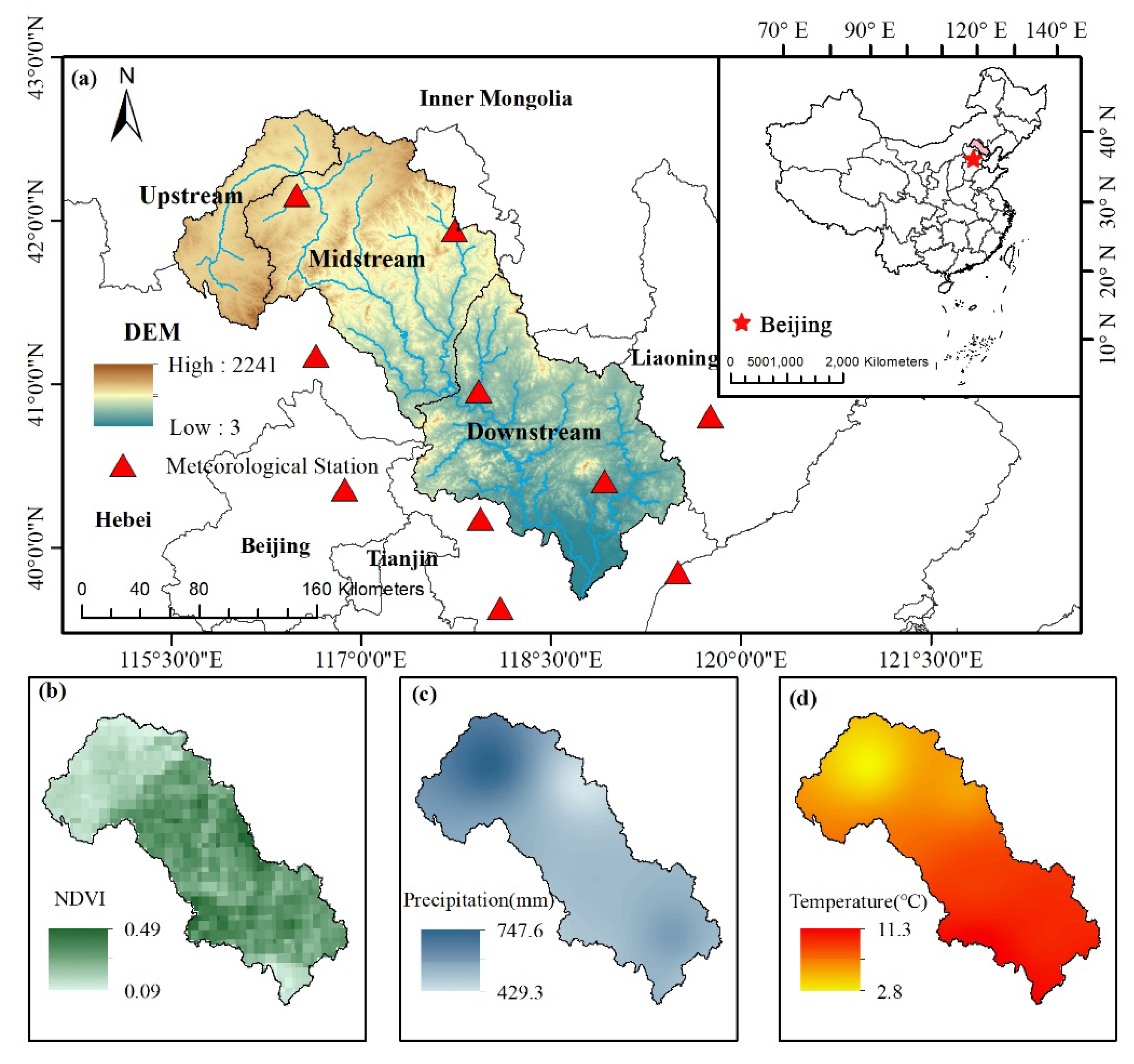
2.1. Study Area

The Luanhe River Basin (LRB), covering a total area of 44,793.51 km², as shown in Figure 1, was selected as the study catchment. The LRB is located northeast of Beijing, China (115°30′ E–119°45′ E, 39°10′ N–42°40′ N), and is characterized as an important ecological barrier to alleviate the effect of sandstorms from Mongolia and conserve water resources for the Beijing–Tianjin–Hebei region. The Luanhe River is not a tributary of the Hai River, but an independent river following the Hai River into the sea. The elevation ranges from 3 to 2241 m and decreases from the mountainous areas in the northwest to a plain in the southeast. The LRB is situated in a typical temperate continental monsoonal zone with semi-arid climate [17], where is more sensitive to climatic and anthropogenic disturbance. The study catchment has an annual temperature fluctuating from 0 °C to 9.0 °C and 478.5 mm of average annual precipitation. Heavy rainfall and relatively high temperature occur in summer, and less rainfall and low temperature occur in winter.

To provide more specific ecological conservation management strategies based on the characteristics of vegetation types in the study catchment, sub-watersheds with different landscapes should be considered. Therefore, three sub-watersheds were identified based on the landcover characters: Upstream (6405 km², 15.25% of the total area), midstream (18,394 km², 43.57% of the total area), and downstream (19,807 km², 41.18% of the total area) (Figure 1).

In particular, agricultural land in the upstream (31.33% in 1980 and 32.38% in 2015) had the greatest contribution among the sub-watersheds. As part of the ecological conservation area, the midstream and downstream were mostly covered by forest and herbaceous vegetation and did not change during 1980–2015. The forest covers about 45% and 44% at midstream and downstream, respectively, and the herbaceous covers about 29% in both these two sub-watersheds. The urban area was mainly situated in the downstream area, with 1.64% in 1980 and 2.27% in 2015 (Figure 2). These three sub-watersheds can be categorized by their typical land use types as agriculture area (upstream), forest conservation area (midstream), and forest–urban area (downstream).

2.2. Data Sets

2.2.1. Data Source

LULC (land use and land cover) maps with a 1000 m resolution was provided by the Resource and Environmental Data Cloud Platform of the Chinese Academy of Sciences (http://www.resdc.cn). The monthly climatic data from ten meteorological stations, including precipitation and temperature, from 1982 to 2015 was provided by the National Meteorological Administration of China (http://data.cma.cn). The monthly Normalized Difference Vegetation Index (NDVI) data (0.05 degree resolution) from 1982 to 2015 was obtained from the Advanced Very High Resolution Radiometer (AVHRR) of US National Oceanic and Atmospheric Administration (NOAA) (https://nex.nasa.gov) to quantify the variation of vegetative cover changes in the LRB.

In our research, the growth seasons include late spring (April to May), summer (June to August) and early autumn (September to October). The winter has been ignored, because of the low vegetation growth rate during chilly climate in the study catchment [18]. The average NDVI value during summer, early autumn and late spring was 0.611, 0.459, and 0.354, respectively. The NDVI for the three sub-watersheds from higher to lower is in the order of downstream, midstream and upstream, which is directly opposite to the elevational change. Moreover, most of the NDVI in the LRB from 1982 to 2015 has shown an increasing trend in different sub-watersheds during the growing seasons, except for the upstream during late spring (Figure 3). Meanwhile, the upstream also showed the smallest increasing tendency compared to that of the other sub-watersheds during all three seasons (Figure 3).

2.2.2. Data Pre-Treatment

In our study, we address the climate factors (precipitation and temperature) and the vegetation growth (NDVI) at monthly scale in the three sub-watersheds. To achieve this research goal, the data pre-treatment was procedure as follows: first, for the climate factors, we interpolate the monthly precipitation and temperature data from the meteorological stations and re-summarized the climate data as the average value for each sub-watershed; second, in order to match the format of climate data, the raster NDVI was also categorized as the average value at monthly scale and calculated into different sub-watershed using the GIS (zonal statistics tool).

3. Methods

A multi-statistical method is proposed in our study to characterize how vegetation changes in response to temperature and precipitation. As the flowchart shows in Figure 4, the procedure is as follows: (a) The collection and pre-treatment of vegetation and climatic data, (b) bivariate correlation assessment by the tail features based on the different fitted copulas, (c) using composite Granger causality test to detect both the causal relationship and legacy effect between NDVI-T/P, (d) take the different sub-watersheds and growth seasons into consideration, we address several implications for policymakers and stakeholders. The detailed instructions for the statistical methods are described in the “Methods” section of supplementary information.

3.1. Copula Based Bivariate Correlation Assessment

The most commonly used Copula functions, which were designed to assess bivariate joint dependence structures, have been divided into two families, elliptical (Gaussian and Student’s t-Copula) and Archimedean (Clayton, Gumbel, and Frank). Because elliptical Copulas are derived from the well-known distribution types and widely used Pearson’s correlation, the elliptical Copula has become popular in most fields. However, the elliptical is only able to reproduce an expression that is symmetrical [19]. The Archimedean Copulas (

Table 1. Equations for the Archimedean Copula functions, where u and v are defined as two marginal distribution and θ is the dependence parameter.

Family	C (u, v)	Parameter
Clayton	$({\mathrm{u}}^{-\theta }+v^{-\theta }-1{)}^{-1/\theta }$	$0\le \theta$
Frank	$-\frac{1}{\theta }\ln (1+\frac{(e^{-\theta u}-1)(e^{-\theta v}-1)}{e^{-\theta }-1})$	$\theta \ne 0$
Gumbel	$e^{{\left[{(-\ln u)}^{\theta }+{(-\ln v)}^{\theta }\right]}^{1/\theta }}$	$1\le \theta$

), including the Gumbel, Frank, and Clayton Copulas, have an explicit formula and are quite popular given their ability to capture a wider variety of joint dependence structures [20].

In our study, we use Akaike information criterion (AIC) and Root Mean Square Error (RMSE) to select best fitted Archimedean Copulas. The smaller the AIC and RMSE value, the better results for the Copula to interpret the correlation between vegetative growth and climatic factors. Moreover, we use diverse tail features of different Archimedean Copula to detect the bivariate correlation between NDVI and climatic factors (Figure 4). For each Archimedean Copula, the distribution shows unique features. If two variables can be described by the Clayton Copula, there is a strong correlation between the variables at the lower tail, while the variables are gradually independent at the upper tail. In contrast to the Clayton Copula, the Gumbel Copula shows a strong correlation between variables at the upper tail, while at the lower tail the variables are gradually independent. The Frank Copula has symmetrical tail characteristics, which means it cannot capture the asymmetrical tail characteristics between random variables. The correlation coefficient of the variables at the tail is zero, which indicates that the variables at both tails are gradually independent [19].

3.2. Composite Granger Causality Test for Legacy Effect and Casual Relationship

Originally, the stationary sequence has been required to operate the Granger causality test. To extend the Granger causality test to fit a more general data sequence, Engle–Granger cointegration test (EG test) has been regarded as an irreplaceable premise to broaden the scope of applicability in our study [21]. The Engle–Granger cointegration test can be used to prove two non-stationary data sequences may have stationary relation over long time period. In order to examine whether the data sequence has passed the EG test, the Durbin–Watson (DW) coefficient was introduced, when the DW approaches 2, the data sequence would be recognized to obey the normal distribution and can be recognized to have stationary relation. In addition, the vector autoregression (VAR) model [22] has been applied to investigate the legacy effect between NDVI and climatic factors, using the Akaike information criterion (AIC). Although the Granger causality test can be used on any lag length between these sequences, the significance of the Granger causality test is better based on the optimal lag length which was indicated by the minimum AIC.

The overall processes are listed in Figure 4: (1) The sequences have been first tested by the Augmented Dickey–Fuller Test (ADF) for stationarity, (2) the non-stationary sequence has to been further examined by Engle–Granger cointegration test, while the stationary sequence can be analyzed by the VAR model directly to disclose the legacy effect, and (3) the optimal leg length detected by the VAR model would be used to conduct the Granger causality test.

4. Results

4.1. Nonlinear Bivariate Correlation between NDVI and Precipitation/Temperature

When the most appropriate marginal distribution has been determined, the Root Mean Square Error (RMSE) and Akaike information criterion (AIC) were used as two criteria to quantify the deviation between these data sequences. The most appropriate Copulas from Archimedean family (including the Clayton, Frank, and Gumbel Copulas) was selected to identify the relationship between seasonal NDVI-P and NDVI-T. The results of Copula selection are listed in

Table 2. The Root-Mean-Square Error (RMSE) and Akaike Information Criterion (AIC) of Frank, Clayton, and Gumbel copulas.

Season	Sub-Watersheds	Series	Frank		Clayton		Gumbel
			RMSE	AIC	RMSE	AIC	RMSE	AIC
Late Spring	Upstream	NDVI-P	0.067	−4.403	0.068	−4.365	0.074	−4.219
		NDVI-T	0.024	−6.460	0.027	−6.253	0.056	−4.767
	Midstream	NDVI-P	0.108	−3.457	0.105	−3.498	0.119	−3.258
		NDVI-T	0.046	−5.168	0.045	−5.213	0.095	−3.705
	Downstream	NDVI-P	0.138	−2.966	0.133	−3.032	0.153	−2.751
		NDVI-T	0.059	−4.778	0.061	−4.604	0.118	−3.268
Summer	Upstream	NDVI-P	0.060	−4.633	0.063	−4.530	0.060	−4.629
		NDVI-T	0.055	−4.787	0.057	−4.733	0.060	−4.636
	Midstream	NDVI-P	0.039	−5.493	0.040	−5.449	0.040	−5.424
		NDVI-T	0.039	−5.502	0.043	−5.279	0.044	−5.246
	Downstream	NDVI-P	0.047	−5.108	0.048	−5.072	0.048	−5.086
		NDVI-T	0.049	−5.027	0.051	−4.952	0.052	−4.901
Early Autumn	Upstream	NDVI-P	0.087	−3.797	0.086	−3.885	0.091	−3.792
		NDVI-T	0.039	−5.465	0.039	−5.477	0.079	−4.068
	Midstream	NDVI-P	0.108	−3.454	0.111	−3.393	0.115	−3.329
		NDVI-T	0.051	−4.966	0.057	−4.712	0.106	−3.496
	Downstream	NDVI-P	0.095	−3.698	0.101	−3.575	0.106	−3.488
		NDVI-T	0.059	−4.667	0.064	−4.496	0.097	−3.662

Note: The bold letters represent the most appropriate RMSE and AIC for determining the Copulas.

. And the results of the premise process for identifying the marginal distribution has been mentioned in the supplementary Table S1.

Based on the AIC and RMSE values, the Clayton and Frank Copulas are the most appropriate Copulas in fitting the joint distribution of seasonal NDVI-P and NDVI-T. Particularly, the RMSE and AIC values of the Frank Copula in fitting the NDVI-T series during the late spring and summer are the lowest, indicating that NDVI-T can be well described by the Frank Copula during this period. Likewise, the Clayton Copula showed better agreement with the joint distribution of NDVI-T during early autumn in the upstream. Whereas, different from the homogeneity of the Copula for NDVI-T during late spring and summer, the Copulas varied by seasons and sub-watershed for NDVI-P. For NDVI-P, the Frank Copula was better to fit the joint distribution for all three sub-watersheds during the summer. In contract to the other sub-watersheds, the Frank and Clayton Copula was employed to describe the relationship between NDVI-P in upstream during the late spring and early autumn, respectively.

4.2. Granger Cause and Legacy Effect

4.2.1. Time Series Sequence Identification

The premise of the composite Granger causality test is that the data sequence needs to be stationary or have two data sequences that are of the same order to meet the requirement of a cointegration relationship [23]. If the vegetation and climatic data sequence passes the ADF test, then the sequence has been recognized as stationary. However, if the sequences do not pass the ADF test, then the Engle–Granger cointegration test is introduced to determine whether there is a cointegration relationship between the NDVI and precipitation/temperature. The time sequence identification results for the NDVI, precipitation and temperature are listed in

Table 3. Results of Augmented Dickey–Fuller Test (ADF) test for vegetation and climatic sequence.

Sub-Watersheds	Factors	ADF Coefficient	t-Statistic	p	Conclusion
Upstream	NDVI	−3.914	−3.421	0.012	Stationary
	T	−3.701	−3.422	0.023	Stationary
	P	−4.31	−3.421	0.003	Stationary
Midstream	NDVI	−2.727	−3.421	0.066	Non-stationary
	T	−3.791	−3.422	0.018	Stationary
	P	−4.434	−3.421	0.002	Stationary
Downstream	NDVI	−3.309	−3.421	0.046	Stationary
	T	−3.774	−3.421	0.018	Stationary
	P	−4.302	−3.421	0.003	Stationary

. The highlighted NDVI sequence in the midstream is non-stationary with a p-value greater than 0.05, while the other sequence for these three factors is stationary.

To identify whether the non-stationary sequence of the NDVI has a cointegration relationship with precipitation or temperature, the Engle–Granger cointegration test was conducted (Figure 5). The Durbin–Watson (DW) coefficient for NDVI-P and NDVI-T is 1.56 and 1.89, respectively. The specific statistical results are listed in supplementary Table S2. The criteria for whether there exists a cointegration relationship, depends on whether the DW coefficient is closer to 2 [24]. According to Figure 5, the NDVI-P has a relatively weak cointegration relationship in the midstream. Therefore, there would be no obvious causal relationship at the midstream between NDVI-P.

4.2.2. Optimal Lag Length and Granger Causality

After confirming the stationary and Engle–Granger cointegration relationship between the sequences of the variables, the Granger causality test can be used to discriminate the interactive relationship among the variables. In our study, the optimal lag length between the NDVI-T and NDVI-P was identified before the Granger causality test was carried out by the VAR model.

Notably, the minimum AIC value for detecting the optimal lag length varied between sub-watersheds for the NDVI-T/P (Figure 6). The optimal lag length of the NDVI-T between the upstream, midstream and downstream is 2, 4, and 4 months, respectively. Because the result for the precipitation either shows a stationary or cointegration relationship with NDVI in the midstream, the lag length for NDVI-P has only been identified in the upstream and downstream with 2 and 3 months, respectively.

The Granger causality test was conducted at the 95% confidence level. The null hypothesis for each NDVI-T/P in different sub-watershed is that “the climate factors/NDVI is not the Granger cause of the NDVI/climate factors”. When p-value is less than 0.05, the null hypothesis would be rejected. The results in

Table 4. The Granger causality test results for different sub-watersheds at the optimal lag length.

Sub-Watershed	Optimal Lag Length	H0 (Null Hypothesis)	F-Statistics	p-Value	Conclusion
Upstream	2	NDVI is not the Granger cause of Precipitation	3.078	0.1011	Accept
		Precipitation is not the Granger cause of NDVI	12.6634	0.0031	Reject
Downstream	3	NDVI is not the Granger cause of Precipitation	1.5953	0.2464	Accept
		Precipitation is not the Granger cause of NDVI	5.0371	0.028	Reject
Upstream	2	NDVI is not the Granger cause of Temperature	0.132	0.9383	Accept
		Temperature is not the Granger cause of NDVI	13.3876	0.0001	Reject
Midstream	4	NDVI is not the Granger cause of Temperature	0.8006	0.6574	Accept
		Temperature is not the Granger cause of NDVI	22.8862	0.0012	Reject
Downstream	4	NDVI is not the Granger cause of Temperature	0.9745	0.5788	Accept
		Temperature is not the Granger cause of NDVI	35.8145	0.0007	Reject

indicate that for all three sub-watersheds with stationary or modified climate and NDVI data sequences, the temperature/precipitation has been identified as the Granger cause of the NDVI.

5. Discussion

5.1. NDVI Response to Temperature

In most cases, the correlation between temperature and NDVI obeys the Frank Copula, which has no significant features for tail distribution. This consistency among different sub-watersheds and seasons suggests that temperature within the specific range in the study catchment has a direct effect on the vegetation growth rate [25]. The features showing no obvious upper or lower tail indicates that different from humid regions where a strictly positive relationship between the NDVI and temperature was found [26], the vegetation growth in a semi-arid area is not strictly positive along with the temperature, while a partially positive correlate relation has been noticed. The possibly reasons are listed below: first, due to the lack of rainfall, excessive warming may accelerate evaporation of soil water content and result in drought, which may lead to a negative effect on the biophysical process of plants.; second, given the excessive temperature, vegetation will prevent its own water loss by reducing leaf area and light saturation point, finally resulting in a decrease in vegetative cover [27]; third, an increase in temperature may promote autotrophic respiration and the transpiration rate, which may result in accelerating the consumption of organic matter and causing a decrease in the net productivity of vegetation [28]. Therefore, we conclude that vegetation growth in this semi-arid area present higher sensitivity to temperature than in humid areas.

Notably, different Copula patterns were found between the upstream (Clayton Copula) and midstream/downstream (Frank Copula) in early autumn. A larger and significant correlation coefficient was found at the upstream where the temperature and NDVI are both relatively low, which obey the Clayton Copula. This may result from the differences in land use type. The upstream region covers a large amount of cropland (>30%), where the NDVI has been largely reduced along with the temperature during early autumn by the agricultural activities, including harvesting and ploughing.

Furthermore, the two to four month lag length of NDVI in response to temperature for distinct sub-watersheds reveals that the vegetation may not have a synchronous response to temperature changes. As vegetation mainly accumulates nutrients and organic matter in spring and grows in summer and autumn [29], the distinct dominant and diversity of the vegetation types would be the main cause of different legacy effect for NDVI in response of the temperature. The agricultural area (upstream) presented a faster responce to temperature than the forest conservation area in the midstream and forest–urban mixed area in the downstream, which may be due to the short growth cycle and rapid growth rate of the crops [30]. The mature forest, protected by the national and local government, requires more energy to growth, which is produced from the photosynthetic processes [31] and finally result in the slowest response rate in the forest-dominant area (midstream and downstream).

5.2. NDVI Response to Precipitation

During late spring, the correlation between NDVI and precipitation in the upstream not only shows different fitting features (Frank Copula) to those of the midstream and downstream (Clayton Copula) but also has a short response time (2 months), which indicates that the crops are more sensitive to precipitation for growth in spring. When taking the longer lag length (3 months) for the NDVI in response to precipitation in the downstream into consideration, the forest and herbaceous in the forest–urban area (downstream) may retain a longer period for growth than the crops. These results imply that, in semi-arid area, the crops may have a better ability to take advantage of the restricted available water than forest to boost growth in spring [32]. However, the forest would present a longer time to accumulate nutrient in spring and exhibit stable growing rate during the whole growth season even in autumn [33].

In summer, the correlation between NDVI and precipitation was accumulated within a specific range, following the Frank Copula, in all three sub-watersheds. In contrast to previous studies in central Asia, which indicate a positive correlation between NDVI-P [34]. The fitted Frank Copula in the study catchment suggested that excessive rain in summer can suppress plant growth by limiting root respiration rates, and lead to the reduction on growth and coverage [35], in semi-arid area. Additionally, similar to NDVI-T, the harvest work could be the key reason for reducing the leaf cover and a lower tail relationship (Clayton Copula) between the NDVI and precipitation in the upstream, during the early autumn. Furthermore, the utilization of ground water resource in the upstream could accelerate the depletion of the available water for vegetation growth, especially in the autumn with less rainfall to replenish the ground water in semi-arid area [36]. The lack of a causal relation for the midstream sub-watershed, may due to the great amount of ground water conservation ability, which could help the vegetation to prevent drought or flood for a stable growth rate [30].

5.3. Implication

The multi-statistical methods, which expedite identification of the characteristics of the relationship between the NDVI and climatic factors (temperature and precipitation), can be used to aid in understanding the vegetation response to climate change, and thus be helpful for environmental management or investment decisions. To better fulfill the expectation of residents for the natural environment, national and local policy makers are anxious to find an effective way to balance economic development and ecosystem service provision [37]. However, as a result of rapid urbanization and population growth in China [38], it is difficult to establish a pure national park or conservation area without anthropogenic disturbance. Our mathematical work provides several potential clues for identifying a method for proposing cost-effective regulation, in order to better enhance or restore ecological conservation areas. According to the composite Granger causality test, temperature/precipitation has a considerable contribution to the vegetation compared to the impact of the vegetation on the regional temperature/precipitation. Therefore, the proposals for the conservation management are mainly based on the factors, which can be handled by humans to alleviate the negative impact of climate change on vegetation growth, such as the water supply and regulation criteria.

Our research suggests that, compared to the forest conservation and forest–urban mixed area, in the agricultural area in the upstream an important priority is to ensure the crops can acquire sufficient water in spring, especially when drought occurs. In addition, ground water resources play a critical role in vegetation growth, especially in the semi-arid area. Ground water conservation can well stimulate vegetation growth, when there is less rainfall. However, ground water deficits would largely affect agricultural efficiency [39]. Therefore, measures, such as utilization of groundwater and surface water for irrigation, as well as the development of a backup water source, should be regulated, in order to guarantee the growth of the crops. Different from forest and herbaceous, crops are more sensitive to water supply to promote growth, more water can motivate the dynamic processes in nutrient and mineral solution in the soil, which can be absorbed by vegetation under water-soluble conditions to yield more organic matter [40]. Then, physiological and biochemical processes such as photosynthesis and transpiration of crops can promote the growth rate [41]. Therefore, further researches and experiments regarding how to quantify the needed water for distinct plants should proceed for agricultural management in future.

Besides the climate factors, anthropogenic disturbance has been identified to be another key driver for vegetative growth [42]. It is acknowledged that over-grazing and over-cultivation were two major causes of reduced vegetative growth, especially in semi-arid areas, where the ecosystem is fragile [43]. Over-grazing would threaten vegetation species composition, variety and richness [44], while the over-cultivation may significantly deplete ground water for both human and crops [36]. In our study catchment, owing to the Grain for Green Program and environmental protection regulation since 1962, grazing and cultivation activities have been limited. In order to honor the great efforts for environmental protection, the LRB is internationally known for the Saihanba National Forest Park, who has won the award for Champions of the Earth in 2017 from the United Nations Environment Programme [45]. Some policymakers think that the ecological immigration, which aims at moving the local people to other regions would be a reliable measurement to regulate the nonnegligible anthropogenic disturbance in the National Park. However, the national and local policy makers and stakeholders can benefit from our findings to carry out more cost-effective regulations for better conserving the ecosystem services. Two indicators in our study have indicated that, for the policy makers, a more cost-efficient regulation to alleviate the negative effects of human activities in the conservation area or a national park would be to provide effective limitations to regulate human activities rather than migrate all residents outside of the conservation area. One indicator is that, as shown in Figure 2, the difference in the NDVI between the midstream and downstream is relatively narrow, which may be mainly due to the altitude gradient. With an increase in altitude, the temperature, atmospheric pressure and partial pressure of CO₂ would decrease [46], which result in the lower organic synthesis rate [31]. The other indicator is the consistency of the NDVI change trend, fitted Copula function and the same lag length identification between the midstream and downstream. These facts may be among the indicators that when appropriate regulation has been carried out, limited urbanization or anthropogenic disturbance would not have largely negative effects on the conservation area. Several researches have indicated that the limited and regulated urbanization processes, including low impact development, would strengthen the resistant ability for residential areas and reduce the negative impact on ecosystems [47]. Therefore, how to quantify and control the accepted human activities and urbanization should be further discussed.

To conclude, the multi-statistical methods proposed in this study provide a general measure to bridge the data gaps between stationary or non-stationary sequence and reject the pseudo regression. In addition, this method can be applied to not only identify the relationship between the NDVI and climatic factors but also detect the legacy effect and causal relationship. Our methods would be suitable for both researchers and policymakers with different intentions. For policy makers, our study implies that (1) the agriculture area should be ensured to have plenty of water prior than the forest-dominant area; and (2) the restricted regulation to limit human activities would be more cost-effective to protect the forest ecosystem in study catchment. For researchers, our research could be meaningful in following aspects: (1) The multi-statistical methods may improve the understanding of the relationship between two sequences, (2) the further studies on water demand for specific crops would help policy makers to carry out appropriate irrigation measures; and (3) how to quantify the accepted human activity in forest–urban mixed area would help local residents to achieve sustainable goals.

5.4. Limitation and Uncertainty

In our study, temperature and precipitation data have been analyzed as independent variables to affect the vegetation growth. However, in the natural ecological system, the temperature and precipitation-related climatic variables generally interact and determine plant growth. The independent indicator using in our study may therefor generate uncertainty regarding influences of precipitation and temperature on vegetation growth. Therefore, the interactive indices, such as combination of effect of relative air humidity, soil water content, evaporation rate, and (bio)climatic index, merit further studies, especially experimental studies, for vegetation growth.

6. Conclusions

This study provides a multi-statistical assessment method to address the characteristics of the NDVI and climatic factors (temperature and precipitation). This methodology transferring from economics to the environmental sciences field is promising and provides a comprehensive and simpler applicable approach to indicate a basis for evaluating the relationship and casualty between vegetative growth and climatic factors. The conclusions of this study are as follows:

(1) Except for the NDVI-P in the midstream, which has no presented obvious causality relationship, both temperature and precipitation were identified as the Granger causes for the NDVI changes in most of the study area.

(2) The NDVI in semi-arid area is different with the other climatic zone that is not strictly positive to temperature and precipitation change. The excessive warmth and precipitation would inhibit the vegetative growth during the growing seasons.

(3) Crops show the two months lag length in response to temperature, while other forest-dominated area has presented four months lag in response to the temperature. Thus, crops respond to temperature faster than forest and herbaceous at the semi-arid area.

(4) Based on the NDVI change characteristics and assessment using these two statistical methods, we found that limited human activities in the ecological conservation area would not result in major negative effects on vegetative growth.

References

1. Scheiter, S.; Higgins, S.I. Impacts of climate change on the vegetation of Africa: An adaptive dynamic vegetation modelling approach. Glob. Chang. Biol. 2009, 15, 2224–2246. [Google Scholar] [CrossRef]
2. Hou, G.; Zhang, H.; Wang, Y. Vegetation dynamics and its relationship with climatic factors in the Changbai Mountain Natural Reserve. J. Mt. Sci. 2011, 8, 865–875. [Google Scholar] [CrossRef]
3. Xu, H.-J.; Wang, X.-P.; Yang, T.-B. Trend shifts in satellite-derived vegetation growth in Central Eurasia, 1982–2013. Sci. Total Environ. 2017, 579, 1658–1674. [Google Scholar] [CrossRef] [PubMed]
4. Geng, X.; Zhou, X.; Yin, G.; Hao, F.; Zhang, X.; Hao, Z.; Singh, V.P.; Fu, Y.H. Extended growing season reduced river runoff in Luanhe River basin. J. Hydrol. 2020, 124538. [Google Scholar] [CrossRef]
5. Fu, Y.H.; Piao, S.; Zhao, H.; Jeong, S.-J.; Wang, X.; Vitasse, Y.; Ciais, P.; Janssens, I.A. Unexpected role of winter precipitation in determining heat requirement for spring vegetation green-up at northern middle and high latitudes. Glob. Chang. Biol. 2014, 20, 3743–3755. [Google Scholar] [CrossRef] [PubMed]
6. Piao, S.; Mohammat, A.; Fang, J.; Cai, Q.; Feng, J. NDVI-based increase in growth of temperate grasslands and its responses to climate changes in China. Glob. Environ. Chang. 2006, 16, 340–348. [Google Scholar] [CrossRef]
7. Piao, S.; Wang, X.; Ciais, P.; Zhu, B.; Wang, T.A.O.; Liu, J.I.E. Changes in satellite-derived vegetation growth trend in temperate and boreal Eurasia from 1982 to 2006. Glob. Chang. Biol. 2011, 17, 3228–3239. [Google Scholar] [CrossRef]
8. Chu, H.; Venevsky, S.; Wu, C.; Wang, M. NDVI-based vegetation dynamics and its response to climate changes at Amur-Heilongjiang River Basin from 1982 to 2015. Sci. Total Environ. 2019, 650, 2051–2062. [Google Scholar] [CrossRef]
9. Lamchin, M.; Lee, W.-K.; Jeon, S.W.; Wang, S.W.; Lim, C.H.; Song, C.; Sung, M. Long-term trend and correlation between vegetation greenness and climate variables in Asia based on satellite data. Sci. Total Environ. 2018, 618, 1089–1095. [Google Scholar] [CrossRef]
10. Igbawua, T.; Zhang, J.; Chang, Q.; Yao, F. Vegetation dynamics in relation with climate over Nigeria from 1982 to 2011. Environ. Earth Sci 2016, 75, 596. [Google Scholar] [CrossRef]
11. Al-Harthy, M.; Begg, S.; Bratvold, R.B. Copulas: A new technique to model dependence in petroleum decision making. J. Pet. Sci. Eng. 2007, 57, 195–208. [Google Scholar] [CrossRef]
12. Kendall, M.G. A new measure of rank correlation. Biometrika 1938, 30, 81–93. [Google Scholar] [CrossRef]
13. Sklar, M. Fonctions de repartition a n dimensions et leurs marges. Publ. Inst. Stat. Univ. Paris 1959, 8, 229–231. [Google Scholar]
14. Kong, D.; Miao, C.; Duan, Q.; Lei, X.; Li, H. Vegetation-Climate Interactions on the Loess Plateau: A Nonlinear Granger Causality Analysis. J. Geophys. Res. 2018, 123, 11068–11079. [Google Scholar] [CrossRef]
15. Granger, C.W.J. Investigating Causal Relations by Econometric Models and Cross-spectral Methods. Econometrica 1969, 37, 424. [Google Scholar] [CrossRef]
16. Granger, C.W.J.; Siklos, P.L. Systematic sampling, temporal aggregation, seasonal adjustment, and cointegration theory and evidence. J. Econom. 1995, 66, 357–369. [Google Scholar] [CrossRef]
17. Zhang, X.; Xu, Y.; Hao, F.; Li, C.; Wang, X. Hydrological Components Variability under the Impact of Climate Change in a Semi-Arid River Basin. Water 2019, 11, 1122. [Google Scholar] [CrossRef] [Green Version]
18. Weiser, C.J. Cold Resistance and Injury in Woody Plants: Knowledge of hardy plant adaptations to freezing stress may help us to reduce winter damage. Science 1970, 169, 1269–1278. [Google Scholar] [CrossRef]
19. Nelsen, R.B. An introduction to Copulas, 2nd. ed.; Corr. 2. pr. Softcover version of original hardcover edition 2006; Springer: New York, NY, USA, 2010; ISBN 9780387286785. [Google Scholar]
20. Ribeiro, A.F.S.; Russo, A.; Gouveia, C.M.; Páscoa, P. Copula-based agricultural drought risk of rainfed cropping systems. Agric. Water Manag. 2019, 223, 105689. [Google Scholar] [CrossRef]
21. Tu, C. Cointegration-based financial networks study in Chinese stock market. Phys. A Stat. Mech. Its Appl. 2014, 402, 245–254. [Google Scholar] [CrossRef]
22. Sims, C.A. Macroeconomics and Reality. Econometrica 1980, 48, 1. [Google Scholar] [CrossRef] [Green Version]
23. Maziarz, M. A review of the Granger-causality fallacy. J. Philosoph. Econ. Reflect. Econ. Soc. Issues 2015, VIII, 86–105. [Google Scholar]
24. Nerlove, M.; Wallis, K.F. Use of the Durbin-Watson Statistic in Inappropriate Situations. Econometrica 1966, 34, 235. [Google Scholar] [CrossRef]
25. Lucht, W.; Prentice, I.C.; Myneni, R.B.; Sitch, S.; Friedlingstein, P.; Cramer, W.; Bousquet, P.; Buermann, W.; Smith, B. Climatic control of the high-latitude vegetation greening trend and Pinatubo effect. Science 2002, 296, 1687–1689. [Google Scholar] [CrossRef] [PubMed] [Green Version]
26. Cui, Y. Preliminary Estimation of the Realistic Optimum Temperature for Vegetation Growth in China. Environ. Manag. 2013, 52, 151–162. [Google Scholar] [CrossRef] [PubMed]
27. Zhang, K.; Kimball, J.S.; Nemani, R.R.; Running, S.W.; Hong, Y.; Gourley, J.J.; Yu, Z. Vegetation Greening and Climate Change Promote Multidecadal Rises of Global Land Evapotranspiration. Sci. Rep. 2015, 5, 15956. [Google Scholar] [CrossRef]
28. Saxe, H.; Cannell, M.G.R.; Johnsen, Ø.; Ryan, M.G.; Vourlitis, G. Tree and forest functioning in response to global warming. New Phytol. 2001, 149, 369–399. [Google Scholar] [CrossRef]
29. Qian, Y.Q.; He, F.P.; Wang, W. Seasonality, rather than Nutrient Addition or Vegetation Types, Influenced Short-Term Temperature Sensitivity of Soil Organic Carbon Decomposition. PLoS ONE 2016, 11, e0153415. [Google Scholar] [CrossRef]
30. Monteith, J.L. The Photosynthesis and Transpiration of Crops. Exp. Agric. 1966, 2, 1–14. [Google Scholar] [CrossRef]
31. Criddle, R.S.; Hopkin, M.S.; Mcarthur, E.D.; Hansen, L.D. Plant distribution and the temperature coefficient of metabolism. Plant. Cell Environ. 1994, 17, 233–243. [Google Scholar] [CrossRef]
32. Ong, C.K.; Wilson, J.; Deans, J.D.; Mulayta, J.; Raussen, T.; Wajja-Musukwe, N. Tree–crop interactions: Manipulation of water use and root function. Agric. Water Manag. 2002, 53, 171–186. [Google Scholar] [CrossRef]
33. Mitchell, C.P.; Ford-Robertson, J.B.; Hinckley, T.; Sennerby-Forsse, L. Ecophysiology of Short Rotation Forest Crops; Springer: Amsterdam, The Netherlands, 1992; p. 8489. [Google Scholar]
34. Ichii, K.; Kawabata, A.; Yamaguchi, Y. Global correlation analysis for NDVI and climatic variables and NDVI trends: 1982–1990. Int. J. Remote Sens. 2002, 23, 3873–3878. [Google Scholar] [CrossRef]
35. Ukkola, A.M.; Prentice, I.C.; Keenan, T.F.; Van Dijk, A.I.; Viney, N.R.; Myneni, R.B.; Bi, J. Reduced streamflow in water-stressed climates consistent with CO2 effects on vegetation. nclimate 2016, 6, 75–78. [Google Scholar] [CrossRef] [Green Version]
36. Massoud, E.; Turmon, M.; Reager, J.; Hobbs, J.; Liu, Z.; David, C.H. Cascading Dynamics of the Hydrologic Cycle in California Explored through Observations and Model Simulations. Geosciences 2020, 10, 71. [Google Scholar] [CrossRef] [Green Version]
37. Bai, Y.; Ochuodho, T.O.; Yang, J. Impact of land use and climate change on water-related ecosystem services in Kentucky, USA. Ecol. Indic. 2019, 102, 51–64. [Google Scholar] [CrossRef]
38. Yang, X.J. China’s rapid urbanization. Science 2013, 342, 310. [Google Scholar] [CrossRef] [PubMed]
39. Massoud, E.C.; Purdy, A.J.; Miro, M.E.; Famiglietti, J.S. Projecting groundwater storage changes in California’s Central Valley. Sci. Rep. 2018, 8, 12917. [Google Scholar] [CrossRef] [PubMed]
40. Gourdji, S.M.; Sibley, A.M.; Lobell, D.B. Global crop exposure to critical high temperatures in the reproductive period: Historical trends and future projections. Environ. Res. Lett. 2013, 8, 24041. [Google Scholar] [CrossRef]
41. Victor, D.G.; Ausubel, J.H. Restoring the Forests. Foreign Aff. 2000, 79, 127. [Google Scholar] [CrossRef]
42. Zhang, P.; Cai, Y.; Yang, W.; Yi, Y.; Yang, Z.; Fu, Q. Contributions of climatic and anthropogenic drivers to vegetation dynamics indicated by NDVI in a large dam-reservoir-river system. J. Clean. Prod. 2020, 256, 120477. [Google Scholar] [CrossRef]
43. Qu, S.; Wang, L.; Lin, A.; Yu, D.; Yuan, M. Distinguishing the impacts of climate change and anthropogenic factors on vegetation dynamics in the Yangtze River Basin, China. Ecol. Indic. 2020, 108, 105724. [Google Scholar] [CrossRef]
44. Bakhshi, J.; Javadi, S.A.; Tavili, A.; Arzani, H. Study on the effects of different levels of grazing and exclosure on vegetation and soil properties in semi-arid rangelands of Iran. Acta Ecol. Sin. 2019. [Google Scholar] [CrossRef]
45. Zhao, P.; Fan, W.; Liu, Y.; Xu, X. Calculation of FAPAR over ragged terrains: A case study at Saihanba. In Proceedings of the 2016 IEEE International Geoscience & Remote Sensing Symposium, Beijing, China, 10–15 July 2016; pp. 3656–3659. [Google Scholar]
46. Loehle, C. Height growth rate tradeoffs determine northern and southern range limits for trees. J. Biogeogr. 1998, 25, 735–742. [Google Scholar] [CrossRef]
47. Steiner, K.; Herweg, K.; Dumanski, J. Practical and cost-effective indicators and procedures for monitoring the impacts of rural development projects on land quality and sustainable land management. Agric. Ecosyst. Environ. 2000, 81, 147–154. [Google Scholar] [CrossRef]
Figure 1. Location and the environmental condition of the Luanhe River Basin: (a) Location of the Luanhe River Basin; average (b) Normalized Difference Vegetation Index (NDVI) value, (c) precipitation and (d) temperature between 1982–2015.
Forests 11 00340 g001
Figure 2. Land use changes from 1980 to 2015 for the different sub-watersheds
Forests 11 00340 g002
Figure 3. NDVI change in sub-watersheds during different seasons, i.e., (a) late spring; (b) summer and (c) early autumn.
Forests 11 00340 g003
Figure 4. The schematic of the multi-statistical flowchart for vegetation in response to temperature and precipitation ((1) and (2) are the two components for multi-statistical method).
Forests 11 00340 g004
Figure 5. Results of the Engle–Granger cointegration test for the non-stationary sequence between NDVI-P (a) and NDVI-T (b) in the midstream.
Forests 11 00340 g005
Figure 6. Lag length of NDVI-T and NDVI-P in the three sub-watersheds
Forests 11 00340 g006