Article

Simulating Araucaria angustifolia (Bertol.) Kuntze Timber Stocks With Liocourt’s Law in a Natural Forest in Southern Brazil

by
Emanuel Arnoni Costa
1,2,*,
Veraldo Liesenberg
1,
André Felipe Hess
1,
César Augusto Guimarães Finger
3,4,
Paulo Renato Schneider
3,
Régis Villanova Longhi
5,
Cristine Tagliapietra Schons
3 and
Geedre Adriano Borsoi
1
1
Graduate Program in Forest Engineering, Santa Catarina State University (UDESC), Lages, Santa Catarina 88520-000, Brazil
2
Department of Forest Engineering, Federal University of Uberlândia (UFU), Monte Carmelo, Minas Gerais 38500-000, Brazil
3
Graduate Program in Forest Engineering, Federal University of Santa Maria (UFSM), Santa Maria, Rio Grande do Sul 97105-900, Brazil
4
Graduate Program in Agroecosystems, Federal University of Technology of Paraná (UTFPR), Dois Vizinhos, Paraná 85660-000, Brazil
5
Department of Forest Sciences, Federal University of Alagoas (UFAL), Maceió, Alagoas 57072-900, Brazil
*
Author to whom correspondence should be addressed.
Forests 2020, 11(3), 339; https://doi.org/10.3390/f11030339
Submission received: 28 January 2020 / Revised: 13 March 2020 / Accepted: 15 March 2020 / Published: 18 March 2020
(This article belongs to the Special Issue Climate Change Effect on Mixed-Species Forest Management)

Abstract

:
This paper presents a simulation of the regulation of Araucaria angustifolia (Bertol.) Kuntze timber stocks using Liocourt’s law. Although this species is currently protected by law, recent government initiatives are being considered to propose sustainable forest management practices by selecting small rural properties in Southern Brazil. Here, we simulate the applicability of Liocourt’s law in a typical rural property, the size of which is approximately 85 ha. Forest inventory measurements were conducted by estimating the diameter at the breast height (d), total height (h), and annual diameter increments of 308 trees that fit the criteria of d ≥ 10 cm, distributed on 35 permanent plots of 400 m2 each. As a result, a reverse J-shaped d distribution was found. On average, 303 trees can be found per hectare (ha). Local allometric equations showed their basal area (G) to be 21.9 m2∙ha−1, and their commercial volume (V) to be 172 m3∙ha−1, whereas Liocourt’s quotient (q) was 1.31. Based on these attributes, nine different forest management scenarios were proposed by simulating a remaining basal area (Grem) of 10.0, 14.0, and 18.0 m2∙ha−1, and Liocourt’s quotient was changed to 1.1, 1.3, and 1.5. All scenarios consider a d of 62.5 cm. In the less intensive scenario (i.e., q value = 1.5 and larger basal area of 18.0 m2·ha−1) there is greater optimization of space, and higher economic return is ensured to rural producers due to the definition of shorter cutting cycles. This also allows a faster growth rate in both d and h for smaller trees, due to the higher incidence of light onto the lower canopy layer, increasing the natural regeneration implementation of other native species. Forest management should thus be considered a goal in addition to consumer market characteristics for defining the ideal timber stock scenario.

1. Introduction

Mixed-species stands provide greater ecological and socio-economical services since they can be more resistant to natural disturbances [1,2], more stable with regard to climate change or disease control [3], and more productive than homogeneous stands [4,5]. Despite this, quantitative silvicultural guidelines facilitating the efficient management of mixed-species stands are still largely based on research information pertaining to pure even-aged stands [6].
Appropriate forest management practices serve to ensure that raw materials are exploited in a continuous and sustainable manner [7], i.e., by combining economic, social, and environmental benefits through efficient planning to allow the better management of the available resources, as exploiting more than the forest can produce at a given period may lead to the exhaustion of said resources, and removing less than what it can produce may lead to their underutilization and overpopulation, resulting in stagnation [8].
Growth and production models are important forest management planning tools, as they allow simulating the development of settlements and production under several management alternatives [9]. Cutting a single tree or a small group of trees distributed on a limited area creates spaces that can improve light conditions in the understory, promoting the growth of seedlings and young trees and improving the composition and structural diversity of plant species by forming habitats where they can coexist [10,11].
The regeneration and establishment of seedlings and their subsequent transition to larger classes must occupy the spaces left by the removal of bigger trees, with adequate intervals and intensity of cutting, which depend on the species’ regeneration and growth rates [12]. Given this context, it is important to obtain information that allows the rational management of one of the Atlantic Forest Biome’s most characteristic formations, found in the southern region of Brazil: Mixed Ombrophilous Forests (MOF) [13], also known as Araucaria Forests [14,15], with the implementation of plans and practices directed towards the species’ characteristics.
MOF are characterized by the presence of Araucaria angustifolia (Bertol.) Kuntze (referred to here as A. angustifolia), as it forms the upper canopy layer and has a dominant character in this vegetation type. In spite of this, the middle and lower layers demonstrate large diversities of species, such as Ocotea porosa (Nees & Mart.) Barroso, Luehea divaricata Mart., Cedrela fissilis Vell., Dicksonia sellowiana, and Maytenus ilicifolia Mart. ex Reissek [16,17]. As A. angustifolia is currently considered an endangered species and protected by law [18], the management of forested areas is mostly forbidden. However, recent government initiatives are being considered to show that natural forests in Southern Brazil can be sustainable and provide environmental, social and economic benefits besides being an important part of the life of local farmers [19,20].
Some studies have already verified the potential of regulating the diameter at the breast height (d) of A. angustifolia using Liocourt’ law [21] and quotient [22,23,24] to achieve sustainability by maximizing the growth of individual trees and, consequently, the production of timber [22,23,24]. However, all these studies fail to simulate changes of this quotient in association with the remaining basal area, which implies differences in cutting cycles and logging intensities. Such aspects must be clearly stated in sustainable forest management protocols by implementing reduced impact logging. More details and a better explanation of Liocourt’s law and its practical applications are available in Kerr [25], Gove [26], and Govedar et al. [27]. Therefore, this study sought to simulate the regulation of A. angustifolia timber stocks using Liocourt’s law in a typical rural property in the Southern region of Brazil. More specifically, it aimed to: (i) evaluate the forest’s current diametric structure; (ii) define different forest management scenarios for the species based on Liocourt’s law; (iii) evaluate the classification of wood assortment; (iv) provide insights for future forest management practices. We argue that sustainable forest management is the best way to promote the conservation of MOF and the renewal of this endangered species.
The remainder of this paper is organized as follows: Section 2 describes the rural property where this experiment was conducted and introduces the fundamentals of Liocourt’s law. The protocol followed in our experimental analysis is then presented. Section 3 shows the outcomes of the experiment and the simulation’s results, whereas Section 4 discusses the experimental results. Finally, Section 5 summarizes the main conclusions of this study, and points to future directions.

2. Materials and Methods

2.1. Study Site

The study site is located in a typical rural property in Southern Brazil, of the size of which is 83.5 hectares. It is located in the municipality of Lages (Santa Catarina, Brazil), and its central geographic coordinates are 27°48’ S and 50°19’ W. More than 50 ha of the rural property’s total size are covered by uneven-aged MOF, in which A. angustifolia is the dominant species. Although some authors consider A. angustifolia a pioneer species [28], there is also strong evidence that this is a climax species, which regenerates at different levels of light within the forest [29] and has seedlings that are extremely shade-tolerant [30]. The study site’s climate characterization, according to the Köppen classification, is mesothermic humid (Cfb), without dry season and with temperate summers. The areas’s altitude above sea level is approximately 987 m, with average annual temperature of 15.2 °C, and average annual precipitation of 1685.7 mm [31]. The predominant soil type in the region is Haplic Nitisol and Humic Cambisol, developed from basaltic rocks.

2.2. Data Collection and Preparation

A total of 35 permanent rectangular plots of 400 m2 each were installed in the study site using the fixed area method, and distributed using a systematic sampling approach. The spacing between sample plots was 50 m by 100 m, resulting in a grid. In each sample plot, all trees with diameter at breast height (d) equal to or greater than 10 cm were measured. Sample intensity and sampling error were evaluated according to the methodology proposed by Sanqueta et al. [32].
In addition, two perpendicular increment cores were radially extracted at d from the 308 measured trees using a Pressler borer. The sampling included trees in all d classes, covering the entire diametric amplitude of the species. Such measurements allow quantifying the periodical increment in d. The increment core samples were fixed to supports, air dried and sanded in a laboratory in order to make it easier to visualize the tree rings. Following the delimitation of the tree rings, the samples were digitally scanned (1200 pixels resolution). After scanning, the last five tree rings (corresponding to the last five years of growth) were measured using Image Pro-Plus© (Media Cybernetics Inc., Silver Spring, MD, USA).

2.3. Data Analysis

2.3.1. Balanced Frequency Distribution

After field data collection, the individuals were divided into diametric classes with regular 5-cm intervals to evaluate the forest’s diametric structure. Meyer’s equation [33,34] was adjusted to the sample units’ data to represent the estimated frequency distribution per unit area as seen in Equation (1):
Ni = β 0 · e β 1 · d i · ε
where: Ni = frequency per hectare in diametric class i; di = d class center, in cm; β0; β1 = estimated regression coefficients; e = base of natural logarithm; ε = residual error.
The balanced frequency distribution was then applied according to Liocourt’s law, demonstrating the proportionality between the number of trees of the current class and the subsequent one; this reason is called Liocourt’s quotient, or “q” [35]. Based on the angular coefficient (β1) of Equation (1) adjusted to araucaria trees, it was possible to determine Liocourt’s quotient:
q = e   β 1   ( d i d i + 1 )
where: q = Liocourt’s quotient; di = class center of the current d in cm; di+1 = class center of the subsequent d, in cm; β1 = estimated regression coefficient.
Nine forest management scenarios were then simulated for a remaining basal area of 10.0, 14.0, and 18.0 m2·ha−1, changing Liocourt’s quotient to 1.1, 1.3, and 1.5, respectively. All scenarios consider a maximum desired d of 62.5 cm. Each scenario allows evaluating different management interventions and their possible implications under a rational and sustainable forest management.

2.3.2. Volume, Volume Increments, and Cutting Rate

For the volume calculation, we followed the Kozak model [36] (Equation (3)), adjusted to the same area of the study by Costa et al. [37]. The model showed adjusted determination coefficient (R2 adj.) = 0.980 and precision expressed by root mean square error in percentage (RMSE%) = 6.8.
d i = β 0   d β 1   β 2 d ( 1 h i / h 1 p ) β 3   ( h i h ) 2 + β 4   ln ( h i h + 0.001 ) + β 5   h i h + β 6   e ( h i h ) + β 7   ( d h   ) + ε
where: di = diameter in relative positions along the shaft in cm; h = total height in m; hi = relative height in m; d = diameter at breast height in cm; β0 = 0.8944; β1 = 1.0361; β2 = 0.9994; β3 = 0.0 (ns); β4 = −0.1885; β5 = 1.1267; β6 = −0.2960; β7 = −0.0420; (ns) = non-significant estimated regression coefficient at α = 5%, therefore, the model was adjusted without the respective coefficient; ε = residual error; ln = natural logarithm; p = inflection point considered in 1.3/h.
However, because it is not analytically integrable, the Kozak model required the use of numerical integration techniques to obtain the partial volume (vi) and total volume up to the crown (vtci). In this way, with the reconstitution of the radial increment data at d of the last five years, the volume at the beginning and end of the selected period was obtained using the numerical integral approach. In order to accomplish this, a set of scripts were created in Visual Basic using Simpson’s 1/3 rule method [38]. Then, the annual percentage of volume increments up to the crown (PAI%vtci) for each tree was obtained by Equation (4), and later adjusted by Equation (5) to describe the variation of volumetric increments in all the diametric distribution of the forest.
PAI % vtci   = [ ( vtci i + 5 vtci i ) / vtci i ] · ( 100 n )
where: PAI%vtci = annual percentage of volume increments up to the crown, with bark; vtcii+5 = total volume increments up to the crown at the end of the period in m3, with bark; vtcii = total volume increments up to the crown at the beginning of the period in m3, with bark; n = time period considered, in this case, five years.
ln   ( PAI % vtci ) = β 0 + β 1   ln   ( d ) + ε
where: PAI%vtci = annual percentage of volume increments up to the crown, with bark; d = diameter at breast height in cm; β0; β1 = estimated regression coefficients; ε = residual error.
Following the adjustment of Equation (5), the average cutting rate was determined (PAIM%vtci) by weighting the increment for the di class center, based on the volumes observed in the di classes, according to Equation (6) [22]:
PAIM % vtci = Σ   Vt i · PAI % vtci i / Σ   V i
where: PAIM%vtci = mean annual percentage of volume increments up to the crown, with bark; Vti = total volume increments up to the crown in the di class in m3·ha−1, with bark; PAI%vtcii = annual percentage of volume increments up to the crown in the di class.

2.3.3. Cutting Cycle

The cutting cycle was estimated using Equation (7), which assumes that the volumetric annual growth of a tree or settlement accumulates according to the compound interest law [7]:
Vt = Vr   ( 1 + i ) c c
where: Vt = total volume at the end of the period in m3·ha−1, with bark; Vr = remaining volume at the beginning of the period in m3·ha−1, with bark; i = annual growth rate; cc = cutting cycle in years.

2.3.4. Wood Assortments

Although the assortments may be redefined to any dimension with the use of Equation (3), for this simulation, the assortments with bark were divided into four scenarios, as follows: S1 = timber destined for sawmills with d ≥ 40 cm and length of 5.4 m; S2 = timber destined for sawmills with d ≥ 30 cm and ≤40 cm, and length of 2.7 m; S3 = timber destined for sawmills with d ≥ 20 cm and ≤30 cm, and length of 2.2 m; S4 = timber destined for the energy or wood industry with d ≤ 20 cm and the remaining available length.
While defining the assortments, the formation of timber stocks with larger diameter and length was prioritized, following the sequence S1, S2, S3, and S4.

2.3.5. Statistical Analysis

All the statistical analyses were processed using the Statistical Analysis System [39]. In the evaluation of the generated models, we considered as goodness of fit criteria the coefficient of determination (R2) (Equation (8)) and the root mean square error (RMSE) (Equation (9)), in addition to the graphical analysis of the residuals.
R 2 = 1 [ i = 1 n ( y i y ^ i ) 2 i = 1 n ( y i y ¯ ) 2 ]
RMSE = i = 1 n ( y i y ^ i ) 2 n p
where: y i = observed values; y ¯ = average of the observed values; y ^ i = estimated values; n = number of observations; p = number of parameters.

3. Results

3.1. Diametric Structure of the Forest

Our selected forest showed a reverse J-shaped diameter distribution, characterized by lower entry rate and by the presence of individuals in the smaller diametric classes (i.e., between 30 and 50 cm in diameter). The relative sampling error was 11.6% for the mean value of the volume, indicating that, in the sampling design adopted, the error was usually close to what was proposed in common forest management projects (Ear ≤ 10.0%) [40]. Thus, the characteristics of the population were inferred at this precision level.
The frequencies observed according to diametric classes (Figure 1) indicate an unbalanced distribution. The observed basal area was 21.9 m2·ha−1, and the balanced frequency distribution for the entire rural property was predicted using Meyer’s relation (Equation (1)), with the value of Liocourt’s quotient (q) corresponding to 1.31. As a result, high adjustment and low error values can be noted.

3.2. Forest Management Scenarios Based on Liocourt’s Law

Figure 1 shows nine possible forest management scenarios by changing Liocourt’s quotient (q = 1.1, 1.3, 1.5) and setting the remaining basal area to 10.0, 14.0, and 18.0 m2∙ha−1. These scenarios were defined based on the forest’s current “q” value (1.31), simulating its maintenance (1.3), increase (1.5), or decrease (1.1), which is directly related to the number of individuals in the diametric classes. As a result, when the “q” value increases, the number of smaller trees in the forest also increases, whereas the number of larger trees decreases. Regarding the remaining basal area, the chosen values allowed the simulation of light (18.0 m2∙ha−1), moderate (14.0 m2∙ha−1), and strong (10.0 m2∙ha−1) silvicultural intervention. The latter, when the current basal area (21.9 m2∙ha−1) is reduced approximately by half, increases the number of candidate trees to be harvested in each diametric class. In summary, all these scenarios suggest possibilities of intervention in the forest while maintaining the balance of the current diametric structure.
The annual percentage of volume increments up to the crown, with bark (PAI%vtci), is presented in Figure 2a. It was determined according to the diametric classes, using (Equation (5)). The regression coefficients were quite significant, with R2 = 0.4475 and RMSE = 0.5764. Figure 2b shows the graphical residual analysis as a function of the estimated values. In general, they showed a regular distribution, without the presence of bias in the predictions. Despite the low R2 value, the model still explains almost 50% of the variation in the periodic increase in volume as a function of d. In this experiment, this value is not higher due to the lack of constancy in the increase in the growth rate of d in the last five years. However, this is a clear indication of the importance of forest management aimed at the conservation of this species.
The mean volume per hectare found in the forest was 172.0 m3∙ha−1, and the mean annual percentage of volume increments up to the crown (PAIM%vtci) was 2.44%. Based on these values, it was possible to simulate different management scenarios (Table 1).
The values of Table 1 vary according to the values of “q” and Grem considered. When considering q = 1.1 and Grem = 10.0 m2∙ha−1, the simulation shows that a volume of 82.7 m3∙ha−1 can be obtained every 27.2 years. By changing only the remaining Grem to 18.0 m2∙ha−1, it is possible to obtain a volume of 11.3 m3∙ha−1 every 2.8 years. Thus, the optimal scenario for intervention may vary according to the forest management goals.
It is important to mention that this specific species is not explored commercially since the 90s due to the restrictive legislation [19]. Recently, there are efforts being made to approve an ongoing project for A. angustifolia in the state of Santa Catarina, to regulate the planting, preservation, sustainable management, and development of silviculture and its proven food resources [41].
It was observed that a larger volume per hectare (observed V·ha−1) is found between classes with d ranging from 22.5 to 57.5 cm (Figure 3a). Therefore, different scenarios keeping a q value of 1.5, and with varying Grem values tend to maintain a larger number of trees in smaller classes. Consequently, this leads to the cutting of a larger number of trees belonging to classes with higher d (Figure 3b). The opposite happens with a q value of 1.1.

3.3. Classification of Wood Assortment

Considering the data shown in Table 2 for the diametric class of 27.5 cm, four trees per hectare can be harvested, with an estimated production of 1.6 m3∙ha−1. In this scenario, the trees had a total increment up to the crown of 15.3 m and 11.1 m. Therefore, 0.0% of the timber stocks’ volume may be classified in assortments S1 and S2, 72.1% (corresponding to three units) in S3, and 27.9% or 0.4406 m3·cc in S4, referring to timber destined for the energy or wood industry. According to the same data, for a class center of 52.5 cm, the trees’ height would be 19.1 m, with 51.1% (corresponding to one unit) of the timber stocks’ volume being classified in assortment S1, 46.8% (corresponding to three units) in S2, 0% in S3, and 2.1% or 0.0437 m3∙cc in S4. A total of 2.0796 m3 were thus categorized.

4. Discussion

This study simulates different forest management scenarios in a typical rural property within the MOF in which A. angustifolia is present. Several studies have shown this species’ need for silvicultural intervention, since many diametric classes have already reached a growth stagnation point. Consequently, there is need to stimulate the growth of trees in lower diametric classes [42,43,44,45]. The complete lack of forest management contributes to the loss of diversity due to lower occurrence of sunflecks in the lower canopy layer and understory. This also contributes to the impoverishment of local landowners and farmers, and leads to antagonism in the conservation of this species [46].
Therefore, the choice of an appropriate remaining basal area is very important from the point of view of space optimization and vegetation recovery. It can be defined in relation to the observed frequencies per diametric class up to the maximum diameter desired [22]. In addition, the adoption of Liocourt’s quotient allows identifying classes in which there is a deficit or surplus of trees [47], with the indication of interventions in the latter, and consequent increase in growth rates in the former. In this way, it is possible to regulate production without changing the forest’s dynamics.
As for the variations in the values of Liocourt’s quotient, these are associated with the rate of decrease in the number of trees in a class in relation to another. Thus, when the goal of management is to stimulate the development of trees in smaller classes, larger “q” values should be adopted (i.e., 1.5; Figure 1). However, if the goal is to obtain larger timber stocks in the future (e.g., S1 and 2), lower “q” values are recommended (e.g., 1.1), favoring the permanence of trees in larger d classes (Figure 1). Wu et al. [48] makes important considerations regarding the generation of large-diameter trees in the context of China’s forests, and discusses the application of forest density management with appropriate thinning to meet the increasing demand for this type of tree.
Furthermore, other important implications of adopting either value of Liocourt’s quotient and of Grem are associated with the logging cycle and logging intensity (Table 1). Maintaining a higher G results in shorter cutting cycles with less intensity. In contrast, a significant reduction in G leads to longer cutting cycles and more intensive interventions. Longhi et al. [20] assessed the experimental forest management of a secondary MOF in the state of Rio Grande do Sul. This site is just 250 km away from our study site. The referenced author suggested performing light selective cuts, reducing around 20% of the basal area per d class with short cutting cycles of about eight years, aiming to manage the forest with frequent cuts to induce a more productive structure.
As for the remaining volume, Figure 3 illustrates its distribution along the d classes as a function of the “q” value applied. In total, however, it is observed that the remaining volume tends to be greater with the application of a “q” value of 1.1 (Table 1). This may occur despite a larger number of trees being removed, as these are mostly thin trees.
In order to choose the ideal scenario, there are some factors to be considered. Interventions with shorter cutting cycles maintain a better basal area for every cutting (e.g., 18.0 m2∙ha−1), and offer a more regular income to landowners. In this type of forest management, because interventions are more frequent, there is also better space optimization, decreasing the competition’s influence. Additionally, this type of intervention would ensure a more continuous forest coverage, promote a more conservative management, and reduce the antagonism that still exists in relation to this species in Southern Brazil [19]. Thus, the enrichment of the secondary forest of rural properties should be encouraged to increase the offer of edible seeds [49], while also taking the issue of higher interventions costs into account.
Favoring the species’ natural regeneration should be especially considered when there is a Grem value that allows balancing the number of young plants [24]. In this case, it is also very important to set a higher q value by choosing to harvest a greater number of trees with larger d. This practice increases the incidence of light onto the lower canopy layer. Optimizing the value of d while recreating and maintaining aspects of the fauna’s habitat [22] are also important factors in decision-making. In addition, with the possibility of producing different percentages of timber per assortment (Table 2), the regulation of production should also consider consumer market characteristics, as in some cases, opting for more intermediate (balanced) q values and maintaining Grem may be necessary as a safeguard against possible market/objective variances.
Finally, there are still many challenges to be faced when it comes to the forest management of A. angustifolia. Many of the methods applied around the world are still copies of forest management practices developed for monocultures. For this reason, advancements concerning the management of mixed forests bring great contributions to managers. The positive effects of mixed forest management have been diverse, such as greater diversity of natural regeneration [50], lower number of infestations, and reduction in the impact of insects on growth and yield [51,52], among others.
In spite of this, some studies also report the opposite, such as the increase in susceptibility to damaging biotic and abiotic agents due to the effects on the local microclimate, provision of fuel and resources to biotic and abiotic hazards, and changes in the individual physiology and development of trees [53]. These results, however, simply presents one more opportunity to develop silvicultural methods that are able to achieve forest management objectives while also minimizing the negative impacts, characterizing it as a permanent management alternative.
Many other factors still need to be considered in the context of mixed forest management, especially those related to the ecology of systems. These aspects, however, are beyond the scope of this research, and should be developed by future studies to ensure the proper implementation of the management of this species.

5. Conclusions

The forest fragment of the selected rural property has an inverted J tendency (observed diametric class frequency), which is very characteristic of this forest typology. The forest measurements show that it is necessary to regulate its diametric structure by cutting some trees with larger d to promote the opening of spaces and increase the incidence of light, consequently promoting the natural regeneration of this species. Silvicultural activities such as pruning and thinning ensure greater vitality to the remaining trees, improving the forest’s structure and productivity, as well as the use and quality of wood assortments.
Considering the proposal of this study, it was possible to sustainably regulate the production of Araucaria wood in a natural forest located within a typical rural property in Southern Brazil. In the less intensive scenario (e.g., q value = 1.5 and larger basal area of 18.0 m2∙ha−1), there is greater space optimization, and higher economic return is ensured to the rural producer due to the definition of shorter cutting cycles (9.3 years). This also allows the faster growth of both d and h for smaller trees due to the higher incidence of light onto the lower canopy layer, thus increasing the regeneration rate of other native species.
Both the goal of forest management and consumer market characteristics need to be taken into account to define the ideal scenario. Additionally, it is necessary to consider the species’ auto-ecology, its interaction with the wildlife, the site’s peculiarities, among other factors not investigated in this research. Said factors should be addressed by future studies, so as to ensure the proper implementation of the forest management of this species in the Southern region of Brazil.

Author Contributions

Conceptualization, methodology, and formal analysis, E.A.C., A.F.H., and C.A.G.F.; software and validation, E.A.C., C.T.S., and A.F.H.; investigation, E.A.C., A.F.H., and C.A.G.F.; resources and data curation, E.A.C., A.F.H., R.V.L., and V.L.; writing—original draft preparation, E.A.C.; writing—review and editing, E.A.C., V.L.; visualization, E.A.C., V.L., A.F.H., C.A.G.F., P.R.S., R.V.L., C.T.S., and G.A.B.; supervision, A.F.H., C.A.G.F., P.R.S., and V.L.; project administration, E.A.C.; funding acquisition, A.F.H., and V.L. All authors have read and agreed to the published version of the manuscript.

Funding

This research was funded by the Santa Catarina Research Foundation (FAPESC; 2017TR1762, 2017TR639, 2019TR816), the Brazilian National Council for Scientific and Technological Development (CNPq; 313887/2018-7) and the Coordination for the Improvement of Higher Education Personnel (CAPES).

Acknowledgments

We would like to thank the State University of Santa Catarina, the Department of Forest Engineering and its Graduate Program, for the Postdoctoral fellowship granted to the first author. We would also like to thank the owner of the study site (Araucaria Forest) for allowing us access into the rural property, as well as for their availability and generosity. Finally, we would like to thank the editors and two anonymous reviewers for providing very constructive concerns and suggestions. Such feedback has greatly helped us improve the quality of the manuscript.

Conflicts of Interest

The authors declare no conflict of interest.

References

  1. Griess, V.C.; Acevedo, R.; Härtl, F.; Staupendahl, K.; Knoke, T. Does mixing tree species enhance stand resistance against natural hazards? A case study for spruce. For. Ecol. Manag. 2012, 267, 284–296. [Google Scholar] [CrossRef]
  2. Del Río, M.; Pretzsch, H.; Ruiz-Peinado, R.; Ampoorter, E.; Annighöfer, P.; Barbeito, I.; Bielak, K.; Brazaitis, G.; Coll, L.; Drössler, L.; et al. Species interactions increase the temporal stability of community productivity in Pinus sylvestris-Fagus sylvatica mixtures across Europe. J. Ecol. 2017, 105, 1032–1043. [Google Scholar] [CrossRef] [Green Version]
  3. Condés, S.; Sterba, H.; Aguirre, A.; Bielak, K.; Bravo-Oviedo, A.; Coll, L.; Pach, M.; Pretzsch, H.; Vallet, P.; del Río, M. Estimation and Uncertainty of the Mixing Effects on Scots Pine—European Beech Productivity from National Forest Inventories Data. Forests 2018, 9, 518. [Google Scholar] [CrossRef] [Green Version]
  4. Liang, J.; Crowther, T.W.; Picard, N.; Wiser, S.; Zhou, M.; Alberti, G.; Schulze, E.D.; McGuire, A.D.; Bozzato, F.; Pretzsch, H.; et al. Positive biodiversity-productivity relationship predominant in global forests. Science 2016, 354, 1–12. [Google Scholar] [CrossRef] [PubMed] [Green Version]
  5. Pretzsch, H.; Steckel, M.; Heym, M.; Biber, P.; Ammer, C.; Ehbrecht, M.; Bielak, K.; Bravo, F.; Ordóñez, C.; Collet, C.; et al. Stand growth and structure of mixed-species and monospecific stands of Scots pine (Pinus sylvestris L.) and oak (Q. robur L., Quercus petraea (Matt.) Liebl.) analysed along a productivity gradient through Europe. EJAFR 2019, 1–19. [Google Scholar] [CrossRef] [Green Version]
  6. Riofrío, J.; del Río, M.; Maguire, D.A.; Bravo, F. Species Mixing Effects on Height–Diameter and Basal Area Increment Models for Scots Pine and Maritime Pine. Forests 2019, 10, 249. [Google Scholar] [CrossRef] [Green Version]
  7. Souza, D.R.; Souza, A.L.; Silva, M.L.; Rodrigues, F.L. Optimum economic cutting cycle in a Terra Firme Dense Ombrophylous Forest under sustained management, eastern Amazon. R. Árvore 2004, 28, 681–689, (Article in Portuguese with English abstract). [Google Scholar] [CrossRef]
  8. Hess, A.F.; Minatti, M.; Costa, E.A.; Schorr, L.P.B.; Rosa, G.T.; Souza, I.A.; Borsoi, G.A.; Liesenberg, V.; Stepka, T.F.; Abatti, R. Height-to-diameter ratios with temporal and dendro/morphometric variables for Brazilian pine in south Brazil. J. For. Res. 2020, 27. [Google Scholar] [CrossRef]
  9. Vanclay, J.K. Modelling Forest Growth and Yield: Applications to Mixed Tropical Forests; CAB International: Copenhagem, Denmark, 1994; p. 312. [Google Scholar]
  10. Walters, B.B. Ecological effects of small-scale cutting of Philippine mangrove forests. For. Ecol. Manag. 2005, 206, 331–348. [Google Scholar] [CrossRef]
  11. Wang, G.; Liu, F. The influence of gap creation on the regeneration of Pinus tabuliformis planted forest and its role in the near-natural cultivation strategy for planted forest management. For. Ecol. Manag. 2011, 262, 413–423. [Google Scholar] [CrossRef]
  12. Pukkala, T.; Lähde, E.; Laiho, O. Optimizing the structure and management of uneven-sized stands of Finland. Forestry 2010, 83, 129–142. [Google Scholar] [CrossRef]
  13. Oliveira-Filho, A.T.; Fontes, M. Patterns of floristic differentiation among Atlantic forests in Southeastern Brazil and the influence of climate. Biotropica 2000, 32, 793–810. [Google Scholar] [CrossRef]
  14. Oliveira-Filho, A.T.; Budke, J.C.; Jarenkow, J.A.; Eisenlohr, P.V.; Neves, D.R.M. Delving into the variations in tree species composition and richness across South American subtropical Atlantic and Pampean forests. J. Plant Ecol. 2013, 8, 242–260. [Google Scholar] [CrossRef] [Green Version]
  15. Iriarte, J.; Behling, H. The expansion of Araucaria forest in the southern Brazilian highlands during the last 4000 years and its implications for the development of the Taquara/Itarare’ Tradition. Environ. Archaeol. 2007, 12, 115–127. [Google Scholar] [CrossRef] [Green Version]
  16. Higuchi, P.; Silva, A.C.; Ferreira, T.S.; Souza, S.T.; Gomes, J.P.; Silva, K.M.; Santos, K.F. Floristic composition and phytogeography of the tree component of Araucaria Forest fragments in southern Brazil. Braz. J. Bot. 2012, 35, 145–157. [Google Scholar] [CrossRef] [Green Version]
  17. Behling, H.; Pillar, V. Late Quaternary vegetation, biodiversity and fire dynamics on the southern Brazilian highland and their implication for conservation and management of modern Araucaria forest and grassland ecosystems. Philos Trans. R. Soc. B 2007, 362, 243–251. [Google Scholar] [CrossRef] [Green Version]
  18. BRASIL. Ministério do Meio Ambiente—MMA. Resolução CONAMA nº 278, de 24 de maio de 2001. Dispõe Contra o Corte e Exploração de Espécies Ameaçadas de Extinção da Flora da Mata Atlântica. Diário Oficial da República Federativa do Brasil, Brasília, DF, 18 de Junho. 2001. Available online: http://www.mma.gov.br/port/conama/legiabre.cfm?codlegi=276 (accessed on 12 January 2020).
  19. Lacerda, A.E.B.; Rosot, M.A.D.; Figueiredo Filho, A.; Garrastazú, M.C.; Nimmo, E.R.; Kellermann, B.; Radomski, M.I.; Beimgraben, T.; Mattos, P.P.; Oliveira, Y.M.M. Sustainable forest management in rural Southern Brazil: Exploring participatory forest management planning. In Sustainable Forest Management—Case Studies; Martin-Garcia, J., Diez, J.J., Eds.; InTech: London, UK, 2012; pp. 97–118. [Google Scholar]
  20. Longhi, R.V.; Schneider, P.R.; Longhi, S.J.; Marangon, G.P.; Costa, E.A. Growth Dynamics of Araucaria after Management Interventions in Natural Forest. Floram 2018, 25. [Google Scholar] [CrossRef]
  21. De Liocourt, F. De L’amanagement des Sapinières. Bull. Triemestriel Societe Forestiere de Franche-Compté et Belfort, Besancon 1898, 6, 396–409. [Google Scholar]
  22. Schneider, P.R.; Finger, C.A.G. Manejo Sustentado de Florestas Inequiâneas Heterogêneas; UFSM: Santa Maria, RS, Brazil, 2000; p. 195. [Google Scholar]
  23. Hess, A.F.; Calgarotto, A.R.; Pinheiro, R.; Wanginiak, T.C.R. Proposta de manejo de Araucaria angustifolia (Bertol.) Kuntze utilizando o quociente de Liocourt e análise de incremento, em propriedade rural no município de Lages, SC. Pesqui. Florest. Bras. 2010, 30, 337–345. [Google Scholar] [CrossRef]
  24. Hess, A.F.; Minatti, M.; Ferrari, L.; Pintro, B.A. Manejo de Floresta Ombrófila Mista pelo método de Liocourt, Município de Painel, SC. Cerne 2014, 20, 575–580. [Google Scholar] [CrossRef] [Green Version]
  25. Kerr, G. The management of silver fir forests: De Liocourt (1898) revisited. Forestry 2014, 87, 29–38. [Google Scholar] [CrossRef] [Green Version]
  26. Gove, J.H. A demographic study of the exponential distribution applied to uneven-aged forests. Forestry 2017, 90, 18–31. [Google Scholar] [CrossRef] [Green Version]
  27. Govedar, Z.; Krstić, M.; Keren, S.; Babić, V.; Zlokapa, B.; Kanjevac, B. Actual and Balanced Stand Structure: Examples from Beech-Fir-Spruce Old-Growth Forests in the Area of the Dinarides in Bosnia and Herzegovina. Sustainability 2018, 10, 540. [Google Scholar] [CrossRef] [Green Version]
  28. Reitz, R.; Klein, R.M. Flora Ilustrada Catarinense: Araucariáceas; Herbário Barbosa Rodrigues: Itajaí, Brazil, 1966; p. 63. [Google Scholar]
  29. Paludo, G.F.; Mantovani, A.; Klauberg, C.; Reis, M.S. Demographic structure and spatial pattern of Araucaria angustifolia (bertol.) Kuntze (Araucariaceae) population in Santa Catarina. Rev. Árvore 2009, 33, 1109–1121, (Article in Portuguese with English abstract). [Google Scholar] [CrossRef]
  30. Kramer, K.U.; Green, P.S. The Families and Genera of Vascular Plants; Pteridophytes and Gymnosperms; Springer: Berlin/Heidelberg, Germany, 1990; Volume 1, p. 424. [Google Scholar]
  31. Alvares, C.A.; Stape, J.L.; Sentelhas, P.C.; Gonçalves, J.L.M.; Sparovek, G. Köppen’s climate classification map for Brazil. Meteorol. Z. 2013, 22, 711–728. [Google Scholar] [CrossRef]
  32. Sanquetta, C.R.; Watzlawick, L.F.; Côrte, A.P.D.; Fernandes, L.A.V.; Siqueira, J.D.P. Inventários Florestais: Planejamento e Execução, 2nd ed.; Mult-Graphic: Curitiba, Brazil, 2009; p. 316. [Google Scholar]
  33. Meyer, H.A. Eine mathematisch-statistische Untersuchung über den Aufbau des Plenterwaldes. Schweiz. Z. Forstwes. 1933, 84, 33–46. [Google Scholar]
  34. Meyer, H.A.; Stevenson, D.D. The structure and growth of virgin beech-birch-maple-hemlock forests in northern Pennsylvania. J. Agric. Res. 1943, 67, 465–484. [Google Scholar]
  35. Meyer, H.A. Structure, growth, and drain in balanced uneven-aged forests. J. For. 1952, 50, 85–92. [Google Scholar]
  36. Kozak, A. A variable-exponent taper equation. Can. J. For. Res. 1988, 18, 1363–1368. [Google Scholar] [CrossRef]
  37. Costa, E.A.; Finger, C.A.G.; Schneider, P.R.; Hess, A.F. Função de afilamento e sortimentos de madeira para Araucaria angustifolia. Ciênc. Florest. 2016, 26, 523–533. [Google Scholar] [CrossRef] [Green Version]
  38. Costa, E.A.; Finger, C.A.G.; Schneider, P.R.; Müller, I. Approximation of numerical integration applied to Araucaria angustifolia stem taper models. Floresta 2015, 45, 31–40. [Google Scholar] [CrossRef] [Green Version]
  39. SAS. The SAS System for Windows; SAS Institute: Cary, NC, USA, 2004. [Google Scholar]
  40. Kangas, A.; Maltamo, M. Forest Inventory: Methodology and Application; Managing Forest Ecosystems; Springer: Dordrecht, The Netherlands, 2006; Volume 10, p. 362. [Google Scholar]
  41. Santa Catarina. Projeto de Lei—PL/0556.0/2017: Florianópolis: Assembléia Legislativa do Estado de Santa Catarina. 2017; p. 10. Available online: http://www.alesc.sc.gov.br/legislativo/tramitacao-de-materia/PL./0556.0/2017 (accessed on 12 January 2020).
  42. Costa, E.A.; Hess, A.F.; Finger, C.A.G. Structure and growth of araucaria forest in southern Brazil. Bosque 2017, 38, 229–236. [Google Scholar] [CrossRef] [Green Version]
  43. Sanquetta, C.R.; Dalla Côrte, A.P.; Eisfeld, R.L. Crescimento, mortalidade e recrutamento em duas florestas de Araucária (Araucaria angustifolia (Bert.) O. Ktze.) no Estado do Paraná, Brasil. RECEN 2003, 5, 101–112. [Google Scholar]
  44. Rosot, M.A.D. Manejo florestal de uso múltiplo: Uma alternativa contra a extinção da Floresta com Araucária? Pesqui. Florest. Bras. 2007, 55, 75–85. [Google Scholar]
  45. Hess, A.F.; Loiola, T.; Souza, I.A.; Minatti, M.; Ricken, P.; Borsoi, G.A. Forest management for the conservation of Araucaria angustifolia in southern brazil. Floresta 2018, 48, 373–382. [Google Scholar] [CrossRef] [Green Version]
  46. Martins, P.J.; Mazon, J.A.; Martinkoski, L.; Benin, C.C.; Watzlawick, L.F. Arboreal Vegetation Dynamics in an Anthropized Montane Araucaria Forest. Florest. Ambiente 2017. (Article in Portuguese with English abstract). [Google Scholar] [CrossRef] [Green Version]
  47. Picard, N.; Gasparotto, D. Liocourt’s law for tree diameter distribution in forest stands. Ann. For. Sci. 2016, 73, 751–755. [Google Scholar] [CrossRef] [Green Version]
  48. Wu, C.; Jiang, B.; Yuan, W.; Shen, A.; Yang, S.; Yao, S.; Liu, J. On the Management of Large-Diameter Trees in China’s Forests. Forests 2020, 11, 111. [Google Scholar] [CrossRef] [Green Version]
  49. Bordignon, M.; Monteiro-Filho, E.L.A. Seasonal food resources of the squirrel Sciurus ingrami in a secondary Araucaria Forest in southern Brazil. Stud. Neotrop. Fauna Environ. 1999, 34, 137–140. [Google Scholar] [CrossRef]
  50. Carvalho, A.L.; d’Oliveira, M.V.N.; Putz, F.E.; Oliveira, L.C. Natural regeneration of trees in selectively logged forest in western Amazonia. For. Ecol. Manag. 2017, 392, 36–44. [Google Scholar] [CrossRef] [Green Version]
  51. Needham, T.; Kershaw, J.A., Jr.; MacLean, D.A.; Su, Q. Effects of mixed stand management to reduce impacts of spruce budworm defoliation on balsam fir stand-level growth and yield. North. J. Appl. For. 1999, 16, 19–24. [Google Scholar] [CrossRef] [Green Version]
  52. Schweitzer, C.J.; Dey, D.C.; Wang, Y. Hardwood-Pine Mixedwoods Stand Dynamics Following Thinning and Prescribed Burning. Fire Ecol. 2016, 12, 85–104. [Google Scholar] [CrossRef]
  53. Jactel, H.; Nicoll, B.C.; Branco, M.; Gonzalez-Olabarria, J.R.; Grodzki, W.; Långström, B.; Moreira, F.; Netherer, S.; Orazio, C.; Piou, D. The influences of forest stand management on biotic and abiotic risks of damage. Ann. For. Sci. 2009, 66, 1–18. [Google Scholar] [CrossRef]
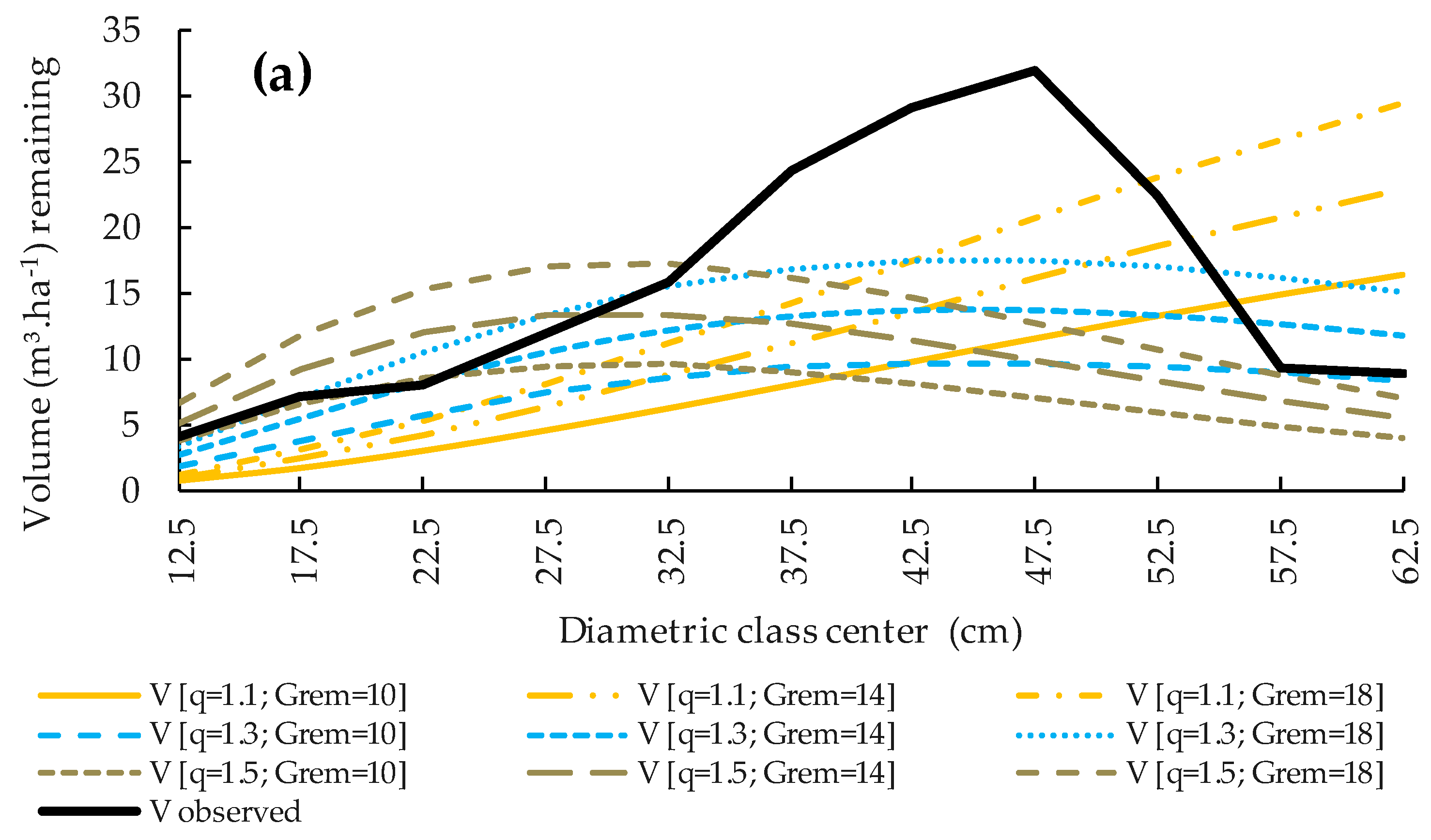
Figure 1. Distribution of observed and adjusted frequencies for A. angustifolia (Bertol.) Kuntze, aiming at the sustainability concept proposed by Liocourt’s law, in diametric classes, considering a remaining basal area of 10.0, 14.0, and 18.0 m2∙ha−1; and changing Liocourt’s quotient to 1.1, 1.3, 1.5.
Forests 11 00339 g001
Figure 2. Adjusted equation for the annual percentage of volume increments up to the crown, with bark (PAI%vtci), (a) and graphical analysis of the residues showing a regular distribution (b) of A. angustifolia (Bertol.) Kuntze.
Forests 11 00339 g002
Figure 3. Remaining volume and cutting behavior per hectare for different scenarios, with varying Liocourt’s quotient (q = 1.1, 1.3, 1.5) (a) and remaining basal area (Grem = 10.0, 14.0, 18.0) (b) for A. angustifolia (Bertol.) Kuntze in the Araucaria Forest in Lages, SC.
Forests 11 00339 g003aForests 11 00339 g003b
Table 1. Simulation of different scenarios, varying the values of Liocourt’s quotient (q = 1.1, 1.3, 1.5) and of the remaining basal area (Grem = 10.0, 14.0, 18.0), aiming at the sustainable management of A. angustifolia (Bertol.) Kuntze in Lages, SC.
VariablesUnitsq = 1.1q = 1.3q = 1.5
Gremm2·ha−110.014.018.010.014.018.010.014.018.0
Vrm3∙ha−189.3125.0160.782.8116.0149.176.4107.0137.5
ccyears27.213.22.830.316.35.933.619.79.3
CI%48.127.36.651.832.613.355.637.820.0
Rate Cutm3∙ha−182.747.011.389.156.022.995.665.034.4
Totalm3∙83.5 ha−16907.73926.7945.77442.84675.91908.97980.15428.12876.0
Where: Grem = remaining basal area, m2∙ha−1; Vr = remaining volume, m3∙ha−1; cc = cutting cycle in years; CI = cutting intensity in %; q = Liocourt’s quotient.
Table 2. Simulation of activities in the observed/remaining stand, and of the cuts to be performed according to the wood assortment classification, with Liocourt’s quotient (q) = 1.3, remaining basal area (Grem) = 14 m2·ha−1, and maximum desired diameter = 62.5 cm, for A. angustifolia (Bertol.) Kuntze in Lages, SC.
Center of the Class Diameter (CC)Observed Forest StandRemaining Forest StandCut Assortments
hichVS1VS2VS3VS4Vtci
N∙ha−1G∙ha−1V∙ha−1N∙ha−1G∙ha−1V∙ha−1N∙ha−1G∙ha−1V∙ha−1(m)(m)n%n%n%(m3∙cc)%(m3∙cc)
12.5810.99404.1520.63392.6300.36011.55.49.000.000.000.00.0503100.00.0503
17.5521.25077.0400.95575.4120.29511.78.111.900.000.000.00.1351100.00.1351
22.5301.19287.9311.21528.100.00000.09.913.900.000.0132.30.178967.70.2644
27.5271.603712.0241.396410.440.20721.611.115.300.000.0372.10.122927.90.4406
32.5241.991015.7181.500312.050.49073.712.016.400.0133.6353.00.089013.40.6656
37.5262.871624.2141.536513.1121.335111.112.717.300.0256.4340.80.02622.80.9408
42.5233.262829.0111.518113.6121.744715.413.318.000.0373.6223.50.03722.91.2674
47.5193.366931.881.458713.6111.908218.213.718.6152.5346.900.00.00970.61.6466
52.5112.381222.361.370813.241.01059.114.119.1151.1346.800.00.04372.12.0796
57.541.03879.251.264812.500.00000.014.419.5283.9112.700.00.08713.42.5674
62.530.92048.941.149511.700.00000.014.719.8282.7112.800.00.14074.53.1112
67.520.71578.031.031410.700.00000.014.920.1281.6112.900.00.20485.53.7121
70.010.38485.830.972810.200.00000.015.020.3281.1113.000.00.24116.04.0343
Total *30020.9172.021114.0116.0917.462.3
Where: CC = center of diameter class at breast height in cm; N∙ha−1 = number of trees per hectare; V∙ha−1 = volume per hectare; G∙ha−1 = basal area per hectare; hic = increments up to the crown, in m; h = total height, in m; Total* = total value for the desired center of 62.5 cm; VS1, VS2, VS3 = rate of the volume of each assortment up to Vtci in relation to the total, in%; VS4 = residual volume of the last section with stem, in m3∙cc; Vtci = total volume increments up to the crown, in m3∙cc.

