Article

Demonstrating the Effect of Height Variation on Stand-Level Optimization with Diameter-Structured Matrix Model

1
Faculty of Sciences, University of Oulu, FI-90014 Oulu, Finland
2
Natural Resource Institute Finland (Luke), FI-90014 Oulu, Finland
*
Author to whom correspondence should be addressed.
Forests 2020, 11(2), 226; https://doi.org/10.3390/f11020226
Submission received: 18 December 2019 / Revised: 11 February 2020 / Accepted: 13 February 2020 / Published: 18 February 2020
(This article belongs to the Section Forest Inventory, Modeling and Remote Sensing)

Abstract

:
The weakness of the population matrix models is that they do not take into account the variation inside the class. In this study, we introduce an approach to add height variation of the trees to the diameter-structured matrix models. In this approach, a new sub-model that describes the height growth of the trees is included in the diameter-structured model. We used this height- and diameter-structured matrix model to maximize the net present value (NPV) for the remaining part of the ongoing rotation for Scots pine (Pinus sylvestris L.) stand and studied how the height variation affects to the results obtained through stand-level optimization. In the optimization, the height variation was taken into account by setting the lower saw-log price for the short trees. The results show that including the height variation into the optimization reduced the financial outcome by 16–18% and considerably changed the structure of optimal management (e.g., timings for thinnings, rotation period and intensity of thinnings). We introduced an approach that can be applied to include not only height variation but also variation of other tree properties (such as branchiness or the amount of heartwood and sapwood) into the matrix models.

1. Introduction

Structured population models (either size-, stage- or age-structured) provide the connection between the population-level dynamics and individual level vital rates [1]. In brief, for stage- or age-structured populations a specific model is constructed to describe reproduction, growth and mortality [2] with the probabilities that population in one age or stage (size) class transfers to another between two sequential periods in time [3,4]. Growth is modeled as a transition from a class to upper classes, survival (opposite to mortality) as the cumulated transitions from a class to other classes and recruitment (reproduction) as a transition into the first class [5]. Particularly in forestry size-structured models (e.g., interchangeably transition matrix model, matrix population model, matrix growth model or matrix model) are thriving with applications covering a wide range of areas [6,7]. For instance, transition matrix models have been applied in discovering biodiversity dynamics [8], in studying the impacts of climate change [9], in biomass carbon stock studies (e.g., [10]) and in assessing optimal forest management [11,12,13,14]. For optimal forest management, there are also other approaches widely applied for predicting tree growth—such as process-based [15,16,17,18] and statistical-empirical growth models [19,20,21]. One argument favoring matrix models over e.g., individual-based statistical–empirical models is the fact that they in most cases require distinctively less amount of information [22].
Despite the extensive application of matrix growth models they have been criticized for their inability to incorporate variation among the individuals consisting of a particular size or age category [23]. Since matrix models operate on size- (or age-, or stage-) structured populations differences among individuals due to size (age or stage) might be an incomplete predictor of actual growth [7]. Further, the outputs of the matrix models are sensitive to the dimension of the matrix, or equivalently to the width of the size classes. This dependence of elasticities on matrix dimensionality has been criticized to lead possible fast pathways which in turn may result in biologically and/or physically impossible growth rates [7]. However, there are methods to circumvent this problem [7]—nevertheless, they are tedious, and require more information which to some extent violate Occam’s razor principle to apply parsimonious models [24].
For modeling tree breeding with a matrix model, it is a problem that variation between individuals within the same size (age or stage) class is not taken into account. Namely, a recent study [25] suggests that branch properties (i.e., branch angle, branch thickness and branch multiplicity) are statistically significantly better in improved trees (i.e., genetically improved by tree breeding methods) than in unimproved trees. However, there is considerable variation between individuals. Stated differently, valuable branch traits (flat branch angle, thin branches and fewer branches in a whorl) are more common with improved material than with unimproved, and this can further be converted into monetary value [26]. Currently, more studies focusing on combining branch traits with lumber grading and further pricing [27,28] are called for. Further, more research on branch characteristics associated with unimproved and improved seed material [29,30], and their effect on timber grade distribution is needed. However, before such results exist, one can estimate the effect of fluctuating tree characteristics on financial performance by conducting simulations.
This study introduces an approach that enables us to take into account the height variation between individuals within a particular diameter class in population matrix models. It applies state constrained optimal control problems related to forest management. The state is described with a diameter-structured population matrix model, where is included the new sub-model describing the height growth of the trees. The computational methods of this research are based on the numerical methods of nonlinear, constrained optimization and differential equations, which previously followed by Pyy et al. [14]. The main aim of the study is to demonstrate possible effects of height variation on financial performance when a diameter-structured matrix model is applied in stand-level optimization.

2. Material and Methods

2.1. The Optimization Problem

Typically, the optimization helps in solving the forest stand management policy that maximize the net present value (NPV) of the ongoing rotation. In order to formulate the control problem we define the following notations. We divided trees into non-overlapping diameter and height classes with uniform class widths Δ x and Δ z , respectively. The diameter of the trees in the diameter class i = 1 , , N is denoted by x i and the height of the trees in the height class j = 1 , , K by z j . Time was divided into subintervals [ t k 1 , t k ) , k = 1 , , M , with the length of the time step Δ t . We denoted a tree in the diameter class i and the height class j tree ( i , j ) . Denoting number of trees ( i , j ) and number of removed trees ( i , j ) per unit area at time step k by y i j k and h i j k , respectively. We denoted y k = ( y 11 k , , y 1 K k , y 21 k , , y 2 K k , , y N 1 k , , y N K k ) and h k = ( h 11 k , , h 1 K k , h 21 k , , h 2 K k , , h N 1 k , , h N K k ) . By y and h are denoted vectors ( y 1 , , y M ) and ( h 1 , , h M 1 ) , respectively.
The optimization problem is in form
max ( y , h ) Y × H J ( y , h ) : = i = 1 N j = 1 K k = 1 M 1 w i j k h i j k + w i j M y i j M ,
where w i j k is the discounted revenues of a tree ( i , j ) at time step k. The clearcut is done at time step M. We solved the optimization problem with different values of M (time step Δ t remains same so final time t M changes) and chose that which gave the maximal value for the problem (1). Every tree is divided into two quality classes: saw log and pulpwood denoted by subindexes q = 1 and q = 2 , respectively. Further, if the height of a tree in diameter class i, is less than μ i 0.5 m then the unit price of the saw log for the tree is lower than the original saw log price, where μ i denotes the mean height of the diameter class i. Technically, the term μ i 0.5 m is a sanction which degrades the saw log price for trees which are shorter (by 0.5 m) than the mean height of the particular diameter class i. The rationale is that the smaller the tree the less allowance there is for bucking, which in turn has a negative effect on a saw log price [31]. In this connection it should be highlighted that although the height variation does not have a direct correspondence to wood quality it has bearing on the saw log recovery. The discounted price is
w i j k = 1 ( 1 + r ) t k ( c ˜ 1 V i j 1 + c 2 V i j 2 ) if z j < μ i 0.5 m 1 ( 1 + r ) t k ( c 1 V i j 1 + c 2 V i j 2 ) else ,
where V i j q is the volume of that part of the tree ( i , j ) that belongs to quality class q, c 1 and c 2 are the price of saw log and pulpwood per volume, respectively, and c ˜ 1 is the saw log price for trees shorter than μ i 0.5 m. Technically, three alternative unit prices for saw logs were applied for trees shorter than μ i 0.5 m. The applied unit prices were: (a) c ˜ 1 = c 1 , (b) c ˜ 1 = 0.8 c 1 and (c) c ˜ 1 = c 2 . Price for saw logs ( c 1 ) was 58.44 €m 3 and for pulpwood ( c 2 ) 16.56 €m 3 .
State y k depends on number of removed trees h k via matrix population model [13]
(3) y k + 1 = A k y k h k + 1 , k = 0 , , M 1 , (4) y 11 k = R k , k = 1 , , M (5) y 0 = y 0 ,
where R k is number of new trees at time step k and y 0 is a size distribution of trees at time t 0 . The sets of constraints for y and h are
Y = { y | y 0 : y is a solution for Equations ( 3 ) ( 5 ) } ,
H = { h | 0 h h m a x : | | h k | | 1 B or h k = 0 , k = 1 , , M 1 } ,
respectively, where h m a x is the upper limit of removed trees and B = 50 m 3 ha 1 denotes the lower limit of making a thinning at time step k.
The matrix A k is in form
A k = a 1 k H 0 0 0 b 1 k H a 2 k H 0 0 0 0 b N 1 k H a N k H ,
where 0 a i k 1 , i = 1 , , N , and 0 b i k 1 , i = 1 , , N 1 , k = 1 , , M . The coefficients a i k and b i k are assumed to depend on basal area P k = i = 1 N π x i 2 2 y i k of the stand. The details about model was described by Pyy et al. [13]. The matrix H is a K × K -matrix that describes how the trees move from a height class to another. We wanted to choose a small height class width Δ z so we assumed that trees from the height class j can remain in the same class or grow to every upper height class j ( j j ). So the matrix H is in form
H = e 11 0 0 e 21 e 22 0 e K 1 e K 2 e K K ,
where 0 e j j 1 , j , j = 1 , , K are proportions of trees that move from the height class j to the height class j . We assumed that H does not depend on time step k or diameter class i. The parameters are fitted on the data described in Section 2.2 below followed by other study [13]. The projected gradient method was used to solve the optimization problem (1) in accordance with other study [14].

2.2. Model Estimation and Data

The data used to estimate the parameters for the population model were derived from two long-term experiments (i.e., HARKAS series; for detail see, e.g., [32]). The two experiments were established in the 1978 and 1984 in even-aged, pure commercial Scots pine (Pinus sylvestris L.) stands located on mineral soil in Muhos municipality, Ostrobothnia region, Finland (26°06′05″ E and 64°46′02″ N, asl 60–70 m). The data were based on 8 360 tree records from 20 sample plots. The stand management among the sample plots fluctuated considerably: from control plots (no thinnings) to very intensive thinnings (60% of the basal area removed). The stand age in the data set was on average 25 years, indicating that establishment costs and costs of precommercial thinning are sunk. Further, we did not apply any modeling for the time period between stand establishment and 25 years.
We fitted the tree height data (2205 trees, heights between 2.7 m and 19.3 m) to follow Näslunds height curve [33]
x z 1.3 = b 0 + b 1 x
.
Parameters b 0 and b 1 were estimated by least-squares method. We assumed that at time t 0 height of the trees in the diameter class i follows normal distribution [33] with mean
μ i = x i 2 ( b 0 + b 1 x i ) 2 + 3 x i 2 ( b 0 + b 1 x i ) 4 σ 2 + 1.3
and standard deviation
s i = σ 2 ( μ i 1.3 ) 3 2 x i ,
where σ 2 is the variance of the variable x i z 1.3 .
The minimum diameter of quality class q is denoted by x m i n , q , q = 1 , 2 . For saw log x m i n 1 = 15 cm and for pulpwood x m i n 2 = 5.5 cm [28]. Let l i j q denote the height, where the tree ( i , j ) has the diameter x m i n , q . Then for the tree ( i , j ) , the saw log part is from ground to the height l i j 1 and pulpwood part from height l i j 1 to the height l i j 2 . The height l i j q = ( 1 s ) z j , where 0 s 1 . The unknown s was solved from the equation [34]
x m i n , q f ( s j ) x i = f ( s )
.
In the equation s j = 1 1.3 z j and f ( s ) is taper curve
f ( s ) = b 1 s + b 2 s 2 + b 3 s 3 + b 4 s 5 + b 5 s 8 + b 6 s 13 + b 7 s 21 + b 8 s 34 ,
where the form and the values for parameters b 1 , , b 8 were taken from [34]. We solved s from the Equation (13) by using MATLAB function SOLVE.
The volume of a tree ( i , j ) is
V i j = 1 1000 v 1 x i v 2 v 3 x i z j v 4 ( z j 1.3 ) v 5 ,
where the form and the values for parameters v 1 , , v 5 were taken from [34]. For a tree ( i , j ) the area under the taper curve (14) on the intervals ( 0 , z j ) , ( l i j 0 , l i j 1 ) and ( l i j 1 , l i j 2 ) are A i j 0 , A i j 1 and A i j 2 , respectively, where l i j 0 = 0 . Then the volume
V i j q = A i j q A i j 0 V i j
.
In the population model (3) the parameters a i and b i of the matrix A k were estimated similarly as in explicit approximation of continuous diameter structured population model (see [14]). The parameters e j j , j , j = 1 , , K , of matrix H were estimated with the proportion estimator [6]. The recruitment model (4) is based on the average stand conditions in the 7th National Forest Inventory [35]:
R k = 0 if k = 1 , , d P p i n e c B A k d ( S r e f S k d ) if k = d + 1 , , M ,
where P p i n e = 0.5581 is relative proportion of pines, S r e f = 4009.5 is average number of trees per hectare, S = i = 1 N j = 1 K y i j k is actual number of trees per hectare and d is number of time steps before the new trees are big enough to the first size class. Coefficient
c B A k = 0.01 + 0.2475 · B A k if B A k < 3.9 m 2 , 1.0 if 3.9 m 2 B A k < 8.0 m 2 , 1.471 0.05882 · B A k if 8.0 m 2 B A k < 25.0 m 2 , 0 if B A k 25.0 m 2 ,
describes the density effect at time step k as a function of stand basal area B A k .
Finally, in the simulations, the time step was set to 5 years with width of diameter class Δ x = 3 cm and width of the height class Δ z = 0.5 m. Minimum diameter and height were set to 2 cm and 2 m, respectively. Then, a minimum of 15-yr growth was assumed to new trees to achieve the first size class, d = 3 cm.

3. Results

The simulations revealed that height variation combined with pricing had a considerable effect on both financial performance as well as on the optimal management schedules (Table 1, Figure 1). For instance, when saw log unit price was set equal to pulpwood price for trees shorter than μ i 0.5 m the optimal rotation period was shortened. Especially when discounting with 4%, the optimal rotation period was shortened 20 years (Figure 1). Further, when discounting with 3%, the structure of thinnings changed drastically with saw logs price set to equal pulpwood price for trees shorter than μ i 0.5 m, compared to the other two price options (Table 1). The financial performance (expressed as maximum net present value, MaxNPV) decreased significantly, ranging from 16% to 18% (depending on the interest rate) when height variation with pricing was taken into account (Table 1). Regardless of the discount rate (3% or 4%) height variation with pricing shortened the optimal rotation period but also reduced the financial outcome. When sawlog unit price was set equal to pulpwood unit price the MaxNPV reduced 409–477 €. However, the impact of height variation and pricing to mean annual increment (associated with stand-level optimum) was minor: approximately 1% difference among the pricing options (Table 1).
As an example of how height variation develops in a diameter class, we will consider the case where the interest rate is 3% and the price of saw log for short trees is the price of saw log. Figure 2 presents the height variation at different time steps in diameter class 14–17 cm.

4. Discussion

Forest growth and yield models and optimization models are both needed in order to achieve the goals set for forest management [36]. There are, of course, several alternatives for both growth and yield models [37] and optimization models [36,38] to be applied. Currently, traditional empirical-statistical models have made way to e.g., process-based models [36] and to matrix models [6]. Despite the fact that matrix models have been applied to almost all subject areas of forestry [6], they have been criticized for their inability “to incorporate variation among individuals within a size category” [7]. This deficiency associated with matrix models is particularly troublesome regarding tree breeding since it has recently been shown that improved reforestation material tends to have a different distribution with respect to e.g., wood properties (such as branchiness) than unimproved material [25]. Since distributional properties are likely to be different among improved and unimproved reforestation material, this leads to a question of whether that might have an impact on financial performance as well. To study this, the constraint of homogeneity associated with individuals within a particular size category (cf. [2]) needed first to be relaxed. The main objective of this study was to introduce a variation between individuals into a matrix model, and further to demonstrate its effect on financial performance assessed according to stand-level optimization (cf. [39]).
Technically, the height variation between individuals was included in the financial analysis (stand-level optimization) by setting a penalty. In brief, a tree shorter than an arithmetic average tree height within a size category was labeled with a lower unit price of saw logs. The rationale was that the shorter the tree the less allowance there is for bucking, which in turn has a negative effect on a saw log price [31]. Our results indicated that including variation into the matrix model has a notable impact on financial performance. Interestingly, the MaxNPV changed by approximately 16–18% when height variation with pricing was included in stand-level optimization. Although the variation was here set to tree height (and further linked to saw log pricing by specific penalty function), it does not matter which variation is eventually included in the matrix model. One can choose variation in any stem property, for instance branchiness [40] as long as the variation can be linked to financial valuing. Further, the ideal case would be to include variation in some of the key indicators of timber quality—such as the size and type of knots or the amount of heartwood and sapwood [37]—into the matrix model, and to examine this effect in monetary terms with and without the genetic gains [26]. However, such an analysis strongly depends on available data sets, and thus it is conditional to status quo—whether such data had been gathered until now or not.
Finally, it should bear in mind that this study excludes any consideration of sustainability (cf. [41]) or ecosystem services (cf. [10]), solely focusing on the financial performance of timber production. Since this study introduces a new method to include the variation between individuals in a matrix model, and further to assess it in monetary value, the authors consider this contribution to be the first step, and further steps in the near future would cover more than merely timber production.

5. Conclusions

Including height variation of trees in a diameter-structured matrix model changes the optimal solutions compared to the case without height variation. Differences (with respect to rotation period and intensity as well as the timing of thinnings) are clear, regardless of the applied discount rate. This simply indicates that variations in tree characteristics (e.g., in-branch traits) within the same size class needs to be taken into account more systematically than has been done earlier in population matrix models (e.g., [7]). The approach used in this study enables including any property relevant to timber grading and further pricing and maximizing financial performance.

Author Contributions

Conceptualization A.A.; methodology and software J.P.; formal analysis A.A.; supervision E.L. and A.A.; writing—original draft preparation J.P. and A.A.; writing—review and editing J.P., E.L. and A.A. All authors have read and agreed to the published version of the manuscript.

Funding

This research received no external funding.

Conflicts of Interest

The authors declare no conflict of interest.

References

  1. Xie, Q.; He, Z.-R.; Wandg, X. Optimal harvesting in diffusive population models with size random growth and distributed recruitment. Electron. J. Differ. Eq. 2016, 214, 1–13. [Google Scholar]
  2. Goetz, R.U.; Xabadia, A.; Calvo, E. Optimal forest management in the presence of intraspecific competition. Math. Popul. Stud. 2016, 18, 151–171. [Google Scholar] [CrossRef]
  3. Lefkovitch, L. The study of population growth in organisms grouped by stages. Biometrics 1965, 21, 1–18. [Google Scholar] [CrossRef]
  4. Caswell, H. Matrix Population Models: Construction, Analysis and Interpretation, 2nd ed.; Sinauer Associates Inc.: Sunderland, MA, USA, 2001. [Google Scholar]
  5. Picard, N.; Mortier, F.; Chagneau, P. Influence of estimations of the vital rates in the stock recovery rate using matrix models for tropical rainforests. Ecol. Model. 2008, 214, 349–360. [Google Scholar] [CrossRef]
  6. Liang, J.; Picard, N. Matrix model of forest dynamics: An overview and Outlook. For. Sci. 2013, 59, 359–378. [Google Scholar] [CrossRef]
  7. Picard, N.; Liang, J. Matrix models for size-structured populations: Unrealistic fast growth or simply diffusion? PLoS ONE 2014, 9, e98254. [Google Scholar] [CrossRef]
  8. Liang, J.; Zhou, M. A geospatial model of forest dynamics with controlled trend surface. Ecol. Model. 2010, 221, 2339–2352. [Google Scholar] [CrossRef]
  9. Liang, J.; Zhou, M.; Verbyla, D.; Zhang, L.; Springsteen, A.L.; Malone, T. Mapping forest dynamics under climate change: A matrix model. For. Ecol. Manag. 2011, 262, 2250–2262. [Google Scholar] [CrossRef]
  10. Hu, H.; Wang, S.; Guo, Z.; Xu, B.; Fang, J. The stage-classified matrix models project a significant increase in biomass carbon stocks in China’s forests between 2005 and 2050. Sci. Rep. 2015, 5, 11203. [Google Scholar] [CrossRef] [Green Version]
  11. Pihlainen, S.; Tahvonen, O.; Niinimäki, S. The economics of timber and bioenergy production and carbon storage in Scots pine stands. Can. J. For. Res. 2014, 44, 1091–1102. [Google Scholar] [CrossRef]
  12. Assmuth, A.; Rämö, J.; Tahvonen, O. Economics of size-structured forestry with carbon storage. Can. J. For. Res. 2018, 48, 11–22. [Google Scholar] [CrossRef] [Green Version]
  13. Pyy, J.; Ahtikoski, A.; Laitinen, E.; Siipilehto, J. Introducing a Non-Stationary Matrix Model for Stand-Level Optimization, an Even-Aged Pine (Pinus sylvestris L.) Stand in Finland. Forests 2017, 8, 163. [Google Scholar] [CrossRef] [Green Version]
  14. Pyy, J.; Ahtikoski, A.; Lapin, A.; Laitinen, E. Solution of Optimal Harvesting Problem by Finite Difference Approximations of Size-Structured Population Model. Math. Comp. Appl. 2018, 23, 22. [Google Scholar] [CrossRef] [Green Version]
  15. Cao, T.; Valsta, L.; Mäkelä, A. A comparison of carbon assessment methods for optimizing timber production and carbon sequestration in Scots pine stands. For. Ecol. Manag. 2010, 260, 1726–1734. [Google Scholar] [CrossRef]
  16. Niinimäki, S.; Tahvonen, O.; Mäkelä, A. Applying a process-based model in Norway spruce management. For. Ecol. Manag. 2012, 265, 102–115. [Google Scholar] [CrossRef]
  17. Tahvonen, O.; Pihlainen, S.; Niinimäki, S. On the economics of optimal timber production in boreal Scots pine stands. Can. J. For. Res. 2013, 43, 719–730. [Google Scholar] [CrossRef]
  18. Hurttala, H.; Cao, T.; Valsta, L. Optimization of Scots pine (Pinus sylvestris) management with the total net return from the value chain. J. For. Econ. 2017, 28, 1–11. [Google Scholar] [CrossRef]
  19. Pohjola, J.; Valsta, L. Carbon credits and management of Scots pine and Norway spruce stands in Finland. For. Policy Econ. 2007, 9, 789–798. [Google Scholar] [CrossRef]
  20. Ahtikoski, A.; Salminen, H.; Ojansuu, R.; Hynynen, J.; Kärkkäinen, K.; Haapanen, M. Optimizing stand management involving the effect of genetic gain: Preliminary results for Scots pine in Finland. Can. J. For. Res. 2013, 43, 1–7. [Google Scholar] [CrossRef]
  21. Juutinen, A.; Ahtikoski, A.; Lehtonen, M.; Mäkipää, R.; Ollikainen, M. The impact of a short-term carbon payment scheme on forest management. For. Policy Econ. 2018, 90, 115–127. [Google Scholar] [CrossRef]
  22. Grimm, V. Ten years of individual-based modelling in ecology: What have we learned and what could we learn in the future? Ecol. Model. 1999, 115, 129–148. [Google Scholar] [CrossRef]
  23. Zuidema, P.A.; Jonsegas, E.; Chien, P.D.; During, H.J.; Schieving, F. Integral projection models for trees: A new parametrization method and a validation of model output. J. Ecol. 2010, 98, 345–355. [Google Scholar] [CrossRef]
  24. Sable, S.E.; Rose, K.A. A comparison of individual-based and matrix projection models for simulating yellow perch population dynamics in Oneida Lake, New York, USA. Ecol. Model. 2008, 215, 105–121. [Google Scholar] [CrossRef]
  25. Haapanen, M.; Hynynen, J.; Ruotsalainen, S.; Siipilehto, J.; Kilpeläinen, M.-L. Realised and projected gains in growth, quality and simulated yield of genetically improved Scots pine in southern Finland. Eur. J. For. Res. 2016, 135, 997–1009. [Google Scholar] [CrossRef]
  26. Ahtikoski, A.; Haapanen, M.; Hynynen, J.; Karhu, J.; Kärkkäinen, K. Genetically improved reforestation stock provides simultaneous benefits for growers and a sawmill, a case study in Finland. Scand. J. For. Res. 2018, 33, 484–492. [Google Scholar] [CrossRef]
  27. Lyhykäinen, H.T.; Mäkinen, H.; Mäkelä, A.; Pastila, S.; Heikkilä, A.; Usenius, A. Predicting lumber grade and by-product yields for Scots pine trees. For. Ecol. Manag. 2009, 258, 146–158. [Google Scholar] [CrossRef]
  28. Ojansuu, R.; Mäkinen, H.; Heinonen, J. Including variation in branch and tree properties improves timber grade estimates in Scots pine stands. Can. J. For. Res. 2018, 48, 542–553. [Google Scholar] [CrossRef]
  29. Mäkinen, H. Effect of intertree competition on branch characteristics of Pinus sylvestris families. Scand. J. For. Res. 1996, 11, 129–136. [Google Scholar] [CrossRef]
  30. Gort, J.; Zubizarret-Gerendiain, A.; Peltola, H.; Kilpeläinen, A.; Pulkkinen, P.; Jaatinen, R.; Kellomäki, S. Differences in branch characteristics of Scots pine (Pinus sylvestris L.) genetic entries grown at different spacing. Ann. For. Sci. 2010, 67, 70. [Google Scholar] [CrossRef] [Green Version]
  31. Malinen, J.; Kilpeläinen, H.; Verkasalo, E. Validating the predicted saw log and pulpwood proportions and gross value of Scots pine and Norway spruce harvest at stand level by Most Similar Neighbour analyses and a stem quality database. Silva Fenn. 2018, 52. [Google Scholar] [CrossRef]
  32. Mäkinen, H.; Isomäki, A. Thinning intensity and growth of Scots pine stands in Finland. For. Ecol. Manag. 2004, 201, 311–325. [Google Scholar] [CrossRef]
  33. Siipilehto, J.; Kangas, A. Näslundin pituuskäyrä ja siihen perustuvia malleja läpimitan ja pituuden välisestä riippuvuudesta suomalaisissa talousmetsissä. MetsäTieteen Aikakauskirja 2015, 4, 215–236. [Google Scholar]
  34. Laasasenaho, J. Taper curve and volume functions for pine, spruce and birch. Commun. Lnst. For. Fenn. 1982, 108, 1–74. [Google Scholar]
  35. Hynynen, J.; Ojansuu, R.; Hökkä, H.; Siipilehto, J.; Salminen, H.; Haapala, P. Models for predicting stand development in MELA System. Metsäntutkimus laitoksen tiedonantoja. Finn. For. Res. Inst. Res. Pap. 2002, 835, 31–35. [Google Scholar]
  36. Xue, H.; Mäkelä, A.; Valsta, L.; Vanclay, J.K.; Cao, T. Comparison of population-based algorithms for optimizing thinnings and rotation using a process-based growth model. Scand. J. For. Res. 2019. [Google Scholar] [CrossRef] [Green Version]
  37. Mäkelä, A.; del Rìo, M.; Hynynen, J.; Hawkins, M.J.; Reyer, C.; Soares, P.; van Oijen, M.; Tomé, M. Using stand-scale forest models for estimating indicators of sustainable forest management. For. Ecol. Manag. 2012, 285, 164–178. [Google Scholar] [CrossRef] [Green Version]
  38. Pukkala, T. Population-based methods in the optimization of stand management. Silva Fenn. 2009, 43, 261–274. [Google Scholar] [CrossRef] [Green Version]
  39. Anita, S.; Arnautu, V.; Stefanescu, R. Numerical optimal harvesting for a periodic age-structured population dynamics with logistic term. Numer. Funct. Anal. Optim. 2009, 30, 183–198. [Google Scholar] [CrossRef]
  40. Ikonen, V.-P.; Kellomäki, S.; Peltola, H. Sawn timber properties of Scots pine as affected by initial stand density, thinning and pruning: A simulation based approach. Silva Fenn. 2009, 43, 411–431. [Google Scholar] [CrossRef] [Green Version]
  41. Lopez-Torres, I.; Perez, S.O.; Robredo, F.G.; Belda, C.F. Optimizing the management of uneven-aged Pinus nigra stands between two stable positions. iFor. Biosci. For. 2016, 9, 599–607. [Google Scholar] [CrossRef] [Green Version]
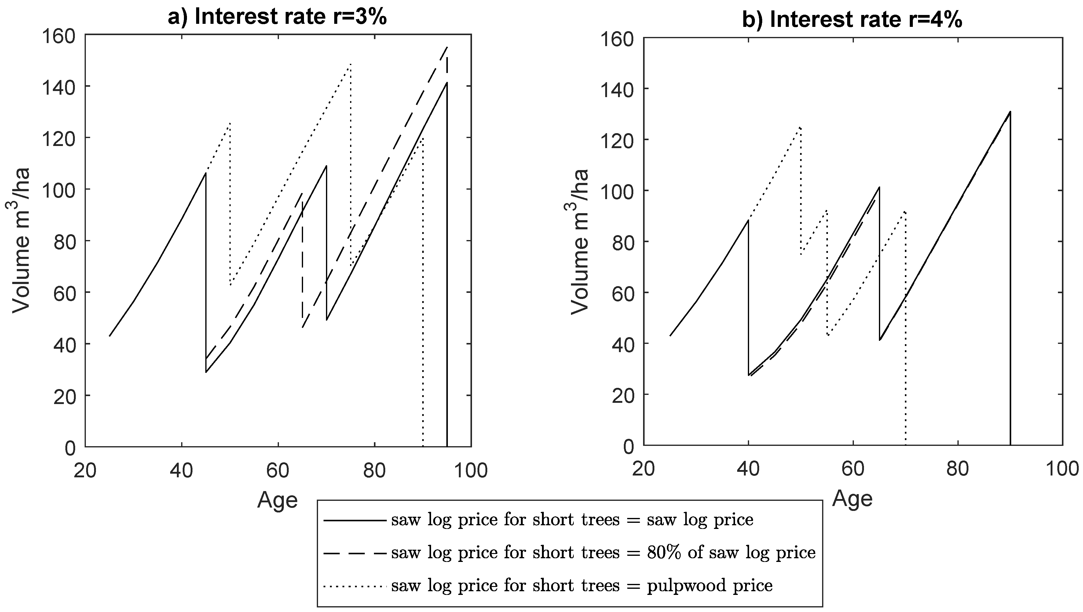
Figure 1. Volumes in stand managements with different saw logs pricing, m 3 /ha.
Forests 11 00226 g001
Figure 2. Height variation in diameter class 14–17 cm evolving in time, when stand management is optimized with 3% discount rate. On y-axis is number of stems (per hectare) and on x-axis height (in meters, m).
Forests 11 00226 g002
Table 1. Optimal stand-level managements when initial stand density is 1000 stems ha 1 (seeded trees).
ThinningStand Age (a)Removal (m 3 ha 1 )Thinning Intensity (% of Basal Area Removed)Saw Log Proportion (%)MaxNPV (€ha 1 )MAI (m 3 ha 1 a 1 )
c ˜ 1 c 1 / 0.8 c 1 / c 2 c 1 / 0.8 c 1 / c 2 c 1 / 0.8 c 1 / c 2 c 1 / 0.8 c 1 / c 2 c 1 / 0.8 c 1 / c 2 c 1 / 0.8 c 1 / c 2
Interest rate r = 3 %
1st45/45/5077.3/72.1/62.954/50/3560/61/673059/2872/25822.93/2.94/2.90
2nd70/65/7559.8/52.3/78.533/27/4264/64/72
clearcut95/95/90141.4/155.1/120.0100/100/10039/42/50
total 278.5/279.5/261.4 50/51/61
Interest rate r = 4 %
1st40/40/5060.9/61.9/50.661/62/2853/52/712169/2036/17602.80/2.79/2.76
2nd65/65/5560.1/58.4/50.032/31/3264/64/60
clearcut90/90/70131.0/130.5/92.4100/100/10035/35/38
total 252.0/250.9/193.0 46/46/52

