Feature-Level Fusion between Gaofen-5 and Sentinel-1A Data for Tea Plantation Mapping


Abstract
:1. Introduction
2. Materials and Methods
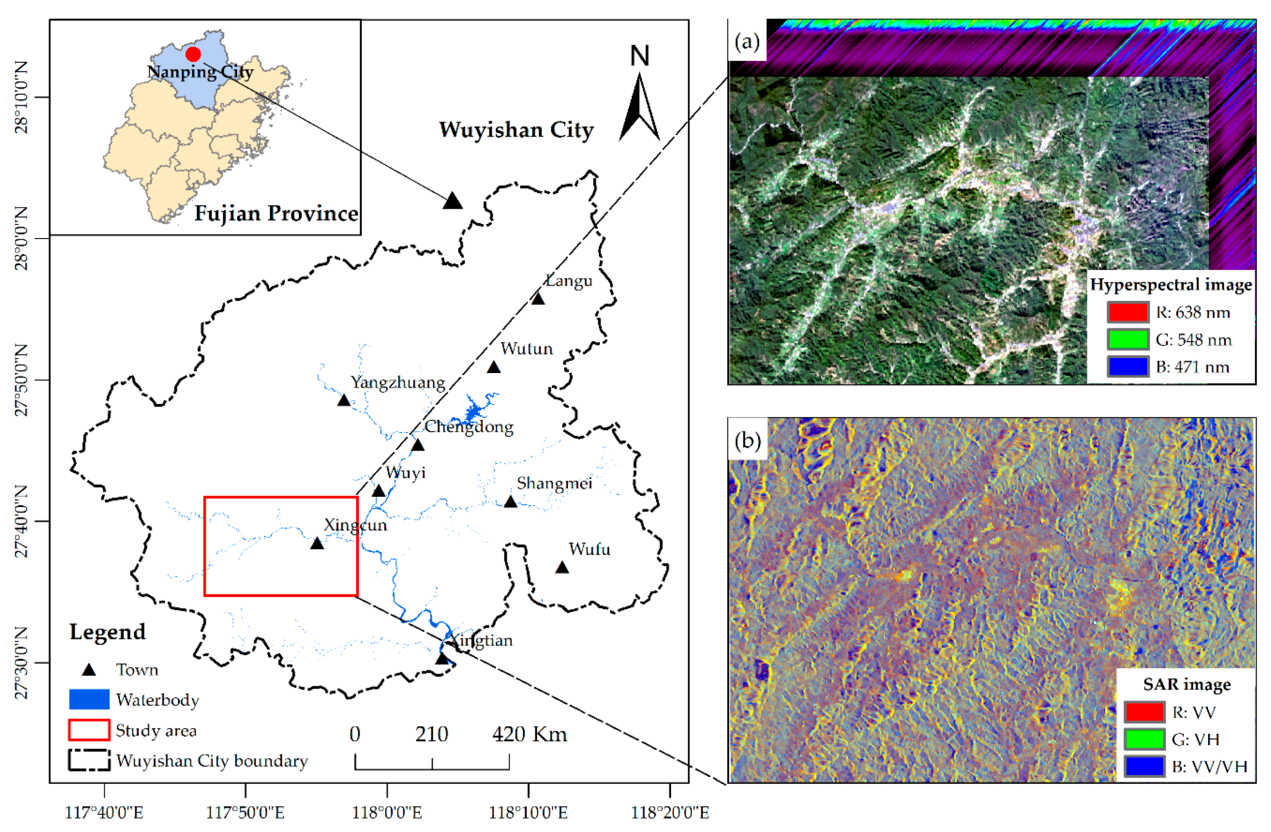
2.1. Study Area
2.2. Data Source
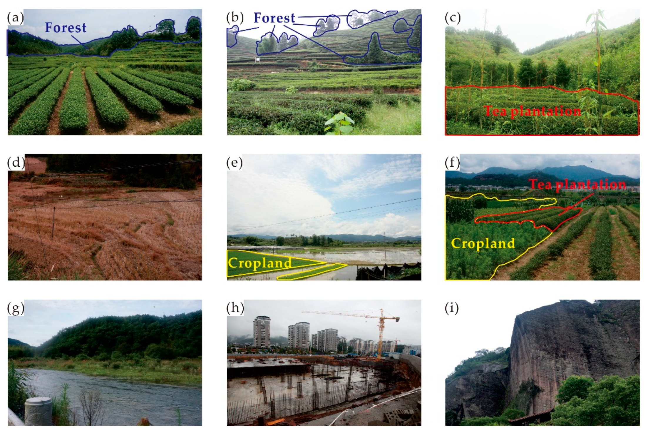
2.2.1. Field Survey
2.2.2. Remote Sensing and Auxiliary Data
2.3. Data Preprocessing
2.3.1. Hyperspectral Data Preprocessing
2.3.2. SAR Data Preprocessing
2.4. Feature Extraction
2.4.1. Principal Component Analysis
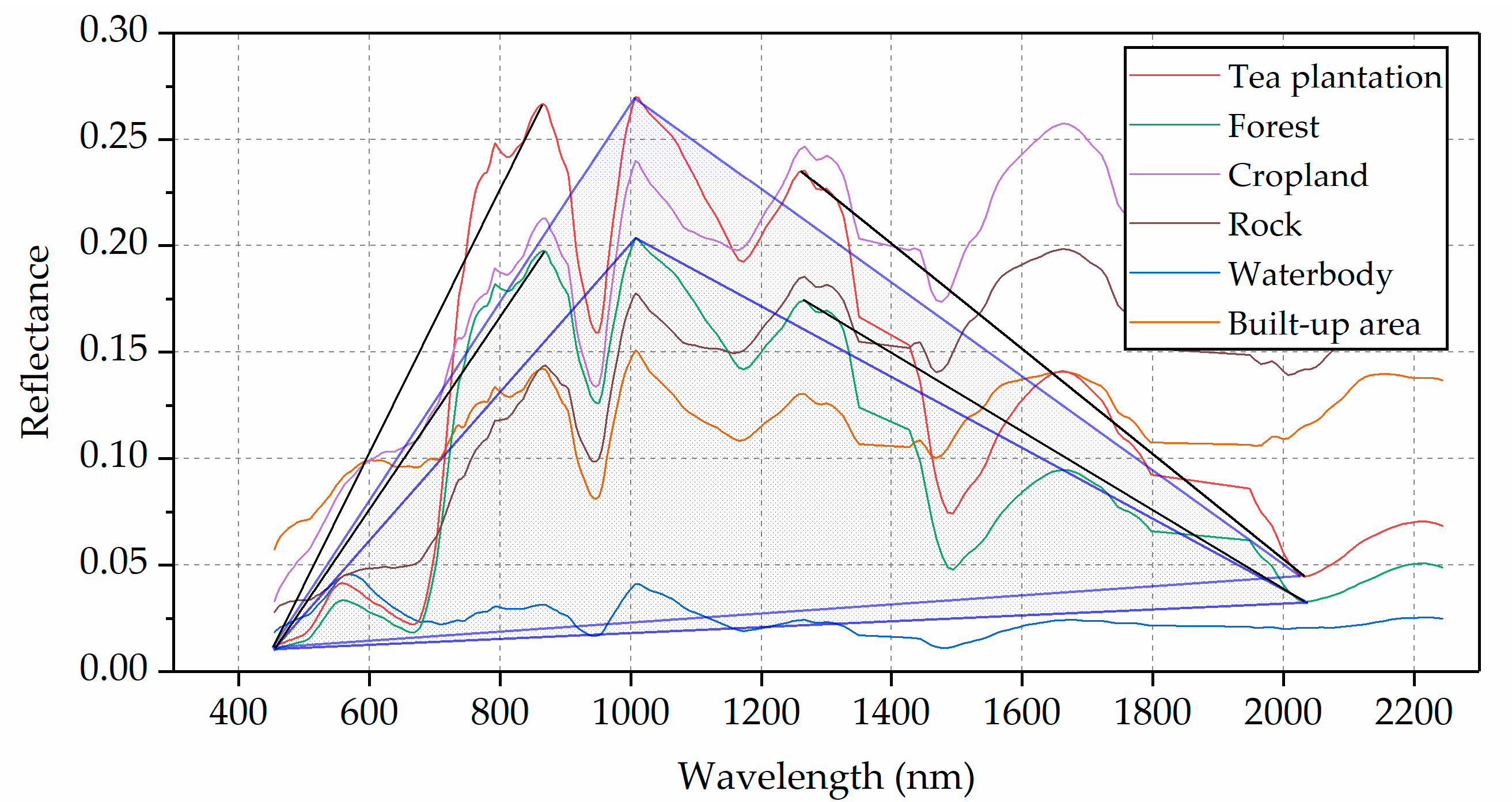
2.4.2. Spectral Index
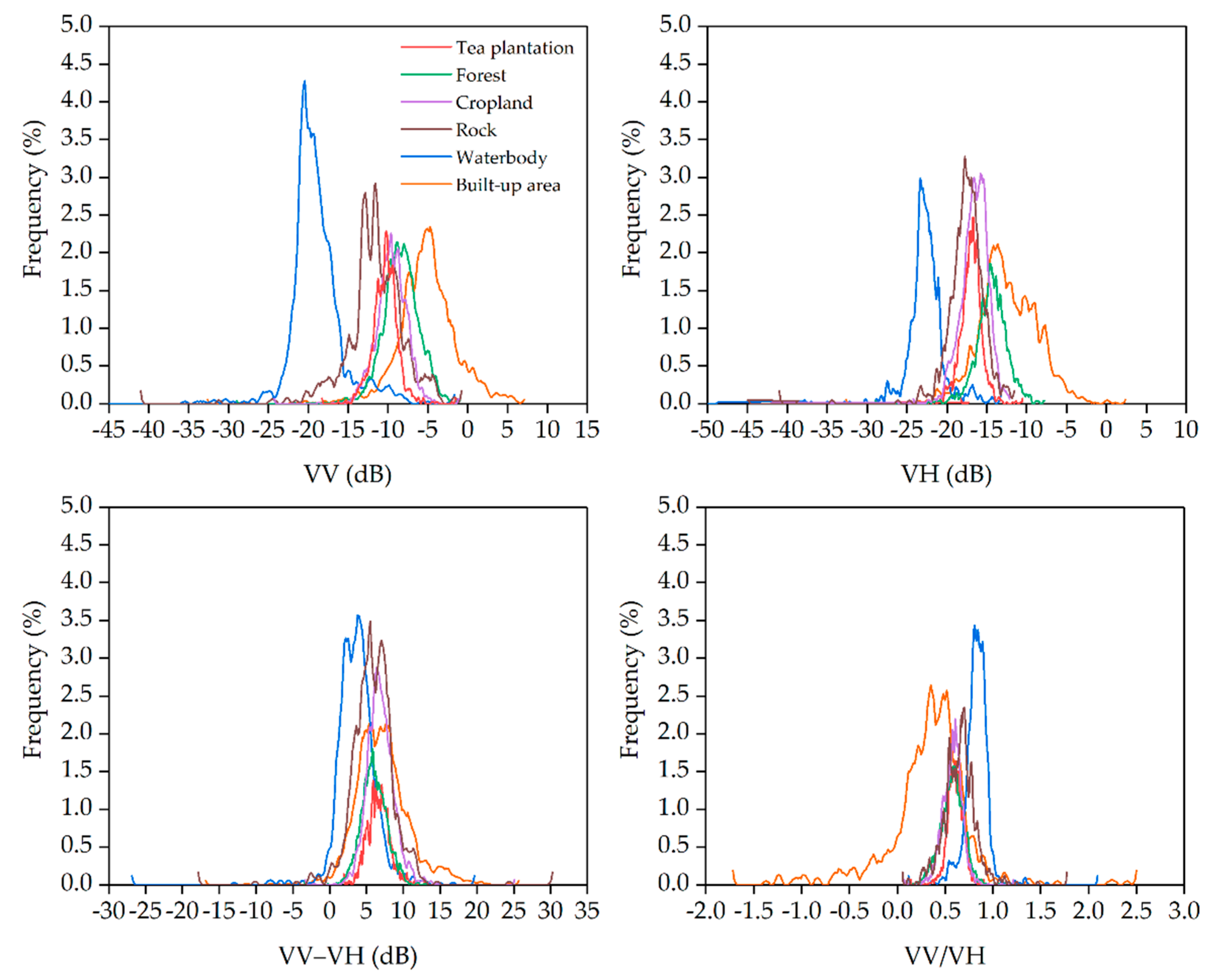
2.4.3. Polarimetric Feature
2.4.4. Spatial Feature
2.5. Image Fusion
2.5.1. Subspace Fusion (SubFus)
2.5.2. Combination of Locality Preserving Projection and SubFus
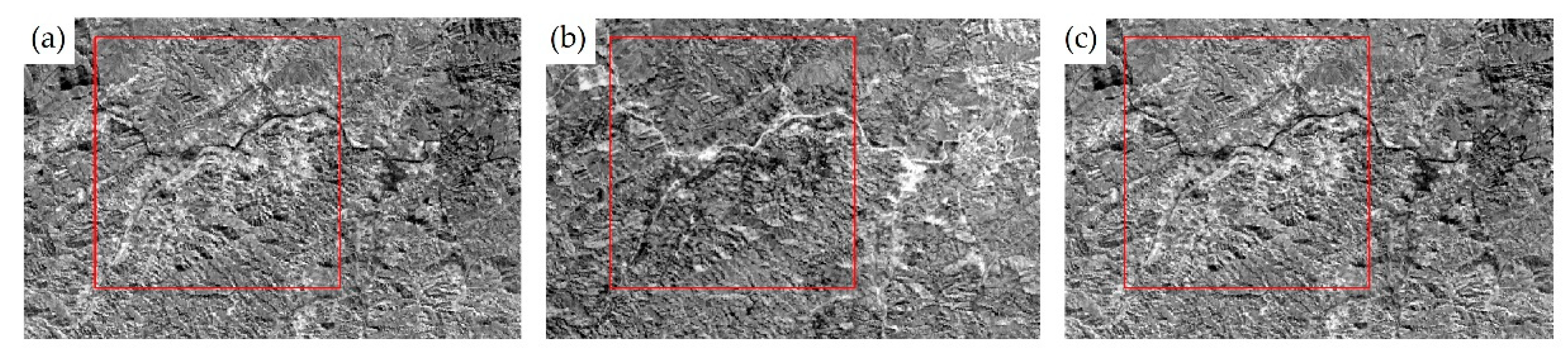
2.5.3. Pixel-Level Image Fusion
2.6. Image Classification
2.6.1. Classification Algorithm
2.6.2. Classification Scenario and Sample
2.6.3. Parameter Setting and Accuracy Assessment
3. Results
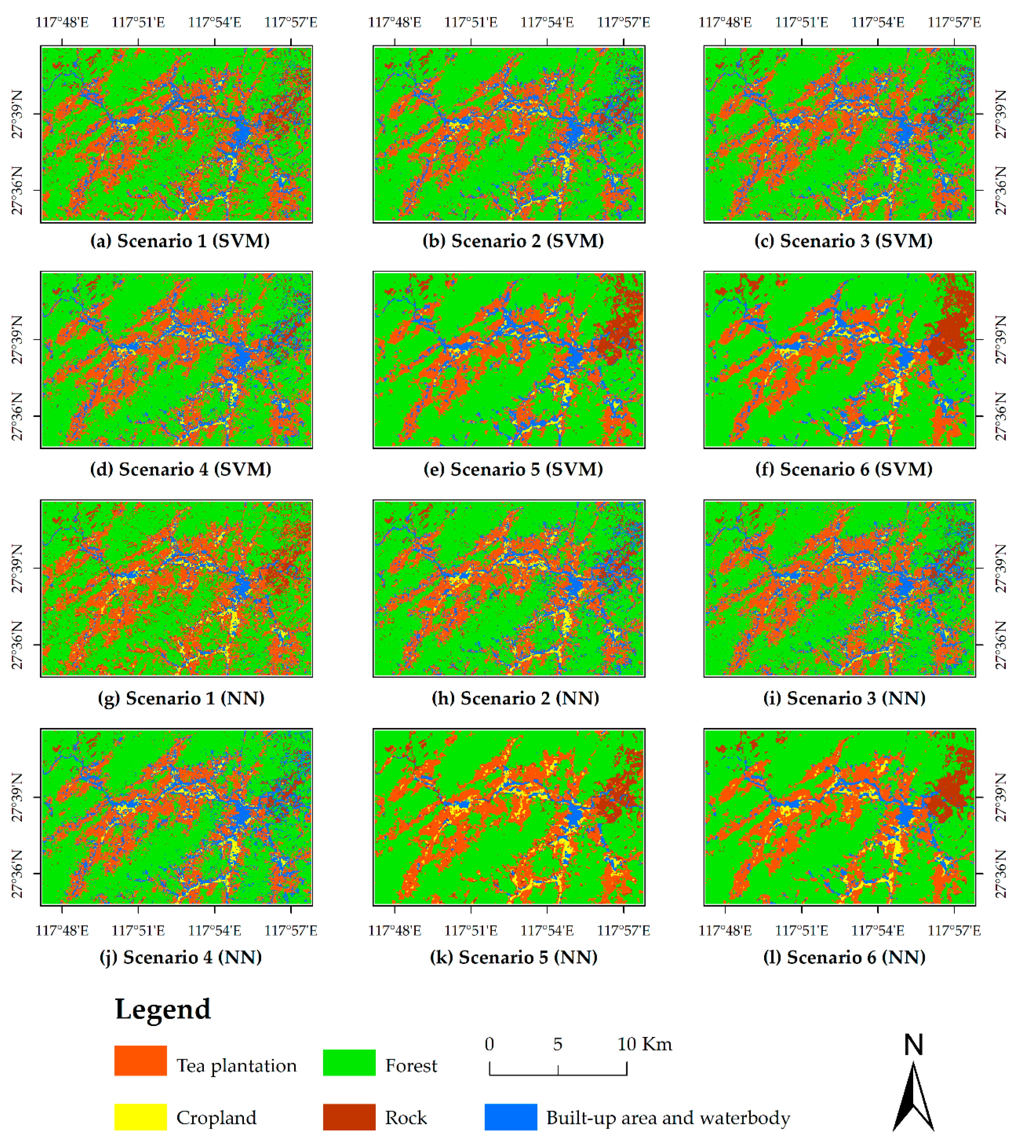
3.1. Visual Comparison of Thematic Maps
3.2. Comparison of Classification Accuracy
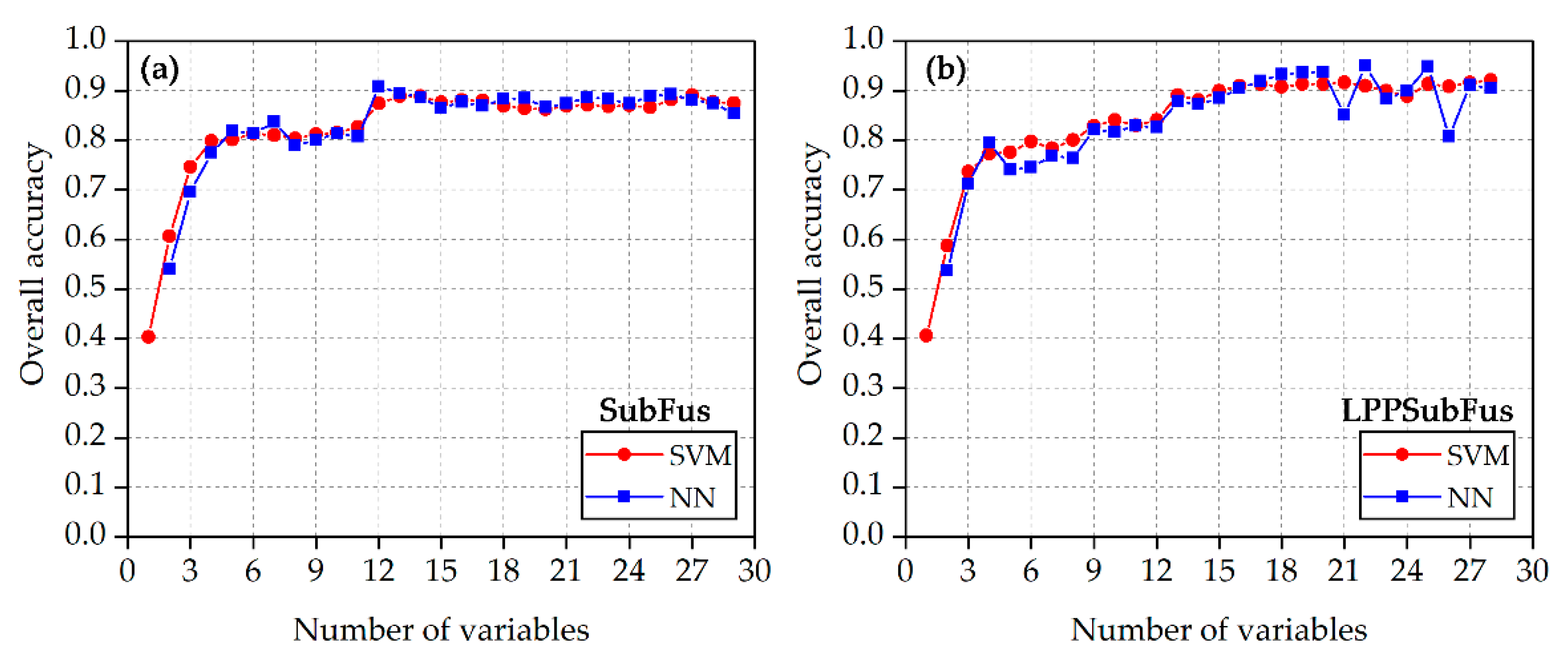
3.2.1. Comparison of Overall Accuracy
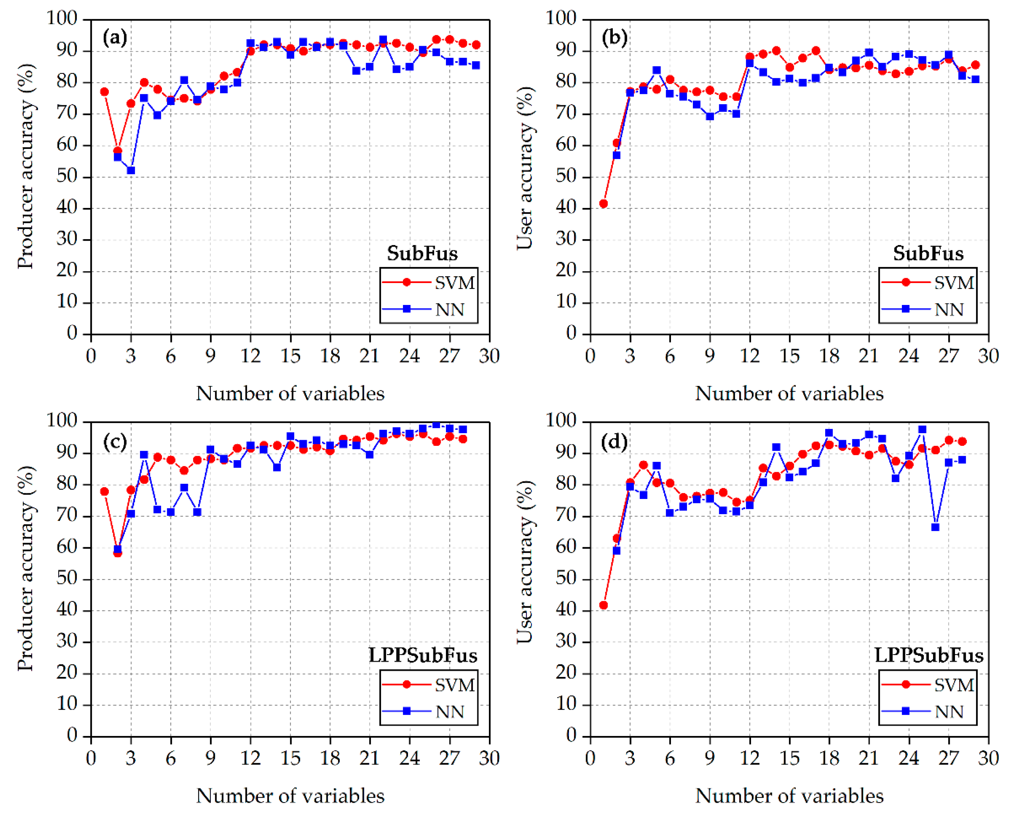
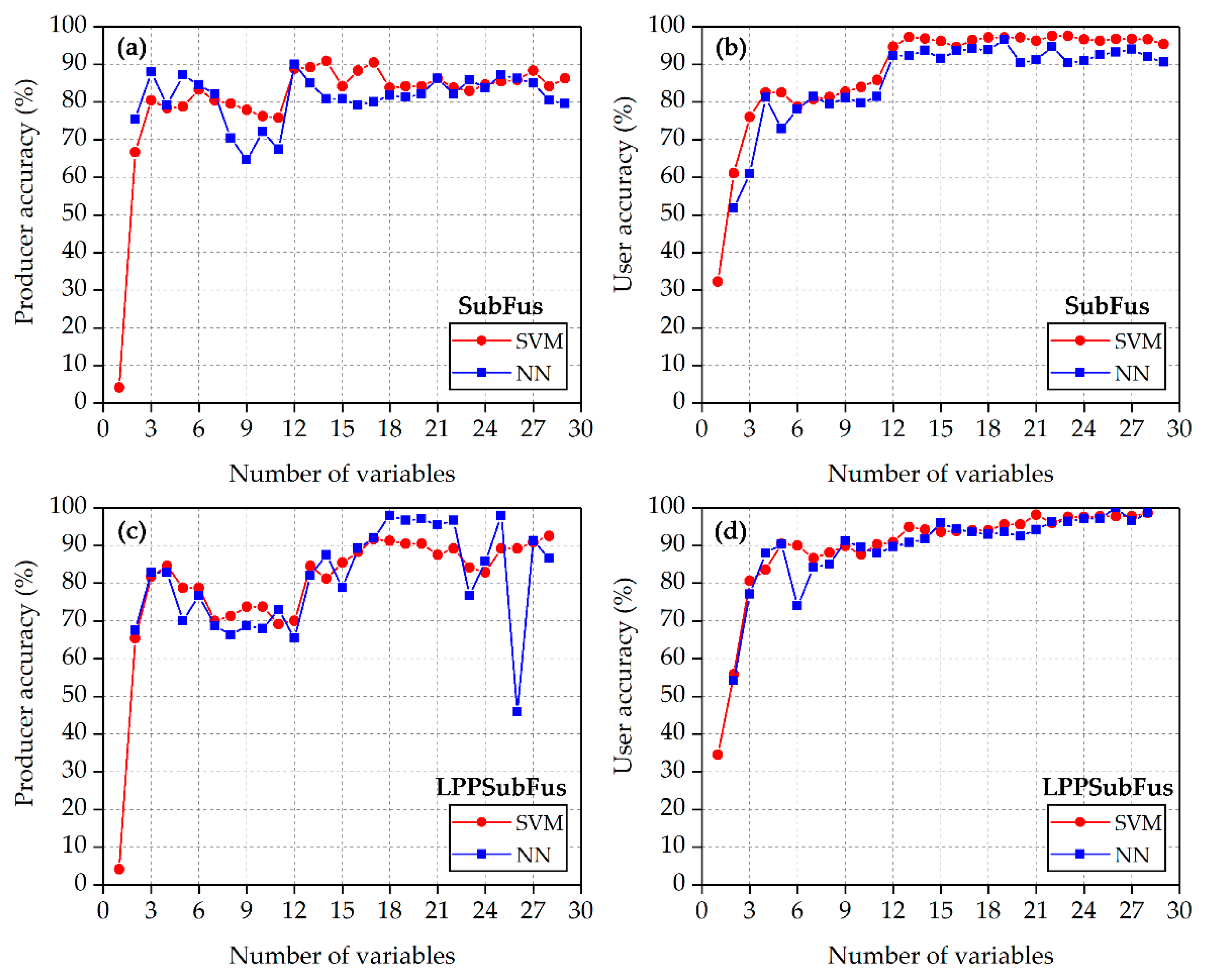
3.2.2. Comparison of Producer and User Accuracy
4. Discussion
4.1. Improvement under Different Fusion Strategies
4.1.1. Comparison of Pixel- and Feature-Level Image Fusion
4.1.2. Comparison of SubFus and LPPSubFus
4.2. Benefits of Image Fusion for Tea Plantation Mapping
4.3. Classification Algorithm for Tea Plantation Mapping
5. Conclusions
- (1)
- FLIF can reduce data dimensionality and significantly improve noise phenomenon and classification accuracy. However, PLIF did not contribute to classification accuracy and even led to decreased accuracy in some cases.
- (2)
- LPPSubFus improved OA by 3% compared to SubFus. In particular, LPPSubFus with NN algorithms achieved the highest OA of 95%, and the PA and UA for tea plantations and forests exceeded 90%, which was concluded to be the best method for tea plantation mapping in this study.
- (3)
- LPPSubFus is compatible with different classification algorithms and had more stable and superior tea plantation mapping performance than PLIF and SubFus.
Author Contributions
Funding
Acknowledgments
Conflicts of Interest
References
- Li, X.; He, Y. Discriminating varieties of tea plant based on Vis/NIR spectral characteristics and using artificial neural networks. Biosyst. Eng. 2008, 99, 313–321. [Google Scholar] [CrossRef]
- Kumar, A.; Manjunath, K.R.; Meenakshi; Bala, R.; Suda, R.K.; Singh, R.D.; Panigrahy, S. Field hyperspectral data analysis for discriminating spectral behavior of tea plantations under various management practices. Int. J. Appl. Earth Obs. Geoinf. 2013, 23, 352–359. [Google Scholar] [CrossRef]
- Wang, Y.; Hao, X.; Wang, L.; Xiao, B.; Wang, X.; Yang, Y. Diverse Colletotrichum species cause anthracnose of tea plants (Camellia sinensis (L.) O. Kuntze) in China. Sci. Rep. 2016, 6, 35287. [Google Scholar] [CrossRef] [PubMed] [Green Version]
- Li, N.; Zhang, D.; Li, L.; Zhang, Y. Mapping the spatial distribution of tea plantations using high-spatiotemporal-resolution imagery in northern Zhejiang, China. Forests 2019, 10, 856. [Google Scholar] [CrossRef] [Green Version]
- FAOSTAT Home Page. Available online: http://www.fao.org/home/en/ (accessed on 28 November 2020).
- Zhang, Z. Shucheng tea plantation optimal ecological zoning based on GIS spatial soil properties. In Proceedings of the 2017 32nd Youth Academic Annual Conference of Chinese Association of Automation, YAC 2017, Hefei, China, 19–21 May 2017; pp. 40–45. [Google Scholar] [CrossRef]
- Akar, Ö.; Güngör, O. Integrating multiple texture methods and NDVI to the Random Forest classification algorithm to detect tea and hazelnut plantation areas in northeast Turkey. Int. J. Remote Sens. 2015, 36, 442–464. [Google Scholar] [CrossRef]
- Chu, H.-J.; Wang, C.-K.; Kong, S.-J.; Chen, K.-C. Integration of full-waveform LiDAR and hyperspectral data to enhance tea and areca classification. GISci. Remote Sens. 2016, 53, 542–559. [Google Scholar] [CrossRef]
- Xu, W.; Qin, Y.; Xiao, X.; Di, G.; Doughty, R.B.; Zhou, Y.; Zou, Z.; Kong, L.; Niu, Q.; Kou, W. Quantifying spatial-temporal changes of tea plantations in complex landscapes through integrative analyses of optical and microwave imagery. Int. J. Appl. Earth Obs. Geoinf. 2018, 73, 697–711. [Google Scholar] [CrossRef]
- Evans, T.L.; Costa, M. Landcover classification of the Lower Nhecolândia subregion of the Brazilian Pantanal Wetlands using ALOS/PALSAR, RADARSAT-2 and ENVISAT/ASAR imagery. Remote Sens. Environ. 2013, 128, 118–137. [Google Scholar] [CrossRef]
- Costa, M.P.F. Use of SAR satellites for mapping zonation of vegetation communities in the Amazon floodplain. Int. J. Remote Sens. 2004, 25, 1817–1835. [Google Scholar] [CrossRef]
- Zhao, D.; Pang, Y.; Liu, L.; Li, Z. Individual tree classification using airborne lidar and hyperspectral data in a natural mixed forest of northeast China. Forests 2020, 11, 303. [Google Scholar] [CrossRef] [Green Version]
- Shang, X.; Chisholm, L.A. Classification of Australian native forest species using hyperspectral remote sensing and machine-learning classification algorithms. IEEE J. Sel. Top. Appl. Earth Obs. Remote Sens. 2014, 7, 2481–2489. [Google Scholar] [CrossRef]
- Hu, J.; Ghamisi, P.; Schmitt, A.; Zhu, X.X. Object based fusion of polarimetric SAR and hyperspectral imaging for land use classification. Work. Hyperspectr. Image Signal Process. Evol. Remote Sens. 2016, 1–5. [Google Scholar] [CrossRef]
- Jouan, A.; Allard, Y. Land use mapping with evidential fusion of polarimetric synthetic aperture Radar and hyperspectral imagery. Inf. Fusion 2002, 5, 251–267. [Google Scholar] [CrossRef]
- Pohl, C.; van Genderen, J. Multisensor image fusion in remote sensing: Concepts, methods and applications. Int. J. Remote Sens. 1998, 19, 823–854. [Google Scholar] [CrossRef] [Green Version]
- Klein, L.A. Sensor and Data Fusion Concepts and Applications, 2nd ed.; Society of Photo-Optical Instrumentation Engineers (SPIE): Bellingham, WA, USA, 1999; ISBN 0819432318. [Google Scholar]
- Wu, Y.; Zhang, X. Object-Based tree species classification using airborne hyperspectral images and LiDAR data. Forests 2020, 11, 32. [Google Scholar] [CrossRef] [Green Version]
- Xi, Y.; Ren, C.; Wang, Z.; Wei, S.; Bai, J.; Zhang, B.; Xiang, H.; Chen, L. Mapping tree species composition using OHS-1 hyperspectral data and deep learning algorithms in Changbai mountains, Northeast China. Forests 2019, 10, 818. [Google Scholar] [CrossRef] [Green Version]
- Shi, Y.; Skidmore, A.K.; Wang, T.; Holzwarth, S.; Heiden, U.; Pinnel, N.; Zhu, X.; Heurich, M. Tree species classification using plant functional traits from LiDAR and hyperspectral data. Int. J. Appl. Earth Obs. Geoinf. 2018, 73, 207–219. [Google Scholar] [CrossRef]
- Fu, B.; Wang, Y.; Campbell, A.; Li, Y.; Zhang, B.; Yin, S.; Xing, Z.; Jin, X. Comparison of object-based and pixel-based Random Forest algorithm for wetland vegetation mapping using high spatial resolution GF-1 and SAR data. Ecol. Indic. 2017, 73, 105–117. [Google Scholar] [CrossRef]
- Wang, X.Y.; Guo, Y.G.; He, J.; Du, L.T. Fusion of HJ1B and ALOS PALSAR data for land cover classification using machine learning methods. Int. J. Appl. Earth Obs. Geoinf. 2016, 52, 192–203. [Google Scholar] [CrossRef]
- Richard, J.; Blaschke, T.; Collins, M. Fusion of TerraSAR-x and Landsat ETM + data for protected area mapping in Uganda. Int. J. Appl. Earth Obs. Geoinf. 2015, 38, 99–104. [Google Scholar] [CrossRef]
- Zhang, H.; Xu, R. Exploring the optimal integration levels between SAR and optical data for better urban land cover mapping in the Pearl River Delta. Int. J. Appl. Earth Obs. Geoinf. 2018, 64, 87–95. [Google Scholar] [CrossRef]
- Kulkarni, S.C.; Rege, P.P. Pixel level fusion techniques for SAR and optical images: A review. Inf. Fusion 2020, 59, 13–29. [Google Scholar] [CrossRef]
- Hu, Q.; Sulla-menashe, D.; Xu, B.; Yin, H.; Tang, H.; Yang, P. A phenology-based spectral and temporal feature selection method for crop mapping from satellite time series. Int. J. Appl. Earth Obs. Geoinf. 2019, 80, 218–229. [Google Scholar] [CrossRef]
- Rasti, B.; Ghamisi, P. Remote sensing image classification using subspace sensor fusion. Inf. Fusion 2020, 64, 121–130. [Google Scholar] [CrossRef]
- Teillet, P.M.; Guindon, B.; Goodenough, D.G. On the slope-aspect correction of multispectral scanner data Seventh International Symposium Machine Processing of remotely sensed data. Can. J. Remote Sens. 1982, 8, 84–106. [Google Scholar] [CrossRef] [Green Version]
- Fraser, R.H.; Olthof, I.; Pouliot, D. Monitoring land cover change and ecological integrity in Canada’s national parks. Remote Sens. Environ. 2009, 113, 1397–1409. [Google Scholar] [CrossRef]
- Asante-Okyere, S.; Shen, C.; Ziggah, Y.Y.; Rulegeya, M.M.; Zhu, X. Principal component analysis (PCA) based hybrid models for the accurate estimation of reservoir water saturation. Comput. Geosci. 2020, 145, 104555. [Google Scholar] [CrossRef]
- Gitelson, A.A.; Gritz, Y.; Merzlyak, M.N. Relationships between leaf chlorophyll content and spectral reflectance and algorithms for non-destructive chlorophyll assessment in higher plant leaves. J. Plant Physiol. 2003, 160, 271–282. [Google Scholar] [CrossRef]
- Gitelson, A.A.; Merzlyak, M.N.; Chivkunova, O.B. Optical properties and nondestructive estimation of anthocyanin content in plant leaves. Photochem. Photobiol. 2001, 74, 38–45. [Google Scholar] [CrossRef]
- Vogelmann, J.E.; Rock, B.N.; Moss, D.M. Red edge spectral measurements from sugar maple leaves. Int. J. Remote Sens. 1993, 14, 1563–1575. [Google Scholar] [CrossRef]
- Kim, Y.; Glenn, D.M.; Park, J.; Ngugi, H.K.; Lehman, B.L. Hyperspectral image analysis for water stress detection of apple trees. Comput. Electron. Agric. 2011, 77, 155–160. [Google Scholar] [CrossRef]
- Negri, R.G.; Dutra, L.V.; Freitas, C.D.C.; Lu, D. Exploring the capability of ALOS PALSAR L-band fully polarimetric data for land cover classification in tropical environments. IEEE J. Sel. Top. Appl. Earth Obs. Remote Sens. 2016, 9, 5369–5384. [Google Scholar] [CrossRef]
- Naidoo, L.; Mathieu, R.; Main, R.; Wessels, K.; Asner, G.P. L-band Synthetic Aperture Radar imagery performs better than optical datasets at retrieving woody fractional cover in deciduous, dry savannahs. Int. J. Appl. Earth Obs. Geoinf. 2016, 52, 54–64. [Google Scholar] [CrossRef]
- Li, G.; Lu, D.; Moran, E.; Dutra, L.; Batistella, M. A comparative analysis of ALOS PALSAR L-band and RADARSAT-2 C-band data for land-cover classification in a tropical moist region. ISPRS J. Photogramm. Remote Sens. 2012, 70, 26–38. [Google Scholar] [CrossRef] [Green Version]
- Moreira, A.; Prats-Iraola, P.; Younis, M.; Krieger, G.; Hajnsek, I.; Papathanassiou, K.P. A tutorial on synthetic aperture radar. IEEE Geosci. Remote Sens. Mag. 2013, 1, 6–43. [Google Scholar] [CrossRef] [Green Version]
- Schmitt, A.; Wendleder, A.; Hinz, S. The Kennaugh element framework for multi-scale, multi-polarized, multi-temporal and multi-frequency SAR image preparation. ISPRS J. Photogramm. Remote Sens. 2015, 102, 122–139. [Google Scholar] [CrossRef] [Green Version]
- Haralick, R.M.; Dinstein, I.; Shanmugam, K. Textural features for image classification. IEEE Trans. Syst. Man Cybern. 1973, SMC-3, 610–621. [Google Scholar] [CrossRef] [Green Version]
- He, X.; Niyogi, P. Locality Preserving Projections; MIT Press: Cambridge, MA, USA, 2004; ISBN 0262201526. [Google Scholar]
- Hu, J.; Hong, D.; Wang, Y.; Zhu, X. A comparative review of manifold learning techniques for hyperspectral and polarimetric SAR image fusion. Remote Sens. 2019, 11, 681. [Google Scholar] [CrossRef] [Green Version]
- Peng, Y.; Wang, Z.; He, K.; Liu, Y.; Li, Q.; Liu, L.; Zhu, X.; Haajek, P. Feature Extraction of Double Pulse Metal Inert Gas Welding Based on Broadband Mode Decomposition and Locality Preserving Projection. Math. Probl. Eng. 2020, 2020, 7576034. [Google Scholar] [CrossRef]
- Evans, D.L.; Farr, T.G.; Ford, J.P.; Thompson, T.W.; Werner, C.L. Multipolarization radar images for geologic mapping and vegetation discrimination. IEEE Trans. Geosci. Remote Sens. 1986, GE-24, 246–257. [Google Scholar] [CrossRef]
- Baghdadi, N.; Bernier, M.; Gauthier, R.; Neeson, I. Evaluation of C-band SAR data for wetlands mapping. Int. J. Remote Sens. 2001, 22, 71–88. [Google Scholar] [CrossRef]
- Duro, D.C.; Franklin, S.E.; Dubé, M.G. A comparison of pixel-based and object-based image analysis with selected machine learning algorithms for the classification of agricultural landscapes using SPOT-5 HRG imagery. Remote Sens. Environ. 2012, 118, 259–272. [Google Scholar] [CrossRef]
- Cai, Y.; Guan, K.; Peng, J.; Wang, S.; Seifert, C.; Wardlow, B.; Li, Z. A high-performance and in-season classification system of field-level crop types using time-series Landsat data and a machine learning approach. Remote Sens. Environ. 2018, 210, 35–47. [Google Scholar] [CrossRef]
- Shao, Y.; Lunetta, R.S. Comparison of support vector machine, neural network, and CART algorithms for the land-cover classification using limited training data points. ISPRS J. Photogramm. Remote Sens. 2012, 70, 78–87. [Google Scholar] [CrossRef]
- Couellan, N.; Wang, W. Bi-level stochastic gradient for large scale support vector machine. Neurocomputing 2015, 153, 300–308. [Google Scholar] [CrossRef]
- Mountrakis, G.; Im, J.; Ogole, C. Support vector machines in remote sensing: A review. ISPRS J. Photogramm. Remote Sens. 2011, 66, 247–259. [Google Scholar] [CrossRef]
- Dihkan, M.; Guneroglu, N.; Karsli, F.; Guneroglu, A. Remote sensing of tea plantations using an SVM classifier and pattern-based accuracy assessment technique. Int. J. Remote Sens. 2013, 34, 8549–8565. [Google Scholar] [CrossRef]
- Melgani, F.; Bruzzone, L. Classification of hyperspectral remote sensing images with support vector machines. IEEE Trans. Geosci. Remote Sens. 2004, 42, 1778–1790. [Google Scholar] [CrossRef] [Green Version]
- Kimes, D.S.; Nelson, R.F.; Manry, M.T.; Fung, A.K. Review article: Attributes of neural networks for extracting continuous vegetation variables from optical and radar measurements. Int. J. Remote Sens. 1998, 19, 2639–2663. [Google Scholar] [CrossRef]
- Xie, Z.; Chen, Y.; Lu, D.; Li, G. Classification of Land Cover, Forest, and Tree Species Classes with ZiYuan-3 Multispectral and Stereo Data. Remote Sens. 2019, 11, 164. [Google Scholar] [CrossRef] [Green Version]
- Paola, J.D.; Schowengerdt, R.A. A Detailed Comparison of Backpropagation Neural Network and Maximum-Likelihood Classifiers for Urban Land Use Classification. IEEE Trans. Geosci. Remote Sens. 1995, 33, 981–996. [Google Scholar] [CrossRef]
- Zhang, C.; Xie, Z. Combining object-based texture measures with a neural network for vegetation mapping in the Everglades from hyperspectral imagery. Remote Sens. Environ. 2012, 124, 310–320. [Google Scholar] [CrossRef]
- Hsu, C.; Chang, C.; Lin, C. A practical guide to support vector classification. BJU Int. 2008, 101, 1396–1400. [Google Scholar]
- Zhu, C.; Luo, J.; Shen, Z.; Huang, C. Wetland mapping in the Balqash lake basin using multi-source remote sensing data and topographic features synergic retrieval. Procedia Environ. Sci. 2011, 10, 2718–2724. [Google Scholar] [CrossRef] [Green Version]
- Zhou, Y.; Hu, J.; Li, Z.; Li, J.; Zhao, R.; Ding, X. Quantifying glacier mass change and its contribution to lake growths in central Kunlun during 2000–2015 from multi-source remote sensing data. J. Hydrol. 2019, 570, 38–50. [Google Scholar] [CrossRef]
- Zhan, T.; Gong, M.; Liu, J.; Zhang, P. Iterative feature mapping network for detecting multiple changes in multi-source remote sensing images. ISPRS J. Photogramm. Remote Sens. 2018, 146, 38–51. [Google Scholar] [CrossRef]
- He, Y.; Chen, G.; Potter, C.; Meentemeyer, R.K. Integrating multi-sensor remote sensing and species distribution modeling to map the spread of emerging forest disease and tree mortality. Remote Sens. Environ. 2019, 231, 111238. [Google Scholar] [CrossRef]
- Yusoff, N.M.; Muharam, F.M.; Takeuchi, W.; Darmawan, S.; Razak, M.H.A. Phenology and classification of abandoned agricultural land based on ALOS-1 and 2 PALSAR multi-temporal measurements. Int. J. Digit. Earth 2017, 10, 155–174. [Google Scholar] [CrossRef]
- Yu, L.; Porwal, A.; Holden, E.J.; Dentith, M.C. Towards automatic lithological classification from remote sensing data using support vector machines. Comput. Geosci. 2012, 45, 229–239. [Google Scholar] [CrossRef]


| Optical Image | SAR Image | |||
|---|---|---|---|---|
| Sensor | Gaofen-5 | Sensor | Sentinel-1A | |
| Spatial resolution | 30 m | Spatial resolution | 5 m × 20 m | |
| Spectral resolution | 5–10 nm | Wavelength | C | |
| Band information | Visible–near-infrared | 0.39–1.03 μm, 150 bands in total | Polarization | VV and VH |
| Short wave infrared | 1.0–2.5 μm, 180 bands in total | |||
| Acquisition time | 19 November 2019 | 18 November 2019 | ||
| Name of Variable | Description |
|---|---|
| Chlorophyll Index 2 | |
| Anthocyanin Reflectance Index 2 | |
| Vogelmann Red Edge Index 2 | |
| Water Band Index |
| Scenario | Image Layer Used for Classification |
|---|---|
| 1 | Optical: first three PC and six bands, seven spectral indexes, and 18 textures. |
| 2 | Optical: first three PC bands, six fusion bands using PCA, seven spectral indexes, and 18 textures; SAR: four polarimetric features, DEM data, and 24 textures. |
| 3 | Optical: first three PC bands, six fusion bands using DWT, seven spectral indexes, and 18 textures; SAR: four polarimetric features, DEM data, and 24 textures. |
| 4 | Optical: first three PC bands, six fusion bands using W-PCA, seven spectral indexes, and 18 textures; SAR: four polarimetric features, DEM data, and 24 textures. |
| 5 | Optical: first three PC and six bands, seven spectral indices, and 18 textures; SAR: four polarimetric features, DEM data, and 24 textures. (SubFus) |
| 6 | Optical: first three PC and six bands of HS data, seven spectral indices, and 18 textures. SAR: four polarimetric features, DEM data, and 24 textures. (LPPSubFus) |
| Sample Type | Training | Test | ||
|---|---|---|---|---|
| Polygons | Pixels | Polygons | Pixels | |
| Tea plantations | 30 | 120 | 60 | 240 |
| Forests | 30 | 120 | 60 | 240 |
| Croplands | 15 | 60 | 30 | 120 |
| Rocks | 15 | 60 | 30 | 120 |
| Built-up area and waterbodies | 15 | 60 | 30 | 120 |
| Total | 105 | 420 | 210 | 840 |
| Scenario | Overall Accuracy | Kappa Coefficient | Classification Algorithm |
|---|---|---|---|
| 1 | 89.05% | 0.8593 | SVM |
| 2 | 89.88% | 0.8698 | |
| 3 | 87.74% | 0.8423 | |
| 4 | 89.40% | 0.8636 | |
| 5 (r = 27) | 89.05% | 0.8589 | |
| 6 (r = 28) | 92.14% | 0.8990 | |
| 1 | 92.14% | 0.8989 | NN |
| 2 | 88.33% | 0.8501 | |
| 3 | 86.07% | 0.8213 | |
| 4 | 87.98% | 0.8458 | |
| 5 (r = 12) | 90.83% | 0.8815 | |
| 6 (r = 22) | 95.00% | 0.9355 |
| Scenario | PA of Tea Plantation (%) | UA of Tea Plantation (%) | PA of Forest (%) | UA of Forest (%) | Classification Algorithm |
|---|---|---|---|---|---|
| 1 | 93.75 | 89.29 | 85.42 | 96.70 | SVM |
| 2 | 94.58 | 89.72 | 86.67 | 95.85 | |
| 3 | 92.92 | 85.11 | 80.83 | 94.17 | |
| 4 | 95.42 | 86.42 | 83.33 | 96.62 | |
| 5 (r = 27) | 93.75 | 87.55 | 88.33 | 96.80 | |
| 6 (r = 28) | 94.58 | 93.80 | 92.50 | 98.67 | |
| 1 | 97.08 | 91.73 | 87.5 | 96.77 | NN |
| 2 | 90.42 | 85.43 | 80.83 | 92.38 | |
| 3 | 90.83 | 83.85 | 76.67 | 92.93 | |
| 4 | 91.67 | 84.94 | 77.92 | 94.92 | |
| 5 (r = 12) | 92.50 | 86.05 | 90.00 | 92.31 | |
| 6 (r = 22) | 96.25 | 94.67 | 96.67 | 96.27 |
Publisher’s Note: MDPI stays neutral with regard to jurisdictional claims in published maps and institutional affiliations. |
© 2020 by the authors. Licensee MDPI, Basel, Switzerland. This article is an open access article distributed under the terms and conditions of the Creative Commons Attribution (CC BY) license (http://creativecommons.org/licenses/by/4.0/).
Share and Cite
Chen, Y.; Tian, S. Feature-Level Fusion between Gaofen-5 and Sentinel-1A Data for Tea Plantation Mapping. Forests 2020, 11, 1357. https://doi.org/10.3390/f11121357
Chen Y, Tian S. Feature-Level Fusion between Gaofen-5 and Sentinel-1A Data for Tea Plantation Mapping. Forests. 2020; 11(12):1357. https://doi.org/10.3390/f11121357
Chicago/Turabian StyleChen, Yujia, and Shufang Tian. 2020. "Feature-Level Fusion between Gaofen-5 and Sentinel-1A Data for Tea Plantation Mapping" Forests 11, no. 12: 1357. https://doi.org/10.3390/f11121357