Article

Development of Crown Ratio and Height to Crown Base Models for Masson Pine in Southern China

1
Research Center of Forest Management Engineering of National Forestry and Grassland Administration, Beijing Forestry University, Beijing 100083, China
2
Academy of Forest Inventory and Planning, National Forestry and Grassland Administration, Beijing 100714, China
*
Author to whom correspondence should be addressed.
Forests 2020, 11(11), 1216; https://doi.org/10.3390/f11111216
Submission received: 26 August 2020 / Revised: 24 October 2020 / Accepted: 16 November 2020 / Published: 19 November 2020
(This article belongs to the Special Issue Modelling and Managing the Dynamics of Pine Forests)

Abstract

:
Crown ratio (CR) and height to crown base (HCB) are important crown characteristics influencing the behavior of forest canopy fires. However, the labor-intensive and costly measurement of CR and HCB have hindered their wide application to forest fire management. Here, we use 301 sample trees collected in 11 provinces in China to produce predictive models of CR and HCB for Masson pine forests (Pinus massoniana Lamb.), which are vulnerable to forest canopy fires. We first identified the best basic model that used only diameter at breast height (DBH) and height (H) as independent variables to predict CR and HCB, respectively, from 11 of the most used potential candidate models. Second, we introduced other covariates into the best basic model of CR and HCB and developed the final CR and HCB predictive models after evaluating the model performance of different combinations of covariates. The results showed that the Richards form of the candidate models performed best in predicting CR and HCB. The final CR model included DBH, H, DBH0.5 and height-to-diameter ratio (HDR), while the final HCB model was the best basic model (i.e., it did not contain any other covariates). We hope that our CR and HCB predictive models contribute to the forest crown fire management of Masson pine forests.

1. Introduction

The tree canopy is an important forest layer where trees interact with their surrounding environment [1,2]. Many key physiological processes related to the growth and development of trees, such as photosynthesis [3,4], respiration [5,6] and transpiration [7,8], occur in the canopy layer. It also plays a vital role in maintaining the soil water of the forest stand [9,10]. Additionally, the tree canopy is the primary fuel stratum involved in independent crown fires [11], and the spatial continuity and density of tree canopies determine the initiation and rate of crown fire spread and severity [12,13]. Therefore, canopy fuel characteristics (e.g., canopy fuel load (CFL), which describes available canopy fuel in the aerial layer [14,15,16]; canopy bulk density (CBD), which indicates the dry weight of the fuel available per canopy volume unity [14,15,16]), have been studied extensively for forest crown fire management [15,17,18]. For instance, CBD has been widely integrated into stand density management diagrams (SDMDs) to guide thinning practices while reducing the potential risk of crown fires [19,20,21]. Many forest growth simulators have incorporated crown characteristics as the explanatory variables in their predictive functions, such as FORMIT-M [22], the Forest Vegetation Simulator (FVS-PROGNOSIS) [23] and the Tree and Stand Simulator (TASS) [24]. Additionally, crown characteristics have also been extensively used as the independent variable for predicting basal area growth [25,26,27,28], as crown characteristics can reflect tree vigor, tree competition status and site quality [29,30,31,32].
Tree crown dimensions are an important feature of the tree canopy. They are generally represented by basic features, such as crown length (CL) and crown width (CW), as well as derivative features, such as the crown ratio (CR) and tree height to crown base (HCB) [33] (Figure S1, in the Supplementary file). CR refers to the ratio of the crown length to the total height of a tree, with values ranging from 0 (for a tree without a crown, such as a dead or defoliated tree) to 1 (for a tree crown that extends over the entire tree trunk) [33]. CR is a robust indicator of photosynthetic capacity [34] and tree stability [35] and provides a means of quantifying tree vitality and stand density [36]. HCB is defined as the height from the ground to the base of the first living branch that is a part of the crown, ranging from 0 to the height of the tree [37], which is usually considered a reflection of the long-term level of competition [38].
Both CR and HCB are important canopy fuel characteristics influencing potential crown fire behavior [14,18,39]. For example, there is a certain relationship between HCB and the occurrence of crown fires: a smaller HCB is associated with a higher potential for surface fires to develop into a crown fire [40,41,42]. Fernandes [43] used CR together with the overstorey height and crown cover of each forest type to calculate wind adjustment factors, which can convert wind speed at the standard 6-m height above the vegetation to the so-called midflame wind speed. The midflame wind speed is a quantification of the canopy-induced decrease in wind speed and can thus represent the within-stand surface wind driving the speed of the fire.
Additionally, CR and HCB have been widely used as predictors of forest growth and in yield models [25,44,45,46,47,48]. For example, Ritchie and Hann [25] and Hann [46] used CR as a predictor to predict individual basal area increment and diameter growth, respectively. Sharma et al. [48] used HCB as an explanatory variable in their crown-to-bole diameter ratio model. Therefore, these metrics are critically important for informing forest fire management, especially for reducing the prevalence of crown fires. However, compared with other tree characteristics, the labor-intensive, time- and money-consuming endeavor of measuring CR and HCB hinders their wide application to forest fire management [36,37]. Consequently, numerous studies have focused on developing predictive models that use common tree variables or easily obtainable stand variables for estimating the CR and HCB of trees. For instance, Fu et al. [33] developed a CR model for Mongolian oak in Northeast China. Rijal et al. [49] produced HCB models for 13 tree species of the North American Acadian Region.
Masson pine (Pinus massoniana Lamb.) is an important tree species in southern China that covers a total area of 10.1 million ha with a stocking of 590 million m3, accounting for 6% of the total area and 4% of the total stocking [50]. The Masson pine forests in China primarily occur in single-species forests, which are unstable and are highly susceptibility to disturbances such as fire, wind and pests [51]. For instance, Masson pine forests experience the highest occurrence rates of wildland fires, resulting in substantial losses of Masson pine forest to fire [52,53,54]. Wu et al. [52] showed that more than 90% of China’s forest fires occur in southern China, mostly in Masson pine forests. Many have found that the susceptibility of forests to crown fire is closely related to CR and HCB [40,55,56]. The crown fire risk can, therefore, be reduced through manipulation of CR and HCB within a reasonable range [57,58,59]. However, there is currently no predictive model for CR and HCB for Masson pine to support prescription of a particular silvicultural regime. Here, we aimed to develop predictive models of CR and HCB using easily measured individual tree variables as predictors. Our predictive models will contribute to the development of a silvicultural strategy that can reduce the potential for forest crown fires.

2. Materials and Methods
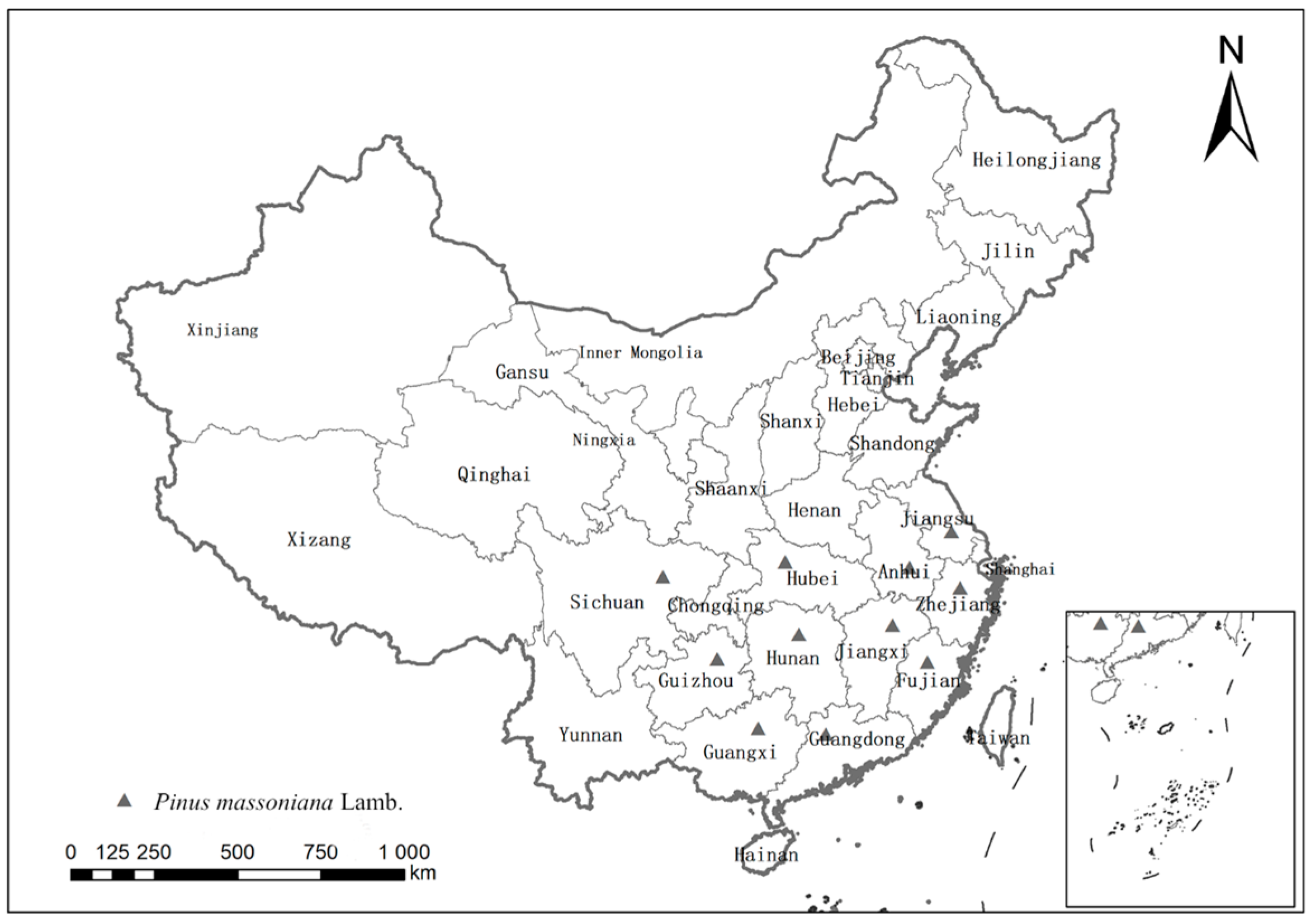
2.1. Data

We used data from the National Biomass Modeling Program in the Continuous Forest Inventory (NBMP-CFI) program funded by the State Forestry Administration of China [60]. These data were collected from 11 provinces in southern China representing the core distribution areas of Masson pine: Anhui, Fujian, Guangdong, Guangxi, Guizhou, Hubei, Hunan, Jiangsu, Jiangxi, Sichuan and Zhejiang (Figure 1). A total of 301 P. massoniana trees were sampled in this study and were evenly distributed among 10 diameter classes (i.e., 2, 4, 6, 8, 12, 16, 20, 26, 32 cm and >38 cm) with about 30 sample trees per diameter class. After measuring the diameter at breast height (DBH) and CW of each sample in the field, the trees were felled, and tree height (H) and CL were measured. The CR and HCB of P. massoniana were calculated based on their definitions. All 301 trees were used for model fitting and validation. Distributions of the measured and derived variables for the 301 trees are shown in Figure 2.

2.2. Model Development

2.2.1. Basic Model Selection

We modeled CR and HCB using logistic, exponential, Richards and Weibull equations [33,37,49,61]. The Richards and Weibull equations are special forms of logistic and exponential equations, respectively [49,61]. We selected six CR models and five HCB models as candidate models (Table 1). Because H and DBH are key predictor variables in modeling forest crown characteristics [37], we used both H and DBH as initial predictor variables in each HCB and CR candidate model. Based on model evaluation and validation, the best basic model was then finally identified for further analysis.

2.2.2. Additional Variable Selection

Stand development stage, site quality, stand density or competition may substantially influence the tree crown [36,48,67]. Hasenauer and Monserud [36] divided the variables that predict CR and HCB into the following three groups: tree size characteristics (SIZE), competition measures (COMP) and site factors (SITE). The β X in candidate models in Table 1 is described as a linear function of the variables of the three groups and is expressed as follows [36,37,61,62]:
β X = β 0 + b × S I Z E + c × C O M P + d × S I T E
where β 0 is the intercept of the model, and b, c and d are a set of parameters of the model.
Size-related attributes included DBH and H. In addition, we also considered transformations of the basic size variables, including the power of DBH (DBH2 and DBH0.5) and the natural logarithm of DBH and H (ln(DBH) and ln(H)). These size-related attributes are important means of describing stand structure, tree vigor and the competitive ability of individual trees, and hence are closely related to CR and HCB [68,69]. For instance, a shorter DBH and a larger tree height, which correspond to a higher stand density, are usually associated with a lower CR (or higher HCB) [37,49].
Competition-related covariates included the height-to-diameter ratio (HDR) and CW. We also considered their transformation, such as the natural logarithm of CW (ln(CW)). HDR has been used extensively to describe tree slenderness, which is significantly associated with the degree of competition within a forest stand [70,71,72]. CW is also a variable that describes competition among neighboring trees and has been used extensively in several studies [73,74,75]. CR generally decreases as HDR or CW increases and vice versa for HCB [62,76].
Site-related covariates were not considered in our study because of a lack of site data. Relative to tree size and competition variables, many authors [36,37] have reported that site variables make insignificant contributions to predictions of CR and HCB.
We selected variables using graphical or visual analysis of the data and examination of the correlation statistics [37,62,63,69,77,78]. Moreover, an analysis of the relationship between the residuals of the original models and the potential regressors (one at a time) was also conducted for variable selection. Different combinations of candidate variables and their transformations were tested in the best base model based on the adjusted determination coefficient ( R a 2 ) and root mean square error (RMSE) [33,78]. Additionally, because many [69,79,80] have suggested that introducing many predictors into models not only impedes computational convergence but also results in biased parameter estimates, we also considered over-parameterization before deciding on the final form of our predictive models.

2.2.3. Parameter Estimation and Evaluation

The parameters of all nonlinear regressions were estimated using the ordinary nonlinear least squares technique [33]. The performance of models was evaluated using four statistical indices: R a 2 , RMSE, Akaike’s information criterion (AIC) and the Bayesian information criterion (BIC) [81,82]. Their formulas are shown below:
R a 2 = 1 ( n 1 n p 1 ) ( i = 1 n ( y i y ^ i ) 2 i = 1 n ( y i y ¯ i ) 2 )
R M S E = i = 1 n ( y i y ^ i ) 2 n p
A I C = 2 L o g l i k + 2 p
B I C = 2 L o g l i k + p l n ( n )
where y i is the observed value, y ^ i is the estimated value, y ¯ i is the mean observed value, n is the number of observations and p is the number of estimated parameters of the model (including the intercept). A model with a high R a 2 and low values of the other indicators (RMSE, AIC and BIC) was judged to have a good fit. Additionally, the presence of heteroscedasticity was checked by plotting the studentized residuals against the predicted values, and normal quantile-quantile (Q-Q) plots were used to check for normality of the studentized residuals [83]. If heteroscedasticity was detected, dependent variables were square-root or logarithm transformed to eliminate heteroscedasticity [84].

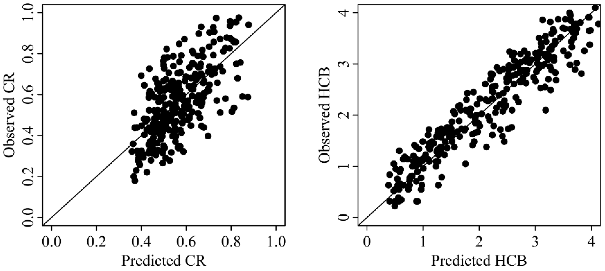
2.3. Model Validation

The robustness and predictive performance of the model was further validated using a 10-fold cross-validation procedure [85,86]. The cross-validation evaluation indicators used in this study included the normalized mean square error for the test set ( N M S E t e ) [87] and the predicted residual error sum of squares (PRESS) [88]. The description of each indicator is as follows:
N M S E t e = I = 1 n ( y I y ^ i ) 2 i = 1 n ( y i y ¯ i ) 2
P R E S S = i = 1 n ( y i y ^ i ) 2
where y i is the observed value, y ^ i is the estimated value and y ^ i is the mean observed value. A model with lower NMSEte and PRESS was judged to have better predictive performance.
All analyses were conducted using R version 3.6.1 statistical software (R Foundation for Statistical Computing, Vienna, Austria) [89]. The following R packages were used in this study: “nlme” [90] for model fitting and “ggplot2” [91] for plotting.

3. Results

3.1. Basic Model Selection

The goodness of fit statistics of model evaluation and validation for all candidate CR models are shown in Table 2. Additionally, we also drew the residual and quantile-quantile (Q-Q) plots of all models and found that they were normally distributed without obvious heteroscedasticity (Figure 3). Furthermore, plots of the predicted values versus the observed values of all models (Figure S2, in the Supplementary file) indicated that there were no differences among these models. Although the CR4 model performed best in model evaluation and validation, the predictive value of CR4 cannot be constrained to [0, 1], meaning that this model lacks biological relevance. After the CR4 model, the CR2 model showed the highest performance and was therefore selected as the best base model to further develop the final CR model. The best basic model form for CR was the following:
C R = 1 / ( 1 + e ( 1.287 + 0.097 × D B H 0.313 × H ) ) 1 6
In the process of selecting the best basic model of HCB, we found that the residuals of all candidate models showed pronounced heteroscedasticity (Figure S3, in the Supplementary file). Additionally, the plots of the predicted values versus the observed values for all HCB candidate models revealed a tendency for overestimation (Figure S4, in the Supplementary file). However, the heteroscedasticity was successfully mitigated (Figure 4) and the tendency of overestimation was ameliorated (Figure S5, in the Supplementary file) by conducting a square-root transformation of the dependent variable.
The goodness of fit statistics of model evaluation and validation for all candidate HCB models with the square-root transformation are shown in Table 3. Although there were almost no significant differences in the performance of all HCB candidate models, HCB2 and HCB4 were slightly better performing than the other models. The model HCB4 was not considered, given that the range of dependent variables could not be limited to [0, H]. Therefore, we selected the HCB2 model as the best basic model form to construct the final model of HCB. The best basic model for predicting HCB was the following:
H C B = H / ( 1 + e ( 8.441 + 0.084 × D B H ) ) 1 6

3.2. Inclusion of Additional Covariates

The relationships among the dependent variables (CR and HCB), the candidate covariates and their transformation were first investigated by performing a visual analysis (Figures S6 and S7, in the Supplementary file). We found that all of the candidate covariates and their transformations were negatively correlated with CR (Figure S6). In contrast, HCB showed a positive relationship with all of the candidate covariates and their transformation, except for HDR, which exhibited a negative correlation (Figure S7). Furthermore, we also conducted a Pearson correlation analysis to quantitively investigate the relationships among the dependent variables (CR and HCB), the candidate covariates and their transformation. The correlation coefficients are shown in Table 4. We found that the results of the Pearson correlation analysis were consistent with the visual analysis.
To identify additional covariates, we also performed an analysis of the relationship between the residuals of the original basic models and the potential regressors (one at a time) (Figures S8 and S9, in the Supplementary file). We found that almost all of the residuals improved after adding the regressors (one at a time). Similar to Temesgen et al. [62], the inclusion of HDR in the best basic model of CR improved the performance of the model, although the correlation between HDR and CR was not significant in this study (Table 4). Thus, we still considered HDR when developing the final CR model.
Based on the best basic model, different combinations of additional covariates were added and examined. We identified the best combination of additional covariates for the best basic model of CR and HCB (Table 5) based on adjusted determination coefficients and root mean square error. In general, we observed that the performance of the model improved as additional covariates were added (Table 6). For instance, the R a 2 increased by 0.058 from 0.3983 (initial variables: DBH and H) to 0.4563 (two additional covariates: DBH0.5 and HDR). However, the R a 2 only increased by 0.0089 from 0.4563 (two additional covariates: DBH0.5 and HDR) to 0.4652 (three additional covariates: DBH2, DBH0.5, HDR). Consequently, in order to maximize model simplicity and generality, we finally selected CR2_1 as our final CR predictive model, which was written as follows:
C R = 1 / ( 1 + e ( 5.217 + 0.274 × D B H 0.097 × H 2.603 × D B H 0.5 2.504 × H D R ) ) 1 6
The residual plot and quantile-quantile (Q-Q) plot of the final CR model is shown in Figure 5. The residuals were normally distributed with no pronounced heteroscedasticity.
For the best basic HCB model (HCB2), the best combination of additional covariates is shown in Table 5. The models improved slightly when covariates were added (Table 7). However, since CW measurement in these models is labor-intensive as well as time- and money-consuming, we decided to not introduce any additional covariates and selected the best basic HCB model (HCB2) as our final HCB model. Figure 6 shows the comparison between the predicted and observed values of the final CR and HCB models.

4. Discussion

To systematically compare this research with existing models, we constructed a table for other similar models containing model equations, tree species, predictors and lack of fit statistics (i.e., R 2 or RMSE) (Table S1, in the Supplementary file). The equations for predicting CR and HCB are mainly logistic equations, followed by exponential equations (Table S1). The final CR and HCB models of Masson pine in this study were developed based on the best candidate model (basic model): the Richards equation (a special form of the logistic equation). The advantage of this form is that the prediction of CR and HCB can be constrained to be between 0 and 1 as well as between 0 and H, which avoids the generation of predictions that are inconsistent with reality [33,36]. Furthermore, the Richards form has also been found to significantly reduce biases, and the problems of convergence rarely occur [49]. Thus, the Richards form has been used extensively to model crown characteristics, such as CR [61,63], HCB [49,66] and CW [78]. However, the best candidate model (basic model) might change after additional covariates are included.
Similar to other CR and HCB modeling studies (Table S1), DBH and H were also the key predictors for predicting CR and HCB in our study. This could be because H and DBH can describe tree structure, tree vigor and competitive ability well [37,69]. Additionally, we also included potential covariates into the best basic model for CR and HCB. Generally, we found that the model performance of CR and HCB improved with the addition of covariates. However, improvements in performance with the addition of covariates were minor for the HCB model; therefore, the best basic model of HCB was selected as our final HCB model.
In contrast, there was a pronounced improvement in the performance of the CR model when other covariates were introduced. In addition to DBH and H, HDR and DBH0.5 were included in our final CR model. Many authors [36,62,63,64] have shown that HDR is a robust predictor of CR and some of them [36,64] have argued that HDR can be considered as an indicator of past competition. For instance, Dyer and Burkhart [64] found that HDR made significant contributions to predicting CR and they think this ability to predict CR stems from the fact that HDR largely accounted for the effect of density on CR; that is, HDR can accurately represent local competition status. Therefore, HDR can serve as a good surrogate for local competition in the absence of competition variables.
Generally, a tree with a greater diameter or a smaller tree height is associated with a higher CR (or lower HCB) in a stand [33,49]. The findings of our study are consistent with this conclusion. In general, the canopy of a larger tree that grows better in a stand experiences less competition from surrounding trees and has better light conditions, resulting in higher crown length (or lower HCB) [81]. Additionally, we observed that CR was negatively correlated with tree height while HCB was positively correlated with tree height. This observation suggested that taller trees in a dense stand experience a greater degree of competition and physical interactions from neighboring trees, or poorer light conditions under the canopy of taller trees, which may result in crown recession and a larger HCB (or lower CR). We also observed that CR was negatively correlated with HDR. This same finding has been reported by several other studies [49,61,62,69]. HDR has also been called the slenderness coefficient, as it is usually associated with a tree’s mechanical stability when calculated at the level of the individual tree [92]. Therefore, HDR has been used extensively to characterize stand stability against disturbances, such as wind and snow [20,72,92].
Many authors have established models of CR and HCB for different tree species (Table S1). The coefficient of determination ( R 2 ) and RMSE have often been used to measure model performance. For CR models, the values of R 2 and RMSE are mainly in the range of 0.09–0.94 and 0.041–0.168, respectively; in contrast, the range of R2 and RMSE for HCB models is 0.04–0.91 and 0.239–3.330, respectively. In our study, the value of R a 2 and RMSE in the CR model was 0.46 and 0.128. These values were within the range of previous studies, suggesting that our CR model is applicable for Masson pine forests in China with an appropriate level of reliability. In comparison, the value of RMSE was 0.350 and R a 2 was 0.88 in our HCB model, which is better than most of those documented in previous studies. However, our HCB model only contained DBH and H relative to existing models. The distinguished performance of our HCB model might be explained by the stable (linear) relationship between H and HCB, which also explains why there was little difference among model candidates of HCB. In contrast, the other independent variable (CW) was measured before the trees were felled. Moreover, it was generally more difficult to measure CW, which may have resulted in less accurate measurements.
Competition indices are frequently used as predictors in CR and HCB models (Table S1). For instance, Hasenauer and Monserud [36] included crown competition factor (CCF) in their CR model for Austrian forests. Sharma et al. [69] introduced basal area in larger trees (BAL) to predict HCB. In addition, many [63,69,93] have insisted that including site-related covariates, such as elevation, site index, slope and aspect, could significantly improve model performance; however, some [36,49,62] have disagreed with this suggestion and have argued that these variables only contribute 1% to 5% to the R2 in CR and HCB models.
Mixed-effect models have been extensively used to develop forestry models, such as the individual tree diameter growth model [77,94,95,96,97], the tree crown width model [78,80,98,99], the site index model [100,101,102] and the biomass model [103,104,105,106]. These studies have shown that mixed-effect models can significantly improve model performance. For instance, Fu et al. [33] reported that the R2 increased from 0.26 to 0.64 after introducing both blocks and the interaction of blocks and sample plots as random effects when developing a crown ratio model. Pokharel and Dech [107] included ecological land classification (ELC) ecosites as a random effect to predict basal area growth and found that the model’s performance was also significantly improved. They attributed the improvement to the fact that ELC ecosites used substrate characteristics (e.g., soil texture, moisture regime and soil depth) and overstorey tree species composition to delineate forest conditions. Therefore, ELC could accurately represent the specific site environment of each tree.
In our study, detailed site information, such as ELC ecosites, were not available; we only had access to information on the province in which each tree was located. Including province as a random effect in the models did not improve model performance, which might stem from the fact that the delimitation of provinces is not inherently based on the biological, geographical and climatic factors that significantly affect tree growth. In future studies, site conditions and other types of relevant information affecting the environments associated with trees need to be collected when conducting forest inventories.

5. Conclusions

Here, we developed CR and HCB models for Masson pine in southern China. In practice, forest managers could use our CR and HCB models combined with other forest models (e.g., the basal area increment model and crown width model) to estimate crown surface area, crown volume and crown biomass. Additionally, CR and HCB models can also be used as submodels in forest growth simulators, which are useful tools for prescribing forest management strategies. Most importantly, CR and HCB are critically important for forest fire management, as these models can be used in fire modeling systems that can be used to assess crown fire hazards and provide fuel treatment alternatives for forest managers. However, other canopy fuel characteristics, such as CFL and CBD, were not examined because of a lack of data. We encourage future studies to examine these other canopy fuel characteristics, given that the joint consideration of all possible fuel characteristics would facilitate the development of forest fire management strategies.

Supplementary Materials

The following are available online at https://www.mdpi.com/1999-4907/11/11/1216/s1. Table S1. Detail information of crown ratio and height to crown base mode in existing literature; Figure S1. Schematic diagram of tree crown dimensions; Figure S2. Plots of predicted values against observed values of CR candidate models; Figure S3. Residual and quantile-quantile (Q-Q) plots of HCB candidate models. The solid lines in residual plots is a smoothing spline; Figure S4. Plots of predicted values against observed values of HCB candidate models; Figure S5. Plots of predicted values against observed values of HCB candidate models with root square-transformed data; Figure S6. Scatter plot of CR and all variables; Figure S7. Scatter plot of HCB and all variables; Figure S8. Residuals of the CR best base model with the potential covariates. The first subplot showed the residual of the CR best base model; Figure S9. Residuals of the HCB best base model with the potential covariates. The first subplot showed the residual of the HCB best base model.

Author Contributions

J.M. and W.Z. conceived, designed and performed the experiments; Y.L. analyzed the data and results; W.W., W.Z. and J.W. contributed materials/analysis tools; J.M. and Y.L. are the main authors who developed and revised the manuscript. All authors have read and agreed to the published version of the manuscript.

Funding

This research was funded by the National Key R&D Program of China, Grant Number 2017YFC0505604.

Acknowledgments

We thank the Academy of Forest Inventory and Planning, National Forestry and Grassland Administration, China, which provided support for data access during our research.

Conflicts of Interest

The authors declare no conflict of interest.

References

  1. Muth, C.C.; Bazzaz, F.A. Tree canopy displacement and neighborhood interactions. Can. J. For. Res. 2003, 33, 1323–1330. [Google Scholar] [CrossRef]
  2. Carreiras, J.M.B.; Pereira, J.M.C.; Pereira, J.S. Estimation of tree canopy cover in evergreen oak woodlands using remote sensing. For. Ecol. Manag. 2006, 223, 45–53. [Google Scholar] [CrossRef]
  3. Terashima, I.; Hikosaka, K. Comparative ecophysiology of leaf and canopy photosynthesis. Plant Cell Environ. 1995, 18, 1111–1128. [Google Scholar] [CrossRef]
  4. Ma, S.Y.; Osuna, J.; Verfaillie, J.; Baldocchi, D. Photosynthetic responses to temperature across leaf–canopy–ecosystem scales: A 15-year study in a Californian oak-grass savanna. Photosynth. Res. 2017, 132. [Google Scholar] [CrossRef]
  5. Turnbull, M.H.; Whitehead, D.; Tissue, D.T.; Schuster, W.S.F.; Brown, K.J.; Griffin, K.L. Scaling Foliar Respiration in Two Contrasting Forest Canopies. Funct. Ecol. 2003, 17, 101–114. [Google Scholar] [CrossRef]
  6. Drake, J.; Tjoelker, M.; Aspinwall, M.; Reich, P.; Barton, C.; Medlyn, B.; Duursma, R. Does physiological acclimation to climate warming stabilize the ratio of canopy respiration to photosynthesis? New Phytol. 2016, 211, 850–863. [Google Scholar] [CrossRef]
  7. Schulze, E.D.; Čermák, J.; Matyssek, M.; Penka, M.; Zimmermann, R.; Vasícek, F.; Gries, W.; Kučera, J. Canopy transpiration and water fluxes in the xylem of the trunk of Larix and Picea trees—A comparison of xylem flow, porometer and cuvette measurements. Oecologia 1985, 66, 475–483. [Google Scholar] [CrossRef]
  8. Köstner, B.M.M.; Schulze, E.D.; Kelliher, F.M.; Hollinger, D.Y.; Byers, J.N.; Hunt, J.E.; McSeveny, T.M.; Meserth, R.; Weir, P.L. Transpiration and canopy conductance in a pristine broad-leaved forest of Nothofagus: An analysis of xylem sap flow and eddy correlation measurements. Oecologia 1992, 91, 350–359. [Google Scholar] [CrossRef]
  9. Meinzer, F.C.; Andrade, J.L.; Goldstein, G.; Holbrook, N.M.; Cavelier, J.; Wright, S.J. Partitioning of soil water among canopy trees in a seasonally dry tropical forest. Oecologia 1999, 121, 293–301. [Google Scholar] [CrossRef]
  10. Zhang, X.; Luo, L.; Jing, W.; Wang, S.; Wang, R.; Che, Z. Study on the Distribution Effect of Canopy Interception of Picea Crassifolia Forest in Qilian Mountains. J. Mt. Sci. 2007, 25, 678–683. [Google Scholar] [CrossRef]
  11. Scott, J.H.; Reinhardt, E.D.; Station, R.M.R. Assessing Crown Fire Potential by Linking Models of Surface and Crown Fire Behavior; U.S. Department of Agriculture, Forest Service, Rocky Mountain Research Station: Fort Collins, CO, USA, 2001. [CrossRef] [Green Version]
  12. Peterson, D.L.; Johnson, M.C.; Agee, J.K.; Jain, T.B.; McKenzie, D.; Reinhardt, E.D. Forest Structure and Fire Hazard in Dry Forests of the Western United States; U.S. Department of Agriculture, Forest Service, Pacific Northwest Research Station: Portland, OR, USA, 2005. [CrossRef]
  13. Lentile, L.; Smith, F.; Shepperd, W. Influence of topography and forest structure on patterns of mixed severity fire in ponderosa pine forests of the South Dakota Black Hills, USA. Int. J. Wildland Fire 2006, 15, 557–566. [Google Scholar] [CrossRef]
  14. Cruz, M.; Alexander, M.; WakimotoC, R. Assessing canopy fuel stratum characteristics in crown fire prone fuel types of western North America. Int. J. Wildland Fire 2003, 12. [Google Scholar] [CrossRef] [Green Version]
  15. Fernández-Alonso, J.M.; Alberdi, I.; Álvarez-González, J.G.; Vega, J.A.; Cañellas, I.; Ruiz-González, A.D. Canopy fuel characteristics in relation to crown fire potential in pine stands: Analysis, modelling and classification. Eur. J. For. Res. 2013, 132, 363–377. [Google Scholar] [CrossRef]
  16. Mitsopoulos, I.D.; Dimitrakopoulos, A.P. Estimation of canopy fuel characteristics of Aleppo pine (Pinus halepensis Mill.) forests in Greece based on common stand parameters. Eur. J. For. Res. 2014, 133, 73–79. [Google Scholar] [CrossRef]
  17. Keyes, C.; O’Hara, K. Quantifying Stand Targets for Silvicultural Prevention of Crown Fires. West. J. Appl. For. 2002, 17, 101–109. [Google Scholar] [CrossRef] [Green Version]
  18. Ruiz-González, A.; Álvarez-González, J. Canopy bulk density and canopy base height equations for assessing crown fire hazard in Pinus radiata plantations. Can. J. For. Res. 2011, 41, 839–850. [Google Scholar] [CrossRef]
  19. Sherlock, J.W. Integrating stand density management with fuel reduction. In Restoring Fire-Adapted Ecosystems: Proceedings of the 2005 National Silviculture Workshop; Powers, R.F., Ed.; PSW-GTR-203; Pacific Southwest Research Station, Forest Service, U.S. Department of Agriculture: Albany, CA, USA, 2007; pp. 55–66. [Google Scholar]
  20. López-Sánchez, C.; Rodríguez-Soalleiro, R. A Density Management Diagram Including Stand Stability and Crown Fire Risk for Pseudotsuga Menziesii (Mirb.) Franco in Spain. Mt. Res. Dev. 2009, 29, 169–176. [Google Scholar] [CrossRef]
  21. Gómez-Vázquez, I.; Fernandes, P.; Arias-Rodil, M.; Anta, M.; Castedo-Dorado, F. Using density management diagrams to assess crown fire potential in Pinus pinaster Ait. stands. Ann. For. Sci. 2014, 473–484. [Google Scholar] [CrossRef] [Green Version]
  22. Härkönen, S.; Neumann, M.; Mues, V.; Berninger, F.; Bronisz, K.; Cardellini, G.; Chirici, G.; Hasenauer, H.; Koehl, M.; Lang, M.; et al. A climate-sensitive forest model for assessing impacts of forest management in Europe. Environ. Model. Softw. 2019, 115, 128–143. [Google Scholar] [CrossRef]
  23. Mitchell, K.J. Dynamics and Simulated Yieldof Douglas-fir. For. Sci. 1975, 21, a0001–z0001. [Google Scholar] [CrossRef]
  24. Wykoff, W.; Crookston, N.L.; Stage, A.; Forest, I.; Station, R.E. User’s Guide to the Stand Prognosis Model; U.S. Dept. of Agriculture, Forest Service, Intermountain Forest and Range Experiment Station: Ogden, UT, USA, 1982.
  25. Ritchie, M.; Hann, D. Equations for predicting basal area increment in Douglas-fir and grand fir. Or. State Univ. For. Res. Lab. Res. Bull. 1985, 51. Available online: https://ir.library.oregonstate.edu/downloads/wd375x45s (accessed on 11 November 2020).
  26. Wykoff, W.R. A Basal Area Increment Model for Individual Conifers in the Northern Rocky Mountains. For. Sci. 1990, 36, 1077–1104. [Google Scholar] [CrossRef]
  27. Biging, G.S.; Dobbertin, M. A Comparison of Distance-Dependent Competition Measures for Height and Basal Area Growth of Individual Conifer Trees. For. Sci. 1992, 38, 695–720. [Google Scholar] [CrossRef]
  28. Monserud, R.A.; Sterba, H. A basal area increment model for individual trees growing in even- and uneven-aged forest stands in Austria. For. Ecol. Manag. 1996, 80, 57–80. [Google Scholar] [CrossRef]
  29. Cole, W.G.; Lorimer, C.G. Predicting tree growth from crown variables in managed northern hardwood stands. For. Ecol. Manag. 1994, 67, 159–175. [Google Scholar] [CrossRef]
  30. Zarnoch, S.; Bechtold, W.A.; Stolte, K. Using crown condition variables as indicators of forest health. Can. J. For. Res.-Rev. Can. De Rech. For. Can J For. Res 2004, 34, 1057–1070. [Google Scholar] [CrossRef]
  31. Sharma, R.; Vacek, Z.; Vacek, S. Generalized Nonlinear Mixed-Effects Individual Tree Crown Ratio Models for Norway Spruce and European Beech. Forests 2018, 9, 555. [Google Scholar] [CrossRef] [Green Version]
  32. Cameron, I.; Parish, R.; Goudie, J.; Statland, C. Modelling the Crown Profile of Western Hemlock (Tsuga heterophylla) with a Combination of Component and Aggregate Measures of Crown Size. Forests 2020, 11, 281. [Google Scholar] [CrossRef] [Green Version]
  33. Fu, L.; Zhang, H.; Lu, J.; Zang, H.; Lou, M.; Wang, G.; Wang, L. Multilevel Nonlinear Mixed-Effect Crown Ratio Models for Individual Trees of Mongolian Oak (Quercus mongolica) in Northeast China. PLoS ONE 2015, 10, e0133294. [Google Scholar] [CrossRef]
  34. Leites, L.; Robinson, A.; Crookston, N. Accuracy and equivalence testing of crown ratio models and assessment of their impact on diameter growth and basal area increment predictions of two variants of the Forest Vegetation Simulator. Can. J. For. Res. 2009, 39, 655–665. [Google Scholar] [CrossRef]
  35. Wilson, J.S.; Oliver, C.D. Stability and density management in Douglas-fir plantations. Can. J. For. Res. 2000, 30, 910–920. [Google Scholar] [CrossRef]
  36. Hasenauer, H.; Monserud, R.A. A crown ratio model for Austrian forests. For. Ecol. Manag. 1996, 84, 49–60. [Google Scholar] [CrossRef]
  37. Fu, L.; Zhang, H.; Sharma, R.; Lifeng, P.; Wang, G. A generalized nonlinear mixed-effects height to crown base model for Mongolian oak in northeast China. For. Ecol. Manag. 2016, 384, 34–43. [Google Scholar] [CrossRef]
  38. Petersson, H. Functions for predicting crown height of Pinus sylvestris and Picea abies in Sweden. Scand. J. For. Res. 1997, 12, 179–188. [Google Scholar] [CrossRef]
  39. Jiménez, E.; Vega, J.; Fernández-Alonso, J.; Vega-Nieva, D.; González, J.; Ruiz-González, A. Allometric equations for estimating canopy fuel load and distribution of pole-size maritime pine trees in five Iberian provenances. Can. J. For. Res. 2013, 43, 149. [Google Scholar] [CrossRef]
  40. Wagner, C.E.V. Conditions for the start and spread of crown fire. Can. J. For. Res. 1977, 7, 23–34. [Google Scholar] [CrossRef]
  41. McAlpine, R.S.; Hobbs, M.W. Predicting the height to live crown base in plantations of four boreal forest species. Int. J. Wildland Fire 1994, 4, 103–106. [Google Scholar] [CrossRef]
  42. Butler, B.W.; Finney, M.A.; Andrews, P.L.; Albini, F.A. A radiation-driven model for crown fire spread. Can. J. For. Res. 2004, 34, 1588–1599. [Google Scholar] [CrossRef]
  43. Fernandes, P.M. Combining forest structure data and fuel modelling to classify fire hazard in Portugal. Ann. For. Sci. 2009, 66, 415. [Google Scholar] [CrossRef] [Green Version]
  44. Short Iii, E.A.; Burkhart, H.E. Predicting Crown-Height Increment for Thinned and Unthinned Loblolly Pine Plantations. For. Sci. 1992, 38, 594–610. [Google Scholar] [CrossRef]
  45. Monserud, R.A.; Sterba, H. Modeling individual tree mortality for Austrian forest species. For. Ecol. Manag. 1999, 113, 109–123. [Google Scholar] [CrossRef]
  46. Hann, D.J.O.S.U. ORGANON user’s Manual Edition 8.2 [Computer Manual]; Department of Forest Resources: Corvallis, OR, USA, 2006.
  47. Kuprevicius, A.; Auty, D.; Achim, A.; Caspersen, J.P. Quantifying the influence of live crown ratio on the mechanical properties of clear wood. For. Int. J. For. Res. 2013, 86, 361–369. [Google Scholar] [CrossRef] [Green Version]
  48. Sharma, R.; Vacek, Z.; Vacek, S. Modelling tree crown-to-bole diameter ratio for Norway spruce and European beech. Silva Fenn. 2017, 51, 1740. [Google Scholar] [CrossRef] [Green Version]
  49. Rijal, B.; Weiskittel, A.; Kershaw, J. Development of height to crown base models for thirteen tree species of the North American Acadian Region. For. Chron. 2012, 88, 60–73. [Google Scholar] [CrossRef] [Green Version]
  50. Administration, C.S.F. China Forest Resource Report (2014–2018); China Forestry Press: Beijing, China, 2019. [Google Scholar]
  51. Meng, J.; Lu, Y.; Zeng, J. Transformation of a Degraded Pinus massoniana Plantation into a Mixed-Species Irregular Forest: Impacts on Stand Structure and Growth in Southern China. Forests 2014, 5, 3199–3221. [Google Scholar] [CrossRef]
  52. Wu, D.; Yi, S.; Liu, A.; Liu, S.; Cai, M. Understory Burning In Stands Of Masson’s Pine. Fire Saf. Sci. 2003, 7, 545–556. [Google Scholar] [CrossRef]
  53. Molina, J.R.; Silva, F.R.Y.; Herrera, M.Á. Potential crown fire behavior in Pinus pinea stands following different fuel treatments. For. Syst. 2011, 20, 266–267. [Google Scholar] [CrossRef] [Green Version]
  54. Xue, L.; Li, Q.; Chen, H. Effects of a Wildfire on Selected Physical, Chemical and Biochemical Soil Properties in a Pinus massoniana Forest in South China. Forests 2014, 5, 2947–2966. [Google Scholar] [CrossRef] [Green Version]
  55. Fernandes, P.; Luz, A.L.; Loureiro, C.; Godinho-Ferreira, P.; Botelho, H. Fuel modelling and fire hazard assessment based on data from the Portuguese National Forest Inventory. For. Ecol. Manag. 2006, 234. [Google Scholar] [CrossRef]
  56. Fajvan, M.A. The Role of Silvicultural Thinning in Eastern Forests Threatened by Hemlock Woolly Adelgid (Adelges tsugae). In Proceedings of USDA Forest Service-General Technical Report PNW-GTR; U.S. Department of Agriculture, Forest Service, Pacific Northwest Research Station: Portland, OR, USA, 2007; pp. 247–256. [Google Scholar]
  57. Azuma, D.; Monleon, V.; Gedney, D. Equations for Predicting Uncompacted Crown Ratio Based on Compacted Crown Ratio and Tree Attributes. West. J. Appl. For. 2004, 19, 260–267. [Google Scholar] [CrossRef] [Green Version]
  58. Mitsopoulos, I.D.; Dimitrakopoulos, A.P. Canopy fuel characteristics and potential crown fire behavior in Aleppo pine (Pinus halepensis Mill.) forests. Ann. For. Sci. 2007, 64, 287–299. [Google Scholar] [CrossRef] [Green Version]
  59. Keyser, T.; Smith, F. Influence of Crown Biomass Estimators and Distribution on Canopy Fuel Characteristics in Ponderosa Pine Stands of the Black Hills. For. Sci. 2010, 56, 156–165. [Google Scholar]
  60. Zeng, W. Modeling Crown Biomass for Four Pine Species in China. Forests 2015, 6, 433–449. [Google Scholar] [CrossRef] [Green Version]
  61. Soares, P.; Tomé, M. A tree crown ratio prediction equation for eucalypt plantations. Ann. For. Sci. 2001, 58, 193–202. [Google Scholar] [CrossRef] [Green Version]
  62. Temesgen, H.; LeMay, V.; Mitchell, S.J. Tree crown ratio models for multi-species and multi-layered stands of southeastern British Columbia. For. Chron. 2005, 81, 133–141. [Google Scholar] [CrossRef]
  63. Popoola, F.S.; Adesoye, P. Crown Ratio Models for Tectona grandis (Linn. f) Stands in Osho Forest Reserve, Oyo State, Nigeria. J. For. Sci. 2012, 28, 63–67. [Google Scholar] [CrossRef]
  64. Dyer, M.E.; Burkhart, H.E. Compatible crown ratio and crown height models. Can. J. For. Res. 1987, 17, 572–574. [Google Scholar] [CrossRef]
  65. Walters, D.; Hann, D. Taper equations for six conifer species in southwest Oregon. Or. State Univ. For. Res. Lab. Res. Bull. 1986, 56, 1–41. [Google Scholar]
  66. Duan, G.; Li, X.; Feng, Y.; Fu, L. Generalized nonlinear mixed-effects crown base height model of Larix principis-rupprechtii natural secondary forests. J. Nanjing For. Univ. 2018, 42, 170–176. [Google Scholar] [CrossRef]
  67. Garber, S.M.; Monserud, R.A.; Maguire, D.A. Crown recession patterns in three conifer species of the northern Rocky Mountains. For. Sci. 2008, 54, 633–646. [Google Scholar]
  68. Sumida, A.; Miyaura, T.; Torii, H. Relationships of tree height and diameter at breast height revisited: Analyses of stem growth using 20-year data of an even-aged Chamaecyparis obtusa stand. Tree Physiol. 2013, 33, 106–118. [Google Scholar] [CrossRef] [PubMed]
  69. Sharma, R.; Vacek, Z.; Vacek, S.; Podrázský, V.; Jansa, V. Modelling individual tree height to crown base of Norway spruce (Picea abies (L.) Karst.) and European beech (Fagus sylvatica L.). PLoS ONE 2017, 12, e0186394. [Google Scholar] [CrossRef] [PubMed] [Green Version]
  70. Zumrawi, A.; Hann, D. Equations for predicting the height to crown base of six tree species in the central Willamette Valley of Oregon. Or. State Univ. For. Res. Lab. 1989, 52, 1–9. [Google Scholar]
  71. Wang, Y.; Titus, S.J.; LeMay, V.M. Relationships between tree slenderness coefficients and tree or stand characteristics for major species in boreal mixedwood forests. Can. J. For. Res. 1998, 28, 1171–1183. [Google Scholar] [CrossRef]
  72. Zhang, X.; Wang, H.; Chhin, S.; Zhang, J. Effects of competition, age and climate on tree slenderness of Chinese fir plantations in southern China. For. Ecol. Manag. 2020, 458, 117815. [Google Scholar] [CrossRef]
  73. Kahriman, A.; Şahin, A.; Sonmez, T.; Yavuz, M. A novel approach to selecting a competition index: The effect of competition on individual tree diameter growth of Calabrian pine. Can. J. For. Res. 2018, 48, 1217–1226. [Google Scholar] [CrossRef]
  74. Krajicek, J.E.; Brinkman, K.A.; Gingrich, S.F. Crown Competition-A Measure of Density. For. Sci. 1961, 7, 35–42. [Google Scholar] [CrossRef]
  75. Yang, Y.; Huang, S. Allometric modelling of crown width for white spruce by fixed- and mixed-effects models. For. Chron. 2017, 93, 138–147. [Google Scholar] [CrossRef] [Green Version]
  76. Lu, J.; Li, F.; Zhang, H.; Zhang, S. A crown ratio model for dominant species in secondary forests in Mao’er Mountain. Sci. Silvae Sin. 2011, 47, 70–76. [Google Scholar] [CrossRef]
  77. Uzoh, F.; Oliver, W. Individual tree diameter increment model for managed even-aged stands of ponderosa pine throughout the western United States using a multilevel linear mixed effects model. For. Ecol. Manag. 2008, 256, 438–445. [Google Scholar] [CrossRef]
  78. Fu, L.; Sun, H.; Sharma, R.; Lei, Y.; Zhang, H.; Tang, S. Nonlinear mixed-effects crown width models for individual trees of Chinese fir (Cunninghamia lanceolata) in south-central China. For. Ecol. Manag. 2013, 302, 210–220. [Google Scholar] [CrossRef]
  79. Montgomery, D.C.; Peck, E.A.; Vining, G.G. Introduction to Linear Regression Analysis; Wiley: Hoboken, NJ, USA, 2001. [Google Scholar]
  80. Sharma, R.; Bílek, L.; Vacek, Z.; Vacek, S. Modelling crown width–diameter relationship for Scots pine in the central Europe. Trees 2017. [Google Scholar] [CrossRef]
  81. Li, X.; Dong, L. Building height to crown base models for Mongolian pine plantation based on simultaneous equations in Heilongjiang Province of northeastern China. J. Beijing For. Univ. 2018, 40, 9–18. [Google Scholar] [CrossRef]
  82. Wang, W.; Chen, X.; Zeng, W.-S.; Wang, J.; Meng, J. Development of a Mixed-Effects Individual-Tree Basal Area Increment Model for Oaks (Quercus spp.) Considering Forest Structural Diversity. Forests 2019, 10, 474. [Google Scholar] [CrossRef] [Green Version]
  83. Wang, W.; Bai, Y.; Jiang, C.; Yang, H.; Meng, J. Development of a linear mixed-effects individual-tree basal area increment model for masson pine in Hunan Province, South-central China. J. Sustain. For. 2019, 39, 526–541. [Google Scholar] [CrossRef]
  84. Ritz, C.; Streibig, J.C. Nonlinear Regression with R; Springer: New York, NY, USA, 2008; Volume 148. [Google Scholar] [CrossRef]
  85. Straub, C.; Stepper, C.; Seitz, R.; Waser, L. Potential of UltraCamX stereo images for estimating timber volume and basal area at the plot level in mixed European forests. Can. J. For. Res. 2013, 43, 731–741. [Google Scholar] [CrossRef]
  86. Ahmadi, K.; Alavi, S.J. Generalized height-diameter models for Fagus orientalis Lipsky in Hyrcanian forest, Iran. J. For. Sci. 2016, 62, 413–421. [Google Scholar] [CrossRef]
  87. De Brogniez, D.; Ballabio, C.; Stevens, A.; Jones, R.; Montanarella, L.; Wesemael, B. A map of the topsoil organic carbon content of Europe generated by a generalized additive model. Eur. J. Soil Sci. 2014, 66, 121–134. [Google Scholar] [CrossRef]
  88. Quan, N.T. The prediction sum of squares as a general measure for regression diagnostics. J. Bus. Econ. Stat. 1988, 6, 501–504. [Google Scholar]
  89. Team, C. R: A Language and Environment for Statistical Computing; R Foundation for Statistical Computing: Vienna, Austria, 2017. [Google Scholar]
  90. Pinheiro, J.; Bates, D.; DebRoy, S.; Sarkar, D.; Team, R.C. nlme: Linear and Nonlinear Mixed Effects Models. 2020. Available online: https://CRAN.R-project.org/package=nlme (accessed on 17 November 2020).
  91. Hadley, W. ggplot2: Elegant Graphics for Data Analysis; Springer New York: New York, NY, USA, 2016. [Google Scholar]
  92. Meng, J.; Bai, Y.; Zeng, W.-S.; Ma, W. A management tool for reducing the potential risk of windthrow for coastal Casuarina equisetifolia L. stands on Hainan Island, China. Eur. J. For. Res. 2017, 136, 543–554. [Google Scholar] [CrossRef]
  93. Ritchie, M.; Hann, D. Equations for Predicting Height to Crown Base for Fourteen Tree Species in Southwest Oregon. Or. State Univ. For. Res. Lab. 1987, 50, 1–14. [Google Scholar]
  94. Kiernan, D.H.; Bevilacqua, E.; Nyland, R.D. Individual-tree diameter growth model for sugar maple trees in uneven-aged northern hardwood stands under selection system. For. Ecol. Manag. 2008, 256, 1579–1586. [Google Scholar] [CrossRef]
  95. Subedi, N.; Sharma, M. Individual-tree diameter growth models for black spruce and jack pine plantations in northern Ontario. For. Ecol. Manag. 2011, 261, 2140–2148. [Google Scholar] [CrossRef]
  96. Zhao, L.; Li, C.; Tang, S. Individual-tree diameter growth model for fir plantations based on multi-level linear mixed effects models across southeast China. J. For. Res. 2013, 18, 305–315. [Google Scholar] [CrossRef]
  97. Bohora, S.B.; Cao, Q. Prediction of tree diameter growth using quantile regression and mixed-effects models. For. Ecol. Manag. 2014, 319, 62–66. [Google Scholar] [CrossRef]
  98. Hao, X.; Yujun, S.; Xinjie, W.; Jin, W.; Yao, F. Linear mixed-effects models to describe individual tree crown width for China-fir in Fujian province, southeast China. PLoS ONE 2015, 10, e0122257. [Google Scholar] [CrossRef] [Green Version]
  99. Sharma, R.P.; Vacek, Z.; Vacek, S. Individual tree crown width models for Norway spruce and European beech in Czech Republic. For. Ecol. Manag. 2016, 366, 208–220. [Google Scholar] [CrossRef]
  100. Perin, J.; Hébert, J.; Brostaux, Y.; Lejeune, P.; Claessens, H.J. Modelling the top-height growth and site index of Norway spruce in Southern Belgium. For. Ecol. Manag. 2013, 298, 62–70. [Google Scholar] [CrossRef]
  101. Wang, Y.; LeMay, V.M.; Baker, T.G. Modelling and prediction of dominant height and site index of Eucalyptus globulus plantations using a nonlinear mixed-effects model approach. Can. J. For. Res. 2007, 37, 1390–1403. [Google Scholar] [CrossRef]
  102. Zhu, G.; Hu, S.; Chhin, S.; Zhang, X.; He, P.J. Modelling site index of Chinese fir plantations using a random effects model across regional site types in Hunan province, China. For. Ecol. Manag. 2019, 446, 143–150. [Google Scholar] [CrossRef]
  103. Fu, L.; Zeng, W.; Zhang, H.; Wang, G.; Lei, Y.; Tang, S. Generic linear mixed-effects individual-tree biomass models for Pinus massoniana in southern China. South. For. A J. For. Sci. 2014, 76, 47–56. [Google Scholar]
  104. Huber, J.A.; May, K.; Hülsbergen, K.-J. Allometric tree biomass models of various species grown in short-rotation agroforestry systems. Eur. J. For. Res. 2017, 136, 75–89. [Google Scholar] [CrossRef]
  105. Huff, S.; Poudel, K.P.; Ritchie, M.; Temesgen, H. Quantifying aboveground biomass for common shrubs in northeastern California using nonlinear mixed effect models. For. Ecol. Manag. 2018, 424, 154–163. [Google Scholar] [CrossRef]
  106. Nong, M.; Leng, Y.; Xu, H.; Li, C.; Ou, G.J. Incorporating competition factors in a mixed-effect model with random effects of site quality for individual tree above-ground biomass growth of Pinus kesiya var. langbianensis. N. Zeal. J. For. Sci. 2019, 49. [Google Scholar] [CrossRef] [Green Version]
  107. Pokharel, B.; Dech, J.P. Mixed-effects basal area increment models for tree species in the boreal forest of Ontario, Canada using an ecological land classification approach to incorporate site effects. For. Int. J. For. Res. 2012, 85, 255–270. [Google Scholar] [CrossRef] [Green Version]
Figure 1. Location of sample trees in China.
Forests 11 01216 g001
Figure 2. Distributions of the measured and derived variables for the 301 trees.
Forests 11 01216 g002
Figure 3. Residual and quantile-quantile (Q-Q) plots of CR candidate models. The solid line in the residual plots is the smoothing spline.
Forests 11 01216 g003
Figure 4. Residual and quantile-quantile (Q-Q) plots of HCB candidate models with square-root-transformed data. The solid line in the residual plots is the smoothing spline.
Forests 11 01216 g004
Figure 5. Residual and quantile-quantile (Q-Q) plots of the final CR model. The solid line in the residual plots is the smoothing spline, which is close to zero.
Forests 11 01216 g005
Figure 6. Plots of the predicted values against the observed values of the final models.
Forests 11 01216 g006
Table 1. Crown ratio (CR) and height to crown base (HCB) candidate models.
ModelEquationModel FormRange of Function ValueReference
CR1 C R = 1 / ( 1 + e β X ) Logistic(0, 1)[62]
CR2 C R = a / ( 1 + b e c β X ) 1 m Richards(0, 1)[61]
CR3 C R = 1 / ( 1 + e β X ) 1 2 Richards(0, 1)[63]
CR4 C R = e β X Exponential(0, + )[34]
CR5 C R = 1 e c β X Exponential(− , 1)[64]
CR6 C R = a × ( 1 b e c β X w ) Weibull(− , 1)[61]
HCB1 HCB = H / ( 1 + e β X ) Logistic(0, H)[65]
HCB2 HCB = H / ( 1 + b e c β X ) 1 m Richards(0, H)[49]
HCB3 HCB = H / ( 1 + e β X ) 1 2 Richards(0, H)[66]
HCB4 HCB = H × e β X Exponential(0, + )[64]
HCB5 HCB = H × ( 1 e β X ) Exponential(− , H)[37]
Note: The letters a, b, c, m and w are model parameters, where a, b and c = 1; m = 6 and w = 10. β indicates the parameter vector and X indicates the vector of tree variables.
Table 2. Goodness of fit statistics of model evaluation and validation for CR candidate models.
ModelFitting Statistics of the CR Candidate ModelsCross-Validation
AICBICRMSE R a 2 NMSEtePRESS
CR1−333.3678−318.59280.13690.37630.67260.5607
CR2−344.0376−329.26260.13450.39830.64540.5408
CR3−337.2242−322.44930.13600.38430.66230.5533
CR4−346.0108−331.23590.13400.40230.64090.5375
CR5−319.7976−305.02260.14010.34710.71610.5908
CR6−337.3960−322.62100.13600.38470.66240.5531
Table 3. Goodness of fit statistics of model evaluation and validation for HCB candidate models with square-root transformation.
ModelFitting Statistics of the HCB Candidate ModelsCross-Validation
AICBICRMSE R a 2 NMSEtePRESS
HCB1225.2464236.32750.35120.88030.12463.7029
HCB2222.4478233.52900.34950.88140.12333.6683
HCB3223.3159234.39710.35000.88110.12383.6790
HCB4222.4446233.52580.34950.88140.12343.6683
HCB5237.8585248.93970.35870.87510.13053.8639
Table 4. Pearson correlation coefficients among CR, HCB and variables.
VariablesDBHDBH2DBH0.5ln(DBH)Hln(H)HDRCWln(CW)
CR−0.38 **−0.29 **−0.42 **−0.46 **−0.54 **−0.59 **−0.04−0.28 **−0.31 **
HCB0.75 **0.67 **0.77 **0.76 **0.92 **0.87 **−0.19 **0.61 **0.63 **
Note: HDR = height-to-diameter ratio, ln = natural logarithm. Significance codes: ** = (0.001 ≤ p < 0.01).
Table 5. The best combinations of variables for the best basic model of CR and HCB.
ModelSubmodelNumber of VariablesThe Best Combinations of Variables
c1c2c3
CR2CR2_12DBH0.5HDR
CR2_23DBH2DBH0.5HDR
HCB2HCB2_11ln(CW)
HCB2_22Hln(CW)
HCB2_33HDRCWln(CW)
Note: CR2 and HCB2 refer to the best basic models for CR and HCB, respectively.
Table 6. Results of parameter estimates and the goodness of fit of the CR2 model with the best combinations of variables.
ModelParameter ValuesFitting StatisticsCross-Validation
b0b1b2c1c2c3AICBICRMSE R a 2 NMSEtePRESS
CR2−1.2870.097−0.313−344.0376−329.26260.13450.39830.64540.5408
CR2_15.2170.274−0.097−2.603−2.504−372.1724−350.01000.12780.45630.58210.4928
CR2_27.6250.714−0.104−0.005−4.606−2.614−376.0822−350.22610.12680.46520.58130.4893
Note: p-values for all parameters in this table are <0.05.
Table 7. Results of parameter estimates and the goodness of fit of the HCB2 model with the best combination of variables.
ModelParameter ValuesFitting StatisticsCross-Validation
b0b1c1c2c3AICBICRMSE R a 2 NMSEtePRESS
HCB28.4410.084222.4478233.52900.34950.88140.12333.6683
HCB2_17.9800.0640.584213.9222228.69720.34400.88510.11893.5479
HCB2_27.3040.0240.0830.689179.3343197.80290.32400.89810.10593.1647
HCB2_36.4940.0770.736−0.2581.816198.3975220.55990.33400.89170.11313.3735
Note: p-values for all parameters in this table are <0.05.
Publisher’s Note: MDPI stays neutral with regard to jurisdictional claims in published maps and institutional affiliations.

