Article

Integrating Neighborhood Effect and Supervised Machine Learning Techniques to Model and Simulate Forest Insect Outbreaks in British Columbia, Canada

1
Laboratoire de Géosimulation Environnementale (LEDGE), Département de Géographie, Université de Montréal, Complexe des Sciences, 1375 Avenue Thérèse-Lavoie-Roux, Montréal, QC H2V 0B3, Canada
2
CREAF—Centre de Recerca Ecològica i Aplicacions Forestals, Bellaterra (Cerdanyola del Vallès), E08193 Catalonia, Spain
*
Author to whom correspondence should be addressed.
Forests 2020, 11(11), 1215; https://doi.org/10.3390/f11111215
Submission received: 6 October 2020 / Revised: 11 November 2020 / Accepted: 16 November 2020 / Published: 18 November 2020
(This article belongs to the Section Forest Ecology and Management)

Abstract

:
Background and Objectives: Modelling and simulation of forest land cover change due to epidemic insect outbreaks are powerful tools that can be used in planning and preparing strategies for forest management. In this study, we propose an integrative approach to model land cover changes at a provincial level, using as a study case the simulation of the spatiotemporal dynamics of mountain pine beetle (MPB) infestation over the lodgepole pine forest of British Columbia (BC), Canada. This paper aims to simulate land cover change by applying supervised machine learning techniques to maps of MPB-driven deforestation. Materials and Methods: We used a 16-year series (1999–2014) of spatial information on annual mortality of pine trees due to MPB attacks, provided by the BC Ministry of Forests. We used elevation, aspect, slope, ruggedness, and weighted neighborhood of infestation as predictors. We implemented (a) generalized linear regression (GLM), and (b) random forest (RF) algorithms to simulate forestland cover changes due to MPB between 2005 and 2014. To optimize the ability of our models to predict MPB infestation in 2020, a cross-validation procedure was implemented. Results: Simulating infestations from 2008 to 2014, RF algorithms produced less error than GLM. Our simulations for the year 2020 confirmed the predictions from the BC Ministry of Forest by forecasting a slower rate of spread in future MPB infestations in the province. Conclusions: Integrating neighborhood effects as variables in model calibration allows spatiotemporal complexities to be simulated.

1. Introduction

Disturbances are a critical component of forests dynamics, which shape and substantially affect these key ecosystems [1,2]. Particularly of interest, forest insect epidemics can exert severe impacts on ecosystem dynamics due to mortality or growth reduction of millions of trees over widespread areas [3,4,5,6]. Both indigenous and invasive species can disturb natural and managed forests habitats [6,7,8]. Additional to ecological impacts, insect epidemics may have devastating effects associated with economic (e.g., losses within the forestry industry) [9,10,11] and social (e.g., unemployment due the sawmill closures) development or stability [12,13].
In the province of British Columbia (BC), Canada, an unprecedented insect outbreak of mountain pine beetle (MPB; Dendroctonus ponderosae Hopkins) began in the early 1990s and reached a peak between 2005 and 2006, which facilitated a massive migration of beetles into the province of Alberta (AB) [9,12,14]. The cumulative forest area in BC alone that has been attacked by the MPB, since the ongoing outbreak that began in 1990, is estimated to be over 25 million hectares [15,16]. An indigenous insect to western North American forests, the MPB is a bark beetle that feeds mainly on lodgepole pine (Pinus contorta var. latifolia Engelm.), but also feeds on sugar pine (Pinus lambertiana Douglas), western white pine (Pinus monticola Douglas ex D. Don), and ponderosa pine (Pinus ponderosa var. scopulorum Engelm.) [17,18]. Until the end of the last century, the historical range of MPB was limited to the west of the continent [19,20]. However, today the MPB is present outside of its historical range, extending into northern BC and eastward into the boreal forest of north-central AB, where approximately 1.43 million trees have been infested [21]. One of the greatest future threats from the current expansion of the range of MPB is that the beetle is no longer limited to attacking lodgepole pine, but is also reproducing in jack pine (Pinus banksiana Lambert), one of the dominant pine species of the boreal forest [20].
In the light of the severity of the current insect disturbance faced by BC and AB, it has become a pressing matter to continue monitoring, assessing, modelling, and simulating future changes of forest cover due to MPB outbreaks to assist environmental policy development and forestry resource management [22,23,24,25]. To assess the impact of the MPB epidemic on forest ecological systems, different methodologies have been proposed to date. Remote sensing [26,27,28], equation-based [29,30,31], Geographical Information System (GIS)-based [32,33,34,35], and complex systems theory approaches [35,36,37,38] are some of the methodologies that have been most frequently applied to detect, model, and predict the spatial dispersal of the MPB population and attack patterns. Although the aforementioned simulation efforts have been successful at modelling the spread of MPB infestation, they have done so at a very detailed scale that ranges from tree to stand level. By comparison, the studies that claim to have modeled the infestations at a landscape scale have only gone as far as a county level for the United States, for example. The MPB spread appears to depend basically on topographic conditions and the state of neighboring areas [17,20,30,38]. These drivers may in turn be mediated by local or regional climatic conditions (e.g., milder winters), although these conditions may affect winter survival of the beetle, and not spatial spread per se. With the aim of carrying out spatio-temporal modelling and simulation of the MPB infestation at a province scale in BC, Canada, we set out to apply supervised machine learning techniques to maps of MPB-caused deforestation. This research study proposes an integrative approach to model land cover changes at a provincial level, using as a study case the simulation of the spatiotemporal dynamics of MPB infestation of the lodgepole pine forest of BC, Canada. The main objective of this work is three-fold, namely:
  • Compare the performance of two methodologies, namely binomial regression and random forests, to model the MPB spread between 1999 and 2014.
  • Evaluate the usefulness of a set of predictor variables, describing the influence of local topography and the state (i.e., infested/non-infested) of neighboring localities, to determine the extent and speed of the MPB infestation.
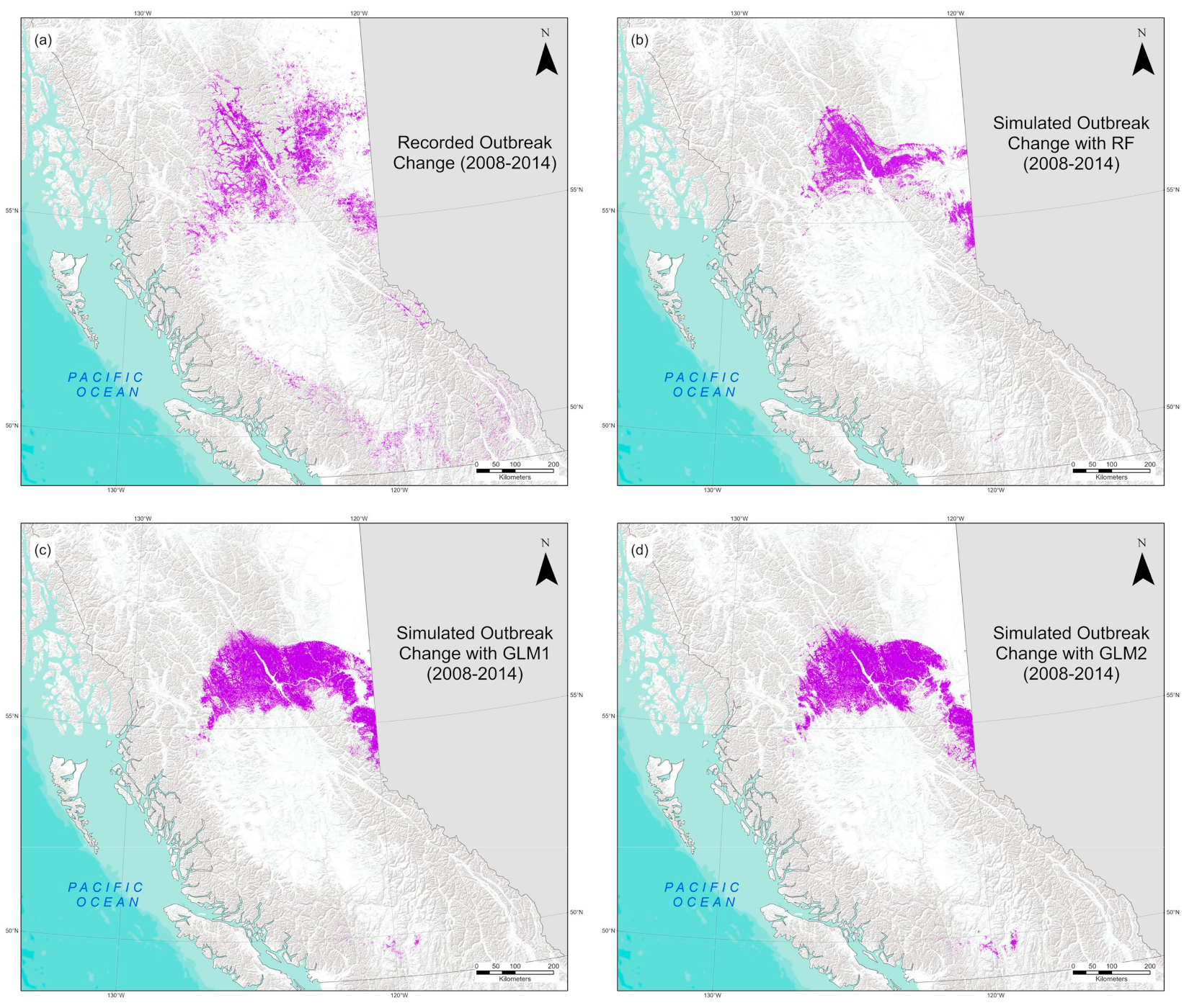
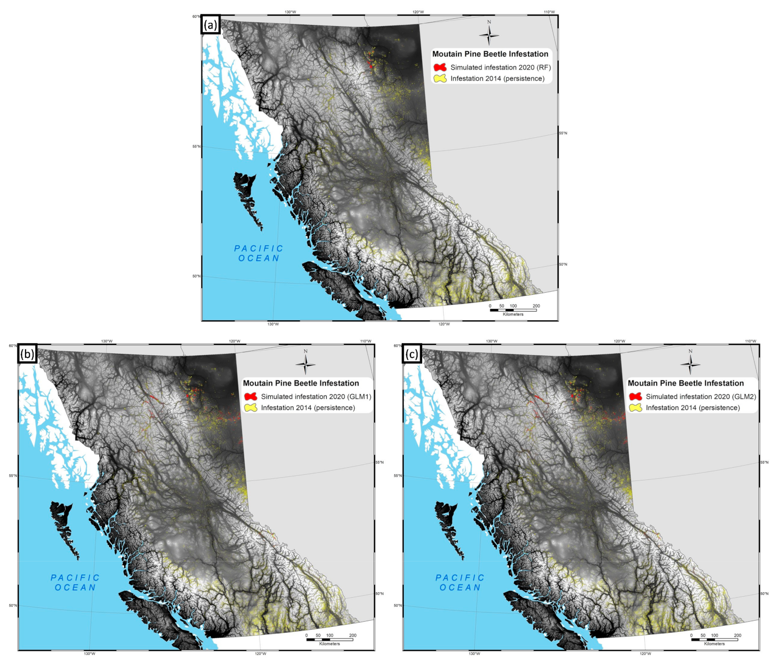
  • Simulate possible land cover changes in 2020, due to MPB infestation.

2. Materials and Methods
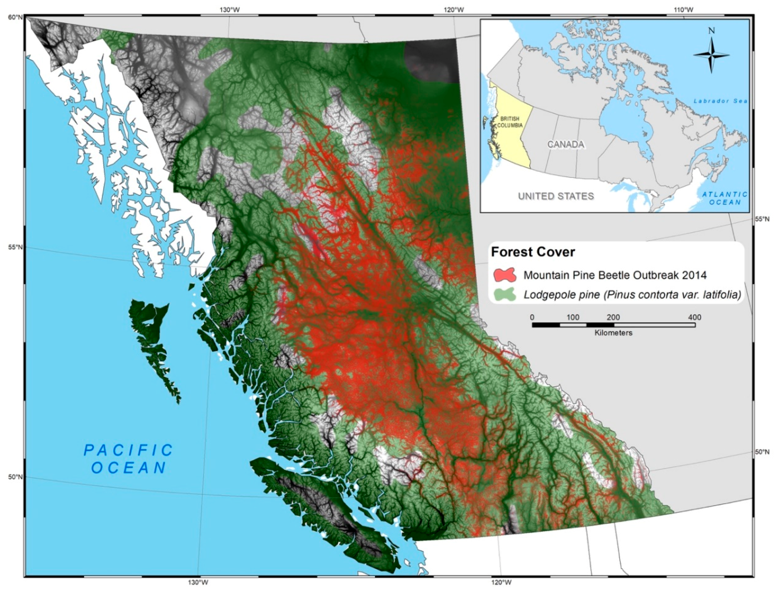
2.1. Study Area

The study was conducted in the Canadian province of British Columbia (BC), and covers an area of 944,735 km2, extending from 59°59′27″ N 138°54′19″ W to 48°59′53″ N 114°2′37″ W (Figure 1). BC is known for its highly diverse mountainous landscape subject to a diversity of disturbance regimes [39,40,41]. The climatic conditions in the province are largely controlled by the Pacific Ocean to the west, continental air masses in the interior plateaus, and the Rocky Mountains to the east [42].
Seventy percent of the total area is covered by forest, whereas only two percent of the total area is used by humans to live, cultivate, etc. Forest in central BC, where lodgepole pines are the main tree species, have been experiencing an epidemic infestation of MPB, due to factors including fire suppression and changing climate [43].

2.2. Pine Mortality Dataset

The original source of data for the project is a collection of 16 maps indicating cumulative lodgepole pine mortality caused by MPB attacks on the forests of the province as observed in the period between 1999 and 2014 [20]. Observations were acquired by the BC Ministry of Forest from aerial photographs and LANDSAT satellite images, wherein infested areas are identifiable based on their spectral response and by calculating a Normalized Difference Moisture Index (NDMI), contrasting the near-infrared (NIR) band 4, which is sensitive to the reflectance of leaf chlorophyll content, to the mid-infrared (MIR) band 5, which is sensitive to the absorbance of leaf moisture. These maps are in a raster format with an Albers equal area projection and a cell size of 400 m. The cell values equal 10 times the percentage of infestation in each cell, hence ranging from 0 to 1000; the Ministry of Forests, Lands and Natural Resource Operations of the Canadian province of BC have made this dataset publicly accessible [44]. Existing literature and reports emphasize the importance of infestation levels above which the risk of MPB attack should be considered seriously by forest managers for further investigation [44,45,46].
For the purposes of this study we applied a threshold to the cumulative infestation maps in order to transform their continuous percentage scale into a binary scale (i.e., infested = 1/not-infested = 0). This is a simplified assumption that enabled us to apply well-known statistical methods to our datasets. The procedure to calculate that threshold value is described in detail in Appendix A.

2.3. Predictor Variables

For modelling purposes, we assumed that the infestation pattern in the near future depended directly on the status of the infestation during past years. For the sake of notation, if we denote by t 2 the future year for which a prediction is sought, then t 1 represents the starting date from which the simulated map of MPB infestation is projected and t 1 p designates a previous year, for which further explanatory variables, used by the model, must be determined. Throughout the study, t 1 p < t 1 < t 2 and t 1 t 1 p = 1 year, although t 2 t 1 = 3 years.
We also assumed that the probability of beetle infestation in our thresholded maps depended entirely, for a given pixel, both on the local topography and on the state of the infestation in adjacent pixels. Arguably, local topography may either enhance or stall MPB outbreaks by, e.g., boosting or blocking beetle flights, respectively. It may also determine local climatic and environmental conditions in forests, making them a more or less suitable habitat for beetles to settle and attack. In turn, the infestation status of nearby areas should arguably have a direct influence on the number of beetles that affect a given location. These are distance-dependent variables that must be determined for every individual simulation. That dependence, however, is not known a priori and must be approximated. Bearing these ideas in mind, we set out to select a set of variables that could serve as valid drivers for the MPB infestation.
Our choices for explanatory variables represented the drivers that we fed the MPB numeric infestation model. These variables are listed in Table 1.
Topography-based explanatory variables were calculated only once at the beginning of the calibration because we assumed that local topographic conditions did not change during the time intervals spanned by the simulations:
  • Elevation: MPB infestation has been observed to take place mostly at low or medium heights [47]. Elevation is defined as height above sea level per pixel. We used a Digital Elevation Map provided by GeoBC. The original pixel size of 500 was changed to 400 to match the resolution of the MPB infestation map.
  • Slope: Steeper areas may affect, for example, distances between tree canopies on a hillside [25,48], which, in turn, may make it easier or harder for beetles to fly from one tree to another. Slope was calculated from the elevation map with the “terrain” function of the “raster” R package.
  • Aspect: The spread of the MPB infestation may benefit from milder temperatures [20,38,49] on south-oriented slopes. For that reason, aspect was calculated from the elevation map as the compass direction of the pixel slope face. We employed the “terrain” function of the “raster” R package. Next, it was sine-transformed to avoid the discontinuity at point 0–2π radians (0°–360°). Sine and cosine functions were used to avoid ambiguity at 0 radians.
  • Ruggedness: Adult beetle flight may be faster and/or longer over open ground [50]. To account for this effect, we implemented the Terrain Ruggedness Index (TRI) [51]. The TRI index was calculated from the elevation map with the “terrain” function of the “raster” R package using an 8-pixel window.
In contrast, adjacency-type predictors had to be computed at every temporal step of the simulation. As a measure of the dependence of infestation rate on the state of the neighboring pixels, we computed a weighted sum of the surrounding pixels (containing 0 s or 1 s) at each location. The basic equation to account for the adjacency effect can be written as:
z j = i ,   d i d m a x p i j · w i ,
where z j stands for the generic adjacency effect at location j . Index i runs such that the distance from location j at which pixel value p i j is summed, i.e., d i , is smaller or equal than the maximum size d m a x of the weighting window, w i . To account for the unknown true dependency, we used four different weighted sum expressions:
  • No-weighting ( z i d e n ):
    w i = 1
  • Linear weighting ( z l i n ): weights decrease linearly until d i = d m a x
    w i = d m a x d i
  • Inverse-distance weighting ( z i n v ): weights decrease as a function of the inverse of distance until d i = d m a x
    w i = 1 d i
  • Squared-inverse-distance weighting ( z s q u ): weights decrease as a function of the inverse of the squared distance until d i = d m a x
    w i = 1 d i 2
In parentheses, we have included the corresponding variable name in Equations (6) and (7) and Table 1. Appendix C demonstrates the aforementioned four weighting functions in a neighborhood of radius 5.
All of these predictor variables were determined at every infested and non-infested pixel in the t 1 p and t 1 maps. Regarding adjacency-type predictors, we included the weighted total number of surrounding infested pixels both at t 1 p and at t 1 as adjacency-type predictors. Because we ignored the exact dependence of the infestation rate on these predictors, we chose several weighting procedures to account for this unknown dependency and included all of them in the calibration procedure as independent variables.
We carried out a preliminary exploration of the relationship between infestation probability, represented by the thresholded infestation map specified above, and the set of predictor variables described in the previous paragraphs. Appendix A shows the logit-transformed average infestation as a function of the binned predictors. In general, infestation rate appears to change linearly with predictors. The mean response showed a parabolic response vs. elevation, indicating that the expected infestation rate is proportional to a quadratic function of the elevation. In addition, it displayed an approximately linear response vs. slope, aspect, ruggedness, and the log-transformed adjacency measures.

2.4. Approaches to Model and Simulate Land Cover Changes

To model and simulate the changes in the lodgepole pine forest cover within the province of BC during the sixteen-year period of the data set on recorded MPB epidemics, we implemented two algorithms: (1) generalized linear regression (GLM), and (2) random forest (RF).

2.4.1. Generalized Linear Regression (GLM)

Generalized linear regression is a maximum-likelihood regression methodology that computes the parameters of a linear model that maximize an appropriate log-likelihood [52]. It can be applied to cases where the error distribution of the response variable is not Gaussian. The linear model and the dependent variable are related directly via a continuous link function, which relates the expected value of the response variable with a linear combination of the predictors. In turn, the error distribution of the dependent variable determines our choice for the distributional model from which a log-likelihood can then be derived. There are several common options for log-likelihood and link functions, and the modeler must make his/her own choice by considering the observed relationships between response and predictor variables. The link function imposes a final expression for the log-likelihood that is often non-linear in the parameters. As a consequence, maximization of the log-likelihood is carried out iteratively with an appropriate optimization scheme (see e.g., McCullagh and Nelder, 1989).
To account for the binary dependent variable representing an MPB affected/non-affected pixel, we chose a Bernoulli log-likelihood, which corresponds to a binomial log-likelihood with number of trials equal to one. In turn, we determined the most appropriate dependence between expected binary response and the explanatory variables by carrying out an exploratory exercise (see Appendix B). Based on those observed relationships, we proposed the following linear logit link function:
l o g i t μ j = β 0 + β 1 e j + β 3 s j + β 4 a j + β 5 r j + β 6 z i d e n , t 1 + β 7 z l i n , t 1 + β 8 z i n v , t 1 + β 9 z s q u , t 1 + β 10 z i d e n , t 1 p + β 11 z l i n , t 1 p + β 12 z i n v , t 1 p + β 13 z s q u , t 1 p
l o g i t μ j = β 0 + β 1 e j + β 2 e j 2 + β 3 s j + β 4 a j + β 5 r j + β 6 z i d e n , t 1 + β 7 z l i n , t 1 + β 8 z i n v , t 1 + β 9 z s q u , t 1 + β 10 z i d e n , t 1 p + β 11 z l i n , t 1 p + β 12 z i n v , t 1 p + β 13 z s q u , t 1 p
For the sake of clarity, sub index j ( i j n , where n is the number of observations) was omitted in the neighborhood covariates z . In these equations, μ j indicates the logit-transformed expected value of the binary response variable at location j , the sub-indexed β s are the unknown parameters to be calculated, and the predictor variables are shown in Latin letters, following the notation illustrated in Table 1. In our calculations we used the “glm” function of the built-in stats package of the R software [53].
The generalized linear regression scheme described above produced a continuous function, μ , bounded between 0 and 1 such that it represented the probability of infestation. Therefore, at each location j , that probability is given by:
μ j = 1 1 + e β 0 + β 1 e j +
where the ellipsis in the exponent indicates all linear and their interactions, depending on whether we use Equation (6) or (7).
We then used μ to elaborate a predictive binary map pinpointing the location of newly infested pixels. This last step entailed the selection of a valid cut-off value to map the continuous μ variable onto a binary scale. We computed a suitable cut-off for μ by maximizing the fuzzy kappa index between observed and predicted infestation maps.

2.4.2. Random Forests (RF)

Random forests (RF) belong to the group of ensemble learning methods. Used for both classification and regression, RF are sets of decision trees each including a random subset of the data, that work based on the principle of highest voted decision, or the average of decided scores, depending on the type of the model. Throughout the calculations, we used the RF algorithms implemented in the “ranger” package of the R software. As predictor variables we used the same variables shown in Equation (6). Preliminary results (Appendix E) suggested that it was better to regress than to classify with RF, so we used the “ranger” function of that package in regression mode.

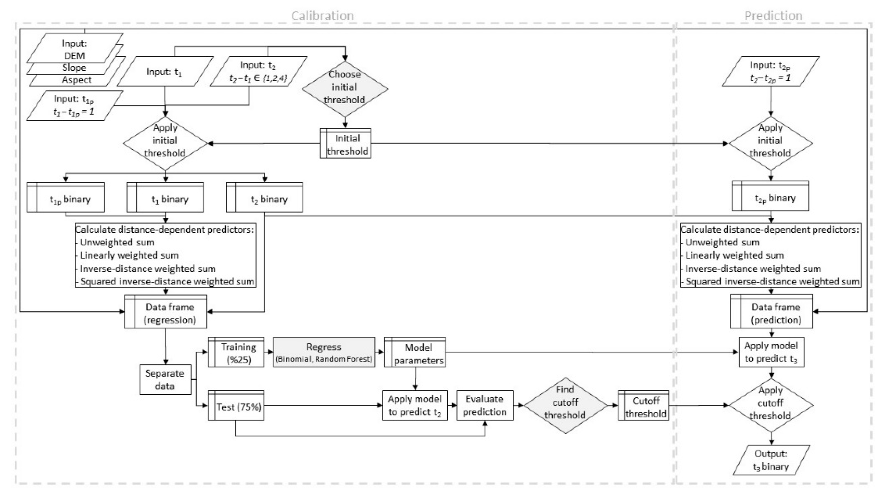
2.5. Model Calibration and Validation

To optimize the ability of our models to predict infestation in non-infested pixels we set up a cross-validation strategy by dividing the datasets into training and test subsets. The training dataset was used to calculate the unknown parameters of the model, whether binomial or RF, as shown above. The test dataset, in turn, was used to gauge the predictive ability of the models and to adjust a relevant parameter. We selected a training set containing 75% of the original dataset, whereas the test set included the remaining 25%.
Figure 2 shows the method of analysis in a flow chart. The flow of the algorithm is downwards and generally to the right. Raw inputs include geographical variables of elevation, slope, and aspect, in addition to three infestation maps. The time interval between the first two maps at t 1 p and t 1 is one year, and the time step between the last two maps between t 1 and t 2 is 3 years. The goal of the algorithm is to predict the binary spread of infestations in the next time step. After reading inputs, the algorithm is divided into two main parts. In the first part, the inputs are analyzed, and a model is developed and parameterized to simulate the change from the first two images ( t 1 p and t 1 maps) to the third ( t 2 ). In the second part, the parameterized model is used to predict the change from the last two given images ( t 2 p and t 2 maps) to the next time step in the future ( t 3 ).
In this model, parameters were determined and adjusted in three stages. These stages are shown with gray flowchart shapes in Figure 2. First, the initial threshold for conversion of numeric data into binary (infested/not infested) was identified. The input images were converted to binary assuming a threshold of 0.1586553 (see Appendix A), i.e., infestation proportions of above 0.158 are taken as presence and lower values as non-presence. The second stage was the adjustment of the regression model parameters. To do so, the compiled dataset was divided into training and test datasets. Using the training dataset, regression parameters were estimated. This preliminary model was then applied to the test dataset in order to assess its ability to predict the changes in input data. Such assessment involved the third stage of model parameterization—the selection of the final threshold for creation of the binary output. This was done by applying and testing the goodness-of-fit of 1000 images created by different cut-off values. The test involved giving test data to the model and comparing its output with the most recent input image. The cut-off thresholds giving the highest kappa and the highest Youden’s J statistic was selected for application in the prediction phase.
Model output was compared with the reference data for validation. It should be noted that the similarity of simulation and reference maps of the final year does not provide sufficient information for validating the model [54,55,56]. In fact, if the overall change in the landscape is small, even an erroneous prediction can still be highly similar to the reference. Therefore, model validation should account for the simulated and observed change. This requires considering three maps: a reference map of the beginning time, and reference and simulation maps at the ending time. In this study, the process of change is infestation, which is irreversible. As such, change may only occur in areas that were initially not infested. We analyzed these areas when validating the model.

2.6. Software

Calibration and simulation algorithms were computed using R 3.6.0 (Auckland, New Zealand) [53] and cartography was produced using ArcGIS Pro 2.4 (Redlands, CA, USA) [57].

3. Results

Validation testing of the model involved simulation of changes in the study area from 2008 to 2014 and comparison with reference observations. Prior to testing, the model was parameterized using data of changes from 2005 to 2008. Then, in two rounds, it simulated the change from 2008 to 2011 and from the predicted 2011 to 2014. These predictions were made with 3-year time steps. Figure 3 shows model results for three algorithms—binomial regression (Equation (6); hereafter GLM1), binomial regression with parabolic elevation (Equation (7); hereafter GLM2), and random forest (RF) with maximum kappa final cut-off threshold—in addition to the observed change. (Appendix D)
Outputs of validation analysis for the three algorithms with maximum kappa final cut-off threshold are presented in Figure 4. Each map of this figure corresponds to one simulation algorithm and demonstrates a comparison between three images: observed infestations in 2008, simulated infestations in 2014, and observed infestations in 2014. In this figure, correctly simulated changes are identified as “hits”; observed changes that are missing from simulations are identified as “misses”; simulated changes that are not observed are identified as “false alarms”; and correct simulations of no change are identified as “correct rejections”. Because infestation is a one-way process that is not reversible, it is evident that zones of “prior infestation”, that is, zones that were already infested at the beginning of the study period, are not susceptible to future change and they should be excluded from the assessment of model performance.
Table 2 shows hits, misses and false alarms in numbers of pixels for each of the simulation algorithms. In addition, this table gives the figure of merit, which is the percentage of hits in the sum of hits, misses, and false alarms. The table also shows the overall accuracy of each model, which is the percentage of correct predictions in the study area.
Using the model results, which indicate locations of simulated infestations and the Ministry’s map of pine volume density [58] in the study area, cumulative estimates of pine volume killed were calculated for each algorithm. Table 3 shows these estimates. In comparison, the real percentage of cumulative change based on the Ministry’s map of observed infestations for year 2014 is 49% for the entire province (excluding the Tree Farm License Zone).
Figure 5 shows simulations of changes from 2014 to 2020, where the model was parameterized with observed changes from 2011 to 2014. The time step for all these simulations was 3 years. This is a demonstration of a possible application of the model for future predictions. Model outputs are projections of the infestations in the future, for which no reference data is available yet. As such, it is not possible to calculate the accuracy of these predictions. Rather, based on the results of validation tests described above and summarized in Table 2, we assume that the model is able to produce valid predictions. Aggregate percentages of cumulative pine volume killed are estimated for each simulation algorithm using the Ministry’s pine volume density map, and are presented in Table 4.

4. Discussion

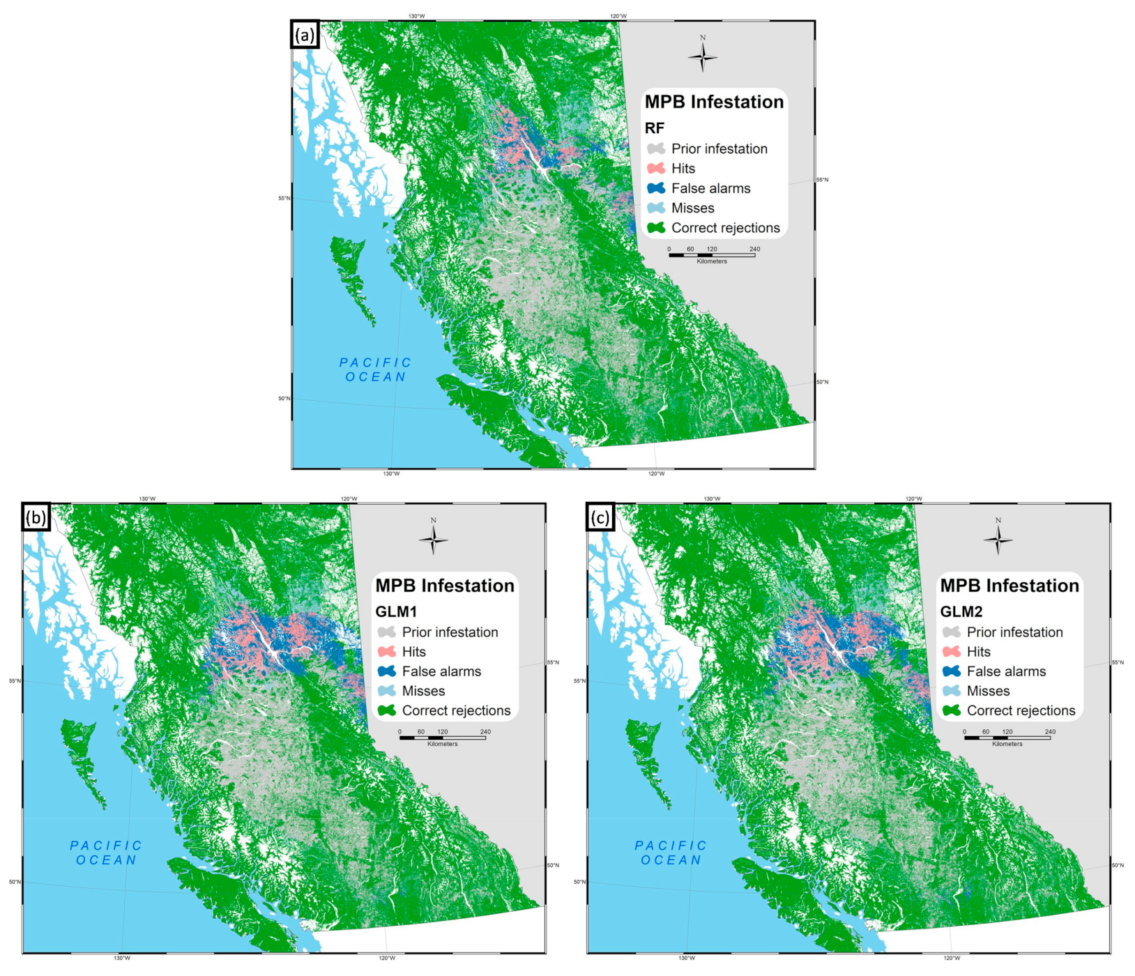
4.1. Model Validation

All of the simulation and observation images show a noticeable area of new infestations north of the center. A closer examination also reveals scattered infestations in other regions. Regarding the larger infested area, we know based on prior information that it is the result of the spread of previous infestations from the center of the province towards the north. A visual inspection suggests that, in the two GLM simulations, the southern and northern envelopes of the large infested areas are somewhat similar, as if the models have offset the prior infestations to the north. Considering that the model calculates the adjacency-type predictors in windows of a predefined size, it appears from Figure 4 that the GLM algorithms predicted a large number of infestations in a limited distance.
Comparing the images with respect to the large zone of new infestations north of the center, it appears that the GLM algorithms predicted a larger area for the spread of the insect. Moreover, the two GLM algorithms appear to have predicted a more relatively uniform spread inside the zone of new infestations. In contrast, the reference observation image shows a less homogeneous pattern in the same area. Regarding the RF algorithm, its result is somewhat non-homogeneous in that area. However, identifying correspondence between this image and the reference observation requires further analysis.
Figure 4 clearly shows that the larger parts of observed and simulated changes occurred in the area north of the center. It is noticeable that the two GLM algorithms predicted larger numbers of infestations in this area. Some of these predictions of infestation matched reference observation (hits), but many of them did not (false alarms). False alarms in the results of these two algorithms are visually distinctive. In contrast, the RF algorithm predicted a smaller spread of infestations and missed some infestations that actually occurred.
Table 2 reveals useful information about the performance of the models. Considering that hits indicate correct predictions of change, and that misses and false alarms indicate errors in prediction of change, the figure of merit is the proportion of correct predictions in all predictions involving change. This table confirms the above visual analyses of simulation outputs. The GLM algorithms predicted more change (hits + false alarms) than RF. Some of these excess predictions were correct, and these algorithms had more hits than RF. However, many of them were incorrect. The GLM algorithms, especially with Youden’s J final cutoff threshold, produced a large number of false alarms. In fact, although they have more hits and therefore higher figures of merit, this advantage is overshadowed by their error in estimating the quantity of change. The GLM algorithms, particularly with Youden’s J final cutoff threshold, produced more false alarms than misses. This means that they overestimated the quantity of change. In contrast, the table shows that the RF algorithm underestimated the quantity of change, producing more misses than false alarms. With the kappa final cutoff threshold, the number of these errors in the estimation of quantity in RF is comparable with that of the GLM algorithms. With Youden’s J final cutoff threshold, however, the underestimation of the quantity of change in the RF algorithm is relatively small.
Prior to producing prediction maps, each algorithm creates a probability map. Then it compares that map with the final cutoff threshold; that is, it classifies pixel values above the final cutoff threshold as ‘Infested’, and others as ‘Not infested’. The Youden’s J threshold was calculated to be lower value than that of the Kappa threshold for each algorithm. Therefore, for the same probability map, Youden’s J cutoff predicts more infestations than the kappa cutoff. On the other hand, the table shows that regardless of the final cutoff threshold, the GLM algorithms tend to predict more change. This tendency, combined with the lower Youden’s J final cutoff threshold, resulted in the large overestimation of quantity seen in the 2nd and 4th rows of the table. One avenue for improvement of the model in future works can be to reduce its error of estimated quantity of change.
As seen in Table 3, the random forest algorithm produces a closer estimate of the aggregate quantity of change in the study area. In comparison, the other two algorithms (GLM1 and GLM2) appear to overestimate this quantity. This is also confirmed in Table 2 and Figure 4; it may be noted that these algorithms produce more false alarms than misses. Having seen the model’s performance in the validation test, it is easier to understand the model’s prediction of future changes.

4.2. Model Predictions

Predictions of future infestations are summarized in Table 4. These calculations are based on the Ministry’s previous inventory and do not include the effect of harvesting or management decisions. Different simulations estimate that by 2020 between 64 and 70 percent of the pine volume in BC forests will be killed in MPB attacks. These assessments have been made for the entire forests—or the Whole Land Base (WLB)—of the province. The Ministry has made estimates of the spread of infestation in the Timber Harvesting Land Base (THLB), which is a smaller subset of the WLB. According to the Ministry the cumulative percentage of pine volume killed in the THLB could reach 55% by 2020 (BC Ministry of Forests, 2015c). Taking this difference in land base or study area into account, the results of our model can be considered as a complement to the Ministry’s calculations, particularly for zones outside the THLB. In both studies, it is predicted that in future the spread of infestations in the province will subside.

4.3. Limitations of the Study

Applying a threshold to transform the initial continuous infestation maps into binary maps may entail a loss of information because we discard valid knowledge about the shape of the infestation curve, i.e., whether it grows faster or slower until it reaches saturation. However, we have shown (Appendix A) that, in general, infestation curves in all pixels seem to follow a similar sigmoidal pattern. Therefore, our choice of a single threshold to compute all binary maps appears to be a reasonable compromise between simplifying the analysis and retaining as much information relating to the infestation process as possible.
It is obvious that, for a process that spreads spatially, the state of the surroundings is important in determining the expansion rate. Presumably, definitions of adjacency other than those we used in the present study may lead to a better characterization of the infestation. Proximity laws based on insect phenology (e.g., flight time and strength, sensibility to extreme heat or sunlight) may yield better results than the generic adjacency functions used in this work. Future work may shed some light on this crucial topic.

5. Conclusions

In this work, we built a spatial change model by integrating neighborhood selection and transition rule identification in one process. Although we did not have detailed information about distance and neighborhood effects of MPB infestations at the beginning of this study, we compensated for this lack of knowledge by calculating several mathematically independent functions of distance as predictors in the model, and allowed the rule identification algorithm to find the transition rule that best described the input data. We validated our model by comparison of its output with the observed data. Validation based on components of figure of merit gave us better insight into the performance of different algorithms applied in the model. In validation analyses, we noted that although the GLM simulations resulted in higher figures of merit, the RF algorithm was better able to estimate the quantity of change. We then used the validated model to predict the upcoming changes in the study area. By integrating neighborhood effects as variables in the parameterization of the model, we were able to simulate spatiotemporal complexities of a forest land change process.

Author Contributions

Conceptualization, L.P., R.M.-H. and S.H.; methodology, L.P., R.M.-H. and S.H.; software, R.M.-H. and S.H.; validation, L.P. and S.H.; formal analysis, L.P., R.M.-H. and S.H.; investigation, L.P., R.M.-H. and S.H.; resources, L.P., R.M.-H. and S.H.; data curation, S.H.; writing—original draft preparation, L.P., R.M.-H. and S.H.; writing—review and editing, L.P., R.M.-H. and S.H.; visualization, L.P. and S.H.; supervision, L.P. and R.M.-H.; project administration, L.P.; funding acquisition, L.P. and R.M.-H. All authors have read and agreed to the published version of the manuscript.

Funding

This research was partially funded by the Natural Sciences and Engineering Research Council (NSERC) of Canada through the Discovery Grant number RGPIN/05396–2016 awarded to LP. RMH received financial support from the European Union’s Seventh Framework Programme through NEWFOREST programme number PIRSES-GA-2013–612645.

Acknowledgments

We are thankful to two anonymous reviewers who helped improve this paper. We are thankful to the Université de Montréal’s International Affairs Office (IAO) for their financial support trough the International Partnership Development program, which allowed the collaboration between researchers from UdeM and CREAF. We are also thankful to Graham Hawkins from the Ministry of Forests, Lands and Natural Resource Operations of British Columbia for his support in providing data, and to the Netherlands Environmental Assessment Agency (MNP) as the owner and RIKS BV as the developer of the Map Comparison Kit for providing access to the software. The analyses were made possible thanks to provision of high-performance computing by Calcul Quebec.

Conflicts of Interest

The authors declare no conflict of interest. The funders had no role in the design of the study; in the collection, analyses, or interpretation of data; in the writing of the manuscript, or in the decision to publish the results.

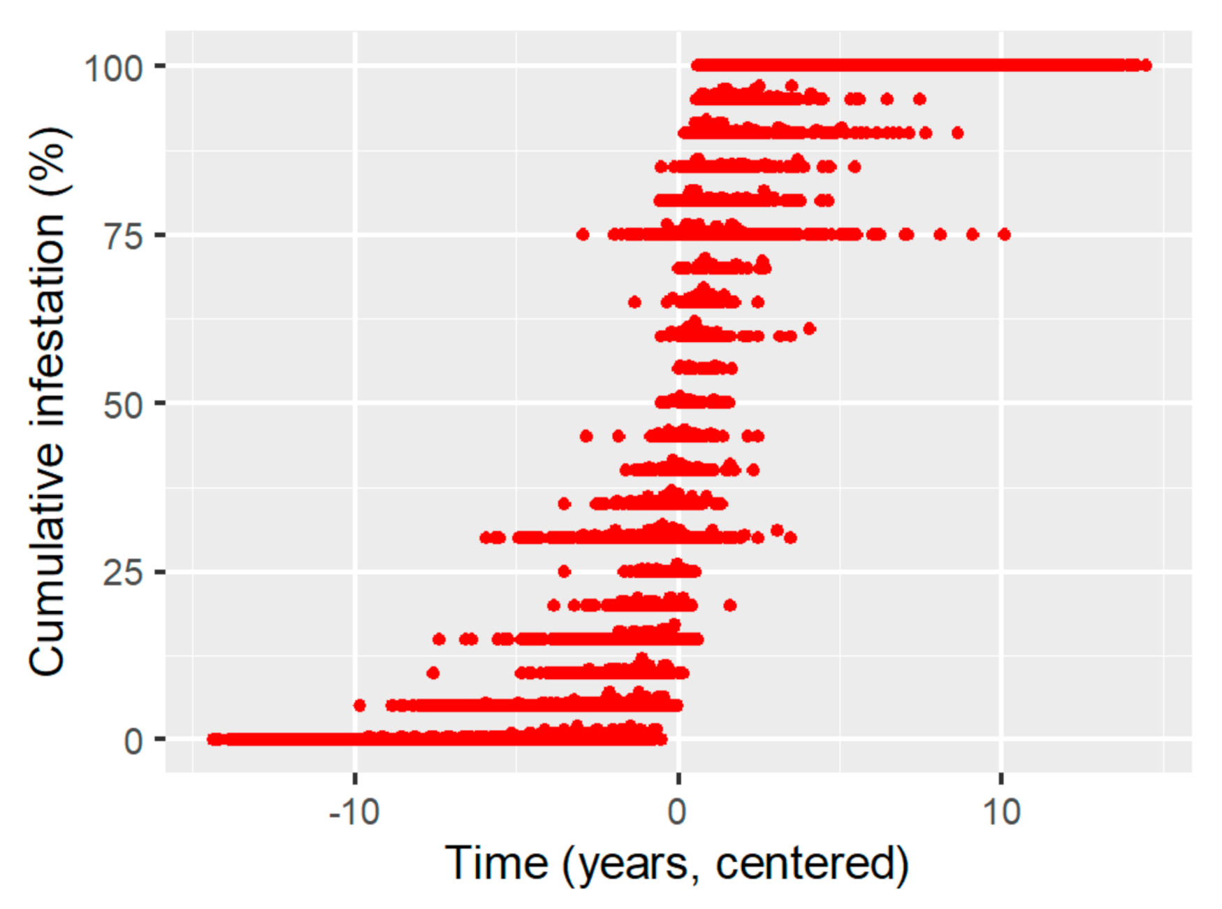
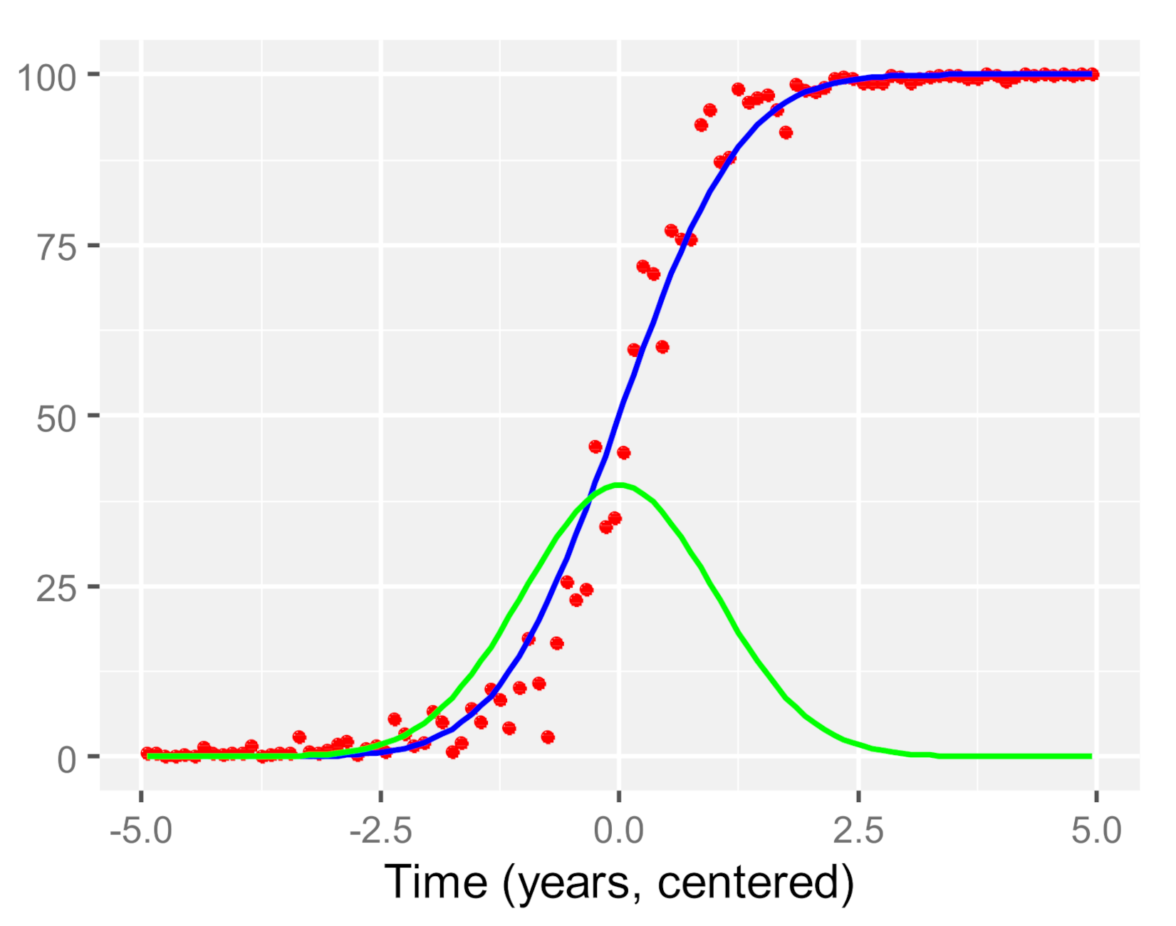
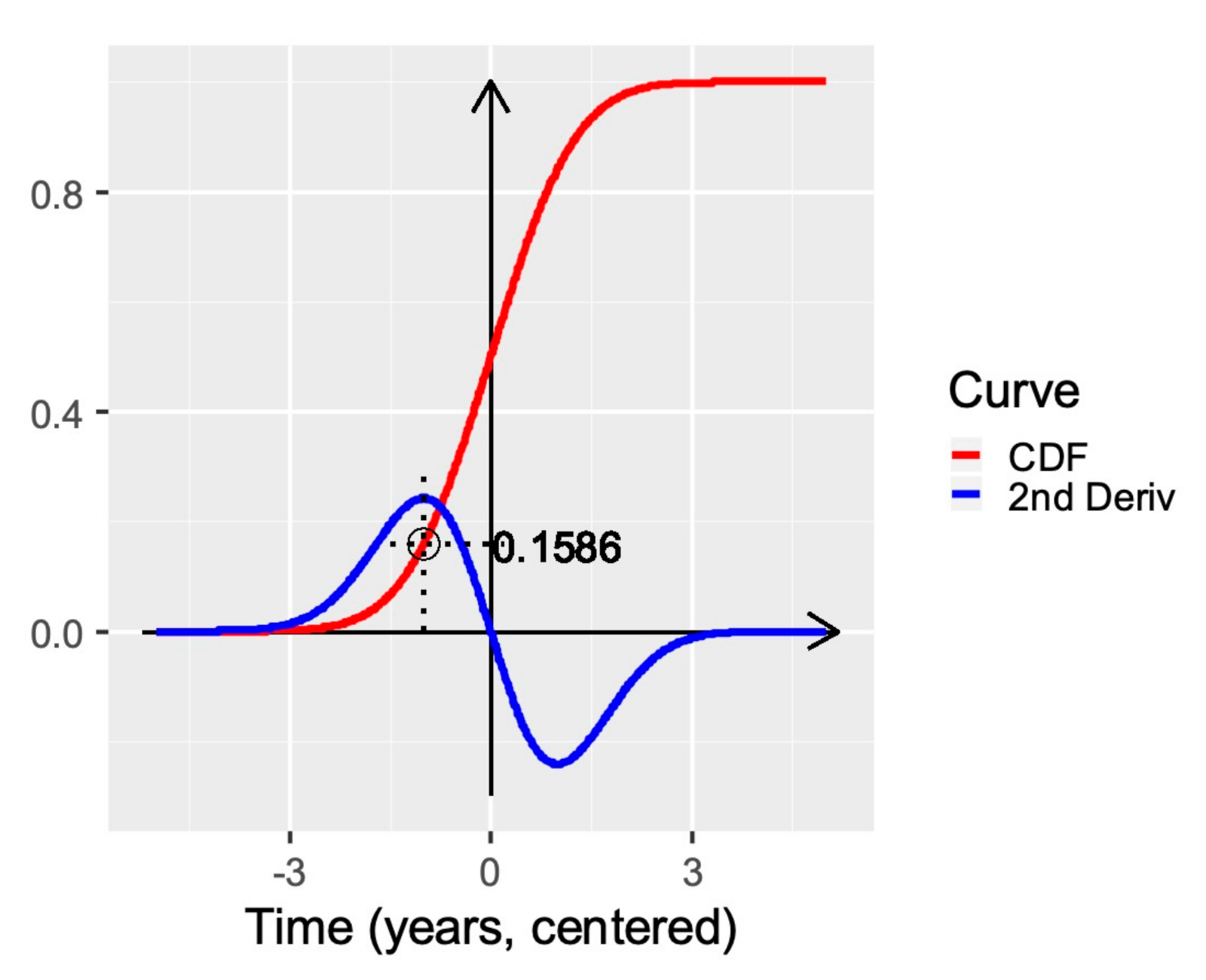
Appendix A. Calculation of Threshold Value on Cumulative Pinus contorta Mortality Data

To calculate the initial threshold value (i.e., the cutoff value that we must apply to the original infestation map), we first convert the original 0–1000 scale of the cumulative data into a 0%–100% scale. At every spatial pixel the infestation starts at a value close to 0% starting in the year 1999, which then increases quickly and finally arrives at saturation level (that is, there are no more trees left in that pixel to attack) near 100%. When sample curves of the cumulative infestation values are plotted as a function of time (see examples in Figure A1, left panel) we see that they approximately display a sigmoidal behavior, although the years the infestation starts are different.
Figure A1. Three sample curves of cumulative (left panels) and annual (right panels) infestation percentages.
Forests 11 01215 g0a1
Next, we determine the annual infestation percentage by computing the numerical derivative of the cumulative curves. The resulting curves (Figure A1, right panel) now show a coarse bell-like shape with a given center and width.
If we conjecture that the curves represent unimodal and symmetric distributions, we can calculate, at each pixel i , (a) the centroid c i as the first statistical moment, and (b) a proxy of the width w i as the square-root of second moment (i.e., variance), as follows:
c i = j = 1 16 p i j · t j j = 1 16 p i j
and:
w i = j = 1 16 p i j · t j c i 2 j = 1 16 p i j
where p i j stands for the infestation percentage for pixel i at year t j ( t 1 = 1999 , , t 16 = 2014 ) . We then use centroids c i to re-center the offset of the original cumulative infestation curves. A random selection of 50,000 offset-corrected cumulative curves is shown in Figure A2. This figure shows the resulting re-centered data points, where it is now easier to make out an approximate sigmoidal shape for the cumulative infestation process. Notice that no correction for different widths has been carried out.
Figure A2. Offset-corrected cumulative infestation data points.
Forests 11 01215 g0a2
Next, we compute the mean cumulative infestation in small intervals along the temporal axis. When those mean infestation data points are plotted as a function of time (Figure A3, red dots), the sigmoidal-like shape of the infestation process becomes more conspicuous. Finally, we plot a normal cumulative distribution function (CDF, hereafter I t ) with standard deviation σ = w ¯ (Figure A3, blue curve), where:
w ¯ = 1 N · i = 1 N w i
Figure A3. Mean observed and offset-corrected cumulative infestation (red dots), normal cumulative distribution function I t (CDF, in blue, scaled to 0–100), whose standard deviation is explained in text, and its derivative I t , i.e., the normal probability density function (in green).
Forests 11 01215 g0a3
For reference, we have also plotted (in green) the probability density function of the corresponding normal distribution, I t , in Figure A3. Clearly, I t serves as a good approximation to the observed cumulative infestation curve. In curves I t and I t we can distinguish five phases as we move from left to right:
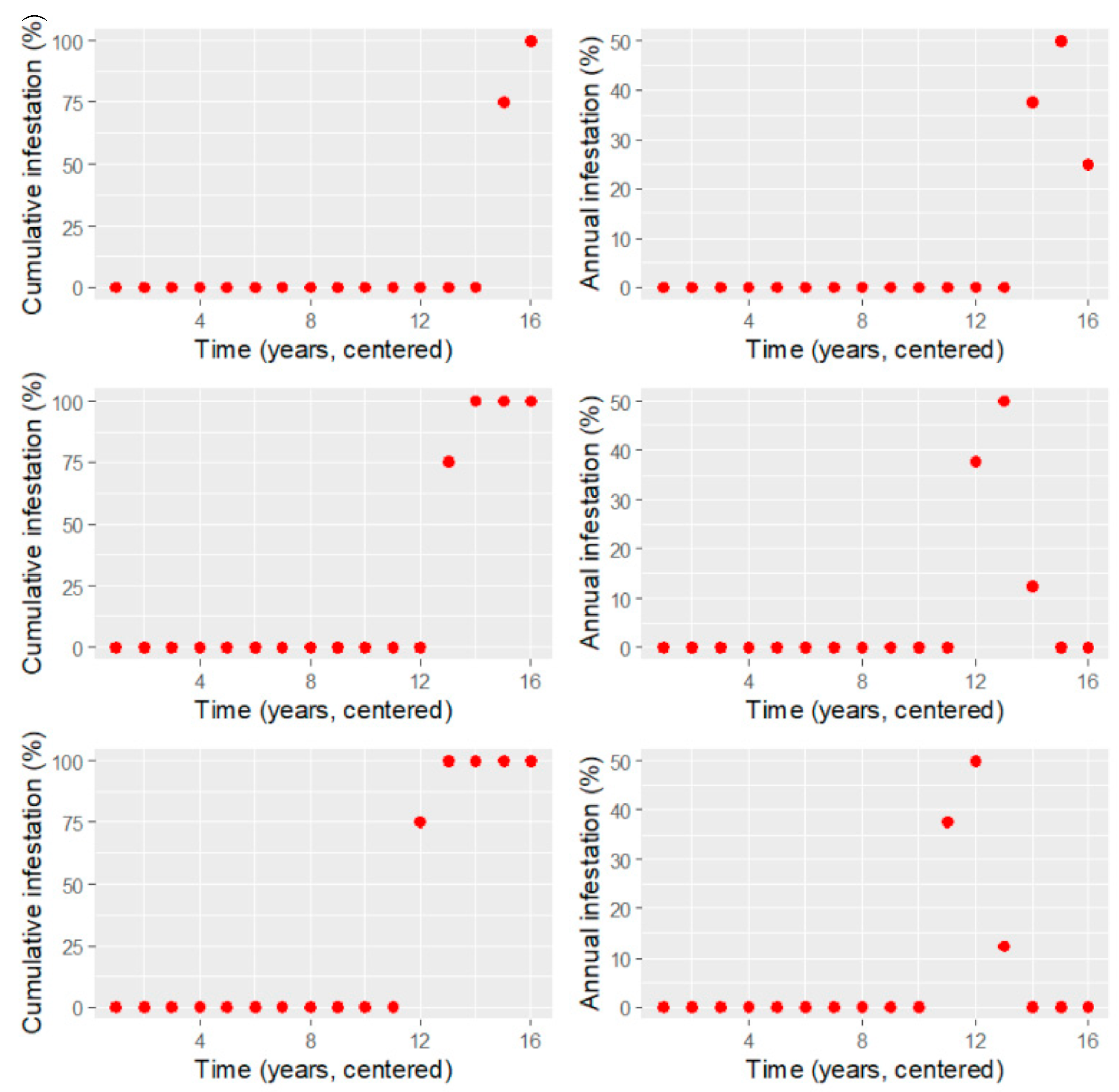
  • initial negligible or very low infestation that spreads slowly ( I t and I t are close to zero);
  • a transitional phase in which the infestation starts picking up speed ( I t still low but I t increases);
  • fast but steady infestation that increases constantly ( I t increases but I t reaches a maximum);
  • transitional phase during which the infestation slows down ( I t increases further, I t decreases);
  • saturation level ( I t highest, I t very close to zero).
We assume in the present study that a critical moment in the spread of the infestation occurs when, in phase 2 above, the infestation starts picking up speed, therefore accelerating its spread. Consequently, we will use the infestation level at which that acceleration is maximum as our threshold value I t h , which will enable us to categorize the continuous cumulative infestation maps into binary maps I b such that:
I b = 0   n o t   i n f e s t e d I I t h 1   i n f e s t e d I > I t h
The so-called acceleration can be calculated as the second derivative of I t . Therefore, to find its maximum we must compute in turn the third derivative and solve I t = 0 . Assuming that I t is well approximated by a normal CDF, we know that, for a centered normal distribution:
I t = t 2 σ 2 · e t 2 2 σ 2 σ 5 · 2 π
Equating I t = 0 we arrive at t = ± σ , excluding the trivial solutions t = ± . Because t = + σ corresponds to phase 4 above, i.e., the deaccelerating phase, we take t t h = σ as the temporal location of the sought-after threshold. Inserting t t h into I t yields, finally, I σ = 0.1586553 (or 15.86553 in our percentage scale). Figure A4 depicts the procedure.
Figure A4. Cumulative distribution function (red) of the normal distribution and its 2nd derivative (blue). The location of the maximum of the 2nd derivative and the corresponding ordinate is indicated with a dashed line.
Forests 11 01215 g0a4

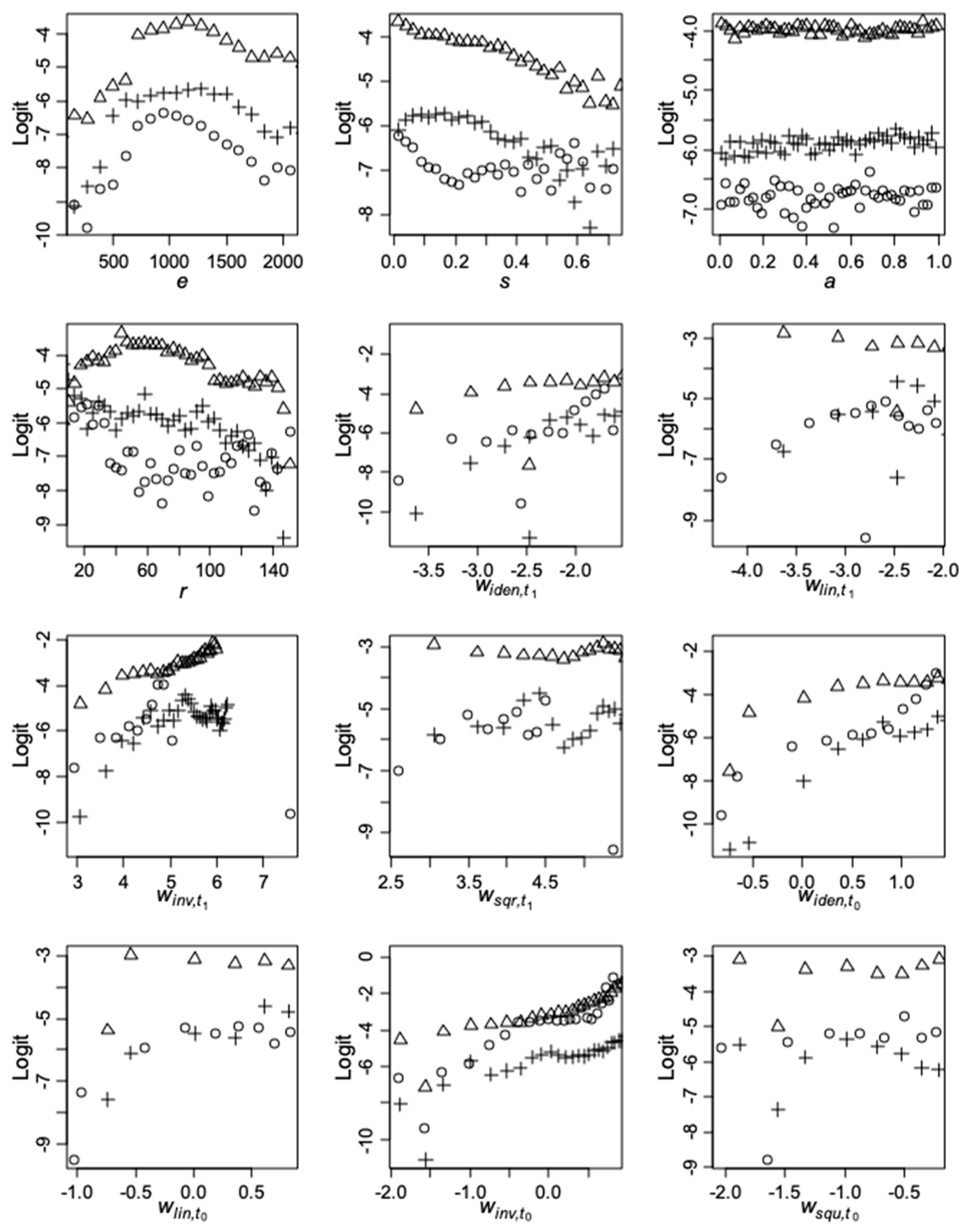
Appendix B. Plots of Average Mortality vs. Predictors

Each predictor variable in Table 1 (see main text) was binned at consecutive intervals and at each interval we averaged over the corresponding 0 and 1 pixels in the map. This yielded the expected infestation rates, which were then logit-transformed and plotted vs. the center of the intervals, as shown below.
Figure A5. Plots of average mortality vs. predictors in three transition periods: 2001–2002 (circles), 2007–2008 (triangles), and 2013–2014 (plus signs).
Forests 11 01215 g0a5

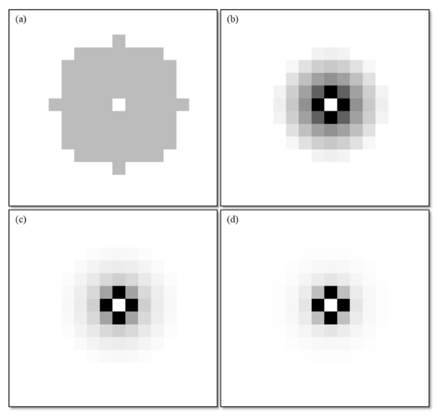
Appendix C. Graphic Representation of the Four Different Neighborhood Types Implemented

Figure A6. The four neighborhood types implemented in this model are (a) no-weight: neighborhood effect is uniformly distributed; (b) linear: neighborhood effect decreases linearly with increasing distance; (c) inverse-distance: neighborhood effect decreases inversely proportional to distance; and (d) squared-inverse-distance: neighborhood effect decreases inversely proportional to distance squared.
Forests 11 01215 g0a6

Appendix D. Model Parameterization

The results of parameterization of the GLM1, GLM2, and RF models are summarized in this appendix.
The GLM1 algorithm resulted in a Receiver Operating Characteristic Area Under Curve (AUC) of 0.7802905. The maximum values of kappa and Youden’s J obtained in model parameterization were 0.3489783 and 0.4540825, respectively. Statistics for this model’s variables are presented in Table A1.
Table A1. Parameterization statistics for the GLM1 model.
VariableAcronymEstimateStd. Errorz ValuePr (>|z|)
(Intercept)-−2.5189277.437363 × 10−3−338.6854880.000000
elevation e 2.415789 × 10−45.497418 × 10−643.9440720.000000
ruggedness r 3.418483 × 10−43.661161 × 10−59.3371579.895502 × 10−21
aspect.sin (sine) a −1.249106 × 10−22.968032 × 10−3−4.2085342.570333 × 10−5
aspect.cos (cosine) a −8.139534 × 10−32.982952 × 10−3−2.7286846.358761 × 10−3
slope s −2.6823641.821996 × 10−2−147.2211460.000000
identity.1 z i d e n , t 1 p −2.990441 × 103.971936 × 10−1−75.2892570.000000
linear.1 z l i n , t 1 p 6.979188 × 10−61.514023 × 10−746.0969670.000000
inverse.1 z i n v , t 1 p −3.289507 × 10−21.136399 × 10−3−28.9467553.083004 × 10−184
squared.1 z s q u , t 1 p −9.227856 × 10−24.722606 × 10−3−19.5397525.042652 × 10−85
identity.2 z i d e n , t 1 3.895161 × 103.035022 × 10−1128.3404460.000000
linear.2 z l i n , t 1 −6.558742 × 10−61.114139 × 10−7−58.8682330.000000
inverse.2 z i n v , t 1 1.187859 × 10−28.019164 × 10−414.8127531.211739 × 10−49
squared.2 z s q u , t 1 1.341532 × 10−13.245616 × 10−341.3336590.000000
The GLM2 algorithm resulted in an AUC of 0.7966494. The maximum values of kappa and Youden’s J obtained in model parameterization were 0.3603257 and 0.4610181, respectively. Statistics for this model’s variables are presented in Table A2.
Table A2. Parameterization statistics for the GLM2 model.
VariableAcronymEstimateStd. ErrorZ ValuePr (>|z|)
(Intercept)-−5.7921892.340479 × 10−2−247.4787800.000000
elevation e 6.035065 × 10−33.824616 × 10−5157.7953490.000000
ruggedness r 9.025530 × 10−43.765714 × 10−523.9676496.049586 × 10−127
aspect.sin (sine) a −1.940276 × 10−22.988868 × 10−3−6.4916778.488584 × 10−11
aspect.cos (cosine) a −8.848104 × 10−32.996480 × 10−3−2.9528333.148722 × 10−3
slope s −2.4949521.827487 × 10−2−136.5236260.000000
identity.1 z i d e n , t 1 p −3.198807 × 103.989017 × 10−1−80.1903640.000000
linear.1 z l i n , t 1 p 6.664911 × 10−61.514503 × 10−744.0072610.000000
inverse.1 z i n v , t 1 p −2.847800 × 10−21.135279 × 10−3−25.0845827.326996 × 10−139
squared.1 z s q u , t 1 p −9.944317 × 10−24.717755 × 10−3−21.0784951.253054 × 10−98
identity.2 z i d e n , t 1 3.926965 × 103.044064 × 10−1129.0040150.000000
linear.2 z l i n , t 1 −6.281823 × 10−61.115482 × 10−7−56.3148880.000000
inverse.2 z i n v , t 1 1.006898 × 10−28.026541 × 10−412.5446074.255184 × 10−36
squared.2 z s q u , t 1 1.190556 × 10−13.241775 × 10−336.7254552.866455 × 10−295
I(elevation^2) e 2 −2.332311 × 10−61.521917 × 10−8−153.2482430.000000
The RF algorithm resulted in an AUC of 0.9999999. The maximum values of kappa and Youden’s J obtained in model parameterization were 0.9996198 and 0.9997796, respectively. The RF algorithm produces relative importance ranks for model variables. These ranks are presented in Table A3, with the most important variable given the score of 100.
Table A3. RF model variable ranks and relative importance scores rounded to two decimal digits.
VariableAcronymRelative Importance Score
inverse.2 z i n v , t 1 100.00
identity.2 z i d e n , t 1 99.96
linear.1 z l i n , t 1 p 90.85
inverse.1 z i n v , t 1 p 90.23
linear.2 z l i n , t 1 80.11
identity.1 z i d e n , t 1 p 75.00
squared.1 z s q u , t 1 p 74.04
squared.2 z s q u , t 1 61.32
elevation e 22.43
slope s 11.16
aspect.cos (cosine) a 6.95
aspect.sin (sine) a 6.76
ruggedness r 3.83

Appendix E. Code and Data Availability

Model code is available at https://github.com/s-harati/model-MPB. Data used in the study is accessible at https://doi.org/10.17605/OSF.IO/V7ATJ.

References

  1. McCullough, D.G.; Werner, R.A.; Neumann, D. Fire and Insects in Northern and Boreal Forest Ecosystems of North America. Annu. Rev. Entomol. 1998, 43, 107–127. [Google Scholar] [CrossRef] [PubMed] [Green Version]
  2. Bourbonnais, M.L.; Nelson, T.A.; Wulder, M.A. Geographic analysis of the impacts of mountain pine beetle infestation on forest fire ignition. Can. Geogr. Géographe Can. 2014, 58, 188–202. [Google Scholar] [CrossRef]
  3. Robbins, J. Bark Beetles Kill Millions of Acres of Trees in West-NYTimes.com. New York Times, 17 November 2008. [Google Scholar]
  4. Axelson, J.N.; Alfaro, R.I.; Hawkes, B.C. Changes in stand structure in uneven-aged lodgepole pine stands impacted by mountain pine beetle epidemics and fires in central British Columbia. For. Chron. 2010, 86, 87–99. [Google Scholar] [CrossRef]
  5. MacLean, D.A. Impacts of insect outbreaks on tree mortality, productivity, and stand development. Can. Entomol. 2016, 148, S138–S159. [Google Scholar] [CrossRef] [Green Version]
  6. Pelz, K.A.; Smith, F.W. Thirty year change in lodgepole and lodgepole/mixed conifer forest structure following 1980s mountain pine beetle outbreak in western Colorado, USA. For. Ecol. Manag. 2012, 280, 93–102. [Google Scholar] [CrossRef]
  7. Herms, D.A.; McCullough, D.G. Emerald ash borer invasion of North America: History, biology, ecology, impacts, and management. Annu. Rev. Entomol. 2014, 59, 13–30. [Google Scholar] [CrossRef] [Green Version]
  8. Sturtevant, B.R.; Achtemeier, G.L.; Charney, J.J.; Anderson, D.P.; Cooke, B.J.; Townsend, P.A. Long-distance dispersal of spruce budworm (Choristoneura fumiferana Clemens) in Minnesota (USA) and Ontario (Canada) via the atmospheric pathway. Agric. For. Meteorol. 2013, 168, 186–200. [Google Scholar] [CrossRef]
  9. Patriquin, M.N.; Wellstead, A.M.; White, W.A. Beetles, trees, and people: Regional economic impact sensitivity and policy considerations related to the mountain pine beetle infestation in British Columbia, Canada. For. Policy Econ. 2007, 9, 938–946. [Google Scholar] [CrossRef]
  10. Chang, W.-Y.; Lantz, V.A.; Hennigar, C.R.; MacLean, D.A. Economic impacts of forest pests: A case study of spruce budworm outbreaks and control in New Brunswick, Canada. Can. J. For. Res. 2012, 42, 490–505. [Google Scholar] [CrossRef]
  11. Corbett, L.J.; Withey, P.; Lantz, V.A.; Ochuodho, T.O. The economic impact of the mountain pine beetle infestation in British Columbia: Provincial estimates from a CGE analysis. Forestry 2016, 89, 100–105. [Google Scholar] [CrossRef] [Green Version]
  12. Petersen, B.; Stuart, D. Explanations of a changing landscape: A critical examination of the British Columbia bark beetle epidemic. Environ. Plan. A 2014, 46, 598–613. [Google Scholar] [CrossRef]
  13. Flint, C.G.; McFarlane, B.; Müller, M. Human dimensions of forest disturbance by insects: An international synthesis. Environ. Manag. 2009, 43, 1174–1186. [Google Scholar] [CrossRef]
  14. Strohm, S.; Reid, M.L.; Tyson, R.C. Impacts of management on Mountain Pine Beetle spread and damage: A process-rich model. Ecol. Model. 2016, 337, 241–252. [Google Scholar] [CrossRef]
  15. James, P.M.A.; Huber, D.P.W. TRIA-Net: 10 years of collaborative research on turning risk into action for the mountain pine beetle epidemic. Can. J. For. Res. 2019, 49, iii–v. [Google Scholar] [CrossRef]
  16. Bone, C.; Nelson, M.F. Improving Mountain Pine Beetle Survival Predictions Using Multi-Year Temperatures Across the Western USA. Forests 2019, 10, 866. [Google Scholar] [CrossRef] [Green Version]
  17. Safranyik, L.; Carroll, A. The biology and epidemiology of the mountain pine beetle in lodgepole pine forests. In The Mountain Pine Beetle: A Synthesis of Biology, Management, and Impacts on Lodgepole Pine; Safranyik, L., Wilson, W.R., Eds.; Natural Resources Canada, Canadian Forest Service, Pacific Forestry Centre: Victoria, BC, Canada, 2007; pp. 3–66. [Google Scholar]
  18. Bentz, B.J.; Boone, C.; Raffa, K.F. Tree response and mountain pine beetle attack preference, reproduction and emergence timing in mixed whitebark and lodgepole pine stands. Agric. For. Entomol. 2015, 17, 421–432. [Google Scholar] [CrossRef] [Green Version]
  19. Logan, J.A.; Powell, J.A. Ghost forests, global warming, and the mountain pine beetle (Coleoptera: Scolytidae). Am. Entomol. 2001, 47, 160–173. [Google Scholar] [CrossRef]
  20. Safranyik, L.; Carroll, A.L.; Régnière, J.; Langor, D.W.; Riel, W.G.; Shore, T.L.; Peter, B.; Cooke, B.J.; Nealis, V.G.; Taylor, S.W. Potential for range expansion of mountain pine beetle into the boreal forest of North America. Can. Entomol. 2010, 142, 415–442. [Google Scholar] [CrossRef]
  21. Hodge, J.; Cooke, B.; McIntosh, R. A Strategic Approach to Slow the Spread of Mountain Pine Beetle across Canada; Natural Resources Canada, Canadian Forest Service, Canadian Council of Forest Ministers: Ottawa, ON, Canada, 2017.
  22. Hall, R.J.; Castilla, G.; White, J.C.; Cooke, B.J.; Skakun, R.S. Remote sensing of forest pest damage: A review and lessons learned from a Canadian perspective. Can. Entomol. 2016, 148, S296–S356. [Google Scholar] [CrossRef]
  23. Ferretti, M. Forest health assessment and monitoring–Issues for consideration. Environ. Monit. Assess. 1997, 48, 45–72. [Google Scholar] [CrossRef]
  24. Bentz, B.J.; Jönsson, A.M. Modeling Bark Beetle Responses to Climate Change. Bark Beetles 2015, 533–553. [Google Scholar] [CrossRef]
  25. Cooke, B.J.; Carroll, A.L. Predicting the risk of mountain pine beetle spread to eastern pine forests: Considering uncertainty in uncertain times. For. Ecol. Manag. 2017, 396, 11–25. [Google Scholar] [CrossRef]
  26. Coops, N.C.; Wulder, M.A.; Waring, R.H. Modeling lodgepole and jack pine vulnerability to mountain pine beetle expansion into the western Canadian boreal forest. For. Ecol. Manag. 2012, 274, 161–171. [Google Scholar] [CrossRef]
  27. Wulder, M.A.; Ortlepp, S.M.; White, J.C.; Nelson, T.; Coops, N.C. A provincial and regional assessment of the mountain pine beetle epidemic in British Columbia: 1999–2008. J. Environ. Inform. 2010, 15, 1–13. [Google Scholar] [CrossRef]
  28. Liang, L.; Hawbaker, T.J.; Chen, Y.; Zhu, Z.; Gong, P. Characterizing recent and projecting future potential patterns of mountain pine beetle outbreaks in the Southern Rocky Mountains. Appl. Geogr. 2014, 55, 165–175. [Google Scholar] [CrossRef]
  29. Powell, J.A.; Logan, J.A.; Bentz, B.J. Local projections for a global model of mountain pine beetle attacks. J. Theor. Biol. 1996, 179, 243–260. [Google Scholar] [CrossRef] [Green Version]
  30. Safranyik, L.; Barclay, H.; Thomson, A.; Riel, W.G. A Population Dynamics Model for the Mountain Pine Beetle, Dendroctonus Ponderosae Hopk. (Coleoptera: Scolytidae); Natural Resources Canada, Canadian Forest Service, Pacific Forestry Centre: Victoria, BC, Canada, 1999.
  31. Lewis, M.A.; Nelson, W.; Xu, C. A Structured Threshold Model for Mountain Pine Beetle Outbreak. Bull. Math. Biol. 2010, 72, 565–589. [Google Scholar] [CrossRef] [Green Version]
  32. Bone, C.; Wulder, M.A.; White, J.C.; Robertson, C.; Nelson, T.A. A GIS-based risk rating of forest insect outbreaks using aerial overview surveys and the local Moran’s I statistic. Appl. Geogr. 2013, 40, 161–170. [Google Scholar] [CrossRef]
  33. Macias Fauria, M.; Johnson, E.A. Large-scale climatic patterns and area affected by mountain pine beetle in British Columbia, Canada. J. Geophys. Res. 2009, 114, G01012. [Google Scholar] [CrossRef] [Green Version]
  34. Bone, C.; Dragicevic, S.; Roberts, A. Integrating high resolution remote sensing, GIS and fuzzy set theory for identifying susceptibility areas of forest insect infestations. Int. J. Remote Sens. 2005, 26, 4809–4828. [Google Scholar] [CrossRef]
  35. Liang, L.; Li, X.; Huang, Y.; Qin, Y.; Huang, H. Integrating remote sensing, GIS and dynamic models for landscape-level simulation of forest insect disturbance. Ecol. Model. 2017, 354, 1–10. [Google Scholar] [CrossRef] [Green Version]
  36. Bone, C.; Altaweel, M. Modeling micro-scale ecological processes and emergent patterns of mountain pine beetle epidemics. Ecol. Model. 2014, 289, 45–58. [Google Scholar] [CrossRef] [Green Version]
  37. Pérez, L.; Dragićević, S. ForestSimMPB: A swarming intelligence and agent-based modeling approach for mountain pine beetle outbreaks. Ecol. Inform. 2011, 6, 62–72. [Google Scholar] [CrossRef]
  38. Perez, L.; Dragicevic, S. Landscape-level simulation of forest insect disturbance: Coupling swarm intelligent agents with GIS-based cellular automata model. Ecol. Model. 2012, 231, 53–64. [Google Scholar] [CrossRef]
  39. Haughian, S.R.; Burton, P.J.; Taylor, S.W.; Curry, C. Expected effects of climate change on forest disturbance regimes in British Columbia. BC J. Ecosyst. Manag. 2012, 13. [Google Scholar]
  40. Axelson, J.N.; Alfaro, R.I.; Hawkes, B.C. Influence of fire and mountain pine beetle on the dynamics of lodgepole pine stands in British Columbia, Canada. For. Ecol. Manag. 2009, 257, 1874–1882. [Google Scholar] [CrossRef]
  41. Klenner, W.; Walton, R.; Arsenault, A.; Kremsater, L. Dry forests in the Southern Interior of British Columbia: Historic disturbances and implications for restoration and management. For. Ecol. Manag. 2008, 256, 1711–1722. [Google Scholar] [CrossRef]
  42. Lemmen, D.S.; Warren, F.J.; Lacroix, J.; Bush, E. From Impacts to Adaptation: Canada in a Changing Climate 2007; Government of Canada: Ottawa, QC, Canada, 2008; ISBN 987-0662-05176-3.
  43. Natural Resources Canada Mountain Pine Beetle. Available online: http://www.nrcan.gc.ca/forests/fire-insects-disturbances/top-insects/13381 (accessed on 5 November 2020).
  44. BC Ministry of Forests. Forest Health Aerial Overview Survey Standards for British Columbia: The B.C. Ministry of Forests Adaptation of the Canadian Forest Service’s FHN Report 97-1 “Overview Aerial Survey Standards for British Columbia and the Yukon”; BC Ministry of Forests: Victoria, BC, Canada, 2000.
  45. Shore, T.; Safranyik, L. Susceptibility and Risk Rating Systems for the Mountain Pine Beetle in Lodgepole Pine Stands; Pacific Forestry Centre: Victoria, BC, Canada, 1992.
  46. Carroll, A.L.; Aukema, B.H.; Raffa, K.F.; Linton, D.A.; Smith, G.D.; Lindgren, B.S. Mountain Pine Beetle Outbreak Development: The Endemic–Incipient Epidemic Transition; Natural Resources Canada, Canadian Forest Service, Pacific Forestry Centre: Victoria, BC, Canada, 2006.
  47. Wulder, M.A.; Dymond, C.C.; White, J.C.; Erickson, B.; Safranyik, L.; Wilson, B. Detection, mapping, and monitoring of the mountain pine beetle. In The Mountain Pine Beetle: A Synthesis of Biology, Management, and Impacts on Lodgepole Pine; Safranyik, L., Wilson, B., Eds.; Natural Resources Canada, Canadian Forest Service, Pacific Forestry Centre: Victoria, BC, Canada, 2006; pp. 123–154. ISBN 0-662-42623-1. [Google Scholar]
  48. McIntire, E.J.B. Understanding natural disturbance boundary formation using spatial data and path analysis. Ecology 2004, 85, 1933–1943. [Google Scholar] [CrossRef]
  49. Milne, M.; Lewis, D. Considerations for rehabilitating naturally disturbed stands: Part 1—Watershed hydrology. BC J. Ecosyst. Manag. 2011, 11, 55–65. [Google Scholar]
  50. Reid, R.W. Biology of the Mountain Pine Beetle, Dendroctonus monticolae Hopkins, in the East Kootenay Region of British Columbia II. Behaviour in the Host, Fecundity, and Internal Changes in the Female. Can. Entomol. 1962, 94, 605–613. [Google Scholar] [CrossRef]
  51. Riley, S.J.; DeGloria, S.D.; Elliot, S.D. A Terrain Ruggedness Index that Quantifies Topographic Heterogeneity. Intermt. J. Sci. 1999, 5, 23–27. [Google Scholar]
  52. McCullagh, P.; Nelder, J.A. Generalized Linear Models, 2nd ed.; Chapman and Hall: London, UK, 1989; ISBN 0412317605. [Google Scholar]
  53. R Core Team. R: A Language and Environment for Statistical Computing, version 3.5.0; R Foundation for Statistical Computing: Vienna, Austria, 2018. [Google Scholar]
  54. Pontius, R.G.; Huffaker, D.; Denman, K. Useful techniques of validation for spatially explicit land-change models. Ecol. Model. 2004, 179, 445–461. [Google Scholar] [CrossRef]
  55. Rutherford, G.N.; Guisan, A.; Zimmermann, N.E. Evaluating sampling strategies and logistic regression methods for modelling complex land cover changes. J. Appl. Ecol. 2007, 44, 414–424. [Google Scholar] [CrossRef]
  56. White, R.; Engelen, G. Cellular automata and fractal urban form: A cellular modelling approach to the evolution of urban land-use patterns. Environ. Plan. A 1993, 25, 1175–1199. [Google Scholar] [CrossRef] [Green Version]
  57. ESRI. ArcGIS Pro; version 2.4; Environmental Systems Research Institute: Redlands, CA, USA, 2019.
  58. BC Ministry of Forests. [Dataset] BC MPB Observed Cumilative Kil; BC Ministry of Forests: Victoria, BC, Canada, 2015; Volume 12.
Figure 1. The Province of British Columbia in Canada is mainly dominated by a Lodgepole pine (Pinus contorta) forest, which by 2014 had been decimated by almost 50% due to mountain pine beetle (MPB) infestation.
Forests 11 01215 g001
Figure 2. Schematic representation of the integrative approach to parametrize and calibrate our model to simulate forest insect disturbances.
Forests 11 01215 g002
Figure 3. Comparison of model simulations with reference observations of changes in the study area from 2008 to 2014. (a) Mountain pine beetle outbreak change in British Columbia (BC) recorded by satellite imagery and aerial surveys; mountain pine beetle outbreak change simulated with algorithms: (b) random forests (RF), (c) binomial regression (GLM1), (d) binomial regression with parabolic elevation (GLM2).
Forests 11 01215 g003
Figure 4. Validation analysis by comparison of simulated and observed changes in study area from 2008 to 2014. White color indicates no data. Algorithms: (a) RF, (b) GLM1, (c) GLM2. Hits are correct simulations of change. False alarm errors are persistence simulated as change. Miss errors are change simulated as persistence. Correct rejections are correct simulations of persistence. Infestations prior to the study are excluded from the study area.
Forests 11 01215 g004
Figure 5. Predictions of changes in study area from 2014 to 2020. Algorithms: (a) random forest (RF); (b) binomial regression (GLM1); (c) binomial regression with parabolic elevation (GLM2).
Forests 11 01215 g005
Table 1. List of predictor variables used for modeling. The Acronym column identifies the corresponding variable in Equations (6) and (7). The Time column indicates whether the variable is calculated at t 1 p or t 1 (see text for an explanation).
Predictor DescriptionAcronymUnitsTime
Elevation e m-
Aspect a Arbitrary-
Slope s Radians-
Ruggedness r Arbitrary-
Identity z i d e n , t 1 p Arbitrary t 1 p
Linear weight z l i n , t 1 p Arbitrary t 1 p
Inverse-distance weight z i n v , t 1 p Arbitrary t 1 p
Square-inverse-distance weight z s q u , t 1 p Arbitrary t 1 p
No-weight z i d e n , t 1 Arbitrary t 1
Linear weight z l i n , t 1 Arbitrary t 1
Inverse-distance weight z i n v , t 1 Arbitrary t 1
Square-inverse-distance weight z s q u , t 1 Arbitrary t 1
Table 2. Comparison of hits, misses, and false alarms for different algorithms of simulation of change in study area from 2008 to 2014. GLM stands for Generalized Linear regression Model.
AlgorithmCutoffHits (Pixels)Misses (Pixels)False Alarms (Pixels)Figure of Merit (%)Overall Accuracy (%)
Binomial (GLM1)Kappa115,511149,877227,47223.491.0
Binomial (GLM1)Youden’s J171,35994,029433,56024.587.4
Binomial-parabolic elevation (GLM2)Kappa120,653144,735214,69525.191.5
Binomial-parabolic elevation (GLM2)Youden’s J182,47582,913488,03824.286.4
Random forest (RF)Kappa74,883190,505108,4502092.9
Random forest (RF)Youden’s J90,631174,757144,73722.192.4
Table 3. Estimates of cumulative percentages of pine volume killed in MPB attacks by 2014 for three algorithms.
AlgorithmCutoffCumulative Volume of Pine Killed (%)
Binomial (GLM1)Kappa57.5
Binomial (GLM1)Youden’s J62.7
Binomial-parabolic elevation (GLM2)Kappa57.8
Binomial-parabolic elevation (GLM2)Youden’s J63.3
Random forest (RF)Kappa54
Random forest (RF)Youden’s J55
Table 4. Estimates of cumulative percentages of pine volume killed in MPB attacks by 2020 for three algorithms.
AlgorithmCutoffCumulative Volume of Pine Killed (%)
Binomial (GLM1)Kappa64.1
Binomial (GLM1)Youden’s J70.5
Binomial-parabolic elevation (GLM2)Kappa64.2
Binomial-parabolic elevation (GLM2)Youden’s J69.9
Random forest (RF)Kappa64
Random forest (RF)Youden’s J64
Publisher’s Note: MDPI stays neutral with regard to jurisdictional claims in published maps and institutional affiliations.

