Article

Influence of Scan Density on the Estimation of Single-Tree Attributes by Hand-Held Mobile Laser Scanning

by
Barbara Del Perugia
,
Francesca Giannetti
,
Gherardo Chirici
and
Davide Travaglini
*
geoLAB—Laboratory of forest geomatics, Department of Agriculture, Food, Environment and Forestry - DAGRI, University of Florence, via San Bonaventura, 13-50145 Florence, Italy
*
Author to whom correspondence should be addressed.
Forests 2019, 10(3), 277; https://doi.org/10.3390/f10030277
Submission received: 17 February 2019 / Revised: 15 March 2019 / Accepted: 19 March 2019 / Published: 21 March 2019

Abstract

:
Nowadays, forest inventories are frequently carried out using a combination of field measurements and remote sensing data, often acquired with light detection and ranging (LiDAR) sensors. Several studies have investigated how three-dimensional laser scanning point clouds from different platforms can be used to acquire information traditionally collected with forest instruments, such as hypsometers and callipers to detect single-tree attributes like tree height and diameter at the breast height. The present study has tested the performances of the ZEB1 instrument, a type of hand-held mobile laser scanner, for single-tree attributes estimation in pure Castanea sativa Mill. stands cultivated for fruit production in Central Italy. In particular, the influence of walking scan path density on single-tree attributes estimation (number of trees, tree position, diameter at breast height, tree height, and crown base height) was investigated to test the efficiency of field measures. The point clouds were acquired by walking along straight lines drawn with different spacing: 10 and 15 m apart. A single-tree scan approach, which included walking with the instrument around each tree, was used as reference data. In order to evaluate the efficiency of the survey, the influence of the walking scan path was discussed in relation to the accuracy of single-tree attributes estimation, as well as the time and cost needed for data acquisition, pre-processing, and analysis. Our results show that the 10 m scan path provided the best results, with an omission error of 6%; the assessment of single-tree attributes was successful, with values of the coefficient of determination and the relative root mean square error similar to other studies. The 10 m scan path has also proved to decrease the costs by about €14 for data pre-processing, and a saving of time for data acquisition and data analysis of about 37 min compared to the reference data.

1. Introduction

Collecting and updating different types of information on forest resources is an important task for forest ecosystems management and monitoring at different spatial scales. Usually, information on forest resources is acquired in the context of national and local forest inventories, which allows the acquisition of precise information on different forest variables, such as forest area, growing stock volume, and increments [1,2,3,4]. In the last few decades, remote sensing technologies have played an important role in the optimization of forest measurements and estimation thanks to their advantage in collecting and updating information on forest resources. Today, a large number of operational approaches can be used to combine field measurements and remote sensing data in the framework of forest inventories [1,2,3,4,5]. The most used are (i) the area based approach (ABA), which uses a relationship between field measurements in sample plots (i.e., 200–530 m2), and remotely-sensed data to model forest variables (i.e., basal area, growing stock volume, dominant height), measured in field forest inventory plots [1,2]; and (ii) single-tree approach, which allows the derivation of information on single trees (i.e., diameter at breast height (DBH), height, volume) from high resolution remotely-sensed data [6].
Among the variety of remote sensing platforms, the laser scanner technology has an important role in forest inventories, as it allows the accurate three-dimensional (3D) reconstruction of the forest environment, capturing data useful for multiple scales in a fast and accurate way [4,5,7,8]. In the last two decades, airborne laser scanning (ALS) has played an important role in forest inventory tasks, for its capacity of obtaining the spatial distribution of horizontal and vertical surface characteristics with dense point clouds [4,5,9,10]. Its advantage in mapping forest variables using ABA is well documented in literature over different forest types, such as boreal [1,11,12], Mediterranean [13,14], and mixed temperate forests [15,16]. Moreover, several studies highlight how ALS data with a dense point cloud (>20 points/m2) can also be used to derive single-tree variables [9,17,18]. When ABA is used, ALS data are combined with field data (e.g., tree positioning, DBH, and tree height), which are usually acquired through traditional survey techniques, using callipers, hypsometers, compasses, and other measuring instruments.
Terrestrial light detection and ranging (LiDAR) instruments can be installed on a wide variety of platforms: stationary in fixed position, mobile, personal, and hand-held. Resulting pulse cloud can be used for different purposes at different spatial scales (i.e., mapping, resource inventory and ecological monitoring) [5,19]. Several studies have already investigated the potentiality of the terrestrial LiDAR, or the terrestrial laser scanner (TLS). TLS has been widely applied in many fields, such as architecture, civil engineering, archaeology, cultural heritage, plant design, and automation systems (robotics) [20,21].
When TLS is operated in a forest it captures a dense point cloud, detecting vegetation spatial structures. These systems applied in forestry facilitate the accurate acquisition of information on tree positioning and DBH (−1.5 cm < RMSE < 3.3 cm) [22,23,24,25]. Both Liang et al. [5] and Dassot et al. [26], in their reviews, have underlined that several challenges still must be overcome to efficiently use TLS to replace manual field acquisition in forest mensuration. The main problem of TLS is the occluded areas, which occur using the single-scan approach, that can be reduced with a multi-scan but not completely eliminated [5,27]. Furthermore, the multi-scan approach requires more time for data acquisition and more effort in data processing [5].
More recently, laser scanning has been put on moving platforms (e.g., vehicles) to build a mobile laser scanning (MLS) system. MLS is a modification of ALS; it has a laser scanner, a global navigation satellite system (GNSS) receiver, an inertial measurement unit (IMU), and preferably cameras, allowing for the investigation of larger areas compared to TLS techniques [28,29]. One of the biggest advantages of MLS is the reduction of occluded areas compared with the TLS system [25]. The use of a moving platform is an improvement in many fields (i.e., architecture, civil engineering) but has limitations in forest ecosystems, since it may not provide spatially continuous mapping and does not match with the non-destructive nature of LiDAR data acquisition [30]. Moreover, the accuracy of MLS point clouds is usually lower than multi-scan TLS data, due to the low GNSS signal detection under forest cover [30,31].
A further progress in the MLS family is represented by the hand-held mobile laser scanning (HMLS), a system introduced by Bosse et al. [32], using the movement of the operator as a platform. HMLS systems minimize occlusion effects, since the movement through the plot results in a theoretically unlimited number of scan positions. Unlike with MLS, forest cover is no longer a limitation, as HMLS does not need satellite positioning [30].
ZEB1 instrument is a type of HMLS that has been tested for forest inventory applications in different forest types [25,29,33]. Ryding et al. [29] tested the potential of the instrument to extract the DBH and stem position from the point cloud in an ash dominated woodland. The results were promising, being a faster approach on complex topography and returning a more detailed point cloud compared with the TLS survey. Oveland et al. [25], in boreal forests, compared three different types of TLS, and found comparable results between traditional static TLS (i.e., FARO FOCUS 3D X 130), HMLS (i.e., ZEB1), and the backpack laser scanner (i.e., Velodyne VLP 16) in the measures of DBH and tree position. On the other hand, Bauwens et al. [30] conducted a study to compare the performances of HMLS (i.e., ZEB1) and TLS for the estimation of forest variables in a wide range of forest types. Bauwens et al. [30] confirmed the advantages of HMLS over TLS for the detection of several forest variables, but also point out the limitations of the instrument for the assessment of forest height; this was confirmed by the study of Giannetti et al. [33] in Mediterranean forest types.
The main limitations reported in these studies are associated with the autonomy of the instrument and the resolution of the point cloud to allow acceptable feature extraction [25]. The laser range of the instruments is an important variable that must be taken into account when planning the walking scan path for HMLS survey, as the walking scan path influences the scan density and; therefore, the resolution of the point cloud. In Ryding et al. [29], a free walking method was used to cover 10 × 10 m subplots and, where possible, the user walked in straight multiple lines. In Bauwens et al. [30], Oveland et al. [25] and Giannetti et al. [33], a fixed path was used in circular plots with a radius of 13–15 m; that is, the user walked along four main directions (e.g., NS, SW-NE, EW, NE-SW) and the plot border was scanned at least once. These studies have demonstrated the potential of HMLS applications in forest inventories for single-tree attribute estimation.
However, to our knowledge, no studies have been carried out to examine the relationships between walking scan paths and accuracy of forest variables estimations when an HMLS is used.
Moreover, the walking scan path influences the time needed for acquisition and; therefore, the cost of the forest field operations.
In this study, our objective was to investigate the influence of walking scan path density on single-tree attribute estimation by HMLS. The following tree-level attributes were considered: number of trees, tree position (TP), DBH, tree height (TH), and crown base height (CBH). Using a single-tree scan approach as the reference data set, the estimates of single-tree attributes obtained by point clouds acquired walking along straight lines drawn with two different scan line densities were compared. Additionally, the influence of walking scan path was discussed in relation to time and cost of field survey in order to evaluate the efficiency of field mensuration.

2. Materials and Methods
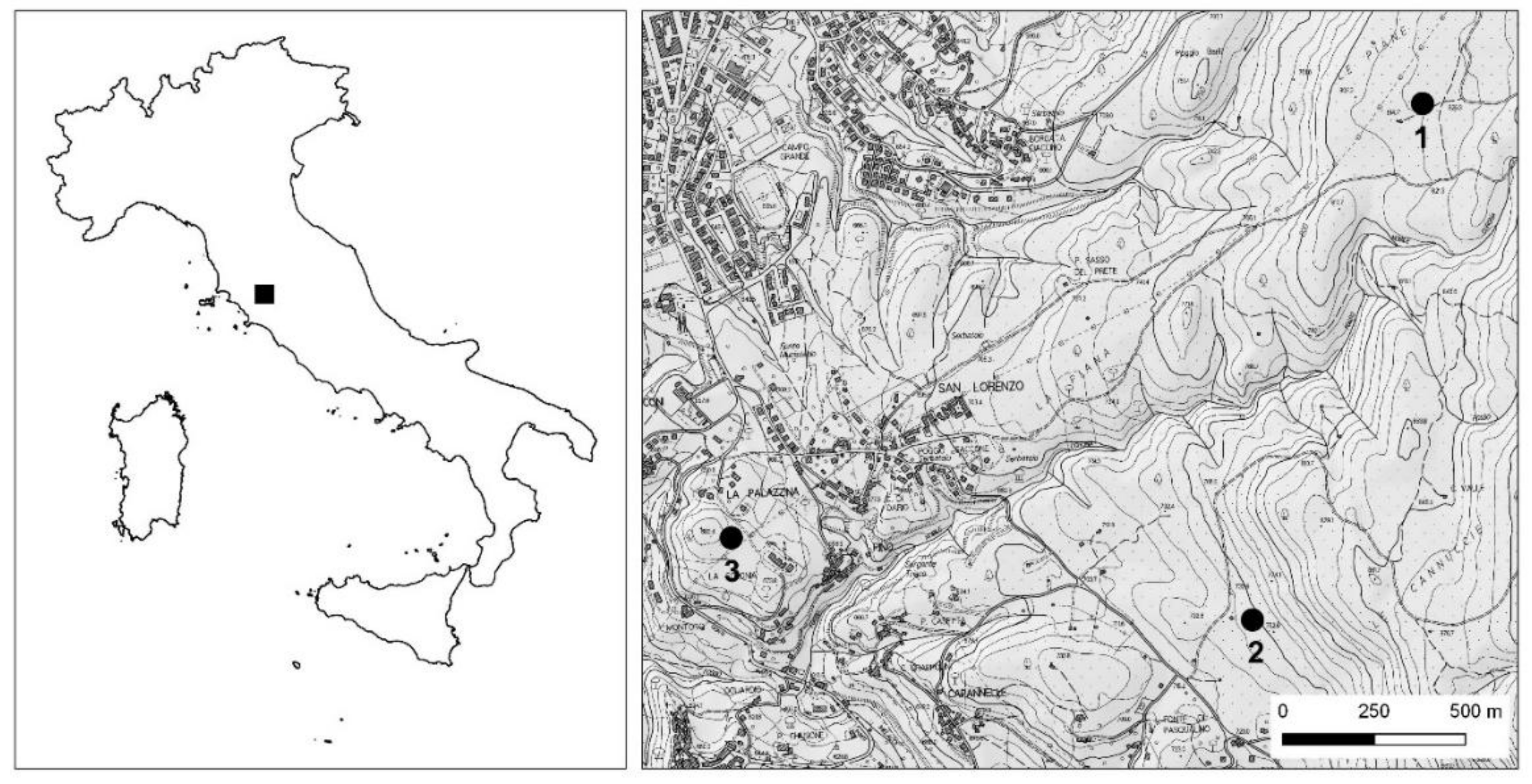
2.1. Study Area

The study was carried out in Mount Amiata, in the southern Tuscany region (Central Italy). Three pure sweet chestnut (Castanea sativa Mill.) stands, cultivated for fruit production, were identified in the area, hereinafter referred to as Area 1, Area 2, and Area 3 (Figure 1). In the region, the climate is Mediterranean, with rainfall of 919 mm yr−1 at Castel del Piano meteorological station (data 1961–1990), with a minimum in July and a maximum in November. The mean daily temperature over the year is 12.7 °C. Elevation ranges between 820 m a.s.l. in Area 1 and 680 m a.s.l. in Area 3. Area 1 and Area 3 are almost flat, while Area 2 is characterized by a slight slope (about 25%). The average tree density in the three areas (with DBH > 5 cm) is 110 trees ha−1.

2.2. Hand-Held Mobile Laser Scanning

We used the ZEB1 instrument as HMLS. The ZEB1 consists of a 3D laser scanner and an IMU, both mounted on top of a spring, which is itself located on a hand grip [32]. While the user walks through the forest, the scanner on the head of ZEB1 swings back and forth creating a 3D scanning field with data being captured at the speed of movement. Instead of using GNSS, it utilizes technology taken from the robotics community, simultaneous localization and mapping (SLAM), which is an algorithm that locates the scanner in an unknown environment and allows it to register the whole 3D point cloud, relying on both the IMU data and feature detection algorithms [30]. The reported operative laser range outdoors is 15–20 m, with a scan ranging noise of ±30 mm [34]. The main technical specifications of the instrument are reported in Table 1. A complete description of the instrument can be found in Giannetti et al. [33,35].

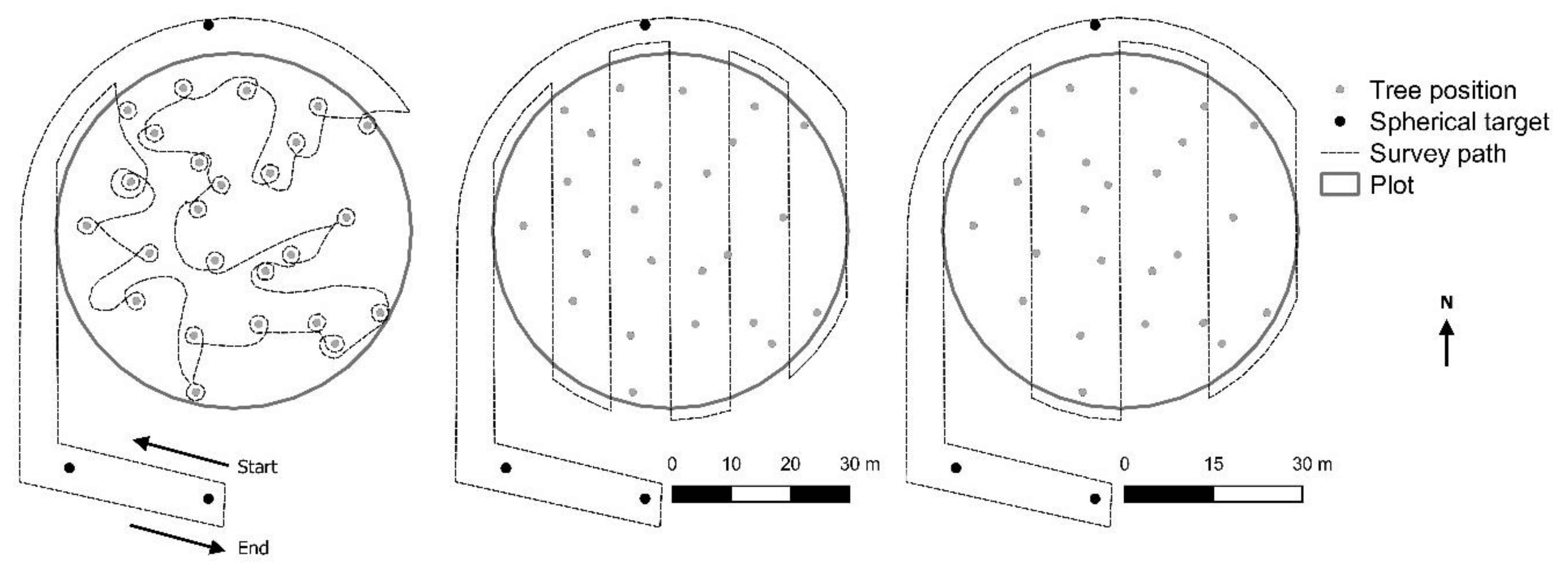
2.3. Hand-Held Mobile Laser Scanning Data Collection and Pre-Processing

Data acquisition was carried out on November 2016. In each area, the laser scanning data was collected within one circular plot with a radius of 30 m (0.28 ha).
Three spherical targets with a diameter of 14 cm were mounted on top of poles 1.5 m long and fixed on the ground around the plots to georeference the point cloud in post-processing. The coordinates of the spherical targets were acquired using the GNSS receiver Trimble Geo 7X. The post-processed coordinates revealed standard deviations for x, y, and z lower than 1, 1 and 2 cm, respectively.
To assess the influence of scan density on accuracy estimation, three different survey paths were considered (Figure 2). The first scan (D0) was performed by a person walking with ZEB1 HMLS around each tree, to avoid the effects of shadow zones and to obtain the highest scan density. The second and third scans were acquired by the same user walking back and forth along straight lines (obstacles were avoided) drawn at a distance of 10 m (D10) and 15 m (D15) from each other, respectively. For scans D10 and D15, the alignments were traced on the ground using poles and a surveyor’s cross. Each scan started and ended (i.e., the instrument was switched on and off) at a point fixed outside the plot to ensure a closed loop, as required when the SLAM algorithm is used. The time needed to perform each scan was recorded too.
The raw ZEB1 HMLS data were pre-processed on-line to obtain point clouds using the GeoSLAM procedure, which uses the SLAM algorithm. The pre-processing on-line procedure is subject to charges [33,34]. The charge costs depend on the length of the scan walking path, and the density of the scan point and can range between 0.05 and 0.15 €/m [34,35]. The cost of the on-line procedure for data pre-processing is reported in Table 2. The GeoSLAM procedure takes into account that the same objects are viewed from multiple directions as the system moves through the environment, and measurements to these objects are then used to calculate positions [29]. The SLAM algorithm processes IMU and laser data from the ZEB1 HMLS to locate the scanner in an unknown environment and to register the whole 3D point cloud without the need for GNSS [30,32]. More details on the SLAM algorithm can be found on-line at https://geoslam.com/slam/.
Once the 3D point cloud was obtained, we used the spherical targets to rotate and translate the cloud from the local coordinate system to the WGS84 UTM32N geographic coordinate system. CloudCompare software (CloudCompare version 2.9, 2017, www.cloudcompare.org) was used to automatically detect the spherical targets in the cloud and to assign the reference coordinate systems. The RMSE of roto-translation was approximately 4 cm.

2.4. Extraction of Single-Tree Attributes from the Point Clouds

The extraction of the single-tree attributes from the point clouds was done automatically with Computree software (Computree group, France, http://computree.onf.fr), which is an open source processing platform. Computree generated a digital terrain model at plot level and provided tools for automatic stem detection, DBH, and height estimation of each detected tree [30,36]. We used Computree to segment the point clouds into single-tree point clouds and to extract the single-tree attributes related to height (TH and CBH), DBH, and TP. The procedure to extract single-tree attributes was the same as that reported by Giannetti et al. [33].

2.5. Reference Data

The single-tree attributes extracted from the D0 scan (i.e., the scan performed walking around each tree) were assumed as error free here and used as reference data to evaluate the estimates produced on the basis of D10 and D15 scans.
The number of trees detected with the D0 scan in Area 1, Area 2, and Area 3 was 37, 25, and 36, respectively. Figure 3 shows the box-plot of the single-tree attributes related to DBH, TH, and CBH. The mean DBH was 44, 63, and 48 cm in Area 1, Area 2, and Area 3, respectively. Area 3 had a standard deviation of diameters higher than Area 1 and Area 2. The mean value of TH was 12 m in Area 1, 10 m in Area 2, and 8 m in Area 3. For all areas, mean CBH varied between 2 and 3 m.

2.6. Accuracy Assessment
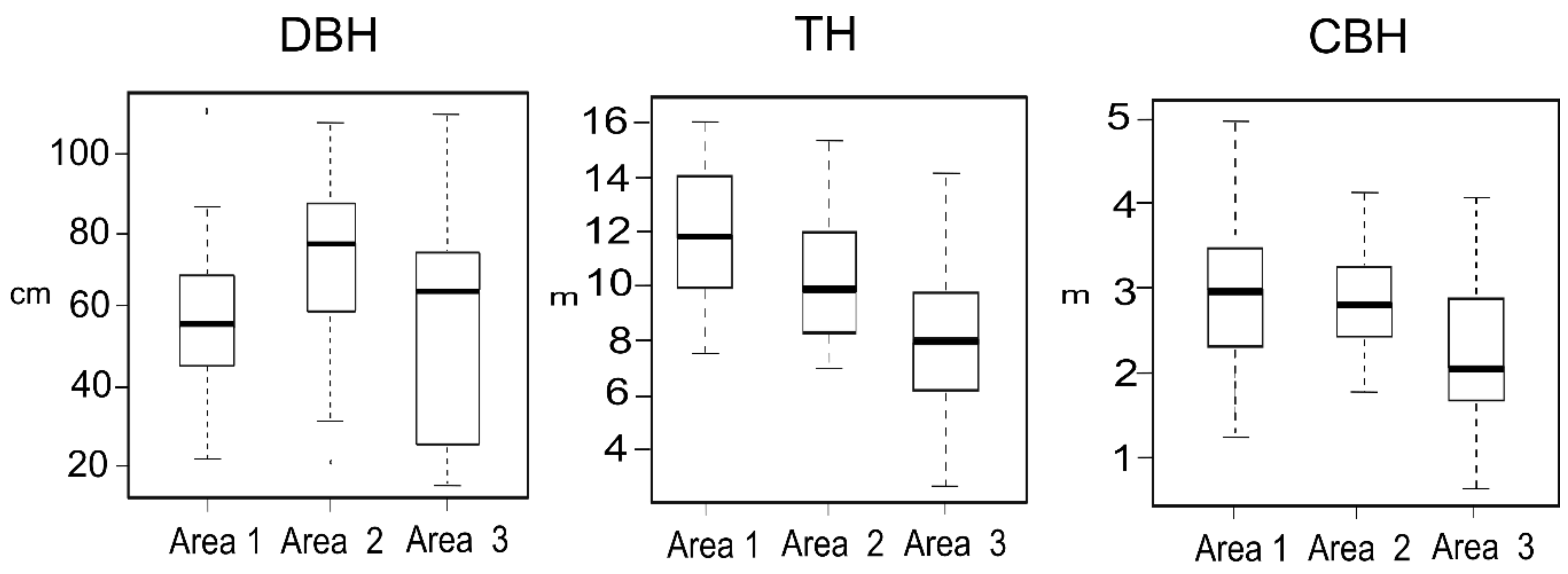
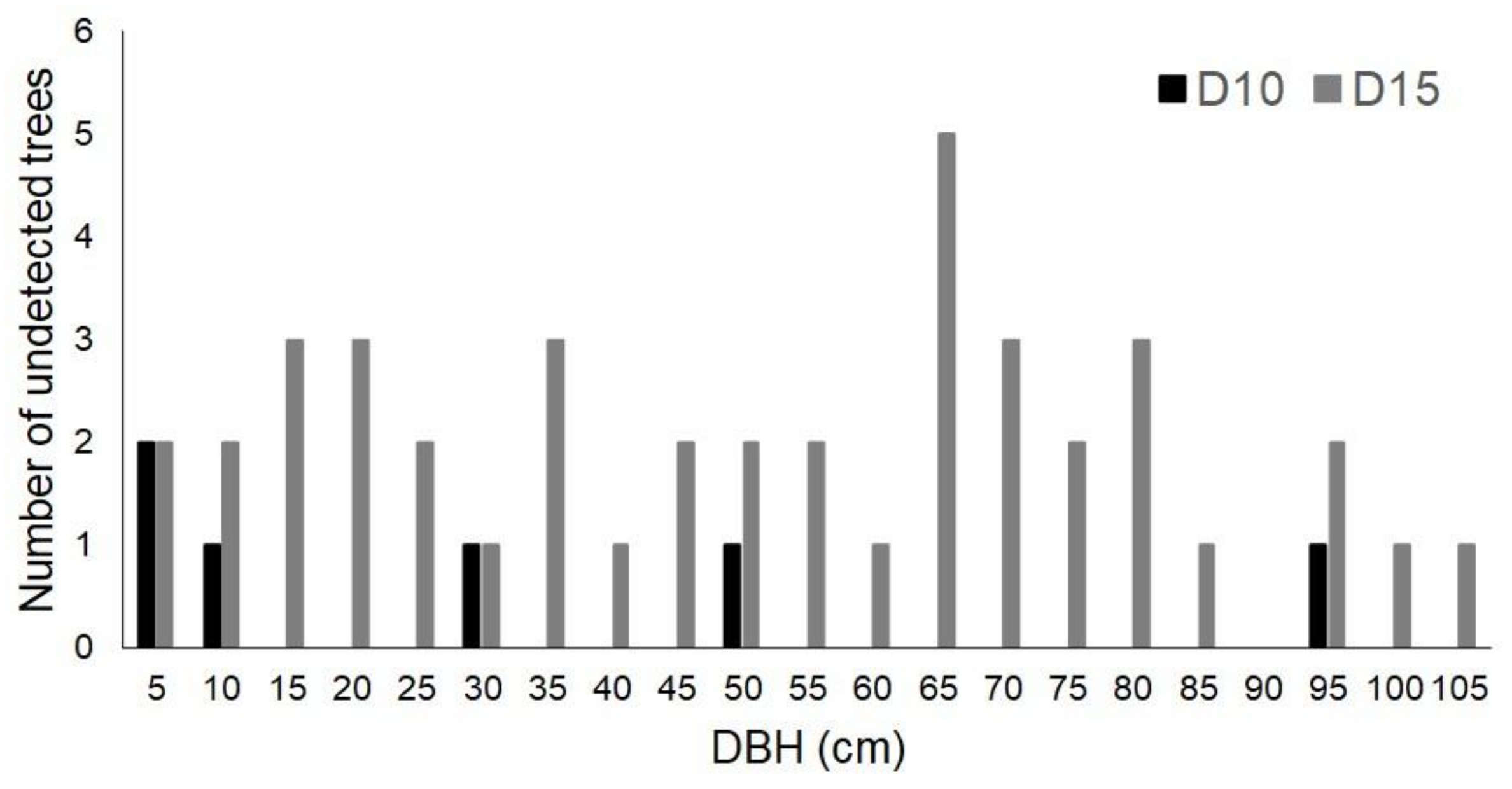
The single-trees attributes estimated by the D10 and D15 scans were compared with single-tree attributes obtained by the D0 scan.
To assess the accuracy of TP, DBH, TH, and CBH, we calculated the coefficient of determination (R2), the root mean square error (RMSE), the relative root mean square error (RMSE%), and bias as follows:
R M S E =   i = 1 n ( X o i X S i ) 2 n
R M S E   % = RMSE x ¯
b i a s =   i = 1 n ( X o i X S i ) n
where n is the number of trees resulting from the D0 scan, Xo is the value of the tree attribute computed in the D0 scan, Xs is the estimated value of the attribute for each i-th tree, and x ¯ is the mean value of the tree attribute computed in the D0 scan.
The number of trees estimated by the D10 and D15 scans was compared with the number of trees detected by the D0 scan; omission (i.e., stems that were detected in the D0 scan, but not in the D10 and D15 scans) and commission (i.e., stems that were undetected in the D0 scan, but were in the D10 and D15 scans) differences were computed. For omission errors, the size of the DBH of undetected trees was evaluated.

3. Results

The time spent to collect and elaborate the ZEB1 HMLS data and the cost related to the on-line pre-processing of point cloud divided by study areas and by path scans (i.e., D0, D10, and D15) are reported in Table 2. The cost of pre-processing ranged between 0.06 and 0.10 €/m. In detail, at plot level, we found differences in time and costs of data pre-processing between the D0 and the other two path scans. An average saving of total time of 10 min was observed between D10 and D0 scans, while a saving of 26 min was observed between D15 and D0 scans (Table 2). Moreover, for the pre-processing phase, an average saving of €14 was observed between D10 and D0 scans and €39 between D15 and D0 scans (Table 2).
Using the D0 scan as reference data, 98 trees were detected across all areas, with min/max DBH being 6 and 103 cm, respectively. Using the D10 scan data, 92 trees were estimated in the three areas, with DBH estimates in the range between 8 and 109 cm. Using the D15 scan data, the number of trees estimated in the three areas was 56 trees, with min/max DHB estimates between 8 and 107 cm, respectively. The omission difference across all areas compared to the reference data was 6% and 43%, respectively, for the D10 scan and the D15 scan (Table 3). Commission error was not found. The distribution of the DBH of undetected trees is reported in Figure 4. The map of the single-tree position is shown in Figure 5.
The accuracy of TP is reported in Table 4. The coefficient of determination for x and y coordinates was close to 1 for both the D10 and D15 scans. The RMSE and bias across all the three areas were 0.091 and −0.001 m for the D10 scan, respectively, and 0.139 m and −0.003 m for the D15 scan, respectively.
Table 5 shows the accuracy of the single-tree attributes (DBH, TH, and CBH) estimated by D10 and D15 scans. For the DBH, the coefficient of determination across all three areas was higher than 0.98, revealing a good fit between the D10 and the D15 scans and the reference data. Similar results are provided by RMSE%, which was lower than 6% for both scans. For TH, the coefficient of determination across the areas was higher than 0.94, with an RMSE% lower than 8% for the D10 and D15 scans. For CBH, the coefficient of determination was 0.91 and 0.87 and the RMSE% was 11% and 18% for the D10 and D15 scans, respectively.

4. Discussion

In this study we evaluated the performance of ZEB1 HMLS to assess single-tree attributes in pure sweet chestnut stands cultivated for fruit production. Two different survey paths (D10 and D15 scans) for data collection were tested to investigate the influence of scan density on estimation accuracies and acquisition costs. Scanning every tree by walking around the stem avoided the occlusion effect and allowed us to obtain the reference data (D0 scan) for the assessment.
TP was assessed with high accuracy across all the study areas, with slightly better results provided by the D10 scan (Table 4). The RMSE was 0.09 m for the D10 scan and 0.14 m for the D15 scan, and the bias was −0.001 m for the D10 scan and −0.003 m for the D15 scan. For TP, using the ZEB1 HMLS, Giannetti et al. [33] obtained an RMSE of 0.09 m and a bias of 0.021 m.
The DBH assessment provided good results with both scan densities. The RMSE was 2.5 cm and 2.9 cm and the bias was −0.22 cm and 0.14 cm for the D10 and D15 scans, respectively. However, the D10 scan resulted in a slightly lower RMSE% compared to the D15 scan (Table 5). These results are similar to those reported for ZEB1 HMLS by Ryding et al. [29] (RMSE = 2.9 cm and bias = 0.30 cm), Bauwens et al. [30] (RMSE = 1.11 cm and bias = −0.08 cm), Giannetti et al. [33] (RMSE = 1.28 cm and bias = −0.38 cm), and Oveland et al. [25] (RMSE = 3.1 cm and bias = 0.3 cm).
For TH, the RMSE and bias were 0.67 m and 0.168 m for the D10 scan, which had slightly better performances compared to the D15 scan (Table 5). Our results for TH are better than those reported by Giannetti et al. [33] (RMSE = 2.15 m and bias = −4.61 m) who tested the ZEB1 HMLS in a Mediterranean multi-layered forest stand. In fact, it is known that the direct measure of tree heights by terrestrial laser scanner is limited by the laser range when the range is similar to tree heights and/or by point occlusion within the point cloud due to dense vegetation layers [18,37]. For ZEB1 HMLS, Bauwens et al. [30] found that most of the laser signal does not penetrate 15–20 m in height. However, in the case of multi-layered forest stands, better results for the estimation of TH by HMLS can be obtained by integrating terrestrial and airborne laser scanning data [33]. In our case studies, tree heights (Figure 3) were slightly smaller than the laser range (15–20 m) and no dense vegetation layers were present.
CBH was estimated with an RMSE% higher than the one obtained for DBH and TH. However, the D10 scan was able to provide assessment slightly better than the D15 scan (Table 5), with an RMSE of 0.30 m and a bias of −0.14 m. The complexity in estimating the CBH is also reported by Giannetti et al. [33] who obtained a bias of 1.67 m, an RMSE of 1.91 m, and an RMSE% of 40% due to the difficulties of recognizing dead branches on the bases of the ZEB1 HMLS cloud.
The assessment of the number of trees was influenced by scan density more than the other single-tree attributes. The D10 scan was not able to detect six out 96 trees across all the three areas, with an omission difference of 6%. Similar results were obtained by Ryding et al. [29] who reported an omission difference of 9%. Using the D15 scan data set, 42 trees were undetected, with an omission error of 43%. Half of the undetected trees in the D10 scan had a DBH in the range between 6 and 8 cm. For the D15 scan, 90% of undetected trees had a DBH higher than 10 cm (Figure 4). Other studies reported that in the case of stems with a DBH < 10 cm, the small size of the target resulted in fewer point returns, which hindered the tree detection process in the point cloud [29]. For the ZEB1 HMLS, the manufacturer reports that the laser range outdoors is 15–20 m. Our study shows that collecting data with ZEB1 HMLS with the user walking with the instrument along straight lines 15 m distant from each other provides a point cloud unsuitable to obtain satisfying results for tree detection. With this scan density, we were not able to model several large stems in the cloud due to the few point returns available. Occlusion effects might have influenced the results of the D15 scan.
Regarding the time needed to collect the ZEB1 HMLS data (Table 2), one surveyor was able to scan a plot of 2827 m2 with an average time of 13.6 min (48 min ha−1) and 10.3 min (38 min ha−1) for the D10 and D15 scans, respectively. In a previous study, conducted in the same three areas using conventional manual measurement instruments (e.g., calliper and hypsometer), the same single-tree attributes were collected by two surveyors with an average survey time of 100 min ha−1 [38]. The survey time reported by other authors [29,30,33], who collected the ZEB1 HMLS data in more complex forest structures with respect to our study areas, are in the range between 130 and 200 min ha−1. Analyzing the cost of the data pre-processing, and the total time needed to acquire and extract single-tree parameters from each plot cloud, we found that following the D10 path there is an average decrease in cost of €14 for data pre-processing and an average decrease of 37 min for data acquisition, analysis, and single-tree attribute estimations (Table 2). From these results, we can affirm that the use of D10, which allows the acquisition of single-tree data that are in line with D0 and previous studies [25,29,30,33], could be efficient in terms of balance between accuracy, cost, and time. In fact, if we assume the collection of 30 field plots with a size of 1256 m2, which is usual for forest management plans of about 250 ha chestnut stands, our results (Table 2) show that by using D0 we can estimate approximately 125 h of work (field work, point clouds analysis, and single-tree attribute estimation), while with D10 the workload decrease to 106.5 h. Moreover, we can estimate a decrease of the cost of pre-processing from €2580 to €2160 due to the reduction of the walking path length [35]. However, it is worth of noting that the structure of the sweet chestnut stands cultivated for fruit production, which are characterized by a relatively low tree density, large stems, and without an understory layer, has simplified our study in terms of time needed to collect the data. Other studies conducted in more complex forest stands underlined how the workload necessary for point cloud segmentation and single-tree attribute extraction may require more time compared to what we found in this study. For example, Giannetti et al. [33] report a workload of about 50 man-days for coding and optimizing the procedures for point cloud segmentation and single-tree attribute extraction in a Mediterranean forest type dominated by coniferous and evergreen broadleaves, due to the high level of intersection between tree crowns and the complexity of the vertical structure (dominated trees under dominant trees). However, forest conditions similar to the stand structures examined in our study can be found in Italy in other forest types, such as in mature even-aged high forests dominated by Fagus sylvatica L., Quercus sp. or Pinus pinea L.
The knowledge of single-tree attributes like those considered in this work is clearly of interest in the framework of forest inventories, for instance to assess the number of trees, to estimate the basal area, or to assess tree volume or biomass (e.g., using double entry equations), which can be used as a proxy to estimate the amount of carbon stocked by a forest. However, also in sweet chestnut stands cultivated for fruit production, the estimation of single-tree attributes can be of interest for forest owners and managers. For example, to assess crown length as the algebraical subtraction of the crown base height from tree height, which can be used to evaluate the cost of pruning—one of the most common silvicultural activities carried out in this forest type [39]—or to estimate the amount of chestnuts production based on tables that take into account the diameter of the trees [40].

5. Conclusions

HMLS systems have been recognized as promising tools to collect the 3D structure of a forest, with potential practical application in forest inventory and forest monitoring. With HMLS, accurate information on tree position and DBH can be obtained with lower survey times than those required by static terrestrial laser scanners and conventional field measurements. However, the accuracy of the estimates based on HMLS is influenced by the survey path followed by the user during data acquisition, thus new solutions to optimize the walking scan line should be tested.
Based on the results obtained in our work, which was carried out with ZEB1 HMLS in sweet chestnut stands with simplified forest structures, four main conclusions can be drawn from the study. Firstly, walking around each tree (D0 scan) improves the detection of the trees with small diameters (DBH < 10 cm), but this solution is not feasible in dense and complex forest structures and requires high acquisition times. Secondly, walking back and forth along straight lines drawn at a distance of 10 m (D10) from each other provides sufficient data to assess single-tree attributes, such as tree position, DBH, tree height, and crown base height, with results similar to those obtained walking around each tree; this survey scheme is simple to put into practice and produced an omission error smaller than 10%. Thirdly, survey schemes based on straight lines drawn at a distance higher than 10 m from each other are not recommended; using 15 m distance between the walking scan lines, more than 40% of the trees were undetected, independent of the stem size. Lastly, the D10 scan enables the right balance between time of acquisition and extraction of accurate results reducing the cost of pre-processing data.
These findings can help in planning future HMLS surveys in the context of forest inventory applications. However, because our study is based on a specific type of HMLS (ZEB1), which has been evaluated in a simplified forest structure using a specific survey path (straight lines drawn with different spacing), further studies are needed to test the performances of other possible survey schemes and other types of HMLS instruments in different forest types and more complex forest structures.

Author Contributions

Conceptualization, G.C. and D.T.; data curation, B.D.P. and F.G.; formal analysis, B.D.P. and F.G.; funding acquisition, D.T.; methodology, F.G., G.C., and D.T.; supervision, G.C. and D.T.; writing—original draft, B.D.P.

Funding

This research was funded by the LIFE program in the framework of the project “FRESh LIFE—demonstrating remote sensing integration in sustainable forest management” (LIFE14 ENV/IT/000414).

Acknowledgments

We thank the Unione dei Comuni Amiata Grossetana and the Association for Valorizzazione della Castagna del Monte Amiata for their support for the research activity execution. Thanks to Alberto Maltoni for his comments on the discussion section. The authors wish to thank the Co-Chief Managing Editor, Chenxi Wei, and the two anonymous reviewers for their positive contribution to improving the manuscript.

Conflicts of Interest

The authors declare no conflicts of interest.

References

  1. Næsset, E.; Gobakken, T.; Holmgren, J.; Hyyppä, H.; Hyyppä, J.; Maltamo, M.; Nilsson, M.; Olsson, H.; Persson, Å.; Söderman, U. Laser scanning of forest resources: the nordic experience. Scand. J. For. Res. 2004, 19, 482–499. [Google Scholar] [CrossRef]
  2. Tomppo, E.; Olsson, H.; Ståhl, G.; Nilsson, M.; Hagner, O.; Katila, M. Combining national forest inventory field plots and remote sensing data for forest databases. Remote Sens. Environ. 2008, 112, 1982–1999. [Google Scholar] [CrossRef]
  3. Corona, P.; Chirici, G.; McRoberts, R.E.; Winter, S.; Barbati, A. Contribution of large-scale forest inventories to biodiversity assessment and monitoring. For. Ecol. Manage. 2011, 262, 2061–2069. [Google Scholar] [CrossRef] [Green Version]
  4. Kangas, A.; Astrup, R.; Breidenbach, J.; Fridman, J.; Gobakken, T.; Korhonen, K.T.; Maltamo, M.; Nilsson, M.; Nord-Larsen, T.; Næsset, E.; et al. Remote sensing and forest inventories in Nordic countries – roadmap for the future. Scand. J. For. Res. 2018, 7581, 1–16. [Google Scholar] [CrossRef]
  5. Liang, X.; Kankare, V.; Hyyppä, J.; Wang, Y.; Kukko, A.; Haggrén, H.; Yu, X.; Kaartinen, H.; Jaakkola, A.; Guan, F.; et al. Terrestrial laser scanning in forest inventories. ISPRS J. Photogramm. 2016, 115, 63–77. [Google Scholar] [CrossRef] [Green Version]
  6. Brosofske, K.D.; Froese, R.E.; Falkowski, M.J.; Banskota, A. A review of methods for mapping and prediction of inventory attributes for operational forest management. For. Sci. 2014, 60, 733–756. [Google Scholar] [CrossRef]
  7. Rahlf, J.; Breidenbach, J.; Solberg, S.; Næsset, E.; Astrup, R. Comparison of four types of 3D data for timber volume estimation. Remote Sens. Environ. 2014, 155, 325–333. [Google Scholar] [CrossRef]
  8. Miller, J.; Morgenroth, J.; Gomez, C. 3D modelling of individual trees using a handheld camera: Accuracy of height, diameter and volume estimates. Urban For. Urban Green. 2015, 14, 932–940. [Google Scholar] [CrossRef]
  9. Solberg, S.; Naesset, E.; Bollandsas, O.M. Single Tree Segmentation Using Airborne Laser Scanner Data in a Structurally Heterogeneous Spruce Forest. Photogramm. Eng. Remote Sens. 2006, 72, 1369–1378. [Google Scholar] [CrossRef]
  10. Wulder, M.A.; Bater, C.W.; Coops, N.C.; Hilker, T.; White, J. The role of LiDAR in sustainable forest management. For. Chron. 2008, 84, 807–826. [Google Scholar] [CrossRef] [Green Version]
  11. Hyyppä, J.; Kelle, O.; Lehikoinen, M.; Inkinen, M. A segmentation-based method to retrieve stem volume estimates from 3-D tree height models produced by laser scanners. IEEE Trans. Geosci. Remote Sens. 2001, 39, 969–975. [Google Scholar] [CrossRef]
  12. Yang, B.; Dai, W.; Dong, Z.; Liu, Y. Automatic Forest Mapping at Individual Tree Levels from Terrestrial Laser Scanning Point Clouds with a Hierarchical Minimum Cut Method. Remote Sens. 2016, 8, 372. [Google Scholar] [CrossRef]
  13. Bottalico, F.; Travaglini, D.; Chirici, G.; Marchetti, M.; Marchi, E.; Nocentini, S.; Corona, P. Classifying silvicultural systems (coppices vs. high forests) in mediterranean oak forests by airborne laser scanning data. Eur. J. Remote Sens. 2014, 47, 437–460. [Google Scholar] [CrossRef]
  14. Bottalico, F.; Chirici, G.; Giannini, R.; Mele, S.; Mura, M.; Puxeddu, M.; McRoberts, R.E.; Valbuena, R.; Travaglini, D. Modeling Mediterranean forest structure using airborne laser scanning data. Int. J. Appl. Earth Obs. Geoinf. 2017, 57, 145–153. [Google Scholar] [CrossRef]
  15. Mura, M.; McRoberts, R.E.; Chirici, G.; Marchetti, M. Estimating and mapping forest structural diversity using airborne laser scanning data. Remote Sens. Environ. 2015, 170, 133–142. [Google Scholar] [CrossRef]
  16. Mura, M.; McRoberts, R.E.; Chirici, G.; Marchetti, M. Statistical inference for forest structural diversity indices using airborne laser scanning data and the k-Nearest Neighbors technique. Remote Sens. Environ. 2016, 186, 678–686. [Google Scholar] [CrossRef]
  17. Kankare, V.; Liang, X.; Vastaranta, M.; Yu, X.; Holopainen, M.; Hyyppä, J. Diameter distribution estimation with laser scanning based multisource single tree inventory. ISPRS J. Photogramm. 2015, 108, 161–171. [Google Scholar] [CrossRef]
  18. Chirici, G.; McRoberts, R.E.; Fattorini, L.; Mura, M.; Marchetti, M. Comparing echo-based and canopy height model-based metrics for enhancing estimation of forest aboveground biomass in a model-assisted framework. Remote Sens. Environ. 2016, 174, 1–9. [Google Scholar] [CrossRef]
  19. Talbot, B.; Pierzchała, M.; Astrup, R. Applications of Remote and Proximal Sensing for Improved Precision in Forest Operations. Croat. J. For. Eng. 2016, 38, 327–336. [Google Scholar]
  20. Holopainena, M.; Kankarea, V.; Vastarantaa, M.; Liangb, X.; Linb, Y.; Vaajac, M.; Yub, X. Tree mapping using airborne, terrestrial and mobile laser scanning – A case study in a heterogeneous urban forest. Urban For. Urban Green 2013, 12, 546–553. [Google Scholar] [CrossRef]
  21. Zlot, R.; Bosse, M.; Greenop, K.; Jarzab, Z.; Juckes, E.; Roberts, J. Efficiently capturing large, complex cultural heritage sites with a handheld mobile 3D laser mapping system. J. Cult. Herit. 2014, 15, 670–678. [Google Scholar] [CrossRef]
  22. Hopkinson, C.; Chasmer, L.; Young-Pow, C.; Treitz, P. Assessing forest metrics with a ground-based scanning LiDAR. Can. J. Remote Sens. 2004, 34, 573–583. [Google Scholar] [CrossRef]
  23. Thies, M.; Pfeifer, N.; Winterhalder, D.; Gorte, B.G.H. Three-dimensional reconstruction of stems for assessment of taper, sweep, and lean based on laser scanning of standing trees. Scand. J. For. Res. 2004, 19, 571–581. [Google Scholar] [CrossRef]
  24. Maas, H.-G.; Bienert, A.; Scheller, S.; Keane, E. Automatic forest inventory parameter determination from terrestrial laser scanner data. Int. J. Remote Sens. 2008, 29, 1579–1593. [Google Scholar] [CrossRef]
  25. Oveland, I.; Hauglin, M.; Giannetti, F.; Kjørsvik, N.S.; Gobakken, T. Comparing three different ground based laser scanning methods for tree stem detection. Remote Sens. 2018, 10, 538. [Google Scholar] [CrossRef]
  26. Dassot, M.; Constant, T.; Fournier, M. The use of terrestrial LiDAR technology in forest science: Application fields, benefits and challenges. Ann. For. Sci. 2011, 68, 959–974. [Google Scholar] [CrossRef]
  27. Kuronen, M.; Henttonen, H.M.; Myllymäki, M. Correcting for nondetection in estimating forest characteristics from single-scan terrestrial laser measurements. Can. J. For. Res. 2019, 49, 96–103. [Google Scholar] [CrossRef]
  28. Liang, X.; Kukko, A.; Kaartinen, H. Possibilities of a personal laser scanning system for forest mapping and ecosystem services. Sensors 2014, 14, 1228–1248. [Google Scholar] [CrossRef]
  29. Ryding, J.; Williams, E.; Smith, M.; Eichhorn, M. Assessing handheld mobile laser scanners for forest surveys. Remote Sens. 2015, 7, 1095–1111. [Google Scholar] [CrossRef]
  30. Bauwens, S.; Bartholomeus, H.; Calders, K.; Lejeune, P. Forest Inventory with Terrestrial LiDAR: A Comparison of Static and Hand-Held Mobile Laser Scanning. Forests 2016, 7, 127. [Google Scholar] [CrossRef]
  31. Forsman, M.; Holmgren, J.; Olofsson, K. Tree Stem Diameter Estimation from Mobile Laser Scanning Using Line-Wise Intensity-Based Clustering. Forests 2016, 7, 206. [Google Scholar] [CrossRef]
  32. Bosse, M.; Zlot, R.; Flick, P. Zebedee: Design of a spring-mounted 3-d range sensor with application to mobile mapping. IEEE Trans. Robot 2012, 28, 1104–1119. [Google Scholar] [CrossRef]
  33. Giannetti, F.; Puletti, N.; Quatrini, V.; Travaglini, D.; Bottalico, F.; Corona, P.; Chirici, G. Integrating terrestrial and airborne laser scanning for the assessment of single tree attributes in Mediterranean forest stands. Eur. J. Remote Sens. 2018, 51, 795–807. [Google Scholar] [CrossRef]
  34. GEOSLAM. User Manual; GeoSLAM Ltd.: Den Haag, The Nederland, 2017. [Google Scholar]
  35. Giannetti, F.; Chirici, G.; Travaglini, D.; Bottalico, F.; Marchi, E.; Cambi, M. Assessment of Soil Disturbance Caused by Forest Operations by Means of Portable Laser Scanner and Soil Physical Parameters. Soil Sci. Soc. Am. J. 2017, 81, 1577–1585. [Google Scholar] [CrossRef]
  36. Hackenberg, J.; Spiecker, H.; Calders, K.; Disney, M.; Raumonen, P. SimpleTree–An efficient open source tool to build tree models from TLS Clouds. Forests 2015, 6, 4245–4294. [Google Scholar] [CrossRef]
  37. Liang, X.; Hyyppä, J. Automatic stem mapping by merging several terrestrial laser scans at the feature and decision levels. Sensors 2013, 13, 1614–1634. [Google Scholar] [CrossRef] [PubMed]
  38. Bertini, R.; Faini, A.; Montaghi, A.; Puletti, N.; Travaglini, D. (In Italian) Methodology for the census and mapping of chestnut forests. In III Congresso Nazionale di Selvicoltura, Taormina, Italy, 16-19 ottobre 2008, Accademia Italiana di Scienze Forestali, vol. Atti del III Congresso Nazionale di Selvicoltura per il miglioramento e la conservazione dei boschi italiani, 16-19 ottobre 2008 – Taormina (Messina); Accademia Italiana di Scienze Forestali: Florence, Italy, 2009; Volume 3, pp. 1455–1461. ISBN 9788887553161. [Google Scholar]
  39. Maltoni, A.; Mariotti, B.; Jacobs, D.F.; Tani, A. Pruning methods to restore Castanea sativa stands attacked by Dryocosmus kuriphilus. New For. 2012, 43, 869–885. [Google Scholar] [CrossRef]
  40. Piccioli, L. Monografia del Castagno (In Italian), 2nd ed.; Stab. Tipo-Litografico G. Spinelli & C.: Florence, Italy, 1922; p. 397. [Google Scholar]
Figure 1. Location of the three study areas.
Forests 10 00277 g001
Figure 2. Survey paths used for the scans with HMLS (ZEB1): walking with the instrument around each tree (D0 scan, left), and walking back and forth along straight lines drawn at a distance of 10 m (D10 scan, center) and 15 m (D15 scan, right) from each other.
Forests 10 00277 g002
Figure 3. Boxplot with resulting values for diameter at breast height (DBH), tree height (TH) and crown base height (CBH) of the reference data (D0 scan).
Forests 10 00277 g003
Figure 4. Stem number–diameter distribution of undetected trees by D10 and D15 scans. Data for all three areas are reported.
Forests 10 00277 g004
Figure 5. Single-tree position in the three areas estimated with D10 and D15 scans vs the reference data (D0 scan).
Forests 10 00277 g005
Table 1. Technical specifications of the hand-held mobile laser scanning (HMLS) (ZEB1).
FeatureDescription
Laser scanner sensor905-nm wavelength and a beam divergence of approximately 7 mrad.
WeightHand-held sensor, 0.7 kg.
Data logger in backpack, 3.6 kg.
Frequency of scanning43,200 points/s (40 lines/s with a laser pulse interval of 0.25°).
Field of view Horizontally 270°.
Vertically 120°.
Measurement error±30 mm at a range of 0.1 m to 10 m.
Table 2. Time and cost needed for HMLS (ZEB1) data acquisition and processing. Average time/ha column refers to the sum of scan time and extraction of single-tree data columns. Time is reported in minutes, length in meters, and costs in Euro.
Path Scan Length of Walking Path (m)Scan Time (min)Extraction of Single-Tree Data (min)Pre-Processing Cost (€)Average Time/ha (min/ha)
AreaAreaAreaArea
123123123123
D0956842828171513585653938976250
D10722721704151412494546727569213
D1562160259212118383133524841157
Table 3. Number of trees estimated with D10 and D15 scans vs the reference data (D0 scan).
AreaNumber of TreesOmission Difference (%)
D0D10D15D10D15
1373724035
2252512052
33630201744
All989256643
Table 4. Summary statistics of single-tree position estimated by D10 and D15 scans. Root mean square error (RMSE) and bias are reported in meters.
AreaRMSEBias
D10D15D10D15
10.0010.0050.000−0.001
20.1390.244−0.015−0.024
30.0970.1360.0090.007
All0.0910.139−0.001−0.003
Table 5. Summary statistics of single-tree attributes (DBH, TH, and CBH) estimated by D10 and D15 scans.
Single-Tree AttributeAreaR2RMSERMSE%Bias
D10D15D10D15D10D15D10D15
DBH (cm)10.9830.9810.7682.5440.0025.2400.001−0.100
20.9750.9793.9193.9936.2087.0280.3621.578
30.9950.9942.3812.5895.0325.445−0.981−0.430
All0.9910.9862.4512.9304.7755.864−0.2220.142
TH (m)10.9840.9450.5340.6444.5345.3590.2860.309
20.9130.9800.7040.2966.8933.0420.3080.163
30.8790.9290.9841.14311.54412.6390.2590.777
All0.9520.9430.6710.8146.5237.7810.1680.445
CBH (m)11.0000.9580.1980.2727.0249.762−0.015−0.209
20.9170.6600.2550.8048.77126.280−0.140−0.463
30.8620.9580.4740.45319.62518.217−0.298−0.302
All0.9150.8720.3020.49411.12618.016−0.135−0.297

