Modelling and Predicting the Growing Stock Volume in Small-Scale Plantation Forests of Tanzania Using Multi-Sensor Image Synergy

Abstract

Remotely sensed assisted forest inventory has emerged in the past decade as a robust and cost efficient method for generating accurate information on forest biophysical parameters. The launching and public access of ALOS PALSAR-2, Sentinel-1 (SAR), and Sentinel-2 together with the associated open-source software, has further increased the opportunity for application of remotely sensed data in forest inventories. In this study, we evaluated the ability of ALOS PALSAR-2, Sentinel-1 (SAR) and Sentinel-2 and their combinations to predict growing stock volume in small-scale forest plantations of Tanzania. The effects of two variable extraction approaches (i.e., centroid and weighted mean), seasonality (i.e., rainy and dry), and tree species on the prediction accuracy of growing stock volume when using each of the three remotely sensed data were also investigated. Statistical models relating growing stock volume and remotely sensed predictor variables at the plot-level were fitted using multiple linear regression. The models were evaluated using the k-fold cross validation and judged based on the relative root mean square error values (RMSEr). The results showed that: Sentinel-2 (RMSEr = 42.03% and pseudo − R² = 0.63) and the combination of Sentinel-1 and Sentinel-2 (RMSEr = 46.98% and pseudo − R² = 0.52), had better performance in predicting growing stock volume, as compared to Sentinel-1 (RMSEr = 59.48% and pseudo − R² = 0.18) alone. Models fitted with variables extracted from the weighted mean approach, turned out to have relatively lower RMSEr % values, as compared to centroid approaches. Sentinel-2 rainy season based models had slightly smaller RMSEr values, as compared to dry season based models. Dense time series (i.e., annual) data resulted to the models with relatively lower RMSEr values, as compared to seasonal based models when using variables extracted from the weighted mean approach. For the centroid approach there was no notable difference between the models fitted using dense time series versus rain season based predictor variables. Stratifications based on tree species resulted into lower RMSEr values for Pinus patula tree species, as compared to other tree species. Finally, our study concluded that combination of Sentinel-1&2 as well as the use Sentinel-2 alone can be considered for remote-sensing assisted forest inventory in the small-scale plantation forests of Tanzania. Further studies on the effect of field plot size, stratification and statistical methods on the prediction accuracy are recommended.

1. Introduction

Accurate estimates of forest attributes such as volume and biomass are important for supporting sustainable forest management strategies and for implementing climate change mitigation policies [1,2]. Traditionally, such attributes have been derived from field sample surveys based on a statistical sampling of the forest landscape being studied [3]. Recently, remote-sensing techniques like Airborne Laser Scanning (ALS) and high-resolution optical satellite images have been used in combination with field-based surveys to provide a synoptic view over large areas at different temporal and spatial scales. This has increased the efficiency of forest measurements compared with field-based methods [4]. However, limitations related to data availability, high cost and the volume [5,6] of commercial high-resolution remote-sensing data impede their operational forestry applications in low income countries. Thus, there is a need to develop cost-efficient and affordable methods, which provide successful forest volume and biomass estimates in various environments [7].

The amount of open access, medium to high-resolution optical satellite data available from global repositories has increased over the past decade. The Landsat archives were opened to the public in 2008 [8], the Advance Spaceborne Thermal Emission and reflection Radiometer (ASTER) archives were opened in 2014 and the Sentinel-2A and Sentinel-2B satellites have been operative since 2015 and 2017, respectively. The Sentinel-2 satellites provide important developments in spatial, temporal, and radiometric resolution to the globally available open-source optical image catalogue. On top of the increased availability of optical imagery, the Synthetic Aperture Radar (SAR) imagery has become open access. The European Space Agency (ESA) launched the Sentinel-1A and Sentinel-1B satellites in 2014 and 2016, both carrying dual-polarized C-band SAR sensor providing global imagery with 12 days of revisit time at the equator [9]. In addition, the Japanese Aerospace Exploration Agency (JAXA) distributes global mosaics of Advanced Land Observing Satellite (ALOS) dual-polarised L-Band SAR backscatter data yearly [10]. Altogether, open-access policy combined with the evolving processing capacity of cloud-computing environments have created new opportunities for multi-source data modeling in the field of forestry, which is vital in low income and data-scarce regions.

Optical satellite sensors have been widely used to estimate and model forest attributes, such as forest area and character [11,12], volume [13,14,15], and above ground biomass (AGB) See survey by [16] due to their sensitivity to vegetation response observed in multispectral bands. However, optical sensors are obstructed by atmospheric conditions and cloud cover, which reduces their potential operational use especially in cloudy prone areas. In contrast, SAR sensors can produce images independent of daylight or atmospheric conditions. The backscatter of the SAR sensor is a function of surface characteristics, depending on the band wavelength and polarization. In particular, L-band imagery is widely used to predict AGB and growing stock volume (GSV) because it can capture the branch and trunk structure [17,18,19]. Thus, combined use of optical and SAR sensor imagery can integrate the strengths and complement the limitations of different sensors over other methods [20,21,22].

To date, a number of studies have reported interesting results when combining optical and SAR imagery in forestry applications. For example, Torbick, et al. [23] found that a fusion of Landsat-8, PALSAR-2, and Sentinel-1 imagery efficiently captures the characteristics of various plantation species and the differences in planted and natural forests. Laurin, et al. [24] reported that integrating the Sentinel-2 imagery with SAR imagery in mapping AGB enables the investigation of seasonality, especially in deciduous forest via their distinct temporal response in optical time series. However, the estimations based on integrated datasets were suspect for AGB overestimation. On the other hand, Vafaei, et al. [25] found that using Sentinel-2 data alone can provide reasonable estimates on AGB, and the estimates are improved when integrated with SAR imagery. These studies have shown that integrated and multi-temporal use of optical and SAR imagery can provide improved and credible estimates on forest attributes. Still further research is needed to evaluate the opportunities and limitations of applying multi-sensor integration in tropical cloud-prone regions and in small-scale plantation landscapes. As Sentinel-1 and Sentinel-2 missions are operational, providing synergetic data on optical and microwave spectrum with global coverage, open an opportunity for facilitating their operational applications in forest attribute monitoring [26], especially in the Global South where access to high-resolution satellite imagery and the availability of an intensive field inventory has been limited. Furthermore, as most of the recent studies are modelling AGB, more evidence is needed on how well these methods predict GSV. Spatially explicit information on GSV is vital for strategic forest management and can be used to estimate AGB and to support the REDD+ (reducing emissions from deforestation and forest degradation, and fostering conservation, sustainable management of forests, and enhancement of forest carbon stocks) processes [26,27].

In Tanzania, private industrial-scale forest plantations and non-industrial private forests (individual woodlots, farm trees, and out-growers schemes) have been growing rapidly in the past few decades, especially in the Southern Highlands region [28,29,30]. A large part of the GSV lies in the fragmented landscape of smallholder woodlots, where estimations on the productive area and yield have not been yet made. This information gap hinders the efficient decisions of forest managers, individual owners and investors, and it affects the credibility of regional and countrywide forest resources statistics, which are important for climate change mitigation policies and global forest resources initiatives of the Food and Agriculture Organization of the United Nations. Methodologies enabling scientific estimations of forest attributes in diverse landscape plantations, are needed as both government and private forests are expected to support the Tanzania’s industrial economy by providing wood raw materials to forest-based industries and by supplying other goods and services to communities [28,31].

The overreaching goal of this study is to evaluate the accuracy of GSV predictions based on Sentinel-1, Sentinel-2 images, and ALOS PALSAR-2 global mosaics, in a small-scale private plantation forest of Tanzania. Our aim is to develop various models by combining predictors derived from optical and microwave sensor images, and testing their performance in predicting GSV at the plot-level. The remote-sensing variables are extracted for each plot measurement via centroid and area weighted mean approaches to evaluate the sensitivity of the extraction method. Furthermore, we test the impact of seasonality, and post stratification of plantation species, in volume model performance. Our approach brings new insights in evaluating the best practice for estimating GSV using satellite-based remote-sensing techniques in a small-scale and heterogeneous plantation environment.

2. Materials and Methods

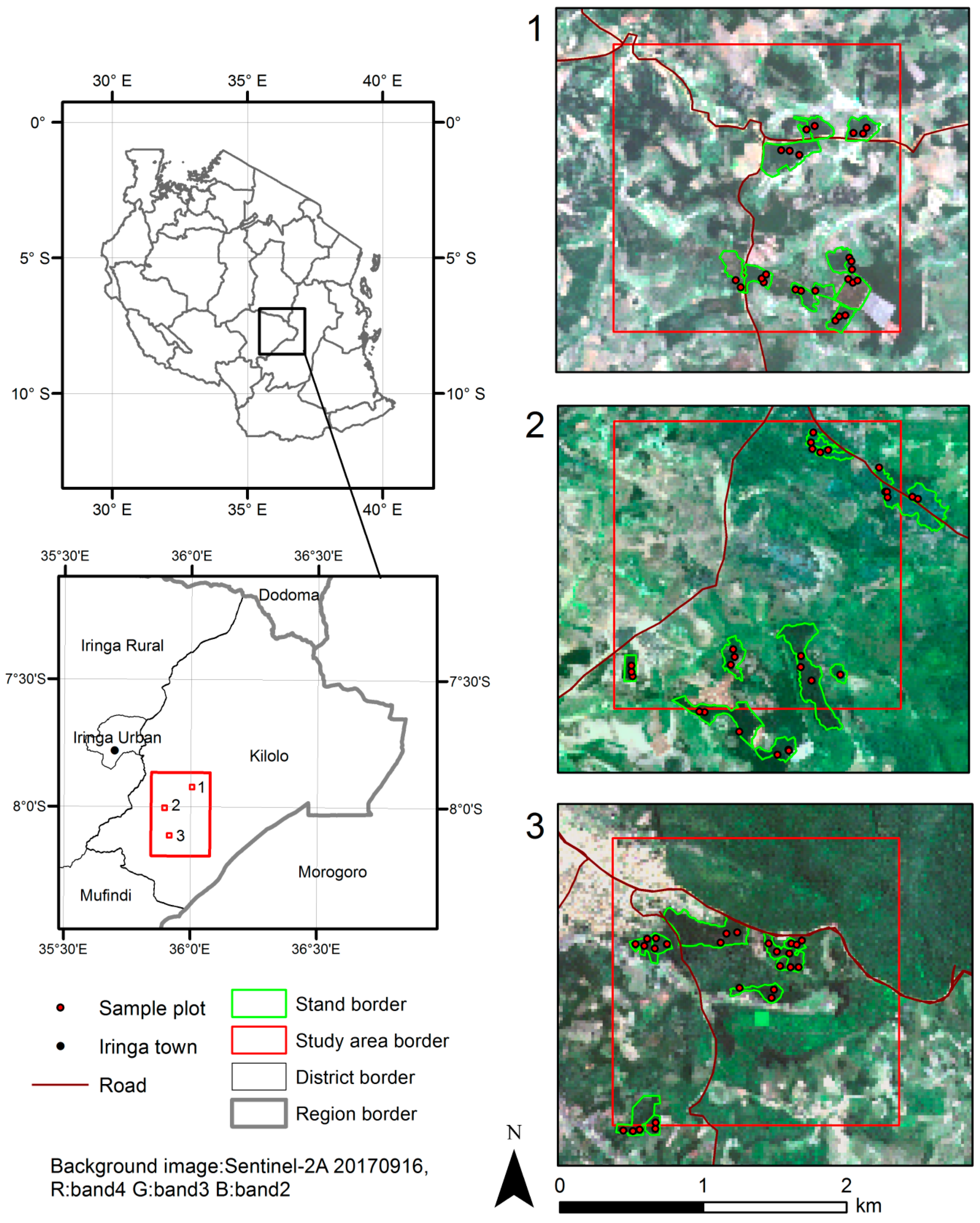
2.1. Study Area

Our study was conducted in the Kilolo district, one of five administrative units of the Iringa Region, in the Southern Highlands of Tanzania. Kilolo district makes up the eastern part of the Iringa region, bordering Dodoma region to the north and Morogoro region to the East and South (Figure 1). Much of the district is mountainous, with steep hills, ridges, valleys and escarpments. Its altitude ranges from 900 m to 2500 m above the sea level, and it is covered by alluvial soil. The precipitation pattern is unimodal starting in November and continuing until April with a yearly average of 1000 mm [32]. Due to the reliable and sufficient rains, the conditions are favourable for silviculture and the forest plantation area has been growing rapidly [28,29]. Tree planting is practiced by a multitude of stakeholders, including the central government, district councils, village governments, military forces, private forest companies, NGOs, schools, and families [33]. Most of the present and emerging forest plantations are small-scale, they are scattered in the landscape, and their GSV is largely unknown. For effective management plans of the forest sector’s entire value chain, GSV estimations are crucial in the area. As the forest plantation landscape is fragmented, field inventories are time-consuming. Thus, there is a need to test how well Earth observation-based estimations work within the area.

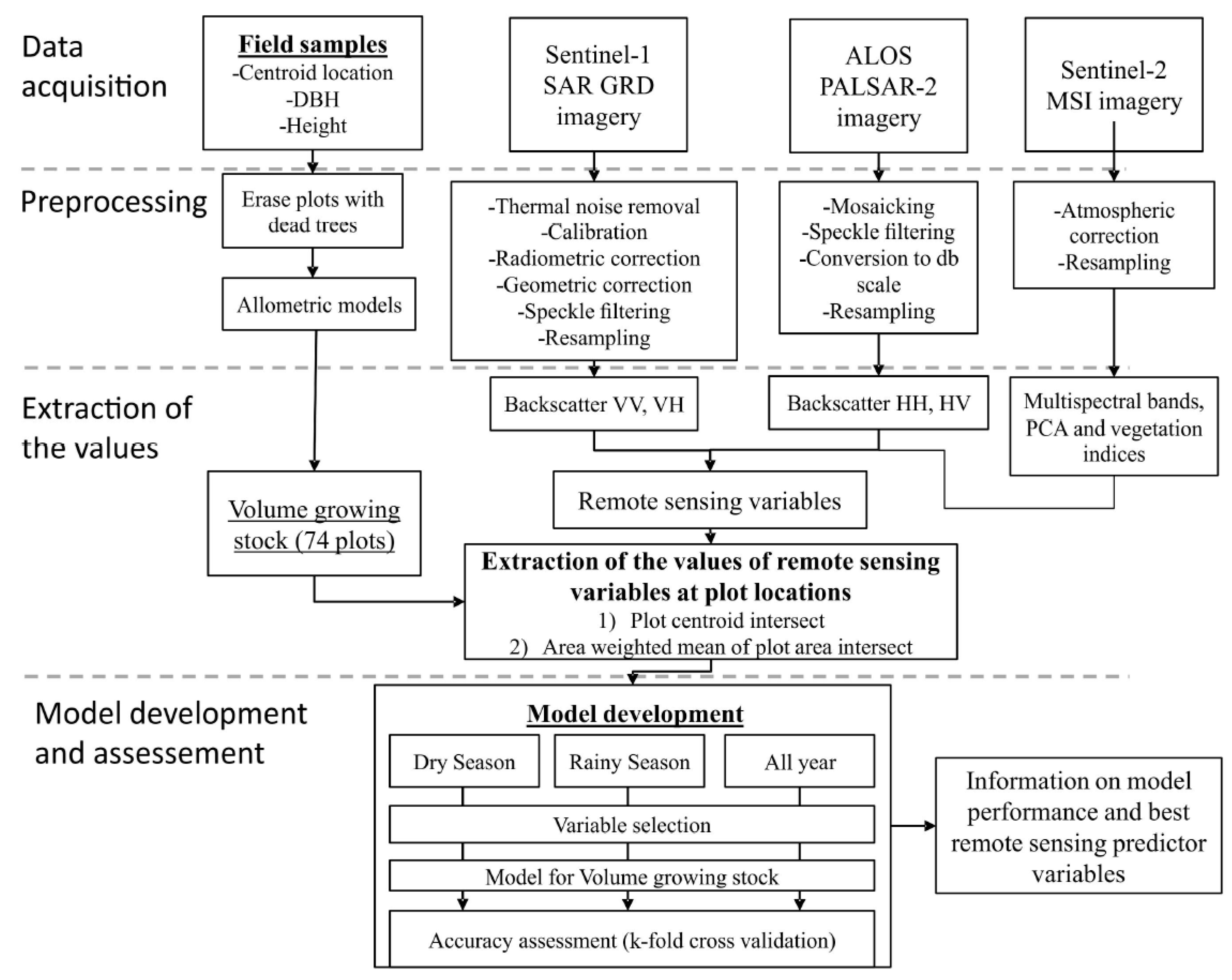
2.2. An Overview of the Study Design

We assessed the potential of multiple open access data sources in a remote-sensing assisted forest inventory. The approach can be divided into four phases: (1) Acquisition of field plot data and remote-sensing imagery, (2) preprocessing of the field measurements and the remote-sensing imagery, (3) extracting the values of remote-sensing variables at plot locations, and (4) developing predictive models of different variable set ups and assessing their accuracy via cross validation (Figure 2). The sections below describe the phases in more detail.

2.3. Sampling Design

Two-phase stratified sampling was used to design this study. In the first phase, we identified locations with large variation of plantation tree species. The forest stands were created based on the previous plantation mask produced by the Private Forestry Program (PFP) (Mankinen, Käyhkö, Koskinen and [29]. Then, the Kilolo study window was divided into regular 2 km × 2 km blocks, and 3 sample blocks were selected based on accessibility, variation, and the amount of stands in all classes (Figure 1).

In the second phase, 10 stands, representing each category (Pinus patula, Eucalyptus spp, and others) were randomly chosen from the three blocks. Stands smaller than 0.5 hectares, were omitted. Three sample plots were randomly placed within each stand. A 15 mthreshold from stand border was used to avoid creating a plot close to the stand border. Hand held GPS receivers were used to find the central coordinate position of the sample plots.

2.4. Field Data Collection and Processing

Seventy-seven (77) circular plots with 10 m radii, representing approximately ten sample candidates from each sample block, were established and measured across the entire area of interest in a field campaign conducted in March of 2018. The plot center location was marked and recorded with a handheld GPS. All the trees in the plots were measured for diameter at breast height (DBH) using a caliper or diameter tape, depending on the tree’s size, only trees with DBH ≥ 5 cm were considered for measurements. Species names were recorded for every tree measured for DBH. Every fifth tree in the plot was selected as a sample tree and measured for height using a Vertex hypsometer.

For trees without height measurements, tree height was predicted according to height-diameter (H-D) models constructed from the sample trees. The volume of individual trees within each plot was calculated using vegetation and species specific allometric models [34,35,36,37]. The volume for all the trees within the plot were summed to obtain total GSV for the respective plot and then scaled to per-hectare values according to their respective plot area. Three of the plots had entirely dead trees and therefore were eliminated from further analysis. The calculated GSVs (m³/ha) for the seventy-four (74) plots are henceforth denoted as field measured GSV. Since Pinus patula was the most dominant tree species, we further aggregated our plots into two major groups of Pinus patula and others. The summarized statistics of the plot-level values for the two groups are presented in

Table 1. Summary statistics for the growing stock volume.

Descriptive Statistics	Pinus spp.	Others	All
Minimum (m3/ha)	40.1	6.4	6.4
Mean (m3/ha)	163.2	186.7	172.7
Maximum (m3/ha)	308.4	660.2	660.2
Standard deviation (m3/ha)	51.2	167.2	113.1
Number of field plots	44	30	74

as part of the data descriptions. These data were then used to model GSV using Sentinel-1, Sentinel-2, and ALOS PALSAR-2 remote-sensing data.

2.5. Satellite Images

2.5.1. Sentinel-2

Sentinel-2 satellites carry a Multi-Spectral Instrument (MSI) to scan the earth with 13 spectral bands, a 290 km wide swath, and a five day revisit frequency at the equator [38]. We acquired Level-1C products via Google Earth Engine platform with a restricted study area. Our aim was to retrieve images representing the previous dry season and the present rainy season related to the field campaign’s timing (

Table 2. List of images acquired for the study, divided into dry season, rainy season, and all year acquisitions.

Time	Product	Observation Date	Cell Size (m)	Polarisa-tion/Ex-Tracted Bands	Relative Orbit
Dry Season	Sentinel-1A Level-1 GRD	5 June 2017, 17 June 2017, 29 June 2017, 11 July 2017, 23 July 2017, 4 August 2017, 16 August 2017, 28 August 2017, 9 September 2017, 21 September 2017, 3 October 2017, 15 October 2017, 27 October 2017, 8 November 2017, 20 November 2017	10	VV,VH	28
	Sentinel-2A Level-1C MSI	16 September 2017	10,20	B2-B8A, B11,B12	92
Rainy Season	Sentinel-1A Level-1 GRD	12 May 2017, 24 May 2017, 2 December 2017, 14 December 2017, 26 December 2017, 7 January 2018, 19 January 2018, 31 January 2018, 12 February 2018, 24 February 2018, 8 March 2018	10	VV,VH	28
	Sentinel-2B Level-1C MSI	18 February 2018	10,20	B2-B8A, B11,B12	92
All year	ALOS PALSAR mosaic	2017	25	HH,HV

). The images were corrected to the bottom-of-atmosphere (BOA) with a simple Dark Object Subtraction 1 (DOS1) algorithm using a semiautomatic classification plugin in QGIS [39].

All the visible bands (B02, B03, and B04), the Near-Infrared (NIR), and red edge bands (B08, B08a, B05, B06, and B07), and the Shortwave Infrared (SWIR) bands (B11 and B12) of the images were extracted for further analysis. For the spectral band values, we also calculated the principal components (PC) and the vegetation indices (

Table 3. Vegetation indices calculated from the Sentinel-2 images.

Index	Name	Formula	References
NDVI	Normalized Difference Vegetation Index	(B08-B04)/(B08+B04)	[43]
EVI	Enhanced Vegetation index	2.5*(B08 − B04)/(B08 + 6 × B04 − 7.5*B02 + 1)	[44]
RE-NDVI740	Red-Edge Normalized Difference Vegetation index 1	(B08 − B06)/(B08 + B06)	[45]
RE-NDVI783	Red-Edge Normalized Difference Vegetation index 2	(B08 − B07)/(B08 + B07)	[40]
RE-NDVI705	Red-Edge Normalized Difference Vegetation index 3	(B08 − B05)/(B08 + B05)	[41]
ND-RE1	Normalized Difference Red-Edge 1	(B06 − B05)/(B06 + B05)	[40]
ND-RE2	Normalized Difference Red-Edge 2	(B07 − B05)/(B07 + B05)	[40]
CHL-RE	Chlorophyll Red-Edge	(B07/B05) − 1	[40]
PC	Principal component	PCA
			[46]

Note: B02, B04, B05, B06, B07 and B08 refer to Sentinel-2 MSI spectral bands with central wavelengths of 490 nm, 665 nm, 705 nm, 740 nm, 783 nm, and 842 nm, respectively.

). The calculated vegetation indices were chosen to evaluate the potential of the bands operating in the NIR and red edge spectrum because bands operating at these wavelengths have been found to effectively predict forest characteristics in a number of recent studies [13,40,41,42]. The first three first PCs were extracted for further analysis as they explained 99% of the total variance. The spectral bands, the first three PCs and vegetation indices were derived and calculated for Sentinel-2 images, representing dry and rainy seasons (Table 2).

2.5.2. Sentinel-1

Sentinel-1 satellites carry a C-band SAR instrument that collect data in four modes. The standard Interferometric Wide Swath (IW) mode operates on land observing in single and dual polarization [9]. We used the available Level-1 IW Ground Range Detected (GRD) dual-polarised VH (vertical transmit-horizontal receive) and, VV (vertical transmit-vertical receive) imagery with spatial resolution of 10 m, acquired from the Copernicus Open Access Hub of ESA (https://scihub.copernicus.eu/dhus/). The retrieved images were representing the closest date compared to the sensing date of the optical images and the field campaign. To evaluate the predictive value of C-band SAR imagery in the temporal dimension, we acquired images to create datasets representing the dry season (15 images between June 2017 and November 2017), the rainy season (11 images from May 2017 and between December 2017 and March 2018) (Table 2) and all year (dry season and rainy season images combined). The temporal statistics of mean, maximum (max), minimum (min), standard deviation (std), and coefficient of variation (cv) of these Sentinel-1 composites were calculated and named as dry season timescan, rainy season timescan, and Annual timescan [47]. Sentinel-1 SAR images were pre-processed using Sentinel Application Platform tool (SNAP). The pre-processing steps included (1) thermal noise removal, (2) image calibration, (3) radiometric and geometric correction to acquire orthorectified backscatter images with reduced effect of topography to radiometric variability, and (4) Lee sigma speckle filtering, in order to derive gamma-naught backscatter values (dB).

2.5.3. Global ALOS PALSAR-2/PALSAR Mosaic

The Japanese Aerospace Exploration Agency (JAXA) provides yearly global mosaics of Advanced Land Observing Satellite (ALOS) dual-polarised HH (horizontal transmit-horizontal receive), HV (horizontal transmit-vertical receive) L-Band SAR backscatter data on a yearly basis [10]. The data tiles from 2017, covering the study area, were merged, filtered, and converted to decibel scale [10,48] using SNAP tool. In addition, we calculated the subtract-channel (HH-HV) to enhance the visualisation and information extraction.

2.6. Extraction of the Satellite Image Values

To ensure spatial overlap between the measured GSV at the 10 m plot and the information acquired from the remotely sensed data, we co-registered and resampled the remote-sensing dataset to the spatial resolution of a 20 m using a bilinear interpolation algorithm that uses the values of the four closest cells to calculate a weighted average for the new cell. We then tested two methods of variable extraction from the remotely sensed data: (1) Extracting the value of the predictor variable from the pixel containing the plot centroid, (i.e., centroid approach), and (2) extracting the value of the predictor variable as the weighted mean value of the pixels intersecting with the plot area (i.e., weighted mean approach). All the variables extracted from remotely sensed data using the two methods are presented and defined in the Supplementary Material.

2.7. Statistical Modelling

2.7.1. Model Development

An Ordinary Least Square regression (OLS), was used to develop the predictive models which relates the field measured GSV and the remote-sensing predictor variables. Model development was done using a set of predictor variables for Sentinel-1, Sentinel-2 and ALOS PALSAR mosaic which were computed using centroid (denoted MC) and area weighted mean (denoted MW) approaches. To test the effect of seasonality, the predictor variables were categorized into: (1) All year (A), (2) dry season (DS), and (3) rain season (RS).

Table 4. Data and predictor variable categories used for modelling.

Predictor Category	Description	Data	Number of Variables
A1	Annual Sentinel-1	Sentinel-1 20170921 (bands) & Sentinel-1 20180212 (bands) & Sentinel-1 Annual timescan (bands)	9
A2	Annual Sentinel-2	Sentinel-2 20170916 (bands, PCs, indices) & Sentinel-2 20180218 (bands, PCs, indices)	42
A3	Annual ALOS	ALOS PALSAR mosaic 2017 (bands)	2
A4	Annual Sentinel-1 & 2	Sentinel-2 20170916 (bands, PCs, indices) & Sentinel-2 20180218 (bands, PCs, indices) & Sentinel-1 20170921 (bands) & Sentinel-1 20180212 (bands) & Sentinel-1 Annual timescan (bands)	51
A5	Annual Sentinel-2 & ALOS	Sentinel-2 20170916 (bands, PCs, indices) & Sentinel-2 20180218 (bands, PCs, indices) & ALOS PALSAR mosaic 2017 (bands)	44
A6	Annual Sentinel-1 & ALOS	Sentinel-1 20170921 (bands) & Sentinel-1 20180212 (bands) & Sentinel-1 Annual timescan (bands) & ALOS PALSAR mosaic 2017 (bands)	11
A7	Annual Sentinel-1 & 2 & ALOS	Sentinel-1 20170921 (bands) & Sentinel-1 20180212 (bands) & Sentinel-1 Annual timescan (bands) & Sentinel-2 20170916 (bands, PCs, indices) & Sentinel-2 20180218 (bands, PCs, indices) & ALOS PALSAR mosaic 2017 (bands)	53
DS1	Dry season Sentinel-1	Sentinel-1 20170921 (bands) & Sentinel-1 Dry season timescan (bands)	7
DS2	Dry season Sentinel-2	Sentinel-2 20170916 (bands, PCs, indices)	21
DS3	Dry season Sentinel-1 & 2	Sentinel-1 20170921 (bands) & Sentinel-1 Dry season timescan (bands) & Sentinel-2 20170916 (bands, PCs, indices)	28
RS1	Rainy season Sentinel-1	Sentinel-1 20180212 (bands) & Sentinel-1 Rainy season timescan (bands)	7
RS2	Rainy season Sentinel-2	Sentinel-2 20180218 (bands, PCs, indices)	21
RS3	Rainy season Sentinel-1 & 2	Sentinel-1 20180212 (bands) & Sentinel-1 Rainy season timescan (bands) & Sentinel-2 20180218 (bands, PCs, indices)	28

further summarizes the data used and the predictors categories.

To ensure that we develop robust models for different datasets and predictor variables, we first performed a variable selection as a critical step in modelling the combination of field and remote-sensing data [see 16]). Candidate predictor variables for each category presented in Table 4, were selected using regsubset function implemented in the “leaps” package [49] of the R statistical software [50]. The regsubset is an automated approach where all possible variable combinations are considered and ranked based on different scoring criteria (adjusted R², Mallow’s Cp statistics, BIC, etc.) [51]. In this study, we used Mallow’s Cp statistics [52]. A Combination of predictors that minimized the Mallow Cp over all possible subsets, was considered as the best subset for model development. The best subsets were then used to fit the models and the variables were further assessed based on their significance (i.e., p < 0.05) and variance inflation factor (VIF). Predictor variables with a VIF value greater than ten were considered to be a source of multicollinearity [53] and hence were trimmed out from the model. The procedure was done repeatedly for all the categories of the predictor variables presented in Table 4. However, we had exceptional cases with categories combining Sentinel 1 and Sentinel-2 derived variables, where all the variables from Sentinel-1 were not selected in the best subset. As our interest was to look at the potential of combining Sentinel-1 and Sentinel-2, we combined the best subset from Sentinel 1 with those from Sentinel-2. The combined best subsets were then further assessed based on the significance of the predictor variables, as well as VIF values. As part of the model fitting procedure we also calculated a pseudo-R² from the residual sum of squares (RSS) and the total sum of squares (TSS). That is,

$$\mathrm{pseudo}-{\mathrm{R}}^2=1-\left(\frac{\mathrm{RSS}}{\mathrm{TSS}}\right)$$

Residual diagnostic plots were examined for each of the fitted model and the Akaike Information Criteria (AIC) was computed for each of the fitted model. The importance of each variable in the model was determined using the “relaimpo” package in R [54]. This was essentially aimed to understand how individual predictor variables contribute to the model fit. Finally, the models were subjected into cross validation, as described in the section below.

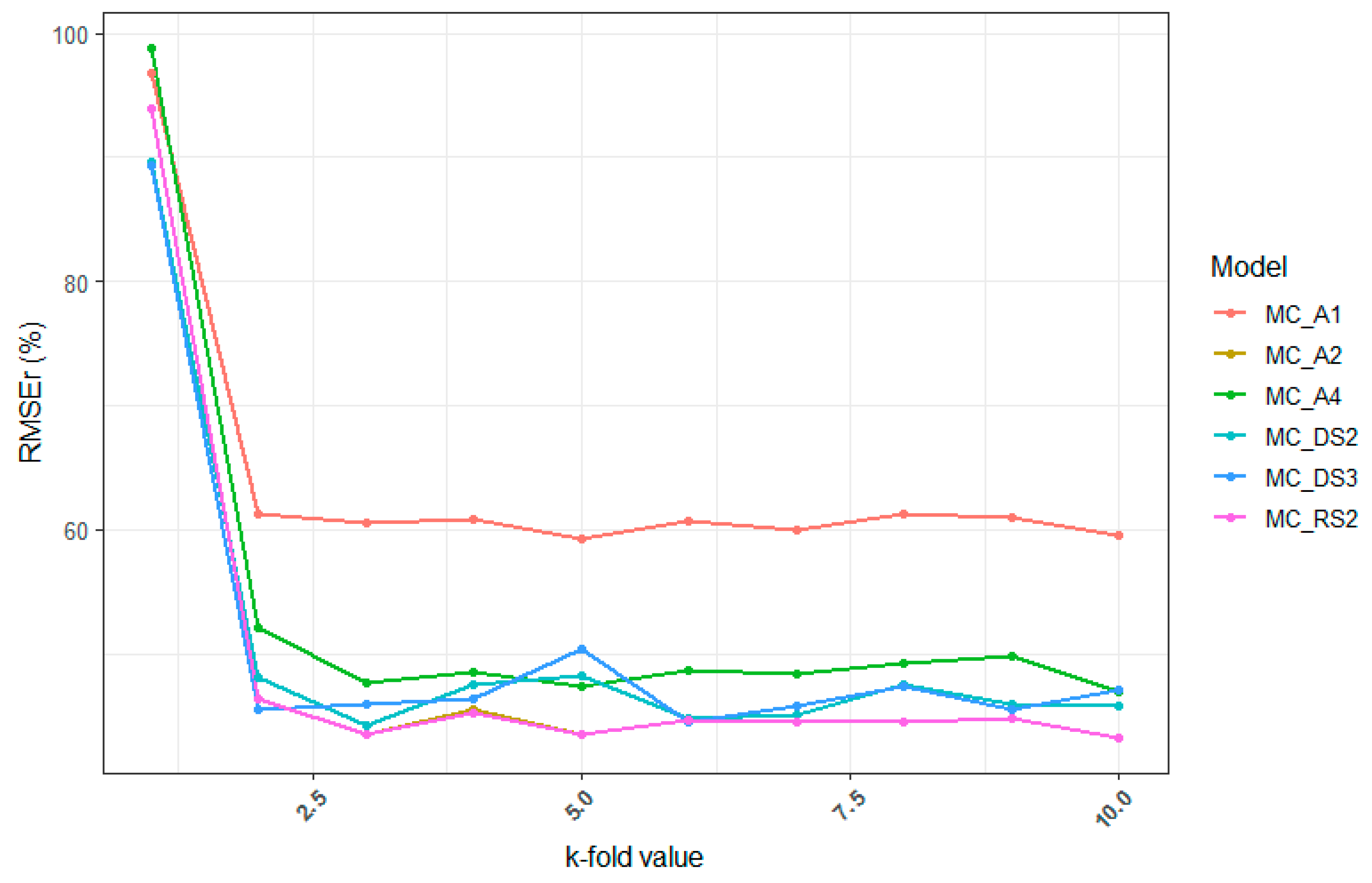
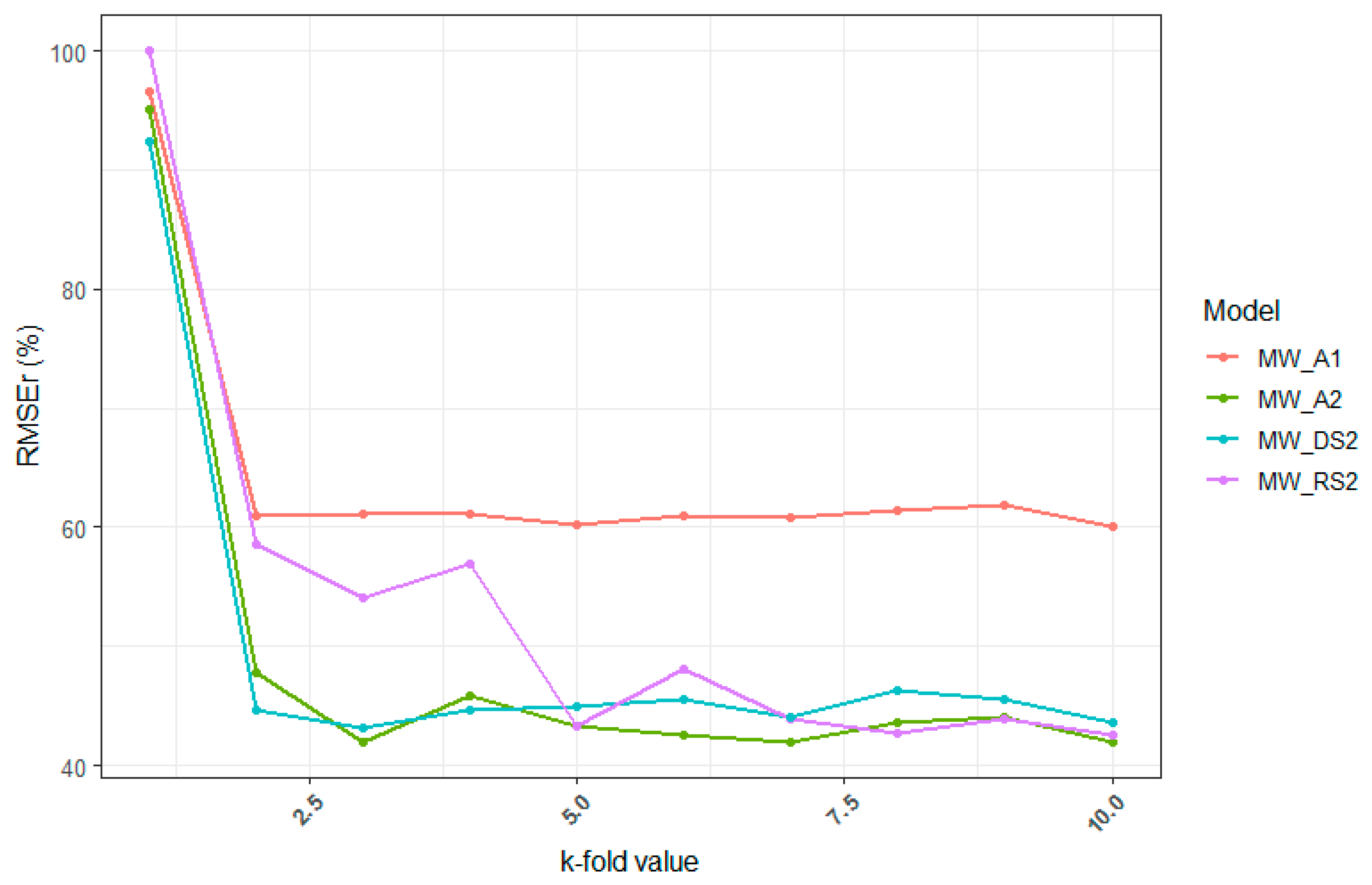
2.7.2. Model Validation

To enable comparison among the models developed from different groups of predictor variables (Table 4), and to understand the models performance on other datasets, the models were cross-validated. Ideally, in order to perform model validation, the independent datasets for model validation should be drawn from the population in which the model will be applied. However, due to the limitations in field data availability in our study area, we implemented a k-fold cross validation. We used a k-value of 10 because it had been widely used and empirically shown to yield test error rate estimates that do to suffer from excessively high bias from very high variance [55,56]. The 10-fold cross-validation involves splitting the dataset into 10-subsets. In each fold, one subset is held out to check the model performance (i.e., the validation set), while the model is trained on all other subsets (i.e., 9 subsets). The process is repeatedly done until all the subsets have been used once as the validation dataset.

The predicted values from all the folds were finally compiled into a table and used to estimate measures of reliability. We used the absolute and the relative root mean square error as the most common statistic to characterize the error of remote-sensing based forest AGB and GSV models [57]. The root mean square error (RMSE) and the relative root mean square error (RMSEr) were calculated as,

$$\mathrm{RMSE}=\sqrt{{{\displaystyle \sum }}_{\mathrm{I}=1}^{\mathrm{n}}\frac{{\left({\mathrm{y}}_{\mathrm{i}}-{\widehat{\mathrm{y}}}_{\mathrm{i}}\right)}^2}{\mathrm{n}}}$$

and

$${\mathrm{RMSE}}_{\mathrm{r}}=\frac{\mathrm{RMSE}}{\overline{\mathrm{y}}}\times 100\%$$

where $y_i$ and $\widehat{y}$ denote the field measured GSV and the predicted volume for plot i, respectively, and $\overline{y}$ denotes the mean field measured GSV for all plots. The RMSE and the RMSE_r from the cross validation were compared among the different model categories. The RMSEr values were also displayed for different values of k-folds ranging from 1 to 10, to show the stability of the models.

Finally, to reflect the performance of models fitted with Sentinel data under different tree species, we partitioned the prediction values obtained from the cross validation into two groups (i.e., Pinus patula and others). The predicted values were then used to compute the RMSE and the RMSEr as illustrated above, and model performances were compared.

3. Results

3.1. Prediction Accuracy of GSV for Different Sets of Predictor Categories and Models

Variables between two and five were selected from different categories of predictor variables (

Table 5. Fitted models, selected variables from the centroid approach (MC), Pseudo-R², AIC, RMSE, and RMSEr.

Model a	Selected Variables b	Pseudo-R2	AIC	RMSE	RMSEr
MC_A1	M6_DS, S1_18_M2	0.18	902	103	59.48
MC_A2	M4__18f18, M12__18f18, ndvi2_18	0.59	853	75	43.17
MC_A4	M4__18f18, M11__18f18, M6_Annua, M1_DS	0.52	866	81	46.98
MC_DS2	M5_17s16, M11_17s16, NDRE1_17	0.57	857	79	45.80
MC_DS3	M5_17s16, M11_17s16, NDRE1_17, M9_DS	0.59	855	81	47.07
MC_RS2	M4__18f18, M12__18f18, ndvi2_18	0.59	853	75	43.17

Notes: ^a MC_A1 = Model fitted with S1_20170921 & S1_20180212 & Annual times can data, MC_A2 = Model fitted with S2_20170916 & S2_20180218 data, MC_A4 = Model fitted with S2_20170916 & S2_20180218 & S1_20170921 & S1_20180212 & Annual time scan data, MC_DS2 = Model fitted with S2_20170916 (i.e., Dry Season) data, MC_DS3 = Model fitted with S1_20170921 & Dry season time scan & S2_20170916 data, MC_RS2 = S2_20180212 (i.e., Rain season) data. ^b M6_DS = Dry season Sentinel-1: VH_min, S1_18_M2 = Sentinel 1_20180212_VV, M4__18f18 = Sentinel2_20180218_B08a, M12__18f18 = Sentinel2_20180218_B12, ndvi2_18 = Sentinel-2_20180218:RE-NDVI₇₈₃, M6_Annua = Annual Sentinel-1: VH_min, M4__18f18 = Sentinel-2_20180218:B04, M5__18f18 = Sentinel-2_20180218: B05, M11__18f18 = Sentinel2_20180218_B11, M6_Annua = Annual_time scan Sentinel 1 band6: VH_min, M1_DS = Dry season time scan Sentinel 1 band1: VV_mean, M5_17s16 = Sentinel2_20170916_ B05, M11_17s16 = Sentinel2_20170916_ B11, NDRE1_17 = Sentinel-2_20170916:ND_RE1, M9_DS = Dry season Sentinel-1: VV_cv.

and

Table 6. Fitted models, selected variables from weighted mean approach (MW), Pseudo-R², AIC, RMSE, and RMSEr.

Model a	Selected Variables b	Pseudo-R2	AIC	RMSE	RMSEr
MW_A1	M6_DS, S1_18_M2	0.17	903	103.8	60.10
MW_A2	M5_17s16, M11_17s16, M4__18f18 M11__18f18, ndvi7_18	0.63	849	72.6	42.03
MW_RS2	M2__18f18, M4__18f18, M12__18f18, ndvi1_18	0.61	850	73.4	42.52
MW_DS2	M5_17s16, M11_17s16, evi17, NDRE1_17	0.58	855	75.4	43.65

Notes: ^a MW_A1 = Model fitted S1_20170921 & S1_20180212 & Annual times can data, MW_A2 = Model fitted with S2_20170916 & S2_20180218 data, MW_RS2 = Model fitted with S2_20180212 (i.e., Rain season) data, MW_DS2 = Model fitted with S1_20170921 and Dry season time scan and S2_20170916 data. M6_DS = Dry season Sentinel-1: VH_min, S1_18_M2 = Sentinel 1_20180212_VV, M5_17s16 = Sentinel-2_20170916:B05, M11_17s16 = Sentinel-2_20170916:B11, M4__18f18 = Sentinel-2_20180218:B04, M11__18f18 = Sentinel-2_20180218:B11, ndvi7_18 = Sentinel-2_20180218:RE-NDVI₇₀₅, M2__18f18 = Sentinel-2_20180218:B02, M4__18f18 = Sentinel-2_20180218:B04, M11__18f18 = Sentinel-2_20180218:B11, M12__18f18 = Sentinel-2_20180218:B12, ndvi1_18 = Sentinel-2_20180218:RE-NDVI₇₄₀, evi17 = Sentinel-2_20170916:EVI, NDRE1_17 = Sentinel-2_20170916:ND_RE1.

). All predictors were derived from categories with Sentinel-1 and Sentinel-2 bands, derived indices, and their combination. Predictor variables for the ALOS PALSAR mosaic were not statistically significant in any model and are not presented in the result section.

The fits of the selected models, judged by Pseudo-R² and AIC values, and the selected variables vary depending on the predictor category and the variable extraction method (Table 5 and Table 6). The Pseudo-R² ranges from 0.18 to 0.59 for the models fitted with the MC approach and from 0.17 to 0.63 for the MW approach. Combining Sentinel-1 and Sentinel-2 when using MC based predictor variables improved the model fits compared with Sentinel-1 alone. When developing the model by combining Sentinel-1 and Sentinel-2 using the MW approach, all the possible predictor variables of Sentinel-1 were not significant in the model. It was, therefore, nearly impossible to develop a model combining Sentinel-1 and 2 when using the MW approach. The selected variables, Pseudo-R², AIC, RMSE, and RMSEr of the fitted models are presented in Table 5 and Table 6. The variable importance of the different predictors in each model are also presented in Figure 3 and Figure 4, where the variables from bands (B11 and B12) largely contributed to R² and were frequently selected.

The results from the cross validation indicated that, the RMSEr values for models fitted with combined variables extracted from the MC approach for Sentinel-1 and Sentinel-2, were relatively lower than the model fitted with separate variables of Sentinel-1. This indicates a potential gain in accuracy when combining Sentinel-1 and Sentinel-2 when using the variable extracted from the MC approach. However, the models with Sentinel-2 variables extracted using MC and MW variables, turned out to be the best with the lowest RMSEr values. The sensitivity of the RMSEr values of different models to the k-fold values are presented in Figure 5 and Figure 6. The k-values of 3, 5, and 10 turned out to have the lowest RMSEr values. However, for fair comparison among models the results presented in Table 5 and Table 6 are based on 10-folds only. The performance of the models for each variable extraction method are further explained with the scatterplots showing the relationships between the field measured GSV and the predicted GSV (Figure 7 and Figure 8).

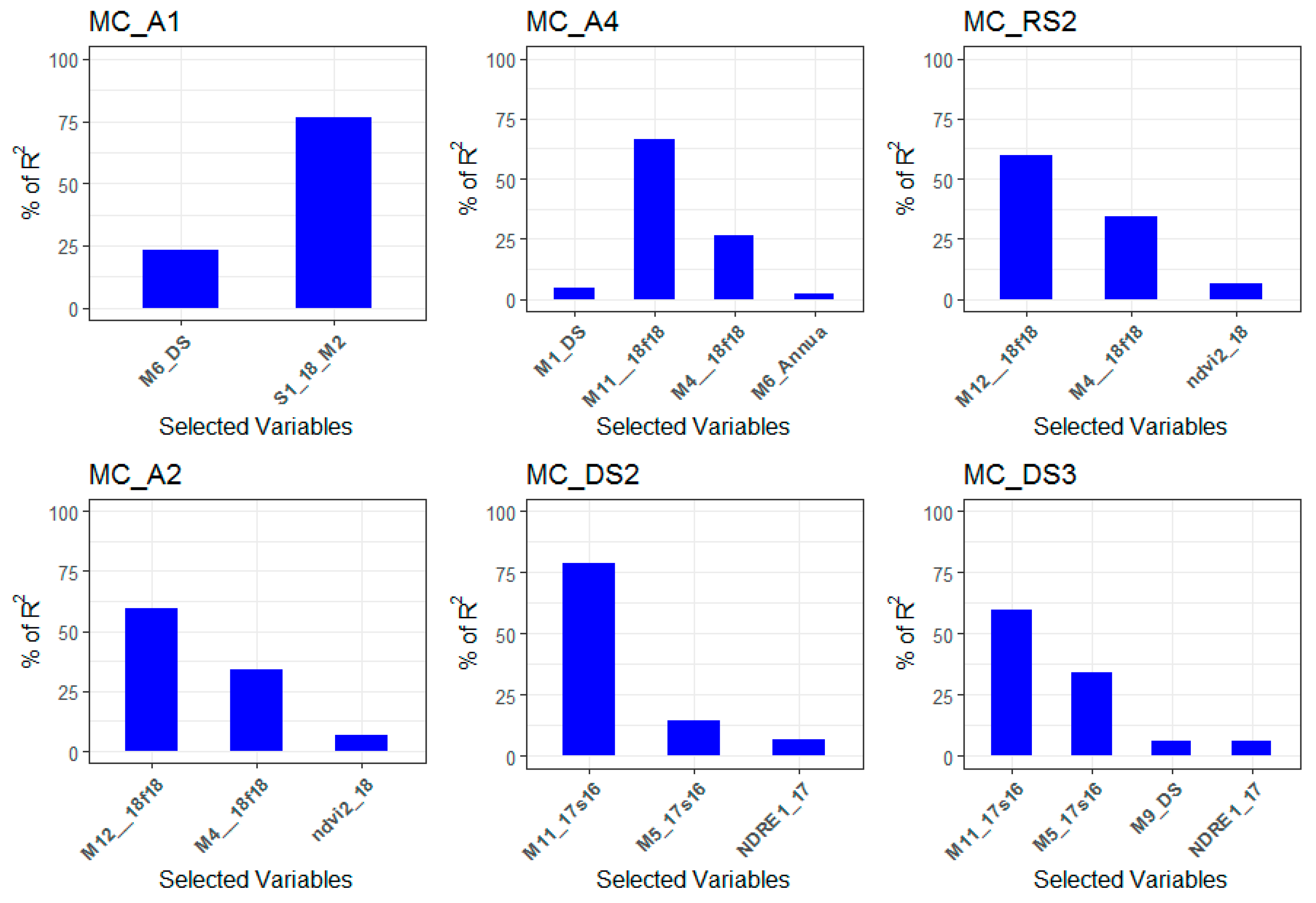
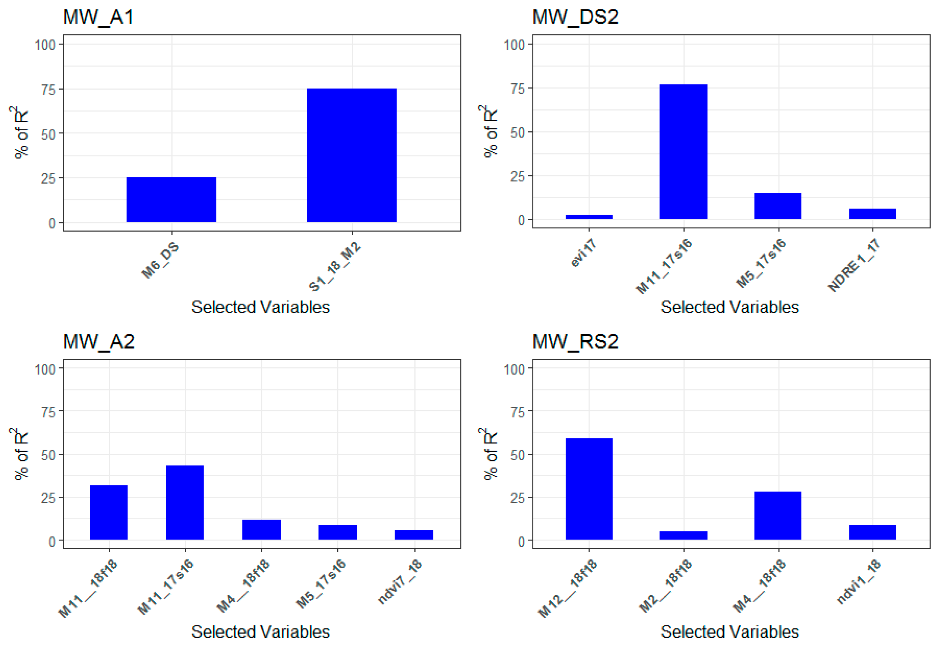
3.2. The Effect of Season and Specific Predictor Variables on GSV Prediction Accuracy

Pseudo-R², RMSE, and RMSEr for the seasonal based models fitted with variables extracted using the MC and the MW approaches are presented in Table 5 and Table 6. The results showed that using Sentinel-1 with season-based predictor variables did not turn up to have good linear relationships, especially when using the predictors extracted with the MC approach. All the selected variables were not statistically significant (i.e., p > 0.005) in the models. A combination of Sentinel-1 and Sentinel-2 DS predictors had reasonable accuracy compared with Sentinel-1 DS only. Poor results for Sentinel-1 DS were also observed when using variables extracted with the MW approach. Sentinel-2 models, fitted with RS predictor variables, had a lower RMSEr compared with the models fitted using the DS for both of the approaches of the variable extraction. Furthermore, there was no difference in terms of model fits and accuracy, for the models MC_A2 and MC_RS2 (Table 5). However, a notable marginal difference was observed when using the MW approach where the model MW_A2 had relatively smaller RMSEr than the model MW_RS2 (Table 6). Thus the overall best model (MW_A2) was based on all year predictor variables.

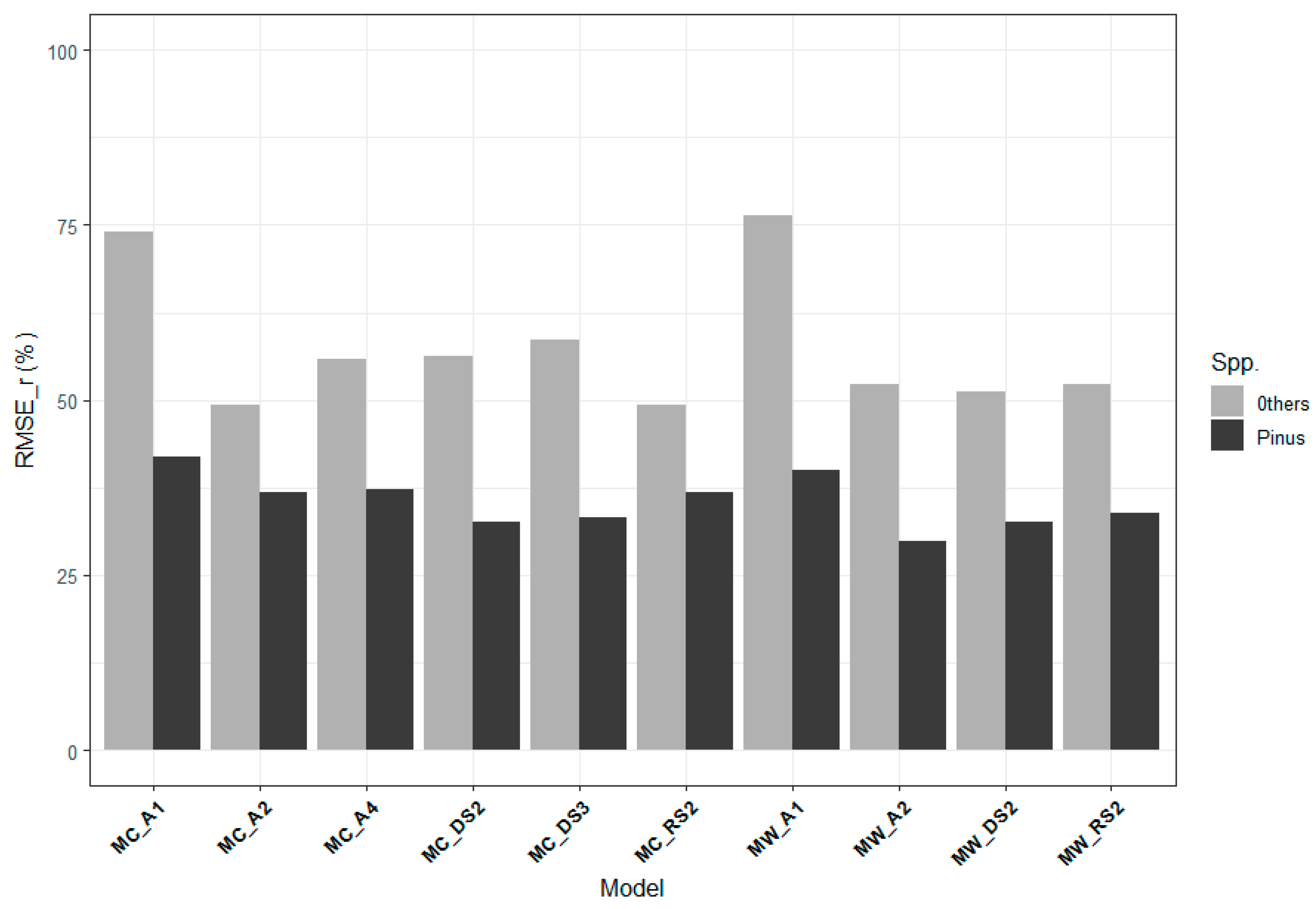
3.3. Effects of Post Stratification on Prediction Accuracy of GSV

Our results on the effect of post-stratification on prediction accuracy indicated that there were variations in the prediction accuracy between the two groups of tree species irrespective of the method of variable extraction. The RMSE_r values for all models in the Pinus spp group were relatively lower, as compared with the other tree species group (Figure 9).

4. Discussion

The main objective of the study was to determine the potential of the Sentinel imagery in predicting GSV, the most common forest stand variable needed for sustainable forest management and reporting on national and international scales. Predictive models built on open-source data and tools are especially vital in Global South countries like Tanzania, where the forestry sector is growing rapidly, and the availability of intensive field inventory is limited. Thus, investigating the potential of open-source remotely sensed data in this area, including their combination, provides new information towards developing standard methods for generating reliable information to support forest management planning at a reasonable and affordable cost. Such methods are also important for the establishment of forest carbon Monitoring, Reporting, and Verification system needed for the implementation of the REDD+ programme of the United Nations Framework Convention on Climate Change.

Overall, our study has shown that, Sentinel-derived predictors have better performance in predicting growing stock volume in the heterogeneous small-scale plantation environment of the Southern Highlands compared with global ALOS PALSAR mosaic derived predictors. We used a yearly global mosaic of ALOS PALSAR-2/PALSAR, which is freely distributed and has coarser spatial and temporal resolutions compared with the regular ALOS imagery [17]. Although the global ALOS PALSAR mosaic data has previously shown to correspond with AGB at a wide geographical scale [58], the reason for the poor performance of SAR-L in our study area when modelling GSV may be related to the coarse spatial and temporal resolution that results in weak applicability on detailed plot-level.

For Sentinel imagery, the models based on optical imagery outperformed the models based on SAR-C imagery. Although, integration was found to increase the performance in one model (MC_A4), we may conclude that variables derived from Sentinel-1 performed weakly in GSV modeling at our study site. Sentinel-1′s prediction performance on forests has been shown to vary due to the SAR-C band sensitivity to the forest dielectric constant and the environment’s moisture conditions. Thus time-series applications are recommended [24,59]. Notably, most of the significant variables in models based on Sentinel-1 in our study were derived from a dry season multi-temporal composite. However, a more detailed time series analysis would have been required to reveal the optimal timing of Sentinel-1′s response to GSV. Nevertheless, the predictor’s contributions to R^2′ values were so small that even optimal timing would unlikely result in applicable predicting capacity (Figure 3 and Figure 4). Another reason for poor performance may be the saturation of SAR-C backscatter at relatively low biomass density levels. However, since SAR-L band predictor were not selected to the models due to their low prediction power and SAR-L backscatter saturates at much higher AGB density levels compared to SAR-C [24], it is likely that the poor prediction power of SAR-C backscatter on GSV is also affected by complex backscatter signal from the studied forests due to speckle noise.

Models based on Sentinel-2 had the best predicting performance considering all the categories: dry season, rainy season, and all year. This is further explained by the variable importance where the Sentinel-2 variables had most significant contributions to R² (Figure 3 and Figure 4). While there was only a small difference in the overall performance of these models, there were notable differences on the selected variables within the models of different categories. For all year and rainy season category models, the most important bands were 11 and 12 operating on the SWIR wavelength and bands 5 and 4 operating on red edge and red wavelengths, respectively. The potential of these bands in quantifying forest biophysical parameters has been reported by other studies concentrating on forest attribute modeling based on Sentinel-2 data [13,15,60]. SWIR band values are sensitive to moisture and shade conditions, which are more inherent to forest stand structures during the rainy season, as compared to the dry season. However, the high prediction potential of SWIR bands were missing in our best model of dry season category, where band 8A, operating on narrow infrared wavelength was the most important variable. In our case, the bands and indices of the red-edge wavelength (band 5 and NDRE-1) were important predictors in dry season models. The bands and indices of the red and NIR wavelength (band 4 and NDVI) were important predictors in rainy season models This result indicates that environmental conditions have a significant influence on the reflectance characteristics of plantation forests. The robustness of Sentinel-2 bands for forest attribute modeling need to be considered for the particular case.

The effect of the value extraction method on the selected variable and on the model performance proved to be significant. The performance of all the models based on Sentinel-2 improved when fitted with the variables extracted from the MW approach compared with the MC approach (Table 5 and Table 6). Geo-location errors up to 10 m are common when using GPS receivers to measure a plot centroid location under forest canopy [61]. In our study, the circular plot with a 10 m radius may result into mismatch between field and remote-sensing data, and hence increasing the errors in the models [62,63]. This is mainly because the plot centroid may locate in a pixel that shares only partly or none of the plot area. Thus, the MW extraction method is a more credible representation of the plot’s reflectance. Considering that the variables selected in the models MC_RS2 and MW_RS2 differ remarkably and are defined only based on the extraction method, so the value extraction approach is a key step in developing remote-sensing based predictions.

Comparing the results with other studies builds an understanding of the technical efficiency, but it should be done with caution due to the wide range of variations in the forest landscapes, forest structures, sample sizes and plot sizes used in different studies. The best combined model of Sentinel-1 and Sentinel-2 explained 52% of the variability in the data with RMSEr 46.98%. The best model from Sentinel-2 alone explained 63% of the variability in the data with RMSEr of 42.03 %. These values are comparable to other recent studies that predict GSV using Sentinel imagery [13,15,64] and RapidEye imagery in similar forested landscapes [65]. Post-stratification of the data into species showed that the best models have lower RMSEr values for Pinus patula compared with other tree species. This might be explained by the high variability of GSV in the “other” group because it contained plots from regenerating black wattle (Acacia mearnsii) to the presence of large eucalyptus tree species.

In our study, the Sentinel-2 derived GSV predictors outperformed the predictors derived from the SAR imagery. Similar results have been recently reported considering AGB estimation in tropical natural forest [66]. Sentinel-2 imagery thus has high potential to support large-scale, country wide forest assessments, especially in the Global South where expensive inventories and a lack of access to commercial satellite imagery has prohibited the development of sustainable forest management and spatially explicit estimations of forest GSV and AGB. Such potential is increasingly important, especially in tropics where forest plantations are rapidly growing in order to supply the increasing global demand for wood products and to support REDD+ processes as key strategies to mitigate climate change [67]. As the Sentinel-2 mission is operational, and providing high quality open-access data with a maximum of five days revisit time globally, it will definitely be the key source of information to support and assess such initiatives. However, the problems caused by frequent cloud cover, especially in the tropics, is a challenge in optical imagery based assessments. Future research is still needed to fully cover the potential of Sentinel-1 and Sentinel-2 missions and should examine the key parameters affecting the prediction accuracy, e.g., the effect of the field plot size and value extraction methodology. Furthermore, examining the performance of traditional statistical methods like linear regression, gives control and understanding on the predictive variables, important in evaluating the potential of the satellite imagery in GSV modelling. However, to fully cover the potential of the Sentinel imagery in forest attribute predictions, future studies should focus on studying the effect of statistical modelling methods on the prediction accuracy (i.e., parametric vs. non-parametric).

5. Conclusions

This study has generated empirical evidence on the use of Sentinel data in remotely sensing assisted forest inventory in the small-scale planation forests of Southern Highlands of Tanzania. The results show that: Sentinel-2 and combination of Sentinel-1 and 2, had better performance in predicting GSV, as compared to Sentinel-1 alone and ALOS PALSAR2. Models fitted with variables extracted from the WC approach, had relatively lower RMSEr % values compared with MC approaches. Season seemed to have effect on prediction accuracy of GSV when using Sentinel-2 where Sentinel-2 RS based models had slightly smaller RMSEr % values, as compared with DS based models. However, generally dense time series (i.e., annual) data resulted in the models with relatively lower RMSEr % values compared with seasonal based models. Stratifications based on tree species resulted into lower RMSEr % values for Pinus patula tree species as compared to other tree species. Thus in the future it might worthier to stratify the area based on the tree species using existing data, in order to account for the variability attributed by the differences in tree species. Further studies on the effect of field plot size and statistical methods on prediction accuracy are also recommended to further explore the potential of these data in supporting the estimation of forest attributes.

References

1. Mauya, E.W.; Ene, L.T.; Bollandsås, O.M.; Gobakken, T.; Næsset, E.; Malimbwi, R.E.; Zahabu, E. Modelling aboveground forest biomass using airborne laser scanner data in the miombo woodlands of Tanzania. Carbon Balance Manag. 2015, 10, 28. [Google Scholar] [CrossRef] [PubMed]
2. Mauya, E.W.; Mugasha, W.A.; Zahabu, E.; Bollandsås, O.M.; Eid, T. Models for estimation of tree volume in the miombo woodlands of tanzania. South. For. J. For. Sci. 2014, 76, 209–219. [Google Scholar] [CrossRef]
3. Næsset, E.; Ørka, H.O.; Solberg, S.; Bollandsås, O.M.; Hansen, E.H.; Mauya, E.; Zahabu, E.; Malimbwi, R.; Chamuya, N.; Olsson, H. Mapping and estimating forest area and aboveground biomass in miombo woodlands in tanzania using data from airborne laser scanning, tandem-x, rapideye, and global forest maps: A comparison of estimated precision. Remote Sens. Environ. 2016, 175, 282–300. [Google Scholar] [CrossRef]
4. Sinha, S.; Jeganathan, C.; Sharma, L.; Nathawat, M. A review of radar remote sensing for biomass estimation. Int. J. Environ. Sci. Technol. 2015, 12, 1779–1792. [Google Scholar] [CrossRef]
5. Zhao, P.; Lu, D.; Wang, G.; Liu, L.; Li, D.; Zhu, J.; Yu, S. Forest aboveground biomass estimation in zhejiang province using the integration of landsat tm and alos palsar data. Int. J. Appl. Earth Obs. Geoinf. 2016, 53, 1–15. [Google Scholar] [CrossRef]
6. Mauya, E. Methods for Estimating Volume, Biomass and Tree Species Diversity Using Field Inventory and Airborne Laser Scanning in the Tropical Forests of Tanzania. Ph.D. Thesis, Norwegian University of Life Sciences, Ås, Norway, 2015; p. 54. [Google Scholar]
7. Trier, Ø.D.; Salberg, A.-B.; Haarpaintner, J.; Aarsten, D.; Gobakken, T.; Næsset, E. Multi-sensor forest vegetation height mapping methods for tanzania. Eur. J. Remote Sens. 2018, 51, 587–606. [Google Scholar] [CrossRef]
8. Wulder, M.A.; Masek, J.G.; Cohen, W.B.; Loveland, T.R.; Woodcock, C.E. Opening the archive: How free data has enabled the science and monitoring promise of landsat. Remote Sens. Environ. 2012, 122, 2–10. [Google Scholar] [CrossRef]
9. Torres, R.; Snoeij, P.; Geudtner, D.; Bibby, D.; Davidson, M.; Attema, E.; Potin, P.; Rommen, B.; Floury, N.; Brown, M. Gmes sentinel-1 mission. Remote Sens. Environ. 2012, 120, 9–24. [Google Scholar] [CrossRef]
10. Rosenqvist, A.; Shimada, M.; Lucas, R.; Chapman, B.; Paillou, P.; Hess, L.; Lowry, J. The kyoto & carbon initiative—A brief summary. IEEE J. Sel. Top. Appl. Earth Obs. Remote Sens. 2010, 3, 551–553. [Google Scholar]
11. Barton, I.; Király, G.; Czimber, K.; Hollaus, M.; Pfeifer, N. Treefall gap mapping using sentinel-2 images. Forests 2017, 8, 426. [Google Scholar] [CrossRef]
12. Sothe, C.; Almeida, C.M.d.; Liesenberg, V.; Schimalski, M.B. Evaluating sentinel-2 and landsat-8 data to map sucessional forest stages in a subtropical forest in southern brazil. Remote Sens. 2017, 9, 838. [Google Scholar] [CrossRef]
13. Chrysafis, I.; Mallinis, G.; Siachalou, S.; Patias, P. Assessing the relationships between growing stock volume and sentinel-2 imagery in a mediterranean forest ecosystem. Remote Sens. Lett. 2017, 8, 508–517. [Google Scholar] [CrossRef]
14. dos Reis, A.A.; Carvalho, M.C.; de Mello, J.M.; Gomide, L.R.; Ferraz Filho, A.C.; Junior, F.W.A. Spatial prediction of basal area and volume in eucalyptus stands using landsat tm data: An assessment of prediction methods. N. Z. J. For. Sci. 2018, 48. [Google Scholar] [CrossRef]
15. Hawryło, P.; Wężyk, P. Predicting growing stock volume of scots pine stands using sentinel-2 satellite imagery and airborne image-derived point clouds. Forests 2018, 9, 274. [Google Scholar] [CrossRef]
16. Lu, D.; Chen, Q.; Wang, G.; Liu, L.; Li, G.; Moran, E. A survey of remote sensing-based aboveground biomass estimation methods in forest ecosystems. Int. J. Digit. Earth 2016, 9, 63–105. [Google Scholar] [CrossRef]
17. Shimada, M.; Itoh, T.; Motooka, T.; Watanabe, M.; Shiraishi, T.; Thapa, R.; Lucas, R. New global forest/non-forest maps from alos palsar data (2007–2010). Remote Sens. Environ. 2014, 155, 13–31. [Google Scholar] [CrossRef]
18. Chowdhury, T.A.; Thiel, C.; Schmullius, C. Growing stock volume estimation from l-band alos palsar polarimetric coherence in siberian forest. Remote Sens. Environ. 2014, 155, 129–144. [Google Scholar] [CrossRef]
19. Hamdan, O.; Aziz, H.K.; Hasmadi, I.M. L-band alos palsar for biomass estimation of matang mangroves, Malaysia. Remote Sens. Environ. 2014, 155, 69–78. [Google Scholar] [CrossRef]
20. Fedrigo, M.; Meir, P.; Sheil, D.; Van Heist, M.; Woodhouse, I.H.; Mitchard, E.T. Fusing radar and optical remote sensing for biomass prediction in mountainous tropical forests. In Proceedings of the 2013 IEEE International Geoscience and Remote Sensing Symposium (IGARSS), Melbourne, Australia, 21–26 July 2013; pp. 975–978. [Google Scholar]
21. Laurin, G.V.; Liesenberg, V.; Chen, Q.; Guerriero, L.; Del Frate, F.; Bartolini, A.; Coomes, D.; Wilebore, B.; Lindsell, J.; Valentini, R. Optical and sar sensor synergies for forest and land cover mapping in a tropical site in west africa. Int. J. Appl. Earth Obs. Geoinf. 2013, 21, 7–16. [Google Scholar] [CrossRef]
22. Shao, Z.; Zhang, L. Estimating forest aboveground biomass by combining optical and SAR data: A case study in genhe, Inner Mongolia, china. Sensors 2016, 16, 834. [Google Scholar] [CrossRef]
23. Torbick, N.; Ledoux, L.; Salas, W.; Zhao, M. Regional mapping of plantation extent using multisensor imagery. Remote Sens. 2016, 8, 236. [Google Scholar] [CrossRef]
24. Laurin, G.V.; Balling, J.; Corona, P.; Mattioli, W.; Papale, D.; Puletti, N.; Rizzo, M.; Truckenbrodt, J.; Urban, M. Above-ground biomass prediction by sentinel-1 multitemporal data in central Italy with integration of alos2 and sentinel-2 data. J. Appl. Remote Sens. 2018, 12, 016008. [Google Scholar] [CrossRef]
25. Vafaei, S.; Soosani, J.; Adeli, K.; Fadaei, H.; Naghavi, H.; Pham, T.D.; Tien Bui, D. Improving accuracy estimation of forest aboveground biomass based on incorporation of alos-2 palsar-2 and sentinel-2a imagery and machine learning: A case study of the hyrcanian forest area (Iran). Remote Sens. 2018, 10, 172. [Google Scholar] [CrossRef]
26. Locatelli, B.; Catterall, C.P.; Imbach, P.; Kumar, C.; Lasco, R.; Marín-Spiotta, E.; Mercer, B.; Powers, J.S.; Schwartz, N.; Uriarte, M. Tropical reforestation and climate change: Beyond carbon. Restor. Ecol. 2015, 23, 337–343. [Google Scholar] [CrossRef]
27. Rajashekar, G.; Fararoda, R.; Reddy, R.S.; Jha, C.S.; Ganeshaiah, K.; Singh, J.S.; Dadhwal, V.K. Spatial distribution of forest biomass carbon (above and below ground) in Indian forests. Ecol. Indic. 2018, 85, 742–752. [Google Scholar] [CrossRef]
28. FDT. Tanzania Wood Market Study. Available online: http://forestry-trust.Org/wp-content/uploads/2018/01/2017_uniquetanzania-wood-market-study-final.Pdf (accessed on 18 May 2018).
29. Mankinen, U.; Käyhkö, N.; Koskinen, J.; Anssi, P. Forest plantation mapping of the southern highlands. 2017. Available online: https://docs.google.com/viewerng/viewer?url=http://www.privateforestry.or.tz/uploads/Forest_Plantation_Mapping_SH_Final_Report_3.pdf (accessed on 5 June 2018).
30. Koskinen, J.; Leinonen, U.; Vollrath, A.; Ortmann, A.; Lindquist, E.; d’Annunzio, R.; Pekkarinen, A.; Käyhkö, N. Participatory mapping of forest plantations with open foris and google earth engine. ISPRS J. Photogramm. Remote Sens. 2019, 148, 63–74. [Google Scholar] [CrossRef]
31. Ngaga, Y. Forest Plantations and Woodlots in Tanzania; African Forest Forum: Nairobi, Kenya, 2011. [Google Scholar]
32. Mbululo, Y.; Nyihirani, F. Climate Characteristics over Southern Highlands Tanzania; Scientific Research Publishing Inc.: Wuhan, China, 2012. [Google Scholar]
33. NBS. Socio Economic Profiles. 2013. Available online: Http://www.Nbs.Go.Tz/nbstz/index.Php/english/component/content/article/169-socialeconomicprofiles/761-iringa-socio-economic-profile-2013?Highlight=wyjzb2npbyjd&itemid=5190 (accessed on 5 August 2018).
34. MNRT. National Forest Resources Monitoring and Assessment of Tanzania Mainland (Naforma); Main results; MNRT: Dodoma, Tanzania, 2015; Volume 106. [Google Scholar]
35. Malimbwi, R.; Mugasha, W.A.; Mauya, E. Pinus patula yield tables for sao hill forest plantations, Tanzania. Report, 2016, 38.
36. Mugasha, W.A.; Mathias, A.; Luganga, H.; Maliondo, S.; Malimbwi, R. Allometric biomass and volume models for acacia-commiphora woodlands. In Allometric Tree Biomass and Volume Models in Tanzania; Malimbwi, R., Eid, T., Chamshama, S.A.O., Eds.; Department of Forest Mensuration and Management, Sokoine University of Agriculture: Morogoro, Tanzania, 2016. [Google Scholar]
37. Mugasha, W.A.; Mwakalukwa, E.E.; Luoga, E.; Malimbwi, R.E.; Zahabu, E.; Silayo, D.S.; Sola, G.; Crete, P.; Henry, M.; Kashindye, A. Allometric models for estimating tree volume and aboveground biomass in lowland forests of Tanzania. Int. J. For. Res. 2016, 2016, 8076271. [Google Scholar] [CrossRef]
38. Malenovský, Z.; Rott, H.; Cihlar, J.; Schaepman, M.E.; García-Santos, G.; Fernandes, R.; Berger, M. Sentinels for science: Potential of sentinel-1, -2, and -3 missions for scientific observations of ocean, cryosphere, and land. Remote Sens. Environ. 2012, 120, 91–101. [Google Scholar] [CrossRef]
39. Congedo, L. Semi-automatic classification plugin documentation. Release 2016, 4, 29. [Google Scholar]
40. Fernández-Manso, A.; Fernández-Manso, O.; Quintano, C. Sentinel-2a red-edge spectral indices suitability for discriminating burn severity. Int. J. Appl. Earth Obs. Geoinf. 2016, 50, 170–175. [Google Scholar] [CrossRef]
41. Puletti, N.; Chianucci, F.; Castaldi, C. Use of sentinel-2 for forest classification in mediterranean environments. Ann. Silvic. Res. 2017, 42. [Google Scholar] [CrossRef]
42. Pandit, S.; Tsuyuki, S.; Dube, T. Estimating above-ground biomass in sub-tropical buffer zone community forests, nepal, using sentinel 2 data. Remote Sens. 2018, 10, 601. [Google Scholar] [CrossRef]
43. Rouse, J.W., Jr.; Haas, R.; Schell, J.; Deering, D. Monitoring Vegetation Systems in the Great Plains with ERTS; NASA Goddard Space Flight Center: Greenbelt, MD, USA, 1974. [Google Scholar]
44. Huete, A. A comparison of vegetation indexes global set of tm images for eos-modis. Remote Sens. Environ. 1997, 59. [Google Scholar]
45. Viña, A.; Gitelson, A.A. New developments in the remote estimation of the fraction of absorbed photosynthetically active radiation in crops. Geophys. Res. Lett. 2005, 32. [Google Scholar] [CrossRef]
46. Jolliffe, I.T.; Cadima, J. Principal component analysis: A review and recent developments. Philos. Trans. R. Soc. A Math. Phys. Eng. Sci. 2016, 374, 20150202. [Google Scholar] [CrossRef]
47. Esch, T.; Üreyen, S.; Zeidler, J.; Metz–Marconcini, A.; Hirner, A.; Asamer, H.; Tum, M.; Böttcher, M.; Kuchar, S.; Svaton, V. Exploiting big earth data from space–first experiences with the timescan processing chain. Big Earth Data 2018, 2, 36–55. [Google Scholar] [CrossRef]
48. Lee, J.-S. Refined Filtering of Image Noise Using Local Statistics; Naval Research Lab: Washington, DC, USA, 1980. [Google Scholar]
49. Lumley, T. Regression Subset Selection. R Package Version 2.9. 2009. Available online: http://cran.R-project.Org/package=leaps (accessed on 15 August 2018).
50. Team, R.C. R Foundation for Statistical Computing; R Foundation for Statistical Computing: Vienna, Austria; Available online: https://www.R-project.Org/ (accessed on 13 May 2018).
51. Tsui, O.W.; Coops, N.C.; Wulder, M.A.; Marshall, P.L.; McCardle, A. Using multi-frequency radar and discrete-return lidar measurements to estimate above-ground biomass and biomass components in a coastal temperate forest. ISPRS J. Photogramm. Remote Sens. 2012, 69, 121–133. [Google Scholar] [CrossRef]
52. Mallows, C.L. Some comments on c p. Technometrics 1973, 15, 661–675. [Google Scholar] [CrossRef]
53. Nelson, R.; Margolis, H.; Montesano, P.; Sun, G.; Cook, B.; Andersen, H.-E.; Pellat, F.P.; Fickel, T.; Kauffman, J.; Prisley, S. Lidar-based estimates of aboveground biomass in the continental us and mexico using ground, airborne, and satellite observations. Remote Sens. Environ. 2017, 188, 127–140. [Google Scholar] [CrossRef]
54. Grömping, U. Relative importance for linear regression in r: The package relaimpo. J. Stat. Softw. 2006, 17, 1–27. [Google Scholar] [CrossRef]
55. James, G.; Witten, D.; Hastie, T.; Tibshirani, R. An Introduction to Statistical Learning; Springer: New York, NY, USA, 2013; Volume 112. [Google Scholar]
56. Kuhn, M.; Johnson, K. Applied Predictive Modeling; Springer: New York, NY, USA, 2013; Volume 26. [Google Scholar]
57. Zolkos, S.; Goetz, S.; Dubayah, R. A meta-analysis of terrestrial aboveground biomass estimation using lidar remote sensing. Remote Sens. Environ. 2013, 128, 289–298. [Google Scholar] [CrossRef]
58. Bouvet, A.; Mermoz, S.; Le Toan, T.; Villard, L.; Mathieu, R.; Naidoo, L.; Asner, G.P. An above-ground biomass map of African savannahs and woodlands at 25m resolution derived from alos palsar. Remote Sens. Environ. 2018, 206, 156–173. [Google Scholar] [CrossRef]
59. Rüetschi, M.; Schaepman, M.E.; Small, D. Using multitemporal sentinel-1 c-band backscatter to monitor phenology and classify deciduous and coniferous forests in northern switzerland. Remote Sens. 2017, 10, 55. [Google Scholar] [CrossRef]
60. Gao, Y.; Lu, D.; Li, G.; Wang, G.; Chen, Q.; Liu, L.; Li, D. Comparative analysis of modeling algorithms for forest aboveground biomass estimation in a subtropical region. Remote Sens. 2018, 10, 627. [Google Scholar] [CrossRef]
61. Carreiras, J.; Melo, J.B.; Vasconcelos, M.J. Estimating the above-ground biomass in miombo savanna woodlands (Mozambique, east Africa) using l-band synthetic aperture radar data. Remote Sens. 2013, 5, 1524–1548. [Google Scholar] [CrossRef]
62. Hernández-Stefanoni, J.; Reyes-Palomeque, G.; Castillo-Santiago, M.; George-Chacón, S.; Huechacona-Ruiz, A.; Tun-Dzul, F.; Rondon-Rivera, D.; Dupuy, J. Effects of sample plot size and gps location errors on aboveground biomass estimates from lidar in tropical dry forests. Remote Sens. 2018, 10, 1586. [Google Scholar] [CrossRef]
63. Frazer, G.; Magnussen, S.; Wulder, M.; Niemann, K. Simulated impact of sample plot size and co-registration error on the accuracy and uncertainty of lidar-derived estimates of forest stand biomass. Remote Sens. Environ. 2011, 115, 636–649. [Google Scholar] [CrossRef]
64. Puliti, S.; Saarela, S.; Gobakken, T.; Ståhl, G.; Næsset, E. Combining uav and sentinel-2 auxiliary data for forest growing stock volume estimation through hierarchical model-based inference. Remote Sens. Environ. 2018, 204, 485–497. [Google Scholar] [CrossRef]
65. Xu, C.; Manley, B.; Morgenroth, J. Evaluation of modelling approaches in predicting forest volume and stand age for small-scale plantation forests in new zealand with rapideye and lidar. Int. J. Appl. Earth Obs. Geoinf. 2018, 73, 386–396. [Google Scholar] [CrossRef]
66. Ghosh, S.M.; Behera, M.D. Aboveground biomass estimation using multi-sensor data synergy and machine learning algorithms in a dense tropical forest. Appl. Geogr. 2018, 96, 29–40. [Google Scholar] [CrossRef]
67. Payn, T.; Carnus, J.-M.; Freer-Smith, P.; Kimberley, M.; Kollert, W.; Liu, S.; Orazio, C.; Rodriguez, L.; Silva, L.N.; Wingfield, M.J. Changes in planted forests and future global implications. For. Ecol. Manag. 2015, 352, 57–67. [Google Scholar] [CrossRef]
Figure 1. The location of the study area within Kilolo district and the 3 selected 2 km wide windows for sample plots.
Forests 10 00279 g001
Figure 2. Workflow of the study illustrated in 4 phases.
Forests 10 00279 g002
Figure 3. Variable importance for individual predictor variables extracted using MC based methods.
Forests 10 00279 g003
Figure 4. Variable importance for individual predictor variables extracted using MW based methods.
Forests 10 00279 g004
Figure 5. Sensitivity of the RMSEr values to different k-fold values for the MC based models.
Forests 10 00279 g005
Figure 6. Sensitivity of the RMSEr values to different k-fold values for the MW based models.
Forests 10 00279 g006
Figure 7. Scatter plot of field measured GSV versus predicted GSV for models fitted using MC based predictor variables.
Forests 10 00279 g007
Figure 8. Scatter plot of field measured GSV versus predicted GSV for models fitted using MW based predictor variables.
Forests 10 00279 g008
Figure 9. RMSEr of different models with variables extracted from (1) MC and (2) MW approaches, when predicting GSV in Pinus patula (Pine) and other tree species (others).
Forests 10 00279 g009