A Forest Model Intercomparison Framework and Application at Two Temperate Forests Along the East Coast of the United States

Abstract

State-of-the-art forest models are often complex, analytically intractable, and computationally expensive, due to the explicit representation of detailed biogeochemical and ecological processes. Different models often produce distinct results while predictions from the same model vary with parameter values. In this project, we developed a rigorous quantitative approach for conducting model intercomparisons and assessing model performance. We have applied our original methodology to compare two forest biogeochemistry models, the Perfect Plasticity Approximation with Simple Biogeochemistry (PPA-SiBGC) and Landscape Disturbance and Succession with Net Ecosystem Carbon and Nitrogen (LANDIS-II NECN). We simulated past-decade conditions at flux tower sites located within Harvard Forest, MA, USA (HF-EMS) and Jones Ecological Research Center, GA, USA (JERC-RD). We mined field data available from both sites to perform model parameterization, validation, and intercomparison. We assessed model performance using the following time-series metrics: Net ecosystem exchange, aboveground net primary production, aboveground biomass, C, and N, belowground biomass, C, and N, soil respiration, and species total biomass and relative abundance. We also assessed static observations of soil organic C and N, and concluded with an assessment of general model usability, performance, and transferability. Despite substantial differences in design, both models achieved good accuracy across the range of pool metrics. While LANDIS-II NECN showed better fidelity to interannual NEE fluxes, PPA-SiBGC indicated better overall performance for both sites across the 11 temporal and two static metrics tested (HF-EMS $\overline{R^2}=0.73,+0.07$, $\overline{RMSE}=4.68,-9.96$; JERC-RD $\overline{R^2}=0.73,+0.01$, $\overline{RMSE}=2.18,-1.64$). To facilitate further testing of forest models at the two sites, we provide pre-processed datasets and original software written in the R language of statistical computing. In addition to model intercomparisons, our approach may be employed to test modifications to forest models and their sensitivity to different parameterizations.

1. Introduction

1.1. A Brief History of Forest Ecosystem Models

For millenia, timber harvest for economic, militaristic, and social gain was the primary—if not sole—objective of forestry. This focus changed only slightly in the $18\mathrm{th}$ century with the emergence of sustained-yield forest management in Leipzig, Germany (then within the Electorate of Saxony, Holy Roman Empire) [1]. For the first time, controlling the effects of management intensity on land productivity over time was given primary consideration. This followed a history of deforestation extending back to the loss of Cedrus forests across the Middle East, as described in the Epic of Gilgamesh in the third millennium BCE [2,3]. While sustained-yield forest management was designed to maximize timber production indefinitely, under the spurious assumption that sustained yield is possible solely through in situ silvicultural treatments, the concept broadly inspired sustainability science, resilience theory [4], and subsequent work on complex adaptive systems [5].

From its inception, sustainability regarded matters economic, social, and ecological in nature [6]. Yet, economic-focused timber production likely accelerated with increased mechanization in the mid-$20\mathrm{th}$ century. As our understanding of abiotic and biotic forest interactions expanded, the core assumptions of stationarity underpinning sustained-yield management lost support. The importance of fire ecology [7], structural complexity [8], trophic interactions [9], and their relation to climate, soil, and ecosystem functioning was soon uncovered. Research on climate impacts on regeneration [10,11] further showed that species compositional changes are likely under current climate trajectories, requiring proactive strategies to sustain yields from extant forests.

Research along this line inspired the concepts of adaptive migration [12], assisted gene flow [13], and precise gene editing of trees with CRISPR/Cas9 [14]. Ecological forestry or sustainable forest management is now the dominant management paradigm, where the focus is on emulating natural processes of succession, disturbance, and migration [15]. Mirroring changes in management, modeling forest ecosystems also underwent a paradigm shift from focusing on sustained yield to ecological forestry and multiple-use management. This has required a remarkable increase in the size and complexity of forest ecosystem models in order to simulate a suite of new complex processes.

Forest models likely began 350 years ago in China with yield tables known as the Lung Ch’uan codes, invented by a women of the Kuo family in Suichuan county, Jiangxi [16]. It was not until the $20\mathrm{th}$ century that the first complex mathematical models of forests emerged. Long restricted to simple models developed with mechanical calculators, digital computers enabled researchers to explicitly model forest dynamics. Following the development of matrix models [17] and empirical growth-and-yield models such as Prognosis [18,19], a vast array of gap [20], forest landscape [21,22,23,24,25], and terrestrial biosphere models [26,27,28] have been developed. Models of forest ecosystems vary substantially in application, abstraction, and system detail. While some models may be entirely statistical or mechanistic, others combine statistical and systems-theoretic process models in a hybrid modeling approach [29,30].

Representation of canopy geometry varies from implicit to a single ’big-leaf’ and detailed three-dimensional crown and root geometry (e.g., modern gap models such as MAESPA [31] and LES [32]). Models of growth range from simple allometric equations (e.g., growth-and-yield models) to light-use efficiency models [33] and first-principles mechanistic models of photosynthesis [34]. Belowground process models similarly vary in structure, from simple stoichiometric relations to carbon and nitrogen cycling with microbial dynamics to a fully mechanistic representation of energetic and biogeochemical processes based on thermodynamics. Current belowground models vary considerably in their process representation and accuracy, with much improvement left to be made [35]. Most belowground models in use globally rely on a variant of the classical Century model [36,37].

Model specialization and generalization ranges from pure research applications in narrowly defined areas (e.g., [31]) to simulating multiple loosely coupled landscape processes to modeling biogeochemical fluxes throughout the world’s forests. A trade-off is thought to exist between realism, precision, and generality [38], with more detailed models requiring higher parameterization costs. Yet, little is known about the net effects of variation in the structure of these models on the precision and accuracy of their predictions across temporal and spatial scales. While such model intercomparisons are common within classes of models such as terrestrial biosphere models, they are seldom applied to gap or forest landscape models. Models operating at different scales are seldom compared within sites. Yet, much can be learned by comparing models that differ in assumptions and structure.

1.2. Emergence of New Classes of Hybrid Model

Modern forest landscape models are the result of five key model development phases, listed in chronological order: (1) Growth-and-yield models; (2) fire models; (3) gap models; (4) physiological models; (5) hybrid models combining design principles from each [20,29,39]. Terrestrial biosphere models similarly trace their roots back to early one-dimensional physiological models, with land surface models currently in their third generation and dynamic global vegetation models in their second generation [40]. This latest generation of models was intended to address the lack of explicit representation of vegetation dynamics—a critical source of model uncertainty in future climate scenarios [41]. This inspired the aforementioned forest ecosystem model intercomparisons as well as new terrestrial biosphere model designs based on gap models, bypassing the trade-offs of medium-resolution forest landscape models.

Collectively, these efforts yielded a number of new terrestrial biosphere models based on the classical gap model, including the Lund–Potsdam–Jena General Ecosystem Simulator (LPJ-GUESS) [42], the Ecosystem Demography model (ED/ED2) [43,44], and Land Model 3 with PPA (LM3-PPA) [45], based on the Perfect Plasticity Approximation (PPA) [46,47]. These models represent the current state-of-the-art in modeling vegetation dynamics globally, in what we term ’cohort-leaf’ vegetation models. While individual-based global models have begun to merge, forest landscape models have remained in between, focused on spatial processes of fire, harvest, and biological disturbance. Yet, previous research has shown that such forest landscape models are often insensitive to landscape configuration and are therefore aspatial [48], counter to the main assumption and selling point of these models.

While most forest landscape and terrestrial biosphere models lack individual trees, the SAS [43] and PPA [32,46,49] model reduction strategies have demonstrated an ability to successfully up-scale gap dynamics to forest stands. Other up-scaling strategies exist as well. One recent forest landscape model participating in the CoFoLaMo intercomparison scales from individual trees to stands by pre-computing light tables [50]. Regardless of the model structure, it is clear that gap, forest landscape, and terrestrial biosphere models are beginning to merge into new models of the terrestrial biosphere. This trend is also attributable to improvements in computational efficiency with new processor designs and cluster or cloud computing infrastructure. As few, if any, existing models are designed for highly parallel architectures (e.g., general-purpose graphics processing units, or GPGPUs), there remains much potential for future efficiency gains. Meanwhile, a clear opportunity exists to embed machine learning models within simulators for data-driven, pattern-based processes (e.g., from remote sensing data streams).

1.3. Existing Forest Ecosystem Model Intercomparison Projects

Existing forest model intercomparison projects, or MIPs, in Europe include the stand-level Intersectoral Impact MIP (ISIMIP) regional forests sector [51] and the landscape-level Comparison of Forest Landscape Models (CoFoLaMo) [52] through ISIMIP, both conducted under the European Union Cooperation on Science and Technology (COST) Action FP1304 “Towards robust projections of European forests under climate change” (PROFOUND). Previous MIP efforts in the United States are limited and include the Throughfall Displacement Experiment (TDE) Ecosystem MIP at Walker Branch Watershed in Oak Ridge, Tennessee [53,54]. The TDE MIP involved a large-scale manipulation experiment to assess ecosystem responses to changes in precipitation, utilizing a total of 13 models. The MIP included an array of monthly, daily, and hourly temporal resolution models. Notable models compared include PnET-II [55], SPA [56], Biome-BGC [57], LINKAGES [58], and MAESTRO/MAESTRA [59], in addition to nine other models. Perhaps unsurprisingly, they found that no single model was ideal for predicting a variety of variables while there was substantial disagreement between models in the C response of vegetation to soil water changes. They also found that more mechanistic models operating at shorter temporal resolution generally showed higher fitness [54]. While the TDE MIP provided a thorough model intercomparison using a variety of model structures, it was limited to a single location and was completed nearly two decades ago.

ISIMIP is a protocol that provides a framework for projecting the impacts of climate change across different sectors. The recent ISIMIP2 biome sector MIP involved the following simulation models: CARAIB [60], DLEM [61], JULES [62,63], LPJ-GUESS [64], LPJmL [65], ORCHIDEE [66], VEGAS [67], and VISIT [68]. These models were used to simulate carbon cycling in terrestrial ecosystem in response to climate change and increased atmospheric ${\mathrm{CO}}_2$ [69]. Shared forcing data was provided at daily temporal and 0.5° spatial resolution. The ISIMIP2 simulation protocol called for model spin-up followed by a transient run forced by historical climate, ${\mathrm{CO}}_2$ concentration, and land-use [69,70]. ISIMIP2 also involved a regional forests sector, the ISIMIP2/PROFOUND model intercomparison, which included the following models: 3D-CMCC FEM [71,72], 3D-CMCC-CNR-BGC [73], 3-PG [33], 4C or FORESEE [74], ANAFORE [75], BASFOR [76], CARAIB [60], ED2 [43,44], ForClim [20], FORMIND [77], GO+ [78], GOTILWA+ [79], Landscape-DNDC [80], LPJ-GUESS [64], PnET-BGC [81], and PRELES [82].

ISIMIP2/PROFOUND resulted in the release of a database of harmonized data for model intercomparisons, as well as a wrapper library in the R language for statistical computing [83], yet to be released at the time of this writing. For the ISIMIP regional forest model intercomparison, sites were selected in COST Action FP1304 PROFOUND that provide simplified forest model initialization. Modeling experiments mostly encompassed managed forests. Long time-series data from forest inventories and FLUXNET sites were used in model intercomparisons. Meanwhile, CoFoLaMo involved a comparison of the following forest ecosystem models through the ISIMIP framework [52]: LandClim [84], ForHyCS [85], TreeMig [86], LANDIS-II [87], and iLand [50]. Rather than being driven by climate data at 0.5° spatial resolution, temperature and precipitation drivers were downscaled to 100 m resolution in CoFoLaMo. Forest models were compared with respect to their scales, processes, interactions, drivers, disturbances, uncertainties, and implementation details such as data requirements. For model spin-up, the models used observed climate data hindcast to 1600 A.D., while model forecasts used Representative Concentration Pathways (RCPs) from ISIMIP [52].

Given extensive model intercomparison efforts currently underway in Europe, the question remains, is a forest biogeochemistry MIP necessary for North America? Presently, no other current forest biogeochemistry MIP is evident for the Americas, leaving a substantial spatial sampling bias in model implementation. There is a critical need to conduct ongoing forest biogeochemistry model comparisons in this and other regions of the world in order to establish the regional foundation for robust global C cycle projections. While model initialization and validation data may be relatively difficult to come by in other regions, North America enjoys some of the most thorough forest inventory data in the world, with wide coverage and repeat sampling. This is particularly true for vast temperate and boreal forests in the US and Canada that are critical to the global C cycle. Meanwhile, Mexico, Puerto Rico, and the state of Hawaii contain tropical forests critical for improving models in these systems globally. In this work, we aim to begin this process for North America with a comparison of the Perfect Plasticity Approximation with Simple Biogeochemistry (PPA-SiBGC) and Landscape Disturbance and Succession with Net Ecosystem Carbon and Nitrogen (LANDIS-II NECN) models, which provide contrasting model structures for representing demographic and biogeochemical processes.

In this forest biogeochemistry MIP, we focus on two sites on the East Coast of the United States, Harvard Forest (HF), Massachusetts and Jones Ecological Research Center (JERC), Georgia. The two sites were selected for their representativeness of the United States Eastern Seaboard and for the availability of data needed to parameterize and validate the models. Harvard Forest is one of the most-studied forests in the world, with Google Scholar returning 12,700 results for the site. We focus on results for the Environmental Measurement Station (EMS) eddy covariance (EC) flux tower site within the Little Prospect Hill tract - the longest-running eddy covariance flux tower in the world. While there have been fewer studies at Jones Ecological Research Center, Georgia, USA, Google Scholar returns 1370 results for the site, reflecting its growing role in forest sciences research. Our study focuses on the Red Dirt (RD) EC flux tower site within the mesic sector.

In this work, we aim to establish a foundation for future forest biogeochemistry model intercomparisons. This includes open-source object-oriented software to facilitate model parameterization, validation, intercomparison, and simplified reproducibility of results, based on our Earth-science Research and Development Environment (Erde), a library implemented in R and Python (Erickson and Strigul, in preparation). We perform the model intercomparison for two key research forests in the United States to assess the ability of each model to reproduce observed biogeochemistry pools and fluxes over time. We hypothesize that the inclusion of forest growth, compositional change, and mortality processes in both models will allow for accurate predictions of biomass and NEE dynamics, as suggested in previous research Urbanski et al. [88]. Accordingly, we compare both models to observations and to each other for a host of metrics related to biomass, C, N, and forest composition at the two research sites.

2. Materials and Methods

LANDIS-II NECN and PPA-SiBGC were parameterized for two forested sites in the eastern United States, Harvard Forest, Massachusetts and Jones Ecological Research Center, Georgia. At the HF site, we focus on Little Prospect Hill and the EMS EC flux tower (HF-EMS). At the JERC site, we focus on the mesic zone and RD EC flux tower (JERC-RD). Both sites provided local EC and meteorological measurements to conduct this study. Plots of EC flux and meteorological tower measurements for both sites are located in Appendix A (Figure A1, Figure A2, Figure A3 and Figure A4); maps of both sites are provided in the site descriptions.

Both models were parameterized using data available for each site, including local (i.e., field measurements) and general information sources (e.g., species compendiums and other published sources). As these empirical or observational values were used to parameterize both models, further model calibration (i.e., parameter tuning) was not necessary. This is because tuning parameters away from measured values to improve model performance, or defining a separate set of tuning parameters, is known to produce model over-fitting (i.e., reduced generality) and thus false improvements in model accuracy through reduced parsimony [89]. We explicitly avoided this practice, as it is only appropriate when fitting empirical growth-and-yield models such as Prognosis, also known as the Forest Vegetation Simulator (FVS) [18,19]. All model parameters are provided in Appendix B (

Table A1. Species crown allometry parameters.

Species	Type	${\mathit{h}}_{\mathit{coeff}}$	${\mathit{cr}}_1$	${\mathit{cr}}_2$	$\mathit{cd}$
ACPE	adult	$0.063$	$0.108$	1	$0.490$
ACRU	adult	$0.063$	$0.108$	1	$0.490$
BEAL	adult	$0.063$	$0.109$	1	$0.540$
BELE	adult	$0.024$	$0.109$	1	$0.540$
BEPO	adult	$0.063$	$0.109$	1	$0.540$
FAGR	adult	$0.035$	$0.152$	1	$0.664$
FRAM	adult	$0.056$	$0.095$	1	$0.319$
PIGL	adult	$0.033$	$0.087$	1	$0.413$
PIRE	adult	$0.033$	$0.087$	1	$0.413$
PIST	adult	$0.033$	$0.087$	1	$0.413$
PRSE	adult	$0.045$	$0.116$	1	$0.370$
QURU	adult	$0.042$	$0.119$	1	$0.413$
QUVE	adult	$0.042$	$0.119$	1	$0.413$
TSCA	adult	$0.024$	$0.100$	1	$0.846$
ACPE	sapling	$0.062$	$0.107$	1	$0.580$
ACRU	sapling	$0.063$	$0.108$	1	$0.490$
BEAL	sapling	$0.063$	$0.109$	1	$0.540$
BELE	sapling	$0.024$	$0.109$	1	$0.540$
BEPO	sapling	$0.063$	$0.109$	1	$0.540$
FAGR	sapling	$0.035$	$0.152$	1	$0.664$
FRAM	sapling	$0.056$	$0.095$	1	$0.319$
PIGL	sapling	$0.033$	$0.087$	1	$0.413$
PIRE	sapling	$0.033$	$0.087$	1	$0.413$
PIST	sapling	$0.033$	$0.087$	1	$0.413$
PRSE	sapling	$0.045$	$0.116$	1	$0.370$
QURU	sapling	$0.042$	$0.119$	1	$0.413$
QUVE	sapling	$0.042$	$0.119$	1	$0.413$
TSCA	sapling	$0.024$	$0.100$	1	$0.846$

,

Table A2. Species biomass equation parameters.

Species	$\mathit{b}0$	$\mathit{b}1$	${\mathit{f}}_{\mathit{stem}}$	${\mathit{f}}_{\mathit{branch}}$	${\mathit{f}}_{\mathit{leaf}}$	${\mathit{f}}_{\mathit{root}}$	${\mathit{f}}_{\mathit{soil}}$
ACPE	$-2.047$	$2.385$	$0.700$	$0.230$	$0.070$	$0.240$	$0.680$
ACRU	$-2.047$	$2.385$	$0.700$	$0.230$	$0.070$	$0.240$	$0.680$
BEAL	$-1.810$	$2.348$	$0.700$	$0.230$	$0.070$	$0.240$	$0.680$
BELE	$-1.810$	$2.348$	$0.700$	$0.230$	$0.070$	$0.240$	$0.680$
BEPO	$-2.227$	$2.451$	$0.700$	$0.230$	$0.070$	$0.240$	$0.680$
FAGR	$-2.070$	$2.441$	$0.700$	$0.230$	$0.070$	$0.240$	$0.680$
FRAM	$-1.838$	$2.352$	$0.700$	$0.230$	$0.070$	$0.240$	$0.680$
PIGL	$-2.136$	$2.323$	$0.700$	$0.230$	$0.070$	$0.240$	$0.680$
PIRE	$-2.618$	$2.464$	$0.700$	$0.230$	$0.070$	$0.240$	$0.680$
PIST	$-2.618$	$2.464$	$0.700$	$0.230$	$0.070$	$0.240$	$0.680$
PRSE	$-2.212$	$2.413$	$0.700$	$0.230$	$0.070$	$0.240$	$0.680$
QURU	$-2.070$	$2.441$	$0.700$	$0.230$	$0.070$	$0.240$	$0.680$
QUVE	$-2.070$	$2.441$	$0.700$	$0.230$	$0.070$	$0.240$	$0.680$
TSCA	$-2.348$	$2.388$	$0.700$	$0.230$	$0.070$	$0.240$	$0.680$

,

Table A3. Biomass carbon fraction parameters.

${\mathit{f}}_{\mathit{stem}}$	${\mathit{f}}_{\mathit{branch}}$	${\mathit{f}}_{\mathit{leaf}}$	${\mathit{f}}_{\mathit{root}}$	${\mathit{f}}_{\mathit{soil}}$
$0.500$	$0.500$	$0.500$	$0.500$	$0.143$

,

Table A4. Species DBH increment parameters.

Species	Type	${\mathit{I}}_{\mathit{DBH}}$
ACPE	adult	$0.277$
ACRU	adult	$0.312$
BEAL	adult	$0.280$
BELE	adult	$0.198$
BEPO	adult	$0.103$
FAGR	adult	$0.303$
FRAM	adult	$0.149$
PIGL	adult	$0.274$
PIRE	adult	$0.390$
PIST	adult	$0.277$
PRSE	adult	$0.120$
QURU	adult	$0.420$
QUVE	adult	$0.322$
TSCA	adult	$0.563$
ACPE	sapling	$0.895$
ACRU	sapling	$0.269$
BEAL	sapling	$0.520$
BELE	sapling	$0.201$
BEPO	sapling	$0.300$
FAGR	sapling	$0.530$
FRAM	sapling	$0.500$
PIGL	sapling	$0.353$
PIRE	sapling	$0.350$
PIST	sapling	$0.350$
PRSE	sapling	$0.200$
QURU	sapling	$0.098$
QUVE	sapling	$0.100$
TSCA	sapling	$0.509$

,

Table A5. Species mortality parameters.

Species	Type	${\mathit{p}}_{\mathit{mortality}}$
ACPE	adult	$0.115$
ACRU	adult	$0.030$
BEAL	adult	$0.035$
BELE	adult	$0.009$
BEPO	adult	$0.032$
FAGR	adult	$0.015$
FRAM	adult	$0.004$
PIGL	adult	$0.074$
PIRE	adult	$0.023$
PIST	adult	$0.010$
PRSE	adult	$0.009$
QURU	adult	$0.007$
QUVE	adult	$0.001$
TSCA	adult	$0.022$
ACPE	sapling	$0.001$
ACRU	sapling	$0.873$
BEAL	sapling	$0.001$
BELE	sapling	$0.667$
BEPO	sapling	$0.001$
FAGR	sapling	$0.354$
FRAM	sapling	$0.001$
PIGL	sapling	$0.001$
PIRE	sapling	$0.001$
PIST	sapling	$0.001$
PRSE	sapling	$0.001$
QURU	sapling	$0.001$
QUVE	sapling	$0.001$
TSCA	sapling	$0.821$

,

Table A6. Species fecundity parameters.

Species	Fecundity
ACPE	2
ACRU	29
BEAL	16
BELE	8
BEPO	2
FAGR	11
FRAM	5
PIGL	3
PIRE	3
PIST	11
PRSE	8
QURU	29
QUVE	9
TSCA	17

,

Table A7. Species C:N ratio parameters.

Species	${\mathit{CN}}_{\mathit{stem}}$	${\mathit{CN}}_{\mathit{branch}}$	${\mathit{CN}}_{\mathit{leaf}}$	${\mathit{CN}}_{\mathit{litter}}$	${\mathit{CN}}_{\mathit{root}}$	${\mathit{CN}}_{\mathit{soil}}$
ACPE	$548.590$	$71.460$	$30.460$	$58.800$	$68.548$	$23.087$
ACRU	$548.590$	$71.460$	$30.460$	$58.800$	$68.548$	$23.087$
BEAL	$548.590$	$71.460$	$22.420$	$58.800$	$68.548$	$23.087$
BELE	$548.590$	$71.460$	$21.200$	$58.800$	$68.548$	$23.087$
BEPO	$548.590$	$71.460$	$21.560$	$58.800$	$68.548$	$23.087$
FAGR	$548.590$	$71.460$	$22.420$	$58.800$	$68.548$	$23.087$
FRAM	$548.590$	$71.460$	$21.910$	$58.800$	$68.548$	$23.087$
PIGL	$548.590$	$71.460$	38	$58.800$	$68.548$	$23.087$
PIRE	$548.590$	$71.460$	33	$58.800$	$68.548$	$23.087$
PIST	$548.590$	$71.460$	38	$58.800$	$68.548$	$23.087$
PRSE	$548.590$	$71.460$	$21.500$	$58.800$	$68.548$	$23.087$
QURU	$548.590$	$71.460$	$21.920$	$58.800$	$68.548$	$23.087$
QUVE	$548.590$	$71.460$	$21.920$	$58.800$	$68.548$	$23.087$
TSCA	$548.590$	$71.460$	$42.520$	$58.800$	$68.548$	$23.087$

,

Table A8. NECN adjustment parameters.

Parameter	Value
$p_{est}$ modifier	0.1
$N_{mineral}$ initial	3.0
$Fuel{s}_{fine}$ initial	0.1
$N_{atmos}$ slope	0.007
$N_{atmos}$ intercept	0.011
$Latitud{e}_{deg}$	43.3
$r_{denitrification}$	0.001
$r_{decay}$ surface	0.65
$r_{decay}$ SOM1	1.0
$r_{decay}$ SOM2	0.125
$r_{decay}$ SOM3	0.0002

,

Table A9. NECN maximum LAI parameters.

${\mathit{Class}}_{\mathit{shade}}$	${\mathit{LAI}}_{\mathit{max}}$
1	1
2	2.5
3	3.5
4	6
5	8

,

Table A10. NECN light establishment parameters.

${\mathit{Class}}_{\mathit{shade}}$	${\mathit{Shade}}_0$	${\mathit{Shade}}_1$	${\mathit{Shade}}_2$	${\mathit{Shade}}_3$	${\mathit{Shade}}_4$	${\mathit{Shade}}_5$
1	1	1	0.25	0.1	0	0
2	0.5	0.5	1	0.25	0.1	0
3	0.1	0.5	1	1	0.5	0.1
4	0.1	0.25	0.5	0.5	1	0.25
5	0	0.1	0.25	0.25	0.5	1

,

Table A11. NECN species parameters.

Species	PFT	${\mathit{N}}_{\mathit{fix}}$	${\mathit{GDD}}_{\mathit{min}}$	${\mathit{GDD}}_{\mathit{max}}$	${\mathit{T}}_{\mathit{min}}$	${\mathit{D}}_{\mathit{max}}$	${\mathit{Long}}_{\mathit{leaf}}$	${\mathit{R}}_{\mathit{epi}}$	${\mathit{L}}_{\mathit{leaf}}$	${\mathit{L}}_{{\mathit{root}}_{\mathit{f}}}$	${\mathit{L}}_{\mathit{wood}}$	${\mathit{L}}_{{\mathit{root}}_{\mathit{c}}}$	${\mathit{CN}}_{\mathit{leaf}}$	${\mathit{CN}}_{{\mathit{root}}_{\mathit{f}}}$	${\mathit{CN}}_{\mathit{wood}}$	${\mathit{CN}}_{{\mathit{root}}_{\mathit{c}}}$	${\mathit{CN}}_{\mathit{litter}}$	${\mathit{ANPP}}_{\mathit{max}}$	${\mathit{B}}_{\mathit{max}}$
ACRU	3	N	1260	6600	−18	0.23	1	N	0.183	0.334	0.125	0.312	28.20	26	565	50	55	440	25000
QURU	2	N	1100	4571	−17	0.2025	1	N	0.249	0.334	0.225	0.303	18.50	58	398	113	32	380	25000

,

Table A12. Functional group parameters.

PFT	Index	${\mathit{T}}_{\mathit{mean}}$	${\mathit{T}}_{\mathit{max}}$	${\mathit{T}}_{\mathit{shape}}$	${\mathit{T}}_{\mathit{shape}}$	${\mathit{f}}_{\mathit{C}}\mathit{f}$	$\mathit{BTOLAI}$	$\mathit{kLAI}$	${\mathit{LAI}}_{\mathit{max}}$	${\mathit{PPRPTS}}_2$	${\mathit{PPRPTS}}_3$	${\mathit{r}}_{\mathit{decay}}\mathit{w}$	${\mathit{m}}_{\mathit{wood}}$	${\mathit{m}}_{\mathit{shape}}$	${\mathit{drop}}_{\mathit{month}}$	${\mathit{f}}_{\mathit{root}}\mathit{c}$	${\mathit{f}}_{\mathit{root}}\mathit{f}$
Oaks	2	25	40	1.5	2.5	0.6	−0.9	10000	9	0.1	0.8	0.5	0.0006	15	9	0.2	0.5
NorthHardwoods	3	25	40	1.5	2.5	0.6	−0.9	7000	10	1.5	0.96	0.7	0.0006	15	9	0.2	0.5

,

Table A13. Fire reduction parameters; inactive.

${\mathit{Class}}_{\mathit{severity}}$	${\mathit{Reduction}}_{\mathit{wood}}$	${\mathit{Reduction}}_{\mathit{litter}}$	${\mathit{Reduction}}_{\mathit{SOM}}$
1	0.0	0.5	1.0
2	0.05	0.75	1.0
3	0.2	1.0	1.0
4	0.5	1.0	1.0
5	0.8	1.0	1.0

,

Table A14. Harvest reduction parameters; inactive.

Class	${\mathit{Reduction}}_{\mathit{wood}}$	${\mathit{Reduction}}_{\mathit{litter}}$	${\mathit{Reduction}}_{\mathit{SOM}}$	${\mathit{Removal}}_{\mathit{leaf}}$	${\mathit{Removal}}_{\mathit{wood}}$
HandThinning	0.05	1.0	1.0	1.0	1.0
MechThinning	0.05	1.0	1.0	0.85	1.0

,

Table A15. Species parameters; only ACRU and QURU were simulated.

Species	Longevity	Maturity	${\mathit{T}}_{\mathit{shade}}$	${\mathit{T}}_{\mathit{fire}}$	${\mathit{D}}_{\mathit{eff}}$	${\mathit{D}}_{\mathit{max}}$	${\mathit{p}}_{\mathit{veg}}$	${\mathit{S}}_{\mathit{min}}$	${\mathit{S}}_{\mathit{max}}$	${\mathit{R}}_{\mathit{fire}}$
ABBA	200	25	5	1	30	160	0	0	0	none
ACRU	235	5	4	1	100	200	$0.75$	0	150	none
ACSA	300	40	5	1	100	200	$0.1$	0	60	none
BEAL	300	40	3	2	100	400	$0.1$	0	180	none
BELE	250	40	4	2	100	400	$0.1$	0	0	none
BEPA	150	40	4	2	100	600	$0.75$	0	150	none
BEPO	150	40	4	2	100	400	$0.1$	0	0	none
CAGL	200	30	3	2	50	100	$0.25$	0	200	resprout
FAGR	350	10	5	1	30	300	$0.4$	10	200	resprout
FRAM	300	30	2	1	70	140	$0.1$	0	70	none
FRNI	150	30	4	2	200	2000	$0.8$	10	140	resprout
LALA	180	35	2	2	100	400	$0.2$	0	0	none
OSVI	110	25	4	2	100	200	$0.15$	0	100	resprout
PIGL	300	25	3	2	30	200	0	0	0	none
PIMA	215	30	3	3	79	158	0	0	0	none
PIRU	350	15	5	2	80	125	0	0	0	none
PIRE	250	15	2	4	100	275	$0.1$	0	20	none
PIRI	200	10	2	4	90	150	$0.5$	10	100	resprout
PIST	400	25	3	3	60	210	0	0	0	none
POBA	150	10	1	2	100	200	$0.8$	10	80	resprout
POGR	110	20	1	1	1000	5000	$0.9$	0	100	resprout
POTR	110	20	1	1	1000	5000	$0.9$	0	100	resprout
PRSE	200	10	2	3	100	200	$0.5$	20	90	resprout
QUAL	400	25	3	2	30	800	$0.1$	20	200	resprout
QUCO	150	20	2	3	50	100	$0.5$	20	100	resprout
QUPR	300	20	3	3	50	150	$0.5$	10	200	resprout
QURU	250	30	3	2	30	800	$0.5$	20	200	resprout
QUVE	120	20	3	2	70	150	$0.1$	20	90	resprout
THOC	800	30	2	1	45	100	$0.5$	0	200	none
TIAM	250	15	4	1	75	150	$0.8$	10	240	resprout
TSCA	500	20	5	2	30	100	0	0	0	none
ULAM	85	20	4	2	90	400	$0.3$	5	70	resprout

,

Table A16. Species crown allometry parameters.

Species	Type	${\mathit{h}}_{\mathit{coeff}}$	$\mathit{cr}1$	$\mathit{cr}2$	$\mathit{cd}$
PIPA	adult	$0.033$	$0.087$	1	$0.413$
QUIN	adult	$0.042$	$0.119$	1	$0.413$
QUNI	adult	$0.042$	$0.119$	1	$0.413$
QUVI	adult	$0.042$	$0.119$	1	$0.413$
PIPA	sapling	$0.033$	$0.087$	1	$0.413$
QUIN	sapling	$0.042$	$0.119$	1	$0.413$
QUNI	sapling	$0.042$	$0.119$	1	$0.413$
QUVI	sapling	$0.042$	$0.119$	1	$0.413$

,

Table A17. Species biomass equation parameters.

Species	$\mathit{b}0$	$\mathit{b}1$	${\mathit{f}}_{\mathit{stem}}$	${\mathit{f}}_{\mathit{branch}}$	${\mathit{f}}_{\mathit{leaf}}$	${\mathit{f}}_{\mathit{root}}$	${\mathit{f}}_{\mathit{soil}}$
PIPA	−3.051	$2.647$	$0.700$	$0.230$	$0.070$	$0.240$	$0.680$
QUIN	−2.070	$2.441$	$0.700$	$0.230$	$0.070$	$0.240$	$0.680$
QUNI	−2.070	$2.441$	$0.700$	$0.230$	$0.070$	$0.240$	$0.680$
QUVI	−2.070	$2.441$	$0.700$	$0.230$	$0.070$	$0.240$	$0.680$

,

Table A18. Biomass carbon fraction parameters.

${\mathit{f}}_{\mathit{stem}}$	${\mathit{f}}_{\mathit{branch}}$	${\mathit{f}}_{\mathit{leaf}}$	${\mathit{f}}_{\mathit{root}}$	${\mathit{f}}_{\mathit{soil}}$
$0.500$	$0.500$	$0.500$	$0.500$	$0.143$

,

Table A19. Species DBH increment parameters.

Species	Type	${\mathit{I}}_{\mathit{DBH}}$
PIPA	adult	$0.261$
QUIN	adult	$0.119$
QUNI	adult	$0.994$
QUVI	adult	$0.276$
PIPA	sapling	$0.197$
QUIN	sapling	$0.100$
QUNI	sapling	$0.440$
QUVI	sapling	$0.271$

,

Table A20. Species mortality parameters.

Species	Type	${\mathit{p}}_{\mathit{mortality}}$
PIPA	adult	$0.001$
QUIN	adult	$0.001$
QUNI	adult	$0.001$
QUVI	adult	$0.001$
PIPA	sapling	$0.174$
QUIN	sapling	$0.333$
QUNI	sapling	$0.143$
QUVI	sapling	$0.111$

,

Table A21. Species fecundity parameters.

Species	Fecundity
PIPA	2
QUIN	0
QUNI	0
QUVI	0

,

Table A22. Species C:N ratio parameters.

Species	${\mathit{CN}}_{\mathit{stem}}$	${\mathit{CN}}_{\mathit{branch}}$	${\mathit{CN}}_{\mathit{leaf}}$	${\mathit{CN}}_{\mathit{litter}}$	${\mathit{CN}}_{\mathit{root}}$	${\mathit{CN}}_{\mathit{soil}}$
PIPA	$133.721$	$133.721$	$255.103$	$255.103$	$133.721$	$23.087$
QUIN	$96.370$	$96.370$	$85.259$	$85.259$	$96.370$	$23.087$
QUNI	$96.370$	$96.370$	$85.259$	$85.259$	$96.370$	$23.087$
QUVI	$96.370$	$96.370$	$85.259$	$85.259$	$96.370$	$23.087$

,

Table A23. NECN adjustment parameters.

Parameter	Value
$p_{est}$ modifier	0.4
$N_{mineral}$ initial	0.5
$Fuel{s}_{fine}$ initial	0.1
$N_{atmos}$ slope	0.004
$N_{atmos}$ intercept	0.017
$Latitud{e}_{deg}$	31.220731
$r_{denitrification}$	0.02
$r_{decay}$ surface	0.70
$r_{decay}$ SOM1	0.81
$r_{decay}$ SOM2	0.05
$r_{decay}$ SOM3	0.00006

,

Table A24. NECN maximum LAI parameters.

${\mathit{Class}}_{\mathit{shade}}$	${\mathit{LAI}}_{\mathit{max}}$
1	1
2	2.5
3	3.5
4	6
5	8

,

Table A25. NECN light establishment parameters.

${\mathit{Class}}_{\mathit{shade}}$	${\mathit{Shade}}_0$	${\mathit{Shade}}_1$	${\mathit{Shade}}_2$	${\mathit{Shade}}_3$	${\mathit{Shade}}_4$	${\mathit{Shade}}_5$
1	1	1	0.25	0.1	0	0
2	0.5	0.5	1	0.25	0.1	0
3	0.1	1	1	1	0.5	0.1
4	0.1	0.25	0.5	0.5	1	0.25
5	0	0.1	0.25	0.25	0.5	1

,

Table A26. NECN species parameters.

Species	PFT	${\mathit{N}}_{\mathit{fix}}$	${\mathit{GDD}}_{\mathit{min}}$	${\mathit{GDD}}_{\mathit{max}}$	${\mathit{T}}_{\mathit{min}}$	${\mathit{D}}_{\mathit{max}}$	${\mathit{Long}}_{\mathit{leaf}}$	${\mathit{R}}_{\mathit{epi}}$	${\mathit{L}}_{\mathit{leaf}}$	${\mathit{L}}_{{\mathit{root}}_{\mathit{f}}}$	${\mathit{L}}_{\mathit{wood}}$	${\mathit{L}}_{{\mathit{root}}_{\mathit{c}}}$	${\mathit{CN}}_{\mathit{leaf}}$	${\mathit{CN}}_{{\mathit{root}}_{\mathit{f}}}$	${\mathit{CN}}_{\mathit{wood}}$	${\mathit{CN}}_{{\mathit{root}}_{\mathit{c}}}$	${\mathit{CN}}_{\mathit{litter}}$	${\mathit{ANPP}}_{\mathit{max}}$	${\mathit{B}}_{\mathit{max}}$
QUIN	2	N	3915	7000	1	0.423	1	N	0.293	0.23	0.23	0.35	24	48	500	333	55	250	15,000
QULA	2	N	3915	7000	1	0.423	1	N	0.293	0.23	0.23	0.35	24	48	500	333	55	250	15,000
PIPA	1	N	3915	7000	1	0.423	2	N	0.2	0.2	0.35	0.35	50	50	380	170	100	500	15,000

,

Table A27. Functional group parameters.

PFT	Index	${\mathit{T}}_{\mathit{mean}}$	${\mathit{T}}_{\mathit{max}}$	${\mathit{T}}_{\mathit{shape}}$	${\mathit{T}}_{\mathit{shape}}$	${\mathit{f}}_{{\mathit{C}}_{\mathit{f}}}$	$\mathit{BTOLAI}$	$\mathit{kLAI}$	${\mathit{LAI}}_{\mathit{max}}$	${\mathit{PPRPTS}}_2$	${\mathit{PPRPTS}}_3$	${\mathit{r}}_{{\mathit{decay}}_{\mathit{w}}}$	${\mathit{m}}_{\mathit{wood}}$	${\mathit{m}}_{\mathit{shape}}$	${\mathit{month}}_{\mathit{drop}}$	${\mathit{f}}_{{\mathit{root}}_{\mathit{c}}}$	${\mathit{f}}_{{\mathit{root}}_{\mathit{f}}}$
Pine	1	28	45	3.0	2.5	0.37	−0.9	2000	10	1	0.8	0.6	0.001	15	9	0.31	0.56
Oaks	2	27	45	2.2	2.5	0.5	−0.9	2000	20	0.1	0.75	0.6	0.001	15	9	0.21	0.59

,

Table A28. Fire reduction parameters; inactive.

${\mathit{Class}}_{\mathit{severity}}$	${\mathit{Reduction}}_{\mathit{wood}}$	${\mathit{Reduction}}_{\mathit{litter}}$	${\mathit{Reduction}}_{\mathit{SOM}}$
1	0.0	0.5	1.0
2	0.05	0.75	1.0
3	0.2	1.0	1.0
4	0.5	1.0	1.0
5	0.8	1.0	1.0

,

Table A29. Harvest reduction parameters; inactive.

${\mathit{Class}}_{\mathit{severity}}$	${\mathit{Reduction}}_{\mathit{wood}}$	${\mathit{Reduction}}_{\mathit{litter}}$	${\mathit{Reduction}}_{\mathit{SOM}}$	${\mathit{Removal}}_{\mathit{leaf}}$	${\mathit{Removal}}_{\mathit{wood}}$
HandThinning	0.05	1.0	1.0	1.0	1.0
MechThinning	0.05	1.0	1.0	0.85	1.0

and

Table A30. Species parameters.

Species	Longevity	Maturity	${\mathit{T}}_{\mathit{shade}}$	${\mathit{T}}_{\mathit{fire}}$	${\mathit{D}}_{\mathit{eff}}$	${\mathit{D}}_{\mathit{max}}$	${\mathit{p}}_{\mathit{veg}}$	${\mathit{S}}_{\mathit{min}}$	${\mathit{S}}_{\mathit{max}}$	${\mathit{R}}_{\mathit{fire}}$
QUIN	150	10	4	5	50	3000	0.75	5	40	resprout
QULA	150	20	4	3	50	3000	0.75	5	40	resprout
PIPA	400	20	1	5	20	200	0.0	0	5	none

). We close the methodology section with descriptions of the metrics, models, and criteria used in the intercomparisons.

2.1. Model Descriptions

In the following sections, we provide a brief overview of the two forest ecosystem models used in this intercomparison study. For detailed information on each model, readers are encouraged to refer to the original publications.

2.1.1. LANDIS-II NECN

The LANDIS-II model is an extension of the original LANdscape DIsturbance and Succession (LANDIS) model [90,91,92] into a modular software framework [87]. Specifically, LANDIS-II is a model core containing basic state information that interfaces or communicates with external user-developed models known as “extensions” using a combination of object-oriented and modular design. This design makes LANDIS-II a modeling framework rather than a model. The LANDIS family of models, which also includes LANDIS PRO [93] and Fin-LANDIS [94,95], are stochastic hybrid models [29] based on the vital attributes/fuzzy systems approach of the LANDSIM model genre [96]. This genre borrows heavily from cellular automata [97] and thus Markov Chains by applying simple heuristic rule-based systems, in the form of vital attributes, across two-dimensional grids.

Models of the LANDSIM genre focus on landscape-scale processes and assume game-theoretic vital attribute controls over successional trajectories following disturbance [98]. The LANDSIM model genre is thus a reasonable match for the classical forest fire model [99], given its local two-dimensional cellular basis. In contrast to the original LANDIS model, LANDIS-II is implemented in Microsoft C# rather than ISO C++98 [100], simplifying model development in exchange for a proprietary single-vendor software stack [87].

The latest version of LANDIS-II (v7) supports Linux through use of the Microsoft .NET Core developer platform. The modular design of LANDIS-II is intended to simplify the authorship and interaction of user-provided libraries for succession and disturbance. The centralized model core stores basic landscape and species state information and acts as an interface between succession and disturbance models. While there have been numerous forest landscape models over the years [21,22,23,24,25], the LANDIS family of models has enjoyed notable longevity and is currently united under the LANDIS-II Foundation. Part of its longevity is attributable to the prioritization of model functionality over realism in order to appeal to application-minded managers seeking a broad array of functionality.

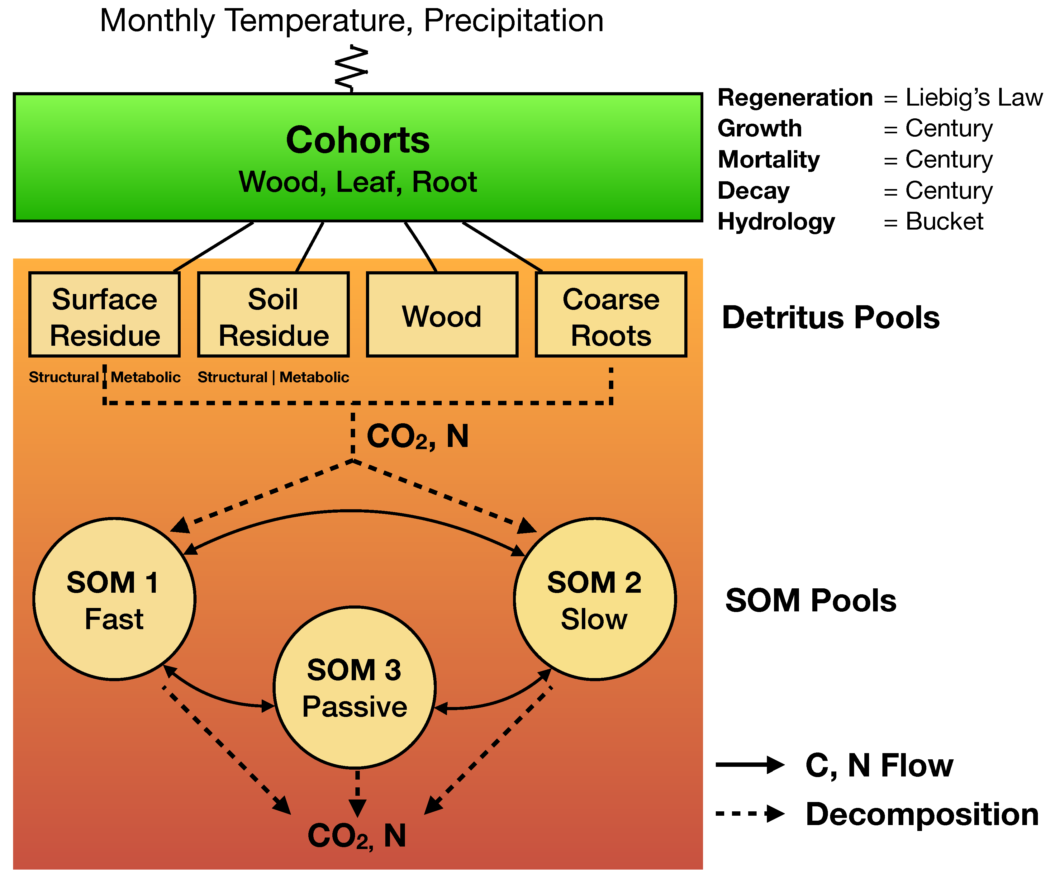
The Net Ecosystem Carbon and Nitrogen (NECN) model [101] is a simplified variant of the classical Century model [36,37]. The original ten soil layers in Century have been replaced by a single soil layer, with functions for growth and decay borrowed directly from Century v4.5. The NECN succession model Figure 1 is thus a process-based model that simulates C and N dynamics along the plant-soil continuum at a native monthly timestep.

Atmospheric effects are included through monthly climate (i.e., temperature maxima, minima, means, and standard deviations, and precipitation means and standard deviations). Explicit geometric representation of tree canopies is forgone in favor of bounded statistical growth models based theoretically on Liebig’s Law of the Minimum. Functions for growth, mortality, and decay are adopted from Century [36] while hydrology is based on the simple bucket model [102]. The regeneration function is the only new process in NECN and is also based on Liebig’s Law. For a detailed description of the NECN model, readers may refer to the original model publication [101]. Parameterization of the LANDIS-II model for both sites was based on updating parameters used in recent [103,104,105,106] and ongoing (Flanagan et al., in review) work.

2.1.2. PPA-SiBGC

The PPA-SiBGC model belongs to the SORTIE-PPA family of models [46,49] within the SAS-PPA model genre, based on a simple and analytically tractable approximation of the classical SORTIE gap model [107,108]. The Perfect Plasticity Approximation, or PPA [46,47], was derived from the dual assumptions of perfect crown plasticity (e.g., space-filling) and phototropism (e.g., stem-leaning), both of which were supported in empirical and modeling studies [49]. The discovery of the PPA was rooted in extensive observational and in silico research [46]. The PPA model was designed to overcome the most computationally challenging aspects of gap models in order to facilitate model scaling from the landscape to global scale.

The PPA and its predecessor, the size-and-age structured (SAS) equations [43,109], are popular model reduction techniques employed in current state-of-the-art terrestrial biosphere models [28]. The PPA model can be thought of metaphorically as Navier–Stokes equations of forest dynamics, capable of modeling individual tree population dynamics with a one-dimensional von Foerster partial differential equation [46]. The simple mathematical foundation of the PPA model is provided in Equation (1).

$${\displaystyle 1={\int }_{z^{*}}^{\infty }\sum _{j=1}^k{N}_j\left(z\right)A_j(z^{*},z)dz}$$

(1)

where k is the number of species, j is the species index, $N_j\left(z\right)$ is the density of species j at height z, $A_j(a^{*},z)$ is the projected crown area of species j at height z, and $dz$ is the derivative of height. In other words, we discard the spatial location of individual trees and calculate the height at which the integral of tree crown area is equal to the ground area of the stand. This height is known as the theoretical $z^{*}$ height, which segments trees into overstory and understory classes [46].

The segmentation of the forest canopy into understory and overstory layers allows for separate coefficients or functions for growth, mortality, and fecundity to be applied across strata, whose first moment accurately approximates the dynamics of individual-based forest models. Recent studies have shown that the PPA model faithfully reduces the dynamics of the more recent neighborhood dynamics (ND) SORTIE-ND gap model [110] and is capable of accurately capturing forest dynamics [111,112].

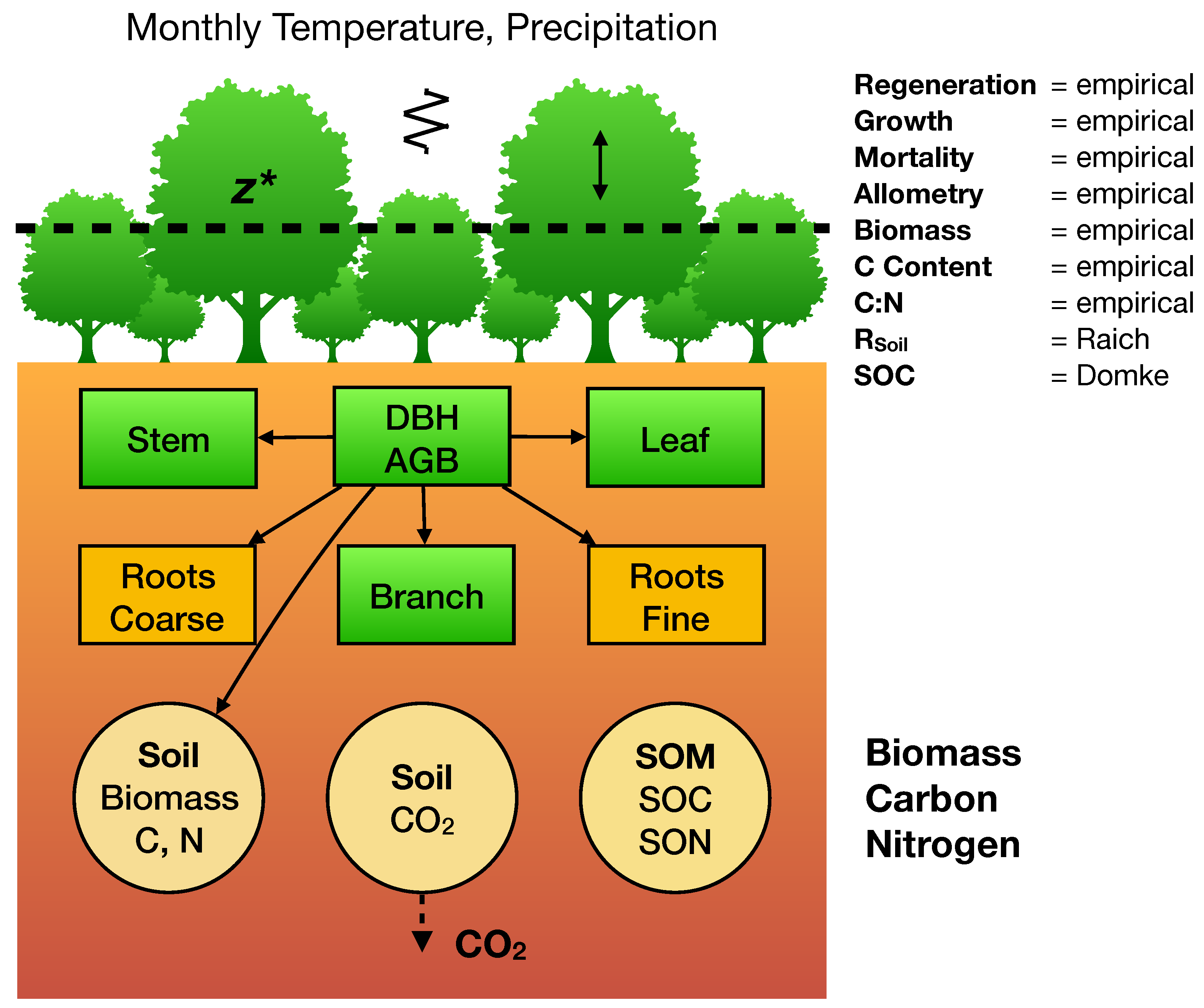
In this work, we applied a simple biogeochemistry variant of the SORTIE-PPA model, PPA-SiBGC (Erickson and Strigul, in review) Figure 2.

Empirical observations were relied upon for the C and N content of tree species compartments. Stoichiometric relations were used to estimate N from C, based on empirical measurements provided for both sites. All values were calculated directly from observations. Previously published equations [113] and parameters [114] were used to model crown allometry. Together with inventory data, general biomass equations were used to estimated dry weight mass ($kg$) for tree stems, branches, leaves, and, fine and coarse roots [115]. Carbon content was assumed to be 50% of dry mass, generally supported by data. Monthly soil respiration was modeled using the approach of Raich et al. [116], while soil organic C was modeled using the simple generalized approach of Domke et al. [117]. Species- and stratum-specific parameters for growth, mortality, and fecundity were calculated directly from field data for both sites. Net ecosystem exchange, or NEE, was modeled as $NEE={\mathrm{r}}_{\mathrm{soil}}-ANPP$ following previous studies, which note associated challenges in connecting field and flux tower measurements [118,119]. Here, ANPP, or annual net primary production, is the total site biomass increment adjusted for the C fraction. This is necessary given the current field-measurement basis of the PPA, which may be replaced by LiDAR measurements and/or process models in future work.

2.2. Site Descriptions

In the following sections, we describe the two forested sites on the East Coast of the United States: HF-EMS and the JERC-RD. A critical factor in the selection of the sites was the availability of eddy covariance flux tower data needed to validate NEE in the models.

2.2.1. HF-EMS

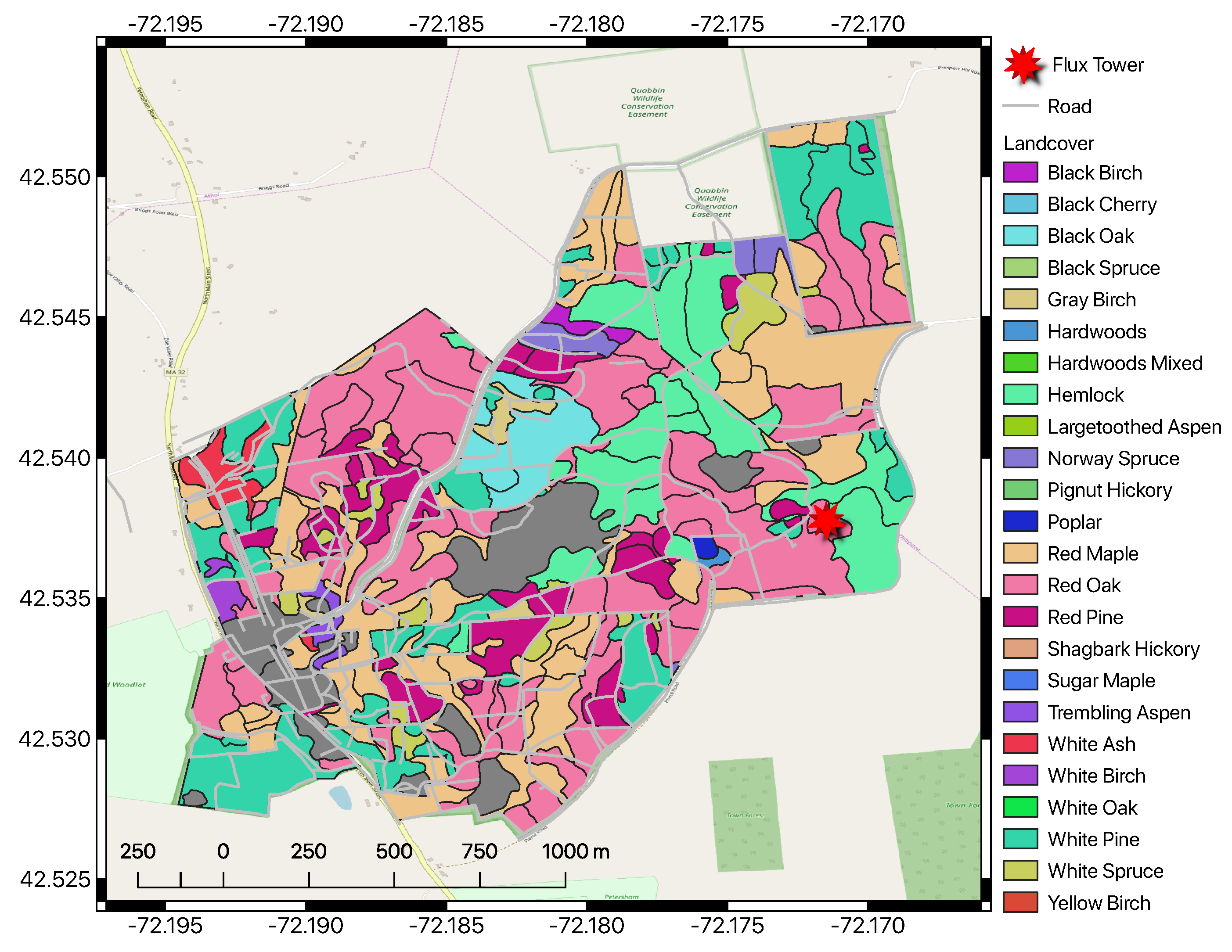
The HF-EMS EC flux tower is located within the Little Prospect Hill tract of Harvard Forest (42.538° N, 72.171° W, 340 m elevation) in Petersham, Massachusetts, approximately 100 km from the city of Boston [88]. A map of the site is shown in Figure 3. The tower has been recording NEE, heat, and meteorological measurements since 1989, with continuous measurements since 1991, making it the longest-running eddy covariance measurement system in the world. The site is currently predominantly deciduous broadleaf second-growth forests approximately 75–95 years in age, based on previous estimates [120]. Soils at Harvard Forest originate from sandy loam glacial till and are reported to be mildly acidic [88].

The site is dominated by red oak (Quercus rubra L.) and red maple (Acer rubrum L.) stands, with sporadic stands of Eastern hemlock (Tsuga canadensis (L.) Carrière), white pine (Pinus strobus L.), and red pine (Pinus resinosa Ait.). When the site was established, it contained 100 Mg C ${\mathrm{ha}}^{-1}$ in live aboveground woody biomass [120]. As noted by Urbanski et al. [88], approximately 33% of red oak stands were established prior to 1895, 33% prior to 1930, and 33% before 1940. A relatively hilly and undisturbed forest (since the 1930s) extends continuously for several ${\mathrm{km}}^2$ around the tower. In 2000, harvest operations removed 22.5 Mg C ${\mathrm{ha}}^{-1}$ of live aboveground woody biomass about 300 m S-SE from the tower, with little known effect on the flux tower measurements. The 40 biometric plots were designated via stratified random sampling within eight 500 m transects Urbanski et al. [88]. The HF-EMS tower site currently contains 34 biometric plots at 10 m radius each, covering 10,681 ${\mathrm{m}}^2$, or approximately one hectare, in area. Summary statistics for the EMS tower site for the year 2002 are provided in

Table 1. HF-EMS forest inventory summary for the 34 tower plots in 2002; DBH = depth at breast height (cm); BA = basal area per hectare (m${}^2$); Stocking = n${}_{trees}$ per hectare; QMD = quadratic mean diameter (cm); SDI = Reineke’s stand density index [121].

Statistic	N	Mean	St. Dev.	Min	Pctl(25)	Pctl(75)	Max
DBH${}_{Mean}$	34	24.64	3.50	17.32	22.39	27.13	31.97
DBH${}_{St.Dev.}$	34	10.92	2.74	6.11	8.60	12.51	16.88
BA	34	35.29	11.55	13.78	25.98	42.34	57.31
Stocking	34	639.43	232.38	318.31	421.76	787.82	1145.92
QMD	34	26.87	4.00	18.34	23.91	29.64	34.39
SDI	34	680.13	214.45	280.56	531.35	853.97	1071.37

.

A table of observed species abundances for the year 2002 are provided in

Table 2. HF-EMS species abundance for the 34 tower plots in 2002.

Species	Count
ACPE	56
ACRU	4924
BEAL	729
BELE	239
BEPO	116
CADE	1
FAGR	277
FRAM	258
ILVE	86
PIGL	397
PIRE	638
PIST	582
PRSE	270
QURU	2485
QUVE	247
TSCA	1926

, using tree species codes from the USDA PLANTS database (https://plants.usda.gov).

Previous research at the EMS EC flux tower site found unusually high rates of ecosystem respiration in winter and low rates in mid-to-late summer compared to other temperate forests [122]. While the mechanisms behind these observed patterns remains poorly understood, this observation is outside the scope of the presented research. Between 1992 and 2004, the site acted as a net carbon sink, with a mean annual uptake rate of 2.5 Mg C ha${}^{-1}$ year${}^{-1}$. Aging dominated the site characteristics, with a 101–115 Mg C ha${}^{-1}$ increase in biomass, comprised predominantly of growth of red oak (Quercus rubra). The year 1998 showed a sharp decline in net ecosystem exchange (NEE) and other metrics, recovering thereafter [88]. As Urbanski et al. [88] note of the Integrated Biosphere Simulator 2 (IBIS2) and similar models at the time, “the drivers of interannual and decadal changes in NEE are long-term increases in tree biomass, successional change in forest composition, and disturbance events, processes not well represented in current models.” The two models used in the intercomparison study, a SORTIE-PPA [46,47] variant and LANDIS-II with NECN succession [87,101], are intended to directly address these model shortcomings.

2.2.2. JERC-RD

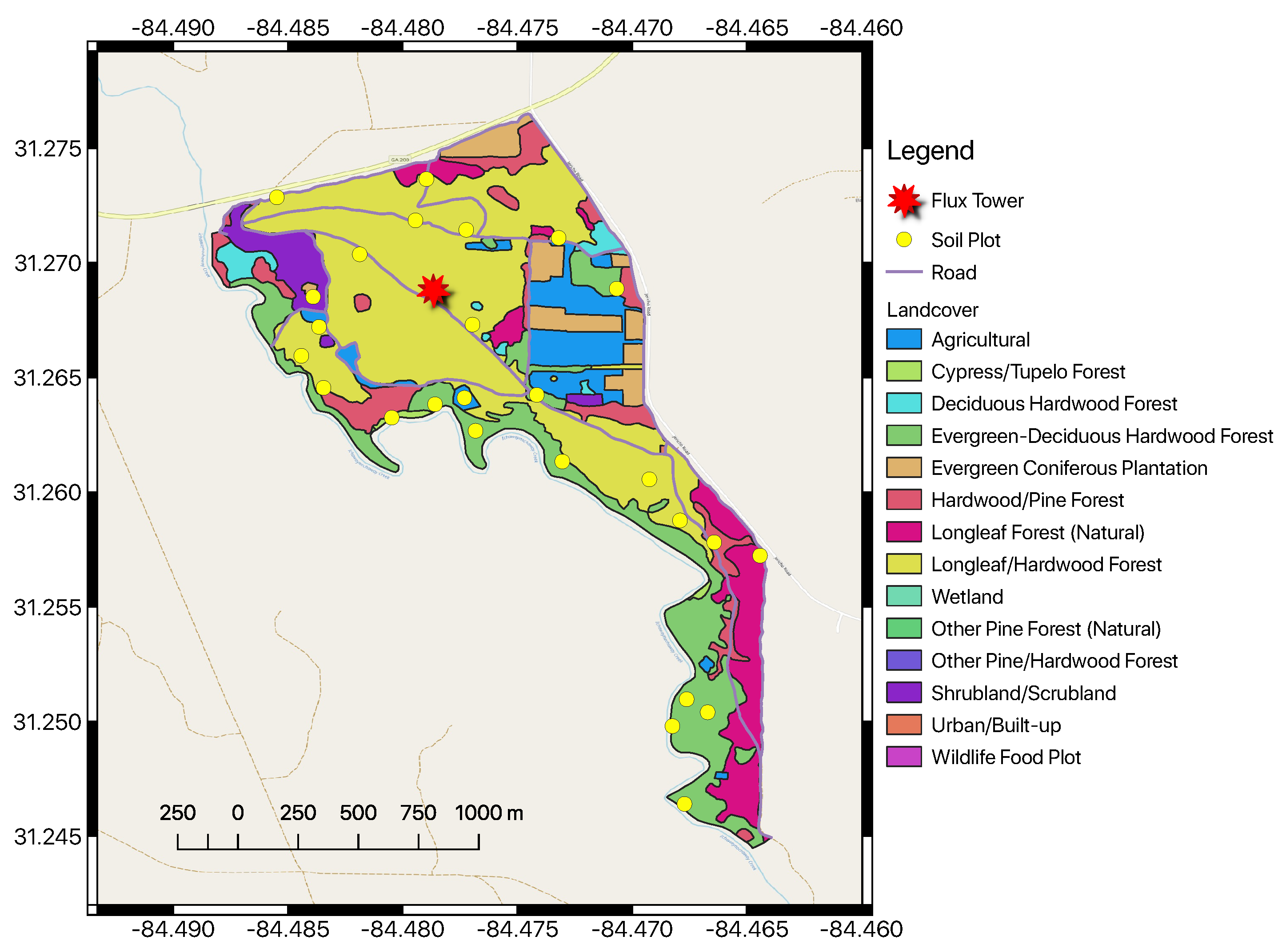
Jones Ecological Research Center at Ichauway is located near Newton, Georgia, USA (31° N, 84° W, 25–200 m elevation). A map of the JERC-RD flux tower with landcover classes is shown in Figure 4. The site falls within the East Gulf Coastal Plain and consists of flat to rolling land sloping to the southwest. The region is characterized by a humid subtropical climate with temperatures ranging from 5–34 °C and precipitation averaging 132 cm year${}^{-1}$. The overall site is 12,000 ha in area, 7500 ha of which are forested [123]. The site also exists within a tributary drainage basin that eventually empties into the Flint River. Soils here are underlain by karst Ocala limestone and mostly Typic Quartzipsamments, with sporadic Grossarenic and Aquic Arenic Paleudults [124]. Soils here often lack well-developed organic horizons [123,124,125].

Forests here are mostly second-growth, approximately 65–95 years in age. Long-leaf pine (Pinus palustris Mill.) dominates the overstory, while the understory is comprised primarily of wiregrass (Aristida stricta Michx.) and secondarily of shrubs, legumes, forbs, immature hardwoods, and regenerating long-leaf pine forests [126]. Prescribed fire is a regular component of management here, with stands often burned at regular 1–5 year intervals [123]. This has promoted wiregrass and legumes in the understory, while reducing the number of hardwoods [123]. The RD EC flux tower is contained within the mesic/intermediate sector. This site consists of only four primary tree species from two genera: Long-leaf pine (Pinus palustris), water oak (Quercus nigra L.), southern live oak (Quercus virginiana Mill.), and bluejack oak (Quercus incana W. Bartram). Measurements for the RD tower are available for the 2008–2013 time period. Summary statistics for the RD tower site for the year 2008 are provided in

Table 3. JERC-RD forest inventory summary for the four tower plots in 2009; DBH = depth at breast height (cm); BA = basal area per hectare (m${}^2$); Stocking = n${}_{trees}$ per hectare; QMD = quadratic mean diameter (cm); SDI = Reineke’s stand density index [121].

Statistic	N	Mean	St. Dev.	Min	Pctl(25)	Pctl(75)	Max
DBH${}_{Mean}$	4	31.498	2.870	27.426	30.530	33.392	33.719
DBH${}_{St.Dev.}$	4	12.733	2.737	10.525	11.293	13.285	16.714
BA	4	17.604	1.662	15.764	16.780	18.273	19.756
Stocking	4	201.000	60.871	164	170	205	292
QMD	4	33.968	3.374	29.350	32.665	35.987	37.152
SDI	4	310.965	39.514	278.001	291.255	318.514	368.254

.

A table of observed species abundances for the year 2009 are provided in

Table 4. JERC-RD species abundance for the four tower plots in 2009.

Species	Count
PIPA	2063
QUIN	14
QUNI	22
QUVI	66

.

Two recent studies [127,128] indicate that the mesic sector of this subtropical pine savanna functions as a moderate carbon sink (NEE = −0.83 Mg C ha${}^{-1}$year${}^{-1}$; −1.17 Mg C ha${}^{-1}$year${}^{-1}$), reduced to near-neutral uptake during the 2011 drought (NEE = −0.17 Mg C ha${}^{-1}$ year${}^{-1}$), and is a carbon source when prescribed burning is taken into account. NEE typically recovered to pre-fire rates within 30–60 days. The mechanisms behind soil respiration rates here again appear to be complex, site-specific, and poorly understood [128].

Overall, existing research highlights the importance of fire and drought to carbon exchange in long-leaf pine (Pinus palustris) and oak (Quercus spp.) savanna systems [127,128,129] at JERC. This is in contrast to the secondary growth-dominated deciduous broadleaf characteristics of Harvard Forest. Species diversity at the EMS tower site is 350% greater than that of the JERC-RD site, with 14 species from a variety of genera compared to four species from only two genera, Pinus and Quercus.

2.3. Site Data

Data collection methods may be accessed through the below data provider websites. Both sites provided a metadata file along with each data file, as is typically available to data users for the two sites. To conduct this model intercomparison exercise at HF-EMS, we leveraged the large amount of data openly available to the public through the Harvard Forest Data Archive:

http://harvardforest.fas.harvard.edu/harvard-forest-data-archive

Data were collected here for a range of studies, as evidenced by the Harvard Forest Data Archive. Datasets used in model validation include HF001-04, HF004-02, HF069-09, HF278-04, HF069-06, HF015-05, HF006-01, and HF069-13. These include weather station and forest inventory time-series, eddy covariance flux tower measurements, soil respiration, soil organic matter, and studies on C:N stoichiometry. Standard measurement techniques were used for each. For both sites, local tree species, age, depth-at-breast-height (DBH), biomass, soil, and meteorological data were primarily used to parameterize the models.

The Jones Ecological Research Center has hosted multiple research efforts over the years, collectively resulting in the collection of a large data library. However, JERC-RD site data are not made openly available to the public and are thus only available by request. One may find contact information located within their website:

http://www.jonesctr.org

Datasets used in model validation at JERC-RD include JC010-02, JC010-01, JC003-04, JC004-01, JC003-07, and JC011-01. These include weather station and eddy covariance flux tower measurements, forest inventory data, soil respiration, soil organic matter, and studies on C:N stoichiometry. Standard measurement techniques were also used for each of these.

2.4. Scales, Metrics, and Units

The selection of simulation years was based on the availability of EC flux tower data used in model validation. Thus, we simulated the HF-EMS site for the years 2002–2012 and the JERC-RD site for the years 2009–2013. For both sites and models, we initialized the model state in the first year of simulations using field observations. The PPA-SiBGC model used an annual timestep while LANDIS-II NECN used a monthly timestep internally. Both models may be set to other timesteps if desired.

The areal extent of the single-site model intercomparisons were designed to correspond to available field measurements. At both sites, tree inventories were conducted in 10,000 ${\mathrm{m}}^2$, or one-hectare, areas. All target metrics were converted to an annual areal basis to ease interpretation, comparison, and transferability of results. Importantly, an areal conversion will allow comparison to other sites around the world. While flux tower measurements for both sites were already provided on an areal (${\mathrm{m}}^{-2}$) basis, many other variables were converted to harmonize metrics between models and study sites. For example, moles ${\mathrm{CO}}_2$ measurements were converted to moles C through well-described molecular weights, all other measures of mass were converted to kg, and all areal and flux measurements were harmonized to ${\mathrm{m}}^{-2}$. A table of metrics and units used in the intercomparison of LANDIS-II and PPA-SiBGC is provided in

Table 5. Model intercomparison abbreviations, metrics, and units.

Abbreviation	Metric	Units
NEE	Net ecosystem exchange	kg C m${}^{-2}$year${}^{-1}$
$B_{AG}$	Aboveground biomass	kg mass m${}^{-2}$
$C_{AG}$	Aboveground C	kg C m${}^{-2}$
$N_{AG}$	Aboveground N	kg N m${}^{-2}$
$B_{BG}$	Belowground biomass	kg mass m${}^{-2}$
$C_{BG}$	Belowground C	kg C m${}^{-2}$
$N_{BG}$	Belowground N	kg N m${}^{-2}$
$C_{SO}$	Soil organic C	kg C m${}^{-2}$
$N_{SO}$	Soil organic N	kg N m${}^{-2}$
$r_{soil}$	Soil respiration C	kg C m${}^{-2}$year${}^{-1}$
ANPP	Aboveground net primary production	kg mass m${}^{-2}$year${}^{-1}$
$B_{Sp}$	Species aboveground biomass	kg mass m${}^{-2}$
$n_{Sp}$	Species relative abundance	%

.

In the subsequent section, we describe the model intercomparison methodology.

2.5. Model Intercomparison

Intercomparison of the PPA-SiBGC and LANDIS-II models at the HF-EMS and JERC-RD EC flux tower sites was conducted using a collection of object-oriented functional programming scripts written in the R language for statistical computing [83]. These scripts were designed to simplify model configuration, parameterization, operation, calibration/validation, plotting, and error calculation. The scripts and our parameters are available on GitHub (https://github.com/adam-erickson/ecosystem-model-comparison), making our results fully and efficiently reproducible. The directory structure of the repository is shown in Figure S1 in the Supplementary Materials. The R scripts are also designed to automatically load and parse the results from previous model simulations, in order to avoid reproducibility issues stemming from model stochasticity. We use standard regression metrics applied to the time-series of observation and simulation data to assess model fitness. The metrics used include the coefficient of determination ($R^2$), root mean squared error (RMSE), mean absolute error (MAE), and mean error (ME) or bias, calculated using simulated and observed values. Our implementation of $R^2$ follows the Bravais–Pearson interpretation as the squared correlation coefficient between observed and predicted values [130]. This implementation is provided in Equation (2).

$${\displaystyle R^2=r^2={\left(\frac{{\sum }_{i=1}^n(y_i-\overline{y})({\widehat{y}}_i-\overline{\widehat{y}})}{\sqrt{{\sum }_{i=1}^n{(y_i-\overline{y})}^2{({\widehat{y}}_i-\overline{\widehat{y}})}^2}}\right)}^2}$$

(2)

where n is the sample size, $y_i$ is the ith observed value, $\widehat{y_i}$ is the ith predicted value, $\overline{y}$ is the mean observed value, and $\overline{\widehat{y}}$ is the mean predicted value. The calculation of RMSE follows the standard formulation, as shown in Equation (3).

$${\displaystyle \mathrm{RMSE}=\sqrt{\frac{1}{n}\sum _{t=1}^n{e}_t^2}}$$

(3)

where n is the sample size and $e_t$ is the error for the tth value, or the difference between observed and predicted values. The calculation of MAE is similarly unexceptional, per Equation (4).

$${\displaystyle \mathrm{MAE}=\frac{1}{n}\sum _{t=1}^n\left|e_t\right|}$$

(4)

where again n is the sample size and $e_t$ is the error for the tth value. Our calculation of mean error (ME) or bias is the same as MAE, but without taking the absolute value.

While Nash–Sutcliffe efficiency (NSE) is often used in a simulation model context, we selected the Bravais–Pearson interpretation of $R^2$ over NSE to simplify the interpretation of results. The NSE metric replaces $1-(S{S}_{predictions}/S{S}_{observations})$ with $(S{S}_{observations}-S{S}_{predictions})/S{S}_{observations}$, where $SS$ is the sum of squares. Thus, NSE is analogous to the standard $R^2$ coefficient of determination used in regression analysis [131]. The implementation of $R^2$ that we selected is important to note, as its results are purely correlative and quantify only dispersion, ranging in value between zero and one. This has some desirable properties in that no negative or large values are produced, and that it is insensitive to differences in scale. Regardless of the correlation metric used, complementary metrics are needed to quantify the direction (i.e., bias) and/or magnitude of error. We rely on RMSE and MAE to provide information on error or residual magnitude, and ME to provide information on bias. We utilize a visual analysis to assess error directionality over time, as this can be poorly characterized by a single coefficient, masking periodicity.

We compute $R^2$, RMSE, MAE, and ME for time-series of the metrics described in Table 5 on page 13. These include NEE, above- and below-ground biomass, C, and N, soil organic C and N, soil respiration ($r_{soil}$), aboveground net primary production (ANPP), and, species aboveground biomass and relative abundance. All of these metrics are pools with the exception of NEE, $r_{soil}$, and ANPP fluxes. Finally, we diagnose the ability of both models to meet a range of logistical criteria related to deployment: Model usability, performance, and transferability. Model usability is assessed per four criteria:

• Ease of installation
• Ease of parameterization
• Ease of program operation
• Ease of parsing outputs

Model software performance is assessed per a single metric: The speed of program execution for each site for the predefined simulation duration. The durations are 11 years and five years for the HF-EMS and JERC-RD EC flux tower sites, respectively. Simulation results are output at annual temporal resolution, the standard resolution for both models, while NECN operates on a monthly timestep, and most other modules of LANDIS-II are annual. Finally, model transferability is assessed per the following five criteria:

• Model generalizability
• Availability of parameterization data
• Size of the program
• Cross-platform support
• Ease of training new users

Each of these logistical criteria are compared in a qualitative analysis, with the exception of software performance.

3. Results

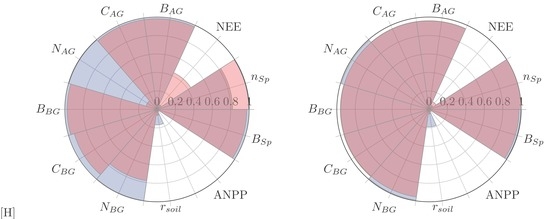
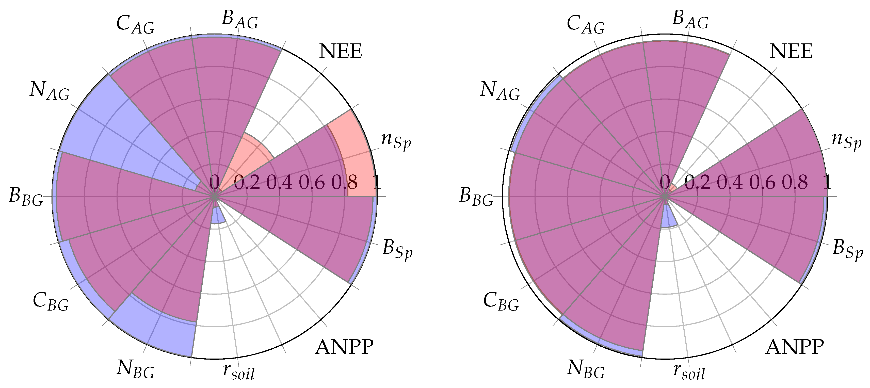
Both PPA-SiBGC and LANDIS-II NECN showed strong performance for pools at the two model intercomparison sites, frequently achieving $R^2$ values approaching unity. Yet, both models showed weak performance for fluxes. The models failed to accurately predict ANPP, while PPA-SiBGC showed stronger $r_{soil}$ performance and LANDIS-II NECN showed stronger NEE performance. The $R^2$ values for both models and sites are visualized in Figure 5.

On average, PPA-SiBGC outperformed LANDIS-II NECN across the sites and metrics tested, showing higher correlations, lower error, and less bias overall (HF-EMS $\overline{R^2}=0.73,+0.07$, $\overline{RMSE}=4.68,-9.96$, $\overline{ME}=-0.84,-5.96$; JERC-RD $\overline{R^2}=0.73,+0.01$, $\overline{RMSE}=2.18,-1.64$, $\overline{ME}=1.33,+1.03$). This result is based on calculating mean values for $R^2$, RMSE, MAE, and ME in order to clearly translate the overall results. The two models produced the following mean values for each of the four statistical metrics and two sites:

As shown in

Table 6. Overall mean values across each of the sites and metrics tested.

Metric	PPA-SiBGC				LANDIS-II NECN
	R${}^2$	RMSE	MAE	ME	R${}^2$	RMSE	MAE	ME
Mean	0.73	3.43	3.24	0.24	0.69	9.23	8.36	2.71

, PPA-SiBGC yielded higher $R^2$ values and lower RMSE, MAE, and ME values in comparison to LANDIS-II, on average, across all sites and metrics tested. Below, we provide model intercomparison results individually for the two sites, HF-EMS and JERC-RD.

3.1. HF-EMS

For the HF-EMS site, PPA-SiBGC showed higher $R^2$ values and lower RMSE, MAE, and ME values compared to LANDIS-II NECN across the range of metrics. While PPA-SiBGC predicted NEE and species relative abundance showed weaker correlations with observed values compared to LANDIS-II NECN, the magnitude of error was lower, as evidenced by lower RMSE, MAE, and ME values. While LANDIS-II NECN showed a lower magnitude of error for belowground N, this is the only metric where this is the case, while the correlation of this metric to observed values was also lower than that of PPA-SiBGC. Overall results for the HF-EMS site model intercomparison are shown in

Table 7. Model fitness for HF-EMS.

Metric	PPA-SiBGC				LANDIS-II NECN
	R${}^2$	RMSE	MAE	ME	R${}^2$	RMSE	MAE	ME
NEE	0.05	0.78	0.76	0.76	0.44	0.49	0.44	0.44
$B_{AG}$	1.00	10.31	10.30	10.30	0.98	2.48	2.48	−2.48
$C_{AG}$	1.00	0.05	0.05	0.05	0.98	1.24	1.24	−1.24
$N_{AG}$	1.00	1.44	1.44	−1.44	0.12	1.99	1.99	−1.99
$B_{BG}$	1.00	9.25	9.25	9.25	0.97	2.82	2.82	−2.82
$C_{BG}$	1.00	4.92	4.92	−4.92	0.94	6.99	6.99	−6.99
$N_{BG}$	1.00	0.56	0.56	0.56	0.78	0.12	0.12	−0.12
$r_{soil}$	0.17	0.63	0.62	−0.62	0.06	1.10	1.10	−1.10
ANPP	0.03	0.01	0.01	−0.01	0.0002	0.97	0.93	0.90
$C_{SO}$	...	26.49	26.49	−26.49	...	36.63	36.63	−36.63
$N_{SO}$	...	1.33	1.33	−1.33	...	1.60	1.60	−1.60
$B_{Sp}$	1.00	5.07	2.92	2.92	0.97	133.70	119.87	119.87
$n_{Sp}$	0.82	0.05	0.03	0	0.99	0.29	0.22	0.22
Mean	0.73	4.68	4.51	−0.84	0.66	14.65	13.57	5.11

.

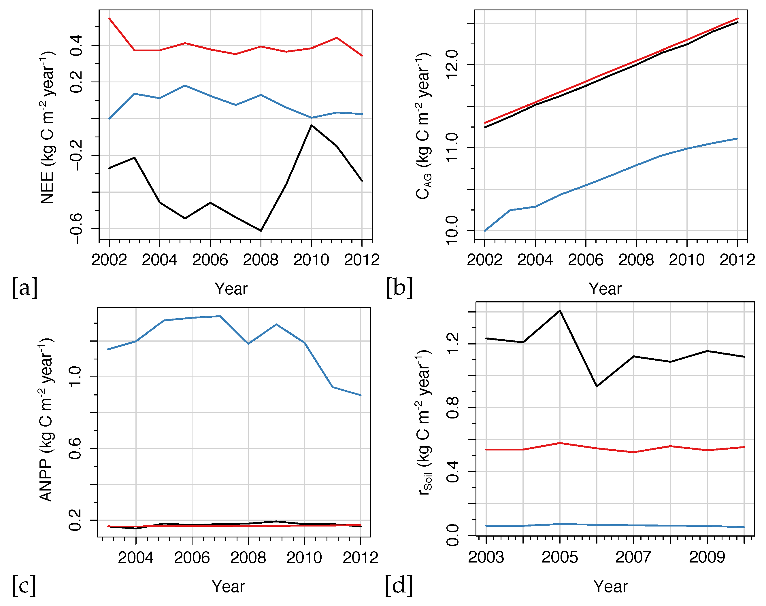
Time-series figures allow a visual analysis of the temporal dynamics between observations and model predictions in order to assess the ability of models to capture interannual variability in carbon exchange. Both models effectively captured integrals of dynamics in biomass, C, and, species biomass and abundance. In Figure 6, the temporal differences in modeled NEE, aboveground C, ANPP, and soil respiration are shown for the two models in comparison to observations for the HF-EMS site. LANDIS-II NECN predicted NEE showed a higher correlation with observations while the magnitude of error and bias were lower. Furthermore, LANDIS-II NECN predicted that the HF-EMS site is a net C source, rather than sink, in contrary to observations. Meanwhile, PPA-SiBGC outperformed LANDIS-II NECN in aboveground C per both $R^2$ and RMSE. Both models overpredicted species cohort biomass, while LANDIS-II NECN underpredicted total aboveground C.

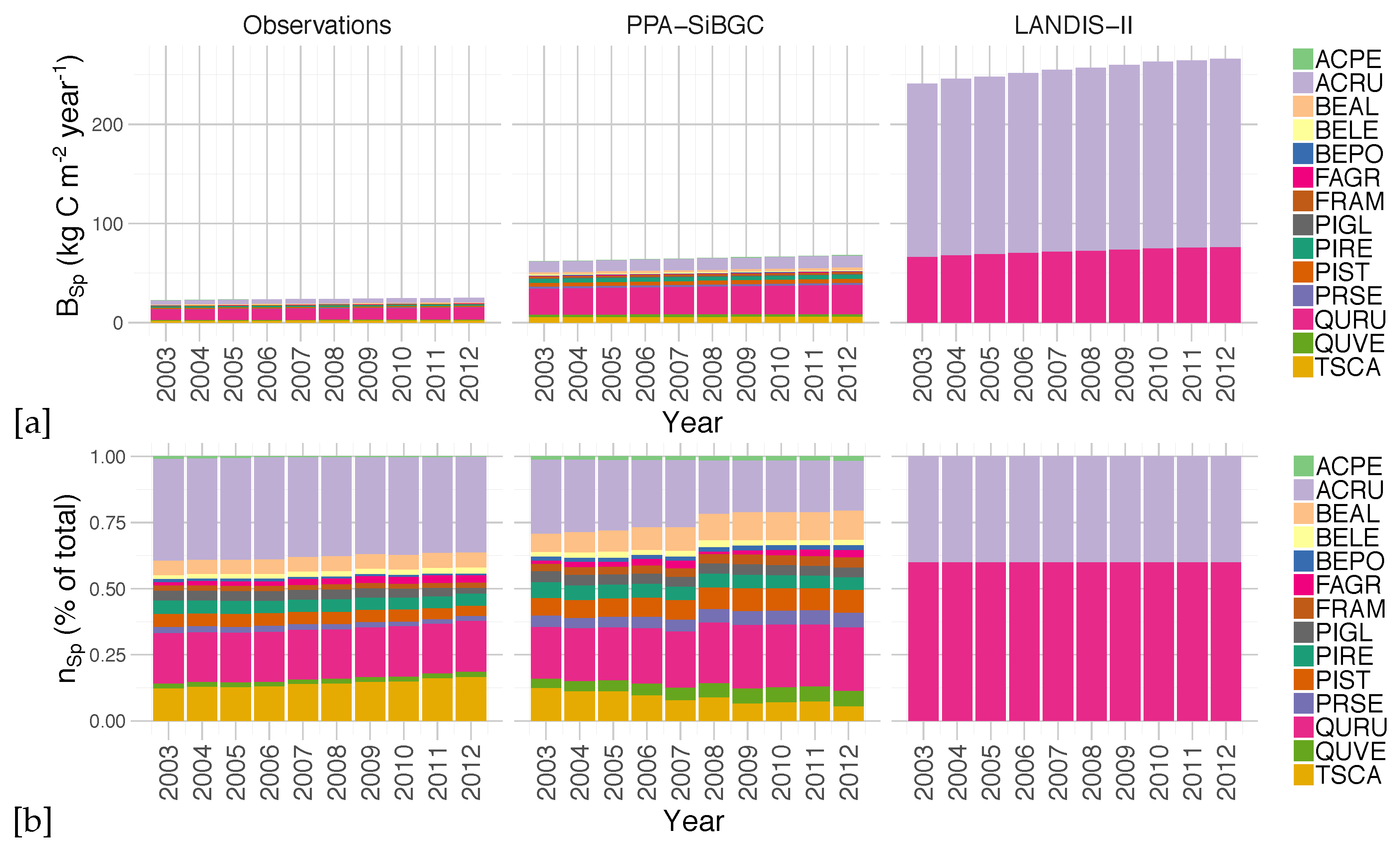
An analysis of simulated species biomass and abundance also shows greater fidelity of the PPA-SiBGC model to data, as shown in Figure 7. As LANDIS-II NECN does not contain data on individual trees, species relative abundance is calculated based on the number of cohorts of each species. Two species were simulated in LANDIS-II NECN, as there are no explicit trees in the model and the number of cohorts appears to have no effect on the total biomass. Results for PPA-SiBGC indicate that species relative abundance may be improved in future studies by optimizing mortality and fecundity rates. Meanwhile, species biomass predictions output by LANDIS-II NECN were inverted from those of the observations.

3.2. JERC-RD

For the JERC-RD site, both models showed stronger fidelity to data than for the HF-EMS site. Again, PPA-SiBGC showed higher $R^2$ values and lower RMSE and MAE values compared to LANDIS-II NECN across the range of metrics tested. Yet, the margin between models was smaller for the JERC RD site. While PPA-SiBGC demonstrated higher correlations and lower errors for most metrics tested, LANDIS-II NECN outperformed PPA-SiBGC in a few cases. This includes a higher correlation for NEE, ANPP, and lower magnitude of error for aboveground N, belowground biomass, soil respiration, and SOC. PPA-SiBGC, however, showed correlations equal or higher for all metrics tested, and lower errors for all other metrics. Overall results for the JERC-RD site model intercomparison are shown in

Table 8. Model fitness for JERC-RD.

Metric	PPA-SiBGC				LANDIS-II NECN
	R${}^2$	RMSE	MAE	ME	R${}^2$	RMSE	MAE	ME
NEE	0.05	0.12	0.11	0.05	0.09	0.13	0.11	−0.05
$B_{AG}$	0.96	1.48	1.47	1.47	0.96	9.77	9.76	−9.76
$C_{AG}$	0.96	1.63	1.63	−1.63	0.96	4.88	4.88	−4.88
$N_{AG}$	0.99	0.29	0.29	0.29	0.96	0.05	0.05	−0.05
$B_{BG}$	0.96	10.84	10.83	10.83	0.96	1.37	1.20	1.20
$C_{BG}$	0.96	0.25	0.25	0.25	0.96	0.96	0.95	−0.95
$N_{BG}$	0.99	1.44	1.44	−1.44	0.96	1.60	1.60	−1.60
$r_{soil}$	0.19	0.98	0.97	−0.97	0.05	0.90	0.90	−0.90
ANPP	0.00	0.12	0.10	−0.10	0.03	0.62	0.60	0.49
$C_{SO}$	...	4.30	4.30	4.30	...	0.17	0.17	−0.17
$N_{SO}$	...	0.38	0.38	0.38	...	0.12	0.12	0.12
$B_{Sp}$	1.00	6.47	3.90	3.90	0.98	28.97	20.52	20.52
$n_{Sp}$	1.00	0.02	0.01	0	1.00	0.09	0.09	−0.02
Mean	0.73	2.18	1.98	1.33	0.72	3.82	3.15	0.30

.

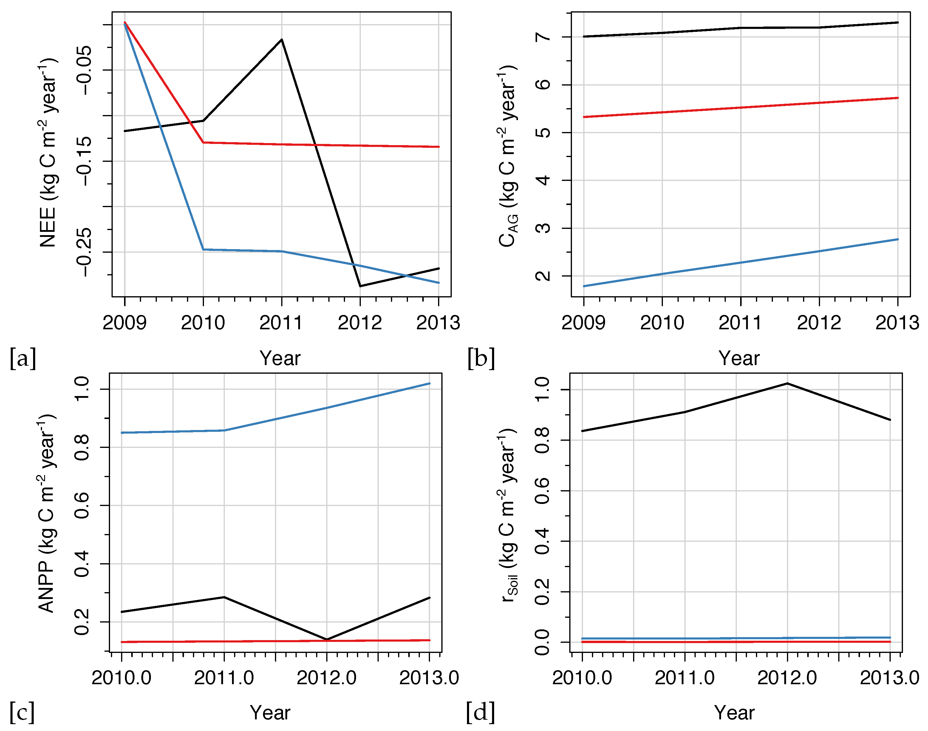
Time-series carbon exchange metrics for the JERC-RD site, presented in Figure 8, show that modeled NEE values are positively correlated with each other rather than with observed NEE, while the magnitude of error varies from favoring PPA-SiBGC to LANDIS-II NECN. Overall, the PPA-SiBGC model shows a lower magnitude of error for NEE, ANPP, and ${\mathrm{C}}_{\mathrm{AG}}$, and slightly higher for ${\mathrm{r}}_{\mathrm{soil}}$. Again, for ${\mathrm{r}}_{\mathrm{soil}}$ the two models show strong agreement, but underestimate observations by an order of magnitude. For ${\mathrm{C}}_{\mathrm{AG}}$ and ANPP, PPA-SiBGC shows good overall fit.

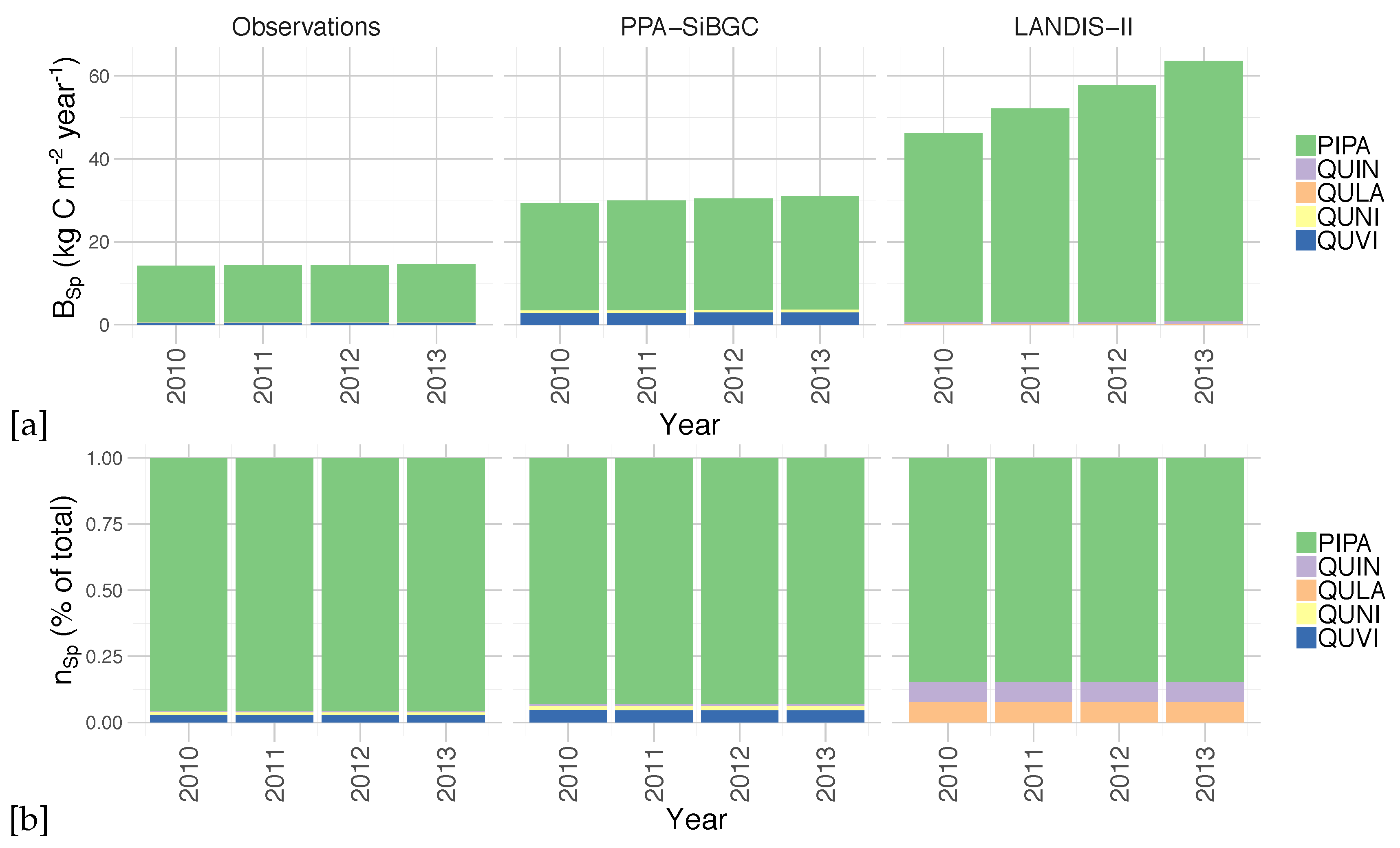
While both models showed higher performance at the JERC-RD site in comparison to the HF-EMS site, an analysis of simulated species biomass and abundance again indicates greater fidelity of the PPA-SiBGC model to data, as shown in Figure 9. While LANDIS-II NECN greatly overpredicts the rate of longleaf pine growth, PPA-SiBGC matches observed species abundance and biomass trajectories for all species present. While the correlations are high, PPA-SiBGC overpredicts the magnitude of species biomass.

Our results for the HF-EMS and JERC-RD site model intercomparison exercise show strong performance for both models at both sites. Results for the JERC-RD site are particularly close between the two models. Next, we assess results related to the logistics of model deployment to new computers, users, and modeling sites.

3.3. Model Usability, Performance, and Transferability

While the two models share a similar basis in forest dynamics and biogeochemistry modeling, they differ in important practical and conceptual terms. The command-line version of the PPA-SiBGC model used in this work, version 5.0, consists of approximately 500 lines of R code and is thus readily cross-platformed and portable. Meanwhile, the LANDIS-II model core and NECN succession extension are an estimated 2000 and 0.5 million lines of code, respectively. While this version of PPA-SiBGC fuses an explicit tree canopy geometry model with empirical data on fecundity, growth, mortality, and stoichiometry, the NECN extension of LANDIS-II borrows heavily from the process-based Century model [37], similar to the MAPSS-Century-1 (MC1) model [132]. This carries important implications for model parameterization needs. While PPA-SiBGC relies on typical forest inventory data, including tree species, age/size, and densities, LANDIS-II relies on species age/size and traits in the form of vital attributes, in addition to approximately 100 NECN parameters. Below, we summarize our findings regarding the logistics of model deployment.

3.3.1. Model Usability

In the following section, we provide an assessment of model usability based on four criteria.

• Ease of installation
  While LANDIS-II NECN requires the installation of two Windows programs, depending on the options desired, PPA-SiBGC is contained in a single R script and requires only a working R installation.
• Ease of parameterization
  While both models can be difficult to parameterize for regions with little to no observational data, the simple biogeochemistry in PPA-SiBGC requires an order of magnitude fewer parameters than LANDIS-II NECN. In addition, PPA-SiBGC uses commonly available forest inventory data while NECN requires a number of parameters that may be difficult to locate.
• Ease of program operation
  Both models use a command-line interface and are thus equally easy to operate. Yet, PPA-SiBGC is cross-platform and uses comma-separated-value (CSV) files for input tables, which are easier to work with than multiple tables nested within an unstructured text files. This additionally allows for simplification in designing model application programming interfaces (APIs), or model wrappers, a layer of abstraction above the models. These abstractions are important for simplifying model operation and reproducibility, and enable a number of research applications.
• Ease of parsing outputs
  All PPA-SiBGC outputs are provided in CSV files in a single folder while LANDIS-II NECN generates outputs in multiple formats in multiple folders. While the PPA-SiBGC format is simpler and easier to parse, the image output formats used by LANDIS-II carry considerable benefit for spatial applications. Both models may benefit by transitioning spatiotemporal data to the NetCDF scientific file format used by most general circulation and terrestrial biosphere models.

3.3.2. Model Performance

Next, we assess model performance in terms of the speed of operation on a consumer-off-the-shelf (COTS) laptop computer with a dual-core 2.8 GHz Intel Core i7-7600U CPU and 16 GB of DDR4-2400 RAM. We focus on a single performance metric, the timing of simulations. Other aspects of model performance in the form of precision and accuracy are described in previous sections. As shown in

Table 9. Simulation timing results.

Site	Model	Duration (years)	Elapsed (s)
HF-EMS	PPA-SiBGC	11	8.51
HF-EMS	LANDIS-II NECN	11	101.15
JERC-RD	PPA-SiBGC	5	2.25
JERC-RD	LANDIS-II NECN	5	61.51

, PPA-SiBGC was between 1200 and 2800% faster than LANDIS-II NECN in our timing tests. This was surprising given that PPA-SiBGC models true cohorts (i.e., individual trees) in an interpreted language while LANDIS-II models theoretical cohorts (i.e., cohorts without a physical basis) in a compiled language. The difference in speed is likely attributable to the parsimony of the PPA-SiBGC model.

3.3.3. Model Transferability

Here, we discuss model transferability. In this section, we assess the effort required to transfer the models to new locations, new computer systems, or new users. All three are important logistical criteria for effective model deployment.

• Model generalization
  Both models appear to generalize effectively to different forested regions of the world, as both have shown strong performance in this study and others. No clear winner is evident in this regard. In terms of model realism, PPA-SiBGC has a more realistic representation of forest canopies while LANDIS-II NECN has more realistic processes, as it is a Century model variant.
• Availability of parameterization data
  While LANDIS-II NECN requires substantially greater parameterization data compared to PPA-SiBGC, it may often be possible to rely on previously published parameters. Meanwhile, the growth, mortality, and fecundity parameters used by PPA-SiBGC are easy to calculate using common field inventory data. PPA-SiBGC is simpler to transfer in this regard given the wide availability of forest inventory data.
• Size of the program
  PPA-SiBGC is approximately 500 lines of R code, while LANDIS-II NECN is estimated at 0.5 million lines of C# code.
• Cross-platform support
  While Linux support may soon be supported with Microsoft .NET Core, LANDIS-II NECN is written in C# and is thus limited to Microsoft Windows platforms. Meanwhile, PPA-SiBGC is written in standard R code and is fully cross-platform.
• Ease of training new users
  While both models have a learning curve, the practical simplicity of PPA-SiBGC may make it easier to train new users. While LANDIS-II NECN contains more mechanistic processes and related parameters, these come at the cost of confusing new users. The model wrapper library we developed as part of this work vastly eases the operation of both models. Future studies should measure the time required for new users to effectively operate both models.

4. Discussion

First, it is important to clarify some terms used in this analysis. Gross primary production (GPP) is the net rate of carboxylation and oxygenation by RuBisCO and is calculated as $\mathrm{GPP}=P_g-R_p$, where $P_g$ is gross photosynthesis and $R_p$ is photorespiration. In EC flux data analyses, GPP is also known as gross ecosystem exchange (GEE) or gross ecosystem production (GEP) and is often estimated inversely from NEE or NEP flux tower retrievals as $\mathrm{GPP}=\mathrm{NEE}-R_e$, where $R_e$ is ecosystem respiration or the sum of auto- and heterotrophic respiration components. Thus, $R_e=R_m+R_g+R_h$ where $R_m$ is maintenance respiration, $R_g$ is autotrophic growth respiration, and $R_h$ is heterotrophic respiration. While GPP is the total amount of C fixed by plants in photosynthesis, NPP subtracts autotrophic respiration ($R_a$) as $\mathrm{NPP}=\mathrm{GPP}-R_a$ where $R_a=R_g+R_m$. NEE or net ecosystem production (NEP) is then calculated as NPP minus heterotrophic respiration, or $\mathrm{NEE}=\mathrm{NPP}-R_h$, which is equivalent to $\mathrm{NEE}=\mathrm{GPP}-R_e$. During the day, $\mathrm{NEE}=P_g+R_p+R_m+R_g+R_h$ while during the night, $P_g$ and $R_p$ are absent, making NEE approximate to ecosystem respiration, or $R_e$. Traditionally, gross or net exchange of ${\mathrm{CO}}_2$ into the forest is negative and fluxes into the atmosphere are positive, while each constituent process is discussed with a positive sign. Thus, NEE is often calculated as $\mathrm{NEE}=R_e-\mathrm{GPP}$ where each constituent flux term is always positive [133,134,135,136,137].

All this is to say that there exists much difficulty in relating NPP from field inventories and soil respiration samples directly to NEE from EC flux towers, integrated over the year. In our analyses, we assume that the observed annual biomass growth increment is equivalent to ANPP and that soil respiration ($r_{soil}$) is equivalent to ecosystem respiration ($R_e$), or $\mathrm{NEE}=\mathrm{NPP}-r_{soil}$. Yet, there are known error contributions at multiple conversion points, making the comparison of models based on field data and EC flux tower measurements difficult. For example, field inventory estimates of ANPP contain known sources of error in converting DBH to biomass, both above- and belowground [115], and there are additional errors in converting biomass to C based on a fixed fraction for each biomass compartment. Meanwhile, unlike $R_e$, $r_{soil}$ does not account for $R_g$ or $R_m$, only $R_h$. Even if these fluxes were approximately similar, spatial biases in the EC flux tower footprint or contributing area [138,139,140,141,142] may make field inventory and tower measurements difficult to harmonize.

As others have noted [118,119], including a previous study on flux measurements at the HF-EMS site [88], it is evident that treating ANPP as the C fraction of woody biomass increment per allometric relations from field data is a loose proxy for ecosystem ANPP, given its visible disconnection from observed NEE and ${\mathrm{r}}_{\mathrm{soil}}$ fluxes. Given the definition of NEE, the relation between these variables should be approximately linear. While others have reported hysteresis between peaks in NEE and growth increment at the HF-EMS site [88], we did not see evidence of this dynamic. Instead, flux tower NEE appears to have little to no connection to field data ANPP and observed ${\mathrm{r}}_{\mathrm{soil}}$ fluxes at both sites in this analysis. Nevertheless, both models showed good agreement with net changes to C and N pools. This may partially reflect difficulties in accounting for belowground processes, which can contribute disproportionately to C fluxes, and in connecting flux tower NEE to forest stands where the contributing area extent is far greater than a one-hectare stand, as is often the case [138,139,140].

This issue can be seen in Figure 6 and Figure 8. In this model intercomparison exercise, ANPP for the PPA-SiBGC model and field data are based on annual woody biomass increment, while ANPP in LANDIS-II NECN includes the Century process model for estimating ANPP. Rather than this basis making the NECN model purely process-based or mechanistic, species-specific growth is tightly constrained by empirical limits in a truncated logistic curve, with LAI and the number of cohorts present used as a proxy for growing space limitations and moisture and temperature used for physiological constraint based on Liebig’s Law of the Minimum. In contrast, PPA-SiBGC is parameterized with mean observed growth and mortality rates from field data, which vary depending on the canopy position of a cohort. Understory cohorts assumed to be in full shade face higher mortality and lower growth, as is widely evident in field data, while overstory cohorts assumed to be in full sunlight have higher growth and lower mortality rates. While soil and root processes are explicitly simulated in Century and thus LANDIS-II NECN, PPA-SiBGC relies on simple stoichiometric and allometric relations from field data to model these pools. In other words, PPA-SiBGC is designed primarily to model pools rater than fluxes, as the former are of generally higher interest to foresters.

The strong empirical basis of parameterization of both PPA-SiBGC and LANDIS-II NECN explains why the two models are often in better agreement with each other than with observations. The similarity of outputs from the two models is perhaps surprising, given their differences in model architecture and theoretical basis. This shows that, despite any mechanistic process present, both models in their current form are closely fit to field data and are therefore strongly empirical, as evidenced by their representation of growth processes. Meanwhile, this design choice limits the representation of fluxes in both models, as detailed process models are absent. This is expected for PPA-SiBGC, which is intended primarily to be a simple empirical pool model. This work also shows that observations between field and tower measurements are substantially disconnected. We estimate that fluxes are poorly represented by both models because they are tightly coupled to field inventory data rather than to tower-based measurements. Hence, patterns evident in field inventory data are reliably reproduced while fluxes appear wholly uncoupled.

The advancement of processor architectures has facilitated the development of increasingly complex forest models. Each new generation of processors allows researchers to conduct large-scale simulations faster and more efficiently than previous designs. As a result, forest models have grown into large, complex, analytically intractable programs. Rigorous intercomparison of models developed by different research groups, as well as the diagnosis of new versions of established models, is therefore a critical step in further advancing ecosystem models. This ensures that models are properly diagnosed and compared in a consistent, reliable, and transparent manner. Too often, model intercomparisons are conducted by each separate research group applying their own model in a manner that is, at best, inconsistent and opaque. In this work, we extended our model intercomparison by further providing wrapper functions that may be used to benchmark additional models or sites through a unified modeling framework. This ensures the consistency and transparency of intercomparison results.

The presented research is intended to establish the groundwork for future model intercomparison studies at both sites in order to advance the design of new models. Furthermore, we hope that this work will inspire a new generation of forest model intercomparisons in North America, which are sorely absent. Forest models have proven to be a critical testbed for improving the representation of vegetation dynamics in global terrestrial biosphere models [40,41,143], given the importance of forests in the global carbon cycle and the increased detail of local- to regional-scale models. Model benchmarking datasets and related results should be publicly shared and regularly updated with version-controlled software repositories (e.g., GitHub or GitLab), as is commonplace in the machine learning research community. Cloud computing providers may provide full reproducibility for cases where compute is limiting. In general, there is a broad disparity between modern software tools and existing forest models.

One important new forest model in development is a next-generation model from the SORTIE-PPA family of models, known as SORTIE-NG. This new model combines mechanistic representations of demographic processes, energetic and biogeochemical fluxes, and landscape disturbance dynamics, using hierarchical multiscale modeling with a modular component-based software framework [144]. Along with LM3-PPA [45], SORTIE-NG is among the first of a new class of hybrid models that we term ‘cohort-leaf’ models for their partitioning of energetic and biogeochemical fluxes amongst dynamic vegetation cohorts, instead of a single vertical ’big-leaf’ profile. The SORTIE-NG model includes evolutionary optimality principles as well as phenotype plasticity and intraspecific genetic diversity through first-class support for probabilistic modeling, borrowing design principles from probabilistic programming languages (e.g., [145]). Thus, SORTIE-NG is intended to be the first forest model to bridge the divide between big-leaf, gap, and landscape models, and to be designed from the outset as a probabilistic modeling framework [144]. Future model extensions are in the planning stages, including the first machine learning processes included in an ecosystem model.

While implemented in a ’close-to-metal’ language (i.e., C++17) and designed for efficiency, SORTIE-NG is more computationally demanding than the PPA-SiBGC model used in this paper. Yet, we anticipate that SORTIE-NG will be able to improved the fidelity to observed fluxes through reliance on detailed process models, which is the major shortcoming of both models considered in this paper. Similarly, there is a new version of the LANDIS-II NECN model in development known as NECN-Hydro, which remains a simplified variant of the Century model, but includes more detailed hydrological processes. The currently presented work provides not only an intercomparison of two current state-of-art models, but also open-source software and wrapper functions for simple and rapid comparison of our results with new models or sites. The selected forested ecosystems modeled in this work are among the best-studied model forests on Earth today. Specifically, the EMS EC flux tower at Harvard Forest is the longest running flux tower in the United States. Extensions of the presented work will allow rigorous model comparison methodologies for forest models that will benefit the research community at large.

Extensions of this work may also address the robustness of model predictions to variations in parameter values. The parameterization of complex forest biogeochemistry models such as LANDIS-II NECN and PPA-SiBGC is an important problem for consideration. Models such as LANDIS-II NECN operate with an order of magnitude more parameters than PPA-SiBGC, which can each be estimated with different levels of accuracy. Often, we know only the range of parameter values while parameterization can also depend on the statistical approach employed. Meanwhile, authors routinely employ additional model calibration that consists of adjusting parameters in order to obtain improved fitness, which we explicitly avoided in this study.

Conducting such analyses through a unified software framework in a fully transparent and reproducible manner is therefore of the utmost importance. This is exactly the type of analyses that our provided software is designed to support. In a parallel line of research, we extend this base-level implementation into a generic application programming interface (API) and toolkit for geoscientific simulation models, known as Erde [146], supporting both R and Python. The Erde framework provides machine learning model emulation, robust loss estimation, parameter optimization, probabilistic parameterization, samplers such as Latin hypercube sampling and Markov Chain Monte Carlo, and a number of other helper methods designed for complex simulation models. We utilize the Erde framework in the design of Erde Gym, a toolkit for developing and comparing optimization algorithms in the geosciences with a focus on reinforcement learning [146]. For the first time, Erde Gym will allow us to model systems (e.g., evolutionary plant optimality) as intelligent agents able to navigate complex environments.

4.1. Limitations

This study, similar to most other modeling studies, was limited by the availability, quality, and quantity of observational data. The lack of temporal depth in this data poses substantial challenges in modeling the long-term effects of forest succession, as these processes can operate on a century timescale or longer. However, diagnosing succession was not the aim of this study, as we instead focus on near-term validation of forest models using field measurements and EC flux tower data. Another limitation is that these methods may be challenging to implement for sites that are less well-characterized, particularly in the absence of EC flux tower data and/or tree species parameters. A combination of tower-based and remote sensing observations may help overcome this challenge in the coming years with advances in machine learning. In addition, the poor performance of both tested models in capturing fluxes and excellent performance in capturing stocks indicate that the two current models should be applied in cases where stocks, rather than fluxes, are of primary interest.

4.2. Future Opportunities

Future studies should expand upon the PPA with a first-principles representation of energetic and biogeochemical above- and below-ground processes in a modern component-based software framework. This work should fuse the new state-of-the-art forest biogeochemistry model with a model wrapper API written in R or Python, in order to expand native model functions to include Monte Carlo methods, machine-learning model emulation, robust loss functions, and optimization through a simple API enabling reproducibility. This would combine a high-performance forest model written in a compiled language with a simple, user-friendly interface written in an interpreted language, combining the best of both worlds. We are currently conducting work along this line by fusing the SORTIE-NG model with the Erde framework in order to develop state-of-the-art and user-friendly modeling capabilities, inspired by the design of modern deep learning frameworks such as PyTorch [147] and the Keras API [148].

In addition, there is a clear opportunity to link individual-based models such as PPA-SiBGC and SORTIE-NG to remote sensing data including airborne laser scanning or high-resolution multiview-stereo imagery (i.e., structure-from-motion), and hyperspectral indices of vegetation growth or stress. This line of work may assess opportunities for Bayesian data assimilation in addition to model parameterization and validation using detailed wall-to-wall forest structure maps. As models such as LES [32] provide more structural detail, spatially explicit data will be needed to parameterize the next generation of models. New data collection methods (e.g., [149]) will also be needed as the geometric realism of models advances toward the photorealistic detail offered by procedural models such as Lindenmayer- or L-systems [150,151].

5. Conclusions

In conclusion, the PPA-SiBGC and LANDIS-II NECN models represent vegetation dynamics previously absent in modeling studies at these sites. These include, “...long-term increases in tree biomass, successional change in forest composition, and disturbance events, processes not well represented in current models,” which drive interannual variation in NEE [88]. While the timescale of our simulations were decidedly short-term due to data limitations, both models showed good performance. While PPA-SiBGC showed stronger performance across the range of metrics tested, including the logistics of model deployment, LANDIS-II NECN also performed well across the metrics tested. Further studies are needed to compare more aspects of these and other models based on an array of performance criteria.

Ultimately, we hope that this study serves as the foundation for future forest ecosystem model intercomparisons for the North American continent, similar in spirit to the former TDE Ecosystem Model Intercomparison project [54]. This may help create the impetus for a Global Forest Model Intercomparison Project (ForestMIP) together with modeling groups on other continents. The aims of this research were not to determine which model is ’best’ for prognosis at two locations, but to improve the capabilities of existing models across a range of locations in order to advance earth system models. In this regard, there are beneficial aspects to both modeling approaches and the trade-offs presented largely depend on the desired application. Counter to the classical modeling trade-off of Levins [38], improvements in precision and generality resulted from realism.

References

1. von Carlowitz, H.C.; Bernigeroth, M. Sylvicultura Oeconomica Oder Haußwirthliche Nachricht und Naturmäßige Anweisung zur Wilden Baum-Zucht; Johann Friedrich Braun: Leipzig, Deutschland, 1713; p. 414. [Google Scholar]
2. Mikesell, M.W. The Deforestation of Mount Lebanon. Geogr. Rev. 1969, 59, 1–28. [Google Scholar] [CrossRef]
3. Hansman, J. Gilgamesh, Humbaba and the Land of the Erin-Trees. Iraq 1976, 38, 23–35. [Google Scholar] [CrossRef]
4. Holling, C.S. Resilience and Stability of Ecological Systems. Annu. Rev. Ecol. Syst. 1973, 4, 1–23. [Google Scholar] [CrossRef] [Green Version]
5. Levin, S.A. Ecosystems and the biosphere as complex adaptive systems. Ecosystems 1998, 1, 431–436. [Google Scholar] [CrossRef]
6. Vehkamäki, S. The concept of sustainability in modern times. In Sustainable Use of Renewable Natural Resources; Jalkanen, A., Nygren, P., Eds.; Helsingin Yliopiston Metsäekologian Laitoksen Julkaisuja, Helsingin Yliopisto, Metsäekologian Laitos: Helsinki, Finland, 2005; Chapter 2; pp. 23–35. [Google Scholar]
7. Rowe, J.S.; Scotter, G.W. Fire in the boreal forest. Quat. Res. 1973, 3, 444–464. [Google Scholar] [CrossRef]
8. Franklin, J.F.; Spies, T.A.; Pelt, R.V.; Carey, A.B.; Thornburgh, D.A.; Berg, D.R.; Lindenmayer, D.B.; Harmon, M.E.; Keeton, W.S.; Shaw, D.C.; et al. Disturbances and structural development of natural forest ecosystems with silvicultural implications, using Douglas-fir forests as an example. For. Ecol. Manag. 2002, 155, 399–423. [Google Scholar] [CrossRef]
9. Ripple, W.J.; Beschta, R.L. Restoring Yellowstone’s aspen with wolves. Biol. Conserv. 2007, 138, 514–519. [Google Scholar] [CrossRef]
10. Nitschke, C.R.; Innes, J.L. Integrating climate change into forest management in South-Central British Columbia: An assessment of landscape vulnerability and development of a climate-smart framework. For. Ecol. Manag. 2008, 256, 313–327. [Google Scholar] [CrossRef]
11. Erickson, A.M.; Nitschke, C.R.; Coops, N.C.; Cumming, S.G.; Stenhouse, G.B. Past-century decline in forest regeneration potential across a latitudinal and elevational gradient in Canada. Ecol. Model. 2015, 313, 94–102. [Google Scholar] [CrossRef]
12. Aitken, S.N.; Yeaman, S.; Holliday, J.A.; Wang, T.; Curtis-McLane, S. Adaptation, migration or extirpation: climate change outcomes for tree populations. Evolut. Appl. 2008, 1, 95–111. [Google Scholar] [CrossRef] [Green Version]
13. Aitken, S.N.; Whitlock, M.C. Assisted Gene Flow to Facilitate Local Adaptation to Climate Change. Annu. Rev. Ecol. Evolut. Syst. 2013, 44, 367–388. [Google Scholar] [CrossRef]
14. Erickson, A. Turing biocircuits for biosphere optimization. ResearchGate 2015. [Google Scholar] [CrossRef]
15. Attiwill, P.M. The disturbance of forest ecosystems: The ecological basis for conservative management. For. Ecol. Manag. 1994, 63, 247–300. [Google Scholar] [CrossRef]
16. Vuokila, Y. Functions for Variable Density Yield Tables of Pine Based on Temporary Sample Plots; Technical Report; Finnish Forest Research Institute: Helsinki, Finland, 1965. [Google Scholar]
17. Usher, M.B. A Matrix Approach to the Management of Renewable Resources, with Special Reference to Selection Forests. J. Appl. Ecol. 1966, 3, 355–367. [Google Scholar] [CrossRef]
18. Stage, A.R. Prognosis Model for Stand Development. Res. Pap. INT-RP-137; Technical Report; U.S. Dept. of Agriculture, Forest Service, Intermountain Forest and Range Experiment Station: Ogden, UT, USA, 1973. [Google Scholar]
19. Crookston, N.L.; Dixon, G.E. The forest vegetation simulator: A review of its structure, content, and applications. Comput. Electron. Agric. 2005, 49, 60–80. [Google Scholar] [CrossRef]
20. Bugmann, H.K.M. A Simplified Forest Model to Study Species Composition Along Climate Gradients. Ecology 1996, 77, 2055–2074. [Google Scholar] [CrossRef] [Green Version]
21. Keane, R.E.; Cary, G.J.; Davies, I.D.; Flannigan, M.D.; Gardner, R.H.; Lavorel, S.; Lenihan, J.M.; Li, C.; Rupp, T. A classification of landscape fire succession models: Spatial simulations of fire and vegetation dynamics. Ecol. Model. 2004, 179, 3–27. [Google Scholar] [CrossRef]
22. Mladenoff, D.J. LANDIS and forest landscape models. Ecol. Model. 2004, 180, 7–19. [Google Scholar] [CrossRef]
23. He, H.S. Forest landscape models: Definitions, characterization, and classification. For. Ecol. Manag. 2008, 254, 484–498. [Google Scholar] [CrossRef]
24. Xi, W.; Coulson, R.N.; Birt, A.G.; Shang, Z.B.; Waldron, J.D.; Lafon, C.W.; Cairns, D.M.; Tchakerian, M.D.; Klepzig, K.D. Review of forest landscape models: Types, methods, development and applications. Acta Ecol. Sin. 2009, 29, 69–78. [Google Scholar] [CrossRef]
25. Shifley, S.R.; He, H.S.; Lischke, H.; Wang, W.J.; Jin, W.; Gustafson, E.J.; Thompson, J.R.; Thompson, F.R.; Dijak, W.D.; Yang, J. The past and future of modeling forest dynamics: From growth and yield curves to forest landscape models. Landsc. Ecol. 2017, 32, 1307–1325. [Google Scholar] [CrossRef]
26. Sellers, P.J.; Mintz, Y.; Sud, Y.C.; Dalcher, A. A Simple Biosphere Model (SIB) for Use within General Circulation Models. J. Atmos. Sci. 1986, 43, 505–531. [Google Scholar] [CrossRef] [Green Version]
27. Fisher, J.B.; Huntzinger, D.N.; Schwalm, C.R.; Sitch, S. Modeling the Terrestrial Biosphere. Annu. Rev. Environ. Resour. 2014, 39, 91–123. [Google Scholar] [CrossRef]
28. Fisher, R.A.; Koven, C.D.; Anderegg, W.R.L.; Christoffersen, B.O.; Dietze, M.C.; Farrior, C.E.; Holm, J.A.; Hurtt, G.C.; Knox, R.G.; Lawrence, P.J.; et al. Vegetation demographics in Earth System Models: A review of progress and priorities. Glob. Chang. Biol. 2018, 24, 35–54. [Google Scholar] [CrossRef] [PubMed]
29. Kimmins, J.; Mailly, D.; Seely, B. Modelling forest ecosystem net primary production: the hybrid simulation approach used in forecast. Ecol. Model. 1999, 122, 195–224. [Google Scholar] [CrossRef]
30. Mäkelä, A.; Landsberg, J.; Ek, A.R.; Burk, T.E.; Ter-Mikaelian, M.; Ågren, G.I.; Oliver, C.D.; Puttonen, P. Process-based models for forest ecosystem management: current state of the art and challenges for practical implementation. Tree Physiol. 2000, 20, 289–298. [Google Scholar] [CrossRef] [PubMed] [Green Version]
31. Duursma, R.A.; Medlyn, B.E. MAESPA: A model to study interactions between water limitation, environmental drivers and vegetation function at tree and stand levels, with an example application to CO2 x drought interactions. Geosci. Model Dev. 2012, 5, 919–940. [Google Scholar] [CrossRef]
32. Liénard, J.; Strigul, N. An individual-based forest model links canopy dynamics and shade tolerances along a soil moisture gradient. R. Soc. Open Sci. 2016, 3, 150589. [Google Scholar] [CrossRef] [PubMed] [Green Version]
33. Landsberg, J.J.; Waring, R.H. A generalised model of forest productivity using simplified concepts of radiation-use efficiency, carbon balance and partitioning. For. Ecol. Manag. 1997, 95, 209–228. [Google Scholar] [CrossRef]
34. Farquhar, G.D.; von Caemmerer, S.; Berry, J.A. A biochemical model of photosynthetic CO2 assimilation in leaves of C3 species. Planta 1980, 149, 78–90. [Google Scholar] [CrossRef]
35. Sulman, B.N.; Moore, J.A.M.; Abramoff, R.; Averill, C.; Kivlin, S.; Georgiou, K.; Sridhar, B.; Hartman, M.D.; Wang, G.; Wieder, W.R.; et al. Multiple models and experiments underscore large uncertainty in soil carbon dynamics. Biogeochemistry 2018, 141, 109–123. [Google Scholar] [CrossRef]
36. Parton, W.J.; Anderson, D.W.; Cole, C.V.; Stewart, J.W.B. Simulation of organic matter formation and mineralization in semi-arid agroecosystems; Nutrient cycling in agricultural ecosystems. Special publication no. 23; The University of Georgia Press: Athens, GA, USA, 1983; pp. 533–550. [Google Scholar]
37. Parton, W.J.; Schimel, D.S.; Cole, C.V.; Ojima, D.S. Analysis of Factors Controlling Soil Organic Matter Levels in Great Plains Grasslands1. Soil Sci. Soc. Am. J. 1987, 51, 1173–1179. [Google Scholar] [CrossRef]
38. Levins, R. The Strategy of Model Building in Population Biology. Am. Sci. 1966, 54, 421–431. [Google Scholar]
39. Kimmins, H.; Blanco, J.A.; Seely, B.; Welham, C.; Scoullar, K. Forecasting Forest Futures: A Hybrid Modelling Approach to the Assessment of Sustainability of Forest Ecosystems and Their Values; Taylor & Francis Group: Boca Raton, FL, USA, 2010; p. 296. [Google Scholar]
40. Fisher, R.; McDowell, N.; Purves, D.; Moorcroft, P.; Sitch, S.; Cox, P.; Huntingford, C.; Meir, P.; Ian Woodward, F. Assessing uncertainties in a second-generation dynamic vegetation model caused by ecological scale limitations. New Phytol. 2010, 187, 666–681. [Google Scholar] [CrossRef] [PubMed] [Green Version]
41. Ahlström, A.; Xia, J.; Arneth, A.; Luo, Y.; Smith, B. Importance of vegetation dynamics for future terrestrial carbon cycling. Environ. Res. Lett. 2015, 10, 054019. [Google Scholar] [CrossRef] [Green Version]
42. Sitch, S.; Smith, B.; Prentice, I.C.; Arneth, A.; Bondeau, A.; Cramer, W.; Kaplan, J.O.; Levis, S.; Lucht, W.; Sykes, M.T.; et al. Evaluation of ecosystem dynamics, plant geography and terrestrial carbon cycling in the LPJ dynamic global vegetation model. Glob. Chang. Biol. 2003, 9, 161–185. [Google Scholar] [CrossRef]
43. Moorcroft, P.R.; Hurtt, G.C.; Pacala, S.W. A method for scaling vegetation dynamics: The ecosystem demography model (ED). Ecol. Monogr. 2001, 71, 557–586. [Google Scholar] [CrossRef]
44. Medvigy, D.; Wofsy, S.C.; Munger, J.W.; Hollinger, D.Y.; Moorcroft, P.R. Mechanistic scaling of ecosystem function and dynamics in space and time: Ecosystem Demography model version 2. J. Geophys. Res. Biogeosci. 2009, 114. [Google Scholar] [CrossRef] [Green Version]
45. Weng, E.S.; Malyshev, S.; Lichstein, J.W.; Farrior, C.E.; Dybzinski, R.; Zhang, T.; Shevliakova, E.; Pacala, S.W. Scaling from individual trees to forests in an Earth system modeling framework using a mathematically tractable model of height-structured competition. Biogeosciences 2015, 12, 2655–2694. [Google Scholar] [CrossRef]
46. Strigul, N.; Pristinski, D.; Purves, D.; Dushoff, J.; Pacala, S. Scaling from trees to forests: Tractable macroscopic equations for forest dynamics. Ecol. Monogr. 2008, 78, 523–545. [Google Scholar] [CrossRef]
47. Purves, D.W.; Lichstein, J.W.; Strigul, N.; Pacala, S.W. Predicting and understanding forest dynamics using a simple tractable model. Proc. Natl. Acad. Sci. USA 2008, 105, 17018–17022. [Google Scholar] [CrossRef] [PubMed] [Green Version]
48. Davis, A.V. Testing LANDIS-II to Stochastically Model Spatially Abstract Vegetation Trends in the Contiguous United States. Master’s Thesis, University of Southern California, Los Angeles, CA, USA, 2013. [Google Scholar]
49. Strigul, N. Individual-based models and scaling methods for ecological forestry: Implications of tree phenotypic plasticity. In Sustainable Forest Management; Garcia, J., Casero, J., Eds.; InTech: Rijeka, Croatia, 2012; pp. 359–384. [Google Scholar]
50. Seidl, R.; Rammer, W.; Scheller, R.M.; Spies, T.A. An individual-based process model to simulate landscape-scale forest ecosystem dynamics. Ecol. Model. 2012, 231, 87–100. [Google Scholar] [CrossRef] [Green Version]
51. Warszawski, L.; Frieler, K.; Huber, V.; Piontek, F.; Serdeczny, O.; Schewe, J. The Inter-Sectoral Impact Model Intercomparison Project (ISI–MIP): Project framework. Proc. Natl. Acad. Sci. USA 2014, 111, 3228–3232. [Google Scholar] [CrossRef] [PubMed]
52. Lischke, H.; Speich, M.; Schmatz, D.; Vacchiano, G.; Mairota, P.; Leronni, V.; Schuler, L.; Bugmann, H.; Bruna, J.; Thom, D.; et al. CoFoLaMo: Comparing forest landscape model simulations under different climate, interaction- and land use scenarios. EGU Gen. Assem. Conf. Abstr. 2016, 18, EPSC2016-13867. [Google Scholar]
53. Hanson, P.J.; Todd, D.E.; Huston, M.A.; Joslin, J.D.; Croker, J.L.; Auge, R.M. Description and Field Performance of the Walker Branch Throughfall Displacement Experiment: 1993–1996; Technical Report; Oak Ridge National Laboratory: Oak Ridge, TN, USA, 1998. [Google Scholar]
54. Hanson, P.J.; Amthor, J.S.; Wullschleger, S.D.; Wilson, K.B.; Grant, R.F.; Hartley, A.; Hui, D.; Hunt, E.R.; Johnson, D.W.; Kimball, J.S.; et al. Oak Forest Carbon and Water Simulations: Model Intercomparisons and Evaluations against Independent Data. Ecol. Monogr. 2004, 74, 443–489. [Google Scholar] [CrossRef]
55. Aber, J.D.; Ollinger, S.V.; Federer, C.A.; Reich, P.B.; Goulden, M.L.; Kicklighter, D.W.; Melillo, J.M.; Lathrop, R.G. Predicting the effects of climate change on water yield and forest production in the northeastern United States. Clim. Res. 1995, 5, 207–222. [Google Scholar] [CrossRef] [Green Version]
56. Williams, M.; Rastetter, E.B.; Fernandes, D.N.; Goulden, M.L.; Wofsy, S.C.; Shaver, G.R.; Melillo, J.M.; Munger, J.W.; Fan, S.M.; Nadelhoffer, K.J. Modelling the soil-plant-atmosphere continuum in a Quercus–Acer stand at Harvard Forest: The regulation of stomatal conductance by light, nitrogen and soil/plant hydraulic properties. Plant Cell Environ. 1996, 19, 911–927. [Google Scholar] [CrossRef]
57. Running, S.; Coughlan, J. A general model of forest ecosystem processes for regional applications I. Hydrologic balance, canopy gas exchange and primary production processes. Ecol. Model. 1988, 42, 125–154. [Google Scholar] [CrossRef] [Green Version]
58. Post, W.M.; Pastor, J. Linkages—An individual-based forest ecosystem model. Clim. Chang. 1996, 34, 253–261. [Google Scholar] [CrossRef]
59. Wang, Y.P.; Jarvis, P.G. Description and validation of an array model—MAESTRO. Agric. For. Meteorol. 1990, 51, 257–280. [Google Scholar] [CrossRef]
60. Warnant, P.; François, L.; Strivay, D.; Gérard, J.C. CARAIB: A global model of terrestrial biological productivity. Glob. Biogeochem. Cycles 1994, 8, 255–270. [Google Scholar] [CrossRef]
61. Tian, H.; Chen, G.; Zhang, C.; Liu, M.; Sun, G.; Chappelka, A.; Ren, W.; Xu, X.; Lu, C.; Pan, S.; et al. Century-Scale Responses of Ecosystem Carbon Storage and Flux to Multiple Environmental Changes in the Southern United States. Ecosystems 2012, 15, 674–694. [Google Scholar] [CrossRef] [Green Version]
62. Best, M.J.; Pryor, M.; Clark, D.B.; Rooney, G.G.; Essery, R.L.H.; Ménard, C.B.; Edwards, J.M.; Hendry, M.A.; Porson, A.; Gedney, N.; et al. The Joint UK Land Environment Simulator (JULES), model description—Part 1: Energy and water fluxes. Geosci. Model Dev. 2011, 4, 677–699. [Google Scholar] [CrossRef]
63. Clark, D.B.; Mercado, L.M.; Sitch, S.; Jones, C.D.; Gedney, N.; Best, M.J.; Pryor, M.; Rooney, G.G.; Essery, R.L.H.; Blyth, E.; et al. The Joint UK Land Environment Simulator (JULES), model description—Part 2: Carbon fluxes and vegetation dynamics. Geosci. Model Dev. 2011, 4, 701–722. [Google Scholar] [CrossRef]
64. Smith, B.; Wårlind, D.; Arneth, A.; Hickler, T.; Leadley, P.; Siltberg, J.; Zaehle, S. Implications of incorporating N cycling and N limitations on primary production in an individual-based dynamic vegetation model. Biogeosciences 2014, 11, 2027–2054. [Google Scholar] [CrossRef] [Green Version]
65. Bondeau, A.; Smith, P.C.; Zaehle, S.; Schaphoff, S.; Lucht, W.; Cramer, W.; Gerten, D.; Lotze-Campen, H.; Müller, C.; Reichstein, M.; et al. Modelling the role of agriculture for the 20th century global terrestrial carbon balance. Glob. Chang. Biol. 2007, 13, 679–706. [Google Scholar] [CrossRef]
66. Krinner, G.; Viovy, N.; de Noblet-Ducoudré, N.; Ogée, J.; Polcher, J.; Friedlingstein, P.; Ciais, P.; Sitch, S.; Prentice, I.C. A dynamic global vegetation model for studies of the coupled atmosphere-biosphere system. Glob. Biogeochem. Cycles 2005, 19. [Google Scholar] [CrossRef] [Green Version]
67. Zeng, N.; Qian, H.; Munoz, E.; Iacono, R. How strong is carbon cycle-climate feedback under global warming? Geophys. Res. Lett. 2004, 31. [Google Scholar] [CrossRef] [Green Version]
68. Inatomi, M.; Ito, A.; Ishijima, K.; Murayama, S. Greenhouse Gas Budget of a Cool-Temperate Deciduous Broad-Leaved Forest in Japan Estimated Using a Process-Based Model. Ecosystems 2010, 13, 472–483. [Google Scholar] [CrossRef]
69. Chang, J.; Ciais, P.; Wang, X.; Piao, S.; Asrar, G.; Betts, R.; Chevallier, F.; Dury, M.; François, L.; Frieler, K.; et al. Benchmarking carbon fluxes of the {ISIMIP}2a biome models. Environ. Res. Lett. 2017, 12, 45002. [Google Scholar] [CrossRef]
70. Frieler, K.; Lange, S.; Piontek, F.; Reyer, C.P.O.; Schewe, J.; Warszawski, L.; Zhao, F.; Chini, L.; Denvil, S.; Emanuel, K.; et al. Assessing the impacts of 1.5 °C global warming—Simulation protocol of the Inter-Sectoral Impact Model Intercomparison Project (ISIMIP2b). Geosci. Model Dev. 2017, 10, 4321–4345. [Google Scholar] [CrossRef]
71. Collalti, A.; Perugini, L.; Santini, M.; Chiti, T.; Nolè, A.; Matteucci, G.; Valentini, R. A process-based model to simulate growth in forests with complex structure: Evaluation and use of 3D-CMCC Forest Ecosystem Model in a deciduous forest in Central Italy. Ecol. Model. 2014, 272, 362–378. [Google Scholar] [CrossRef]
72. Collalti, A.; Marconi, S.; Ibrom, A.; Trotta, C.; Anav, A.; D’Andrea, E.; Matteucci, G.; Montagnani, L.; Gielen, B.; Mammarella, I.; et al. Validation of 3D-CMCC Forest Ecosystem Model (v.5.1) against eddy covariance data for 10 European forest sites. Geosci. Model Dev. 2016, 9, 479–504. [Google Scholar] [CrossRef] [Green Version]
73. Marconi, S.; Chiti, T.; Nolè, A.; Valentini, R.; Collalti, A. The Role of Respiration in Estimation of Net Carbon Cycle: Coupling Soil Carbon Dynamics and Canopy Turnover in a Novel Version of 3D-CMCC Forest Ecosystem Model. Forests 2017, 8, 220. [Google Scholar] [CrossRef]
74. Lasch, P.; Badeck, F.W.; Suckow, F.; Lindner, M.; Mohr, P. Model-based analysis of management alternatives at stand and regional level in Brandenburg (Germany). For. Ecol. Manag. 2005, 207, 59–74. [Google Scholar] [CrossRef]
75. Deckmyn, G.; Verbeeck, H.; de Beeck, M.O.; Vansteenkiste, D.; Steppe, K.; Ceulemans, R. ANAFORE: A stand-scale process-based forest model that includes wood tissue development and labile carbon storage in trees. Ecol. Model. 2008, 215, 345–368. [Google Scholar] [CrossRef]
76. Van Oijen, M.; Rougier, J.; Smith, R. Bayesian calibration of process-based forest models: Bridging the gap between models and data. Tree Physiol. 2005, 25, 915–927. [Google Scholar] [CrossRef]
77. Köhler, P.; Huth, A. The effects of tree species grouping in tropical rainforest modelling: Simulations with the individual-based model Formind. Ecol. Model. 1998, 109, 301–321. [Google Scholar] [CrossRef] [Green Version]
78. Loustau, D.; Bosc, A.; Colin, A.; Ogée, J.; Davi, H.; François, C.; Dufrêne, E.; Déqué, M.; Cloppet, E.; Arrouays, D.; et al. Modeling climate change effects on the potential production of French plains forests at the sub-regional level. Tree Physiol. 2005, 25, 813–823. [Google Scholar] [CrossRef] [Green Version]
79. Nadal-Sala, D.; Keenan, T.F.; Sabaté, S.; Gracia, C. Forest Eco-Physiological Models: Water Use and Carbon Sequestration BT—Managing Forest Ecosystems: The Challenge of Climate Change; Springer International Publishing: Berlin, Germany, 2017; pp. 81–102. [Google Scholar]
80. Haas, E.; Klatt, S.; Fröhlich, A.; Kraft, P.; Werner, C.; Kiese, R.; Grote, R.; Breuer, L.; Butterbach-Bahl, K. LandscapeDNDC: A process model for simulation of biosphere–atmosphere–hydrosphere exchange processes at site and regional scale. Landsc. Ecol. 2013, 28, 615–636. [Google Scholar] [CrossRef]
81. Gbondo-Tugbawa, S.S.; Driscoll, C.T.; Aber, J.D.; Likens, G.E. Evaluation of an integrated biogeochemical model (PnET-BGC) at a northern hardwood forest ecosystem. Water Resour. Res. 2001, 37, 1057–1070. [Google Scholar] [CrossRef] [Green Version]
82. Minunno, F.; Peltoniemi, M.; Launiainen, S.; Aurela, M.; Lindroth, A.; Lohila, A.; Mammarella, I.; Minkkinen, K.; Mäkelä, A. Calibration and validation of a semi-empirical flux ecosystem model for coniferous forests in the Boreal region. Ecol. Model. 2016, 341, 37–52. [Google Scholar] [CrossRef]
83. R Core Team. R: A Language and Environment for Statistical Computing; R Foundation for Statistical Computing: Vienna, Austria, 2018. [Google Scholar]
84. Schumacher, S.; Bugmann, H.; Mladenoff, D.J. Improving the formulation of tree growth and succession in a spatially explicit landscape model. Ecol. Model. 2004, 180, 175–194. [Google Scholar] [CrossRef]
85. Speich, M.; Lischke, H.; Scherstjanoi, M.; Zappa, M. FORHYCS—A coupled, spatially distributed eco-hydrological model for assessing climate and land use change impact in Switzerland at landscape scale. EGU Gen. Assem. Conf. Abstr. 2016, 18, EPSC2016-12988. [Google Scholar]
86. Lischke, H.; Zimmermann, N.E.; Bolliger, J.; Rickebusch, S.; Löffler, T.J. TreeMig: A forest-landscape model for simulating spatio-temporal patterns from stand to landscape scale. Ecol. Model. 2006, 199, 409–420. [Google Scholar] [CrossRef]
87. Scheller, R.M.; Domingo, J.B.; Sturtevant, B.R.; Williams, J.S.; Rudy, A.; Gustafson, E.J.; Mladenoff, D.J. Design, development, and application of LANDIS-II, a spatial landscape simulation model with flexible temporal and spatial resolution. Ecol. Model. 2007, 201, 409–419. [Google Scholar] [CrossRef]
88. Urbanski, S.; Barford, C.; Wofsy, S.; Kucharik, C.; Pyle, E.; Budney, J.; McKain, K.; Fitzjarrald, D.; Czikowsky, M.; Munger, J.W. Factors controlling CO2 exchange on timescales from hourly to decadal at Harvard Forest. J. Geophys. Res. Biogeosci. 2007, 112. [Google Scholar] [CrossRef]
89. Hawkins, D.M. The Problem of Overfitting. J. Chem. Inf. Comput. Sci. 2004, 44, 1–12. [Google Scholar] [CrossRef]
90. Mladenoff, D.J.; Host, G.E.; Boeder, J.; Crow, T.R. LANDIS: A model of forest landscape succession and management at multiple scales. In Proceedings of the Annual US Landscape Ecology Symposium, Oak Ridge, TN, USA, 24–27 March 1993; p. 77. [Google Scholar]
91. Mladenoff, D.J.; He, H.S. Design, behavior and application of LANDIS, an object-oriented model of forest landscape disturbance and succession. In Spatial Modeling of Forest Landscape Change: Approaches and Applications; Cambridge University Press: Cambridge, UK, 1999; pp. 125–162. [Google Scholar]
92. He, H.S.; Mladenoff, D.J.; Boeder, J. An object-oriented forest landscape model and its representation of tree species. Ecol. Model. 1999, 119, 1–19. [Google Scholar] [CrossRef]
93. Wang, W.J.; He, H.S.; Fraser, J.S.; Thompson, F.R.; Shifley, S.R.; Spetich, M.A. LANDIS PRO: A landscape model that predicts forest composition and structure changes at regional scales. Ecography 2014, 37, 225–229. [Google Scholar] [CrossRef]
94. Pennanen, J.; Kuuluvainen, T. A spatial simulation approach to natural forest landscape dynamics in boreal Fennoscandia. For. Ecol. Manag. 2002, 164, 157–175. [Google Scholar] [CrossRef]
95. Pennanen, J.; Greene, D.F.; Fortin, M.J.; Messier, C. Spatially explicit simulation of long-term boreal forest landscape dynamics: incorporating quantitative stand attributes. Ecol. Model. 2004, 180, 195–209. [Google Scholar] [CrossRef] [Green Version]
96. Roberts, D.W.; Betz, D.W. Simulating landscape vegetation dynamics of Bryce Canyon National Park with the vital attributes/fuzzy systems model VAFS/LANDSIM. In Spatial Modeling of Forest Landscape Change: Approaches and Applications; Cambridge University Press: Cambridge, UK, 1999; pp. 99–123. [Google Scholar]
97. Von Neumann, J.; Burks, A.W. Theory of self-reproducing automata. IEEE Trans. Neural Netw. 1966, 5, 3–14. [Google Scholar]
98. Noble, I.; Slatyer, R. The use of vital attributes to predict successional changes in plant communities subject to recurrent disturbances. Vegetatio 1980, 43, 5–21. [Google Scholar] [CrossRef]
99. Rothermel, R.C. A Mathematical Model for Predicting Fire Spread in Wildland Fuels. Res. Pap. INT-115; Technical Report; U.S. Department of Agriculture, Intermountain Forest and Range Experiment Station: Ogden, UT, USA, 1972. [Google Scholar]
100. ISO. ISO/IEC 14882:1998: Programming Languages — C++; ISO: Geneva, Switzerland, 1998; p. 732. [Google Scholar]
101. Scheller, R.M.; Hua, D.; Bolstad, P.V.; Birdsey, R.A.; Mladenoff, D.J. The effects of forest harvest intensity in combination with wind disturbance on carbon dynamics in Lake States Mesic Forests. Ecol. Model. 2011, 222, 144–153. [Google Scholar] [CrossRef]
102. Manabe, S. Climate and the Ocean Circulation. Mon. Weather Rev. 1969, 97, 739–774. [Google Scholar] [CrossRef]
103. Thompson, J.R.; Foster, D.R.; Scheller, R.; Kittredge, D. The influence of land use and climate change on forest biomass and composition in Massachusetts, USA. Ecol. Appl. Publ. Ecol. Soc. Am. 2011, 21, 2425–2444. [Google Scholar] [CrossRef] [Green Version]
104. Duveneck, M.J.; Thompson, J.R.; Gustafson, E.J.; Liang, Y.; de Bruijn, A.M.G. Recovery dynamics and climate change effects to future New England forests. Landsc. Ecol. 2017, 32, 1385–1397. [Google Scholar] [CrossRef]
105. Duveneck, M.J.; Scheller, R.M.; White, M.A.; Handler, S.D.; Ravenscroft, C. Climate change effects on northern Great Lake (USA) forests: A case for preserving diversity. Ecosphere 2014, 5, art23. [Google Scholar] [CrossRef]
106. Lucash, M.S.; Scheller, R.M.; Gustafson, E.J.; Sturtevant, B.R. Spatial resilience of forested landscapes under climate change and management. Landsc. Ecol. 2017, 32, 953–969. [Google Scholar] [CrossRef]
107. Pacala, S.W.; Canham, C.D.; Silander, J.A., Jr. Forest models defined by field measurements: I. The design of a northeastern forest simulator. Can. J. For. Res. 1993, 23, 1980–1988. [Google Scholar] [CrossRef]
108. Ribbens, E.; Silander, J.A.; Pacala, S.W. Seedling recruitment in forests: calibrating models to predict patterns of tree seedling dispersion. Ecology 1994, 75, 1794–1806. [Google Scholar] [CrossRef]
109. Hurtt, G.C.; Moorcroft, P.R.; And, S.W.P.; Levin, S.A. Terrestrial models and global change: Challenges for the future. Glob. Chang. Biol. 1998, 4, 581–590. [Google Scholar] [CrossRef]
110. Robbins, Z.; Scheller, R.; Case, B.; Strigul, N. The parameterization of PPA formulas using a SORTIE-ND Model for Harvard Forest. Abstracts of the AMS Spring Western Sectional Meeting. 2018. Available online: http://www.ams.org/amsmtgs/2248_abstracts/1137-92-206.pdf (accessed on 1 September 2018).
111. García, O. Can plasticity make spatial structure irrelevant in individual-tree models? For. Ecosyst. 2014, 1, 16. [Google Scholar] [CrossRef] [Green Version]
112. Lee, M.J.; García, O. Plasticity and extrapolation in modeling mixed-species stands. For. Sci. 2016, 62, 1–8. [Google Scholar] [CrossRef]
113. Canham, C.D.; Coates, K.D.; Bartemucci, P.; Quaglia, S. Measurement and modeling of spatially explicit variation in light transmission through interior cedar-hemlock forests of British Columbia. Can. J. For. Res. 1999, 29, 1775–1783. [Google Scholar] [CrossRef]
114. Case, B.S.; Buckley, H.L.; Barker-Plotkin, A.A.; Orwig, D.A.; Ellison, A.M. When a foundation crumbles: forecasting forest dynamics following the decline of the foundation species Tsuga canadensis. Ecosphere 2017, 8, e01893. [Google Scholar] [CrossRef] [Green Version]
115. Chojnacky, D.C.; Heath, L.S.; Jenkins, J.C. Updated generalized biomass equations for North American tree species. For. Int. J. For. Res. 2014, 87, 129–151. [Google Scholar] [CrossRef]
116. Raich, J.W.; Potter, C.S.; Bhagawati, D. Interannual variability in global soil respiration, 1980–94. Global Change Biology 2002, 8, 800–812. [Google Scholar] [CrossRef]
117. Domke, G.M.; Perry, C.H.; Walters, B.F.; Nave, L.E.; Woodall, C.W.; Swanston, C.W. Toward inventory-based estimates of soil organic carbon in forests of the United States. Ecol. Appl. 2017, 27, 1223–1235. [Google Scholar] [CrossRef]
118. Valentini, R.; De Angelis, P.; Matteucci, G.; Monaco, R.; Dore, S.; Mucnozza, G.E.S. Seasonal net carbon dioxide exchange of a beech forest with the atmosphere. Glob. Chang. Biol. 1996, 2, 199–207. [Google Scholar] [CrossRef]
119. Clark, D.a.; Brown, S.; Kicklighter, D.W.; Chambers, J.Q.; Thomlinson, J.R.; Ni, J. Measuring Net Primary Production in Forests: Concepts and Field Methods. Ecol. Appl. 2001, 11, 356–370. [Google Scholar] [CrossRef]
120. Barford, C.C.; Wofsy, S.C.; Goulden, M.L.; Munger, J.W.; Pyle, E.H.; Urbanski, S.P.; Hutyra, L.; Saleska, S.R.; Fitzjarrald, D.; Moore, K. Factors Controlling Long- and Short-Term Sequestration of Atmospheric CO2 in a Mid-latitude Forest. Science 2001, 294, 1688–1691. [Google Scholar] [CrossRef] [PubMed] [Green Version]
121. Reineke, L.H. Perfecting a stand-density index for even-aged forests. J. Agric. Res. 1933, 46, 627–638. [Google Scholar]
122. Giasson, M.A.; Ellison, A.M.; Bowden, R.D.; Crill, P.M.; Davidson, E.A.; Drake, J.E.; Frey, S.D.; Hadley, J.L.; et al. Soil respiration in a northeastern US temperate forest: A 22-year synthesis. Ecosphere 2013, 4, art140. [Google Scholar] [CrossRef]
123. Hendricks, J.J.; Hendrick, R.L.; Wilson, C.A.; Mitchell, R.J.; Pecot, S.D.; Guo, D. Assessing the patterns and controls of fine root dynamics: an empirical test and methodological review. J. Ecol. 2005, 94, 40–57. [Google Scholar] [CrossRef]
124. Drew, M.B.; Kirkman, L.K.; Angus, K. Gholson, J. The Vascular Flora of Ichauway, Baker County, Georgia: A Remnant Longleaf Pine/Wiregrass Ecosystem. Castanea 1998, 63, 1–24. [Google Scholar]
125. Goebel, P.C.; Hix, D.M. Changes in the composition and structure of mixed-oak, second-growth forest ecosystems during the understory reinitiation stage of stand development. Ecoscience 1997, 4, 327–339. [Google Scholar] [CrossRef]
126. Mitchell, R.J.; Kirkman, L.K.; Pecot, S.D.; Wilson, C.A.; Palik, B.J.; Boring, L.R. Patterns and controls of ecosystem function in longleaf pine—Wiregrass savannas. I. Aboveground net primary productivity. Can. J. For. Res. 1999, 29, 743–751. [Google Scholar] [CrossRef]
127. Whelan, A.; Mitchell, R.; Staudhammer, C.; Starr, G. Cyclic Occurrence of Fire and Its Role in Carbon Dynamics along an Edaphic Moisture Gradient in Longleaf Pine Ecosystems. PLoS ONE 2013, 8, e54045. [Google Scholar] [CrossRef]
128. Wiesner, S.; Staudhammer, C.L.; Loescher, H.W.; Baron-Lopez, A.; Boring, L.R.; Mitchell, R.J.; Starr, G. Interactions Among Abiotic Drivers, Disturbance and Gross Ecosystem Carbon Exchange on Soil Respiration from Subtropical Pine Savannas. Ecosystems 2018. [Google Scholar] [CrossRef]
129. Starr, G.; Staudhammer, C.L.; Loescher, H.W.; Mitchell, R.; Whelan, A.; Hiers, J.K.; O’Brien, J.J. Time series analysis of forest carbon dynamics: recovery of Pinus palustris physiology following a prescribed fire. New For. 2015, 46, 63–90. [Google Scholar] [CrossRef]
130. Krause, P.; Boyle, D.P.; Bäse, F. Comparison of different efficiency criteria for hydrological model assessment. Adv. Geosci. 2005, 5, 89–97. [Google Scholar] [CrossRef] [Green Version]
131. Nash, J.; Sutcliffe, J. River flow forecasting through conceptual models part I — A discussion of principles. J. Hydrol. 1970, 10, 282–290. [Google Scholar] [CrossRef]
132. Bachelet, D.; Lenihan, J.M.; Daly, C.; Neilson, R.P.; Ojima, D.S.; Parton, W.J. MC1: A dynamic vegetation model for estimating the distribution of vegetation and associated ecosystem fluxes of carbon, nutrients, and water. In Pacific Northwest Station General Technical Report PNW-GTR-508; USDA Forest Service: Corvallis, OR, USA, 2001. [Google Scholar]
133. Waring, R.H.; Law, B.E.; Goulden, M.L.; Bassow, S.L.; McCreight, R.W.; Wofsy, S.C.; Bazzaz, F.A. Scaling gross ecosystem production at Harvard Forest with remote sensing: A comparison of estimates from a constrained quantum-use efficiency model and eddy correlation. Plant Cell Environ. 1995, 18, 1201–1213. [Google Scholar] [CrossRef]
134. Goulden, M.L.; Daube, B.C.; Fan, S.M.; Sutton, D.J.; Bazzaz, A.; Munger, J.W.; Wofsy, S.C. Physiological responses of a black spruce forest to weather. J. Geophys. Res. Atmos. 1997, 102, 28987–28996. [Google Scholar] [CrossRef] [Green Version]
135. Law, B.E.; Waring, R.H.; Anthoni, P.M.; Aber, J.D. Measurements of gross and net ecosystem productivity and water vapour exchange of a Pinus ponderosa ecosystem, and an evaluation of two generalized models. Glob. Chang. Biol. 2000, 6, 155–168. [Google Scholar] [CrossRef]
136. Stoy, P.C.; Katul, G.G.; Siqueira, M.B.S.; Juang, J.Y.; Novick, K.A.; Uebelherr, J.M.; Oren, R. An evaluation of models for partitioning eddy covariance-measured net ecosystem exchange into photosynthesis and respiration. Agric. For. Meteorol. 2006, 141, 2–18. [Google Scholar] [CrossRef]
137. Piao, S.; Luyssaert, S.; Ciais, P.; Janssens, I.A.; Chen, A.; Cao, C.; Fang, J.; Friedlingstein, P.; Luo, Y.; Wang, S. Forest annual carbon cost: a global-scale analysis of autotrophic respiration. Ecology 2010, 91, 652–661. [Google Scholar] [CrossRef]
138. Foken, T.; Leclerc, M.Y. Methods and limitations in validation of footprint models. Agric. For. Meteorol. 2004, 127, 223–234. [Google Scholar] [CrossRef]
139. Sogachev, A.; Rannik, Ü.; Vesala, T. Flux footprints over complex terrain covered by heterogeneous forest. Agric. For. Meteorol. 2004, 127, 143–158. [Google Scholar] [CrossRef]
140. Kljun, N.; Calanca, P.; Rotach, M.W.; Schmid, H.P. A simple two-dimensional parameterisation for Flux Footprint Prediction (FFP). Geosci. Model Dev. 2015, 8, 3695–3713. [Google Scholar] [CrossRef] [Green Version]
141. Wang, H.; Jia, G.; Zhang, A.; Miao, C. Assessment of Spatial Representativeness of Eddy Covariance Flux Data from Flux Tower to Regional Grid. Remote Sens. 2016, 8, 742. [Google Scholar] [CrossRef]
142. Arriga, N.; Rannik, Ü.; Aubinet, M.; Carrara, A.; Vesala, T.; Papale, D. Experimental validation of footprint models for eddy covariance CO2 flux measurements above grassland by means of natural and artificial tracers. Agric. For. Meteorol. 2017, 242, 75–84. [Google Scholar] [CrossRef]
143. Friend, A.D.; Lucht, W.; Rademacher, T.T.; Keribin, R.; Betts, R.; Cadule, P.; Ciais, P.; Clark, D.B.; Dankers, R.; Falloon, P.D.; et al. Carbon residence time dominates uncertainty in terrestrial vegetation responses to future climate and atmospheric CO2. Proc. Natl Acad. Sci. USA 2014, 111, 3280–3285. [Google Scholar] [CrossRef] [PubMed]
144. Erickson, A.; Strigul, N. Design and Application of a Next-Generation Forest Biogeochemistry Model, Sortie-NG; ForestSAT 2018; Association for Forest Spatial Analysis Technologies: College Park, MD, USA, 2018. [Google Scholar]
145. Bingham, E.; Chen, J.P.; Jankowiak, M.; Obermeyer, F.; Pradhan, N.; Karaletsos, T.; Singh, R.; Szerlip, P.; Horsfall, P.; Goodman, N.D. Pyro: Deep Universal Probabilistic Programming. J. Mach. Learn. Res. 2018, arXiv:1810.09538. [Google Scholar]
146. Erickson, A.; Strigul, N. TBM Gym: A toolkit for developing and comparing terrestrial biosphere models and non-convex optimization algorithms. In AGU Fall Meeting 2018; American Geophysical Union: Washington, DC, USA, 2018. [Google Scholar]
147. Paszke, A.; Gross, S.; Chintala, S.; Chanan, G.; Yang, E.; DeVito, Z.; Lin, Z.; Desmaison, A.; Antiga, L.; Lerer, A. Automatic Differentiation in PyTorch. In Proceedings of the 31st Conference on Neural Information Processing Systems (NIPS 2017), Long Beach, CA, USA, 4–9 December 2017. [Google Scholar]
148. Chollet, F. Keras. 2015. Available online: https://keras.io (accessed on 1 September 2018).
149. Liénard, J.; Vogs, A.; Gatziolis, D.; Strigul, N. Embedded, real-time UAV control for improved, image-based 3D scene reconstruction. Measurement 2016, 81, 264–269. [Google Scholar] [CrossRef]
150. Lindenmayer, A. Mathematical models for cellular interactions in development II. Simple and branching filaments with two-sided inputs. J. Theor. Biol. 1968, 18, 300–315. [Google Scholar] [CrossRef]
151. Stava, O.; Pirk, S.; Kratt, J.; Chen, B.; Měch, R.; Deussen, O.; Benes, B. Inverse Procedural Modelling of Trees. Comput. Gr. Forum 2014, 33, 118–131. [Google Scholar] [CrossRef] [Green Version]
Figure 1. LANdscape DIsturbance and Succession II Net Ecosystem Carbon and Nitrogen (LANDIS-II NECN) model structure.
Forests 10 00180 g001
Figure 2. Perfect Plasticity Approximation with Simple Biogeochemistry (PPA-SiBGC) model structure; Raich et al. [116]; Domke et al. [117].
Forests 10 00180 g002
Figure 3. Harvard Forest (HF) EMS flux tower and landcover classes.
Forests 10 00180 g003
Figure 4. Jones Ecological Research Center (JERC) RD flux tower and landcover classes.
Forests 10 00180 g004
Figure 5. Overall model performance ( R 2 ) for both models and sites; left = HF-EMS; right = JERC-RD; periwinkle = PPA-SiBGC; pink = LANDIS-II NECN; violet = intersection.
Forests 10 00180 g005
Figure 6. Simulated and observed NEE, C AG , ANPP, and r Soil for the HF-EMS site; black = observations; red = PPA-SiBGC; blue = LANDIS-II NECN; (a) = NEE; (b) = C AG ; (c) = ANPP; (d) = r Soil .
Forests 10 00180 g006
Figure 7. HF-EMS: Simulated and observed species aboveground biomass and relative abundance; (a) = biomass; (b) = abundance; left = observations, middle = PPA-SiBGC, right = LANDIS-II NECN; note that different scales are used for biomass.
Forests 10 00180 g007
Figure 8. Simulated and observed NEE, C AG , ANPP, and r Soil for the JERC-RD site; black = observations; red = PPA-SiBGC; blue = LANDIS-II NECN; (a) = NEE; (b) = C AG ; (c) = ANPP; (d) = r Soil .
Forests 10 00180 g008
Figure 9. JERC-RD: Simulated and observed species aboveground biomass and relative abundance; (a) = biomass; (b) = abundance; left = observations, middle = PPA-SiBGC, right = LANDIS-II NECN; note that different scales are used for biomass.
Forests 10 00180 g009