Article

Time-Series Forecasting of Seasonal Data Using Machine Learning Methods

Department of Informatics and Control in Technical Systems, Sevastopol State University, 299053 Sevastopol, Russia
*
Author to whom correspondence should be addressed.
Algorithms 2023, 16(5), 248; https://doi.org/10.3390/a16050248
Submission received: 20 February 2023 / Revised: 30 April 2023 / Accepted: 8 May 2023 / Published: 10 May 2023
(This article belongs to the Special Issue Machine Learning for Time Series Analysis)

Abstract

:
The models for forecasting time series with seasonal variability can be used to build automatic real-time control systems. For example, predicting the water flowing in a wastewater treatment plant can be used to calculate the optimal electricity consumption. The article describes a performance analysis of various machine learning methods (SARIMA, Holt-Winters Exponential Smoothing, ETS, Facebook Prophet, XGBoost, and Long Short-Term Memory) and data-preprocessing algorithms implemented in Python. The general methodology of model building and the requirements of the input data sets are described. All models use actual data from sensors of the monitoring system. The novelty of this work is in an approach that allows using limited history data sets to obtain predictions with reasonable accuracy. The implemented algorithms made it possible to achieve an R-Squared accuracy of more than 0.95. The forecasting calculation time is minimized, which can be used to run the algorithm in real-time control and embedded systems.

1. Introduction

Generally, a time series is a set of data ordered in time. Each time series element is assigned a unique Timestamp T S index. The distance between indexes can be seconds, hours, days, months, or even years. At that time, the value of the time interval between neighboring indexes is usually assumed to be the same and is denoted by T s = T S k T S k 1 . For example, the change in quotes on the exchange can be described by the set of real numbers Y k with an interval with T s = 1 min, and the quotes are accumulated in the data set from the start of trading on the exchange until its closure. Some finite sample Y is considered at a specific time interval t t 0 , t 0 + T s ,   , t f . In general, a time series can be represented by a function of the form Y t = T t + S t + R t , where T t is the trend cycle component (Trend), S t is the seasonal component (Seasonal), and R t are the residuals (Residuals). Time series containing a seasonal component S t has periodicity properties. That is, the character of the variability of the time series repeats from time to time. An example is the growth of purchasing power during the holiday season or the growth of passenger traffic during the vacation season. Modern machine learning methods can create predictive models for this type of time series, which allows calculating the estimate (forecasting) of the parameter for several steps forward relative to the current point in time (forecast horizon) [1,2,3,4,5,6]. In this case, to train the model, we need only knowledge of the history of the parameter, which is described by the time series, that is, the historical data on the time interval, the length of which corresponds to several periods of seasonal variability T . The knowledge of other parameters, as a rule, is not required. Thus, the task arises of building models which can estimate some experimental parameters with seasonal variability on some forecast horizon based on information about previous and present values of this parameter (historical data). Currently, the analysis and forecasting of time series with seasonal variability are most common in financial markets and trading [7,8,9,10]. The works [11,12,13,14] build models to obtain forecasts of commodity prices and rates of cryptocurrencies. The works [15,16] forecast the value of tourist flow, depending on the time of year. In turn, tourist flows impact changes in passenger traffic by various modes of transport, as shown in [17,18]. Processes that affect climate [19,20], ecology [21,22], and medicine [23,24] are also subject to seasonal changes. The authors [25,26,27,28] describe the application of time series with seasonal variability in industry and energy and resource consumption. The application of deep learning technology and long short-term memory network for physical systems is shown in [29,30]. All research above uses practically the same set of methods and algorithms. First, these are methods for obtaining autoregressive models ARIMA (Autoregressive Integrated Moving Average) and SARIMA (Seasonal ARIMA), which have been known for quite a long time, and the mathematical apparatus of which is well developed. The first mention of the method was made in 1970 by George Box and Gwilym Jenkins. ARIMA/SARIMA allows us to obtain the primary class of models used for time series analysis and forecasting. The Holt-Winters Exponential Smoothing method, developed by Charles Holt in the late 1950s, and its modern modification, the Exponential Smoothing Algorithm (ETS), are also used. In addition to the above methods, which can already be classified as classical, new algorithms have appeared in recent years, successfully coping with constructing predictive models of time series with seasonal variability. These are the methods of Facebook Prophet [31], XGboost [32], and a set of Artificial Neural Network (ANN) methods, in particular, the Long Term Memory (LSTM) method [33,34,35].
This article presents the results of applying the above methods to build a model to predict the inlet flow of wastewater from a wastewater treatment plant. This model can be used to calculate the optimal loading of equipment and to ensure a given quality of treatment, which in turn will significantly reduce the consumption of electrical energy by the plant. The methodology of data preparation and the specifics of applying each of the methods are described, the statistical analysis of the obtained results is performed, and recommendations for improving the forecast quality are given. All numerical calculations and implementation of algorithms were performed using the Python language and specialized libraries [36]. The novelty of the work lies in the use of machine learning methods for predicting the technological process. The forecast results are used in the real-time control system. A method for preparing data for use in predictive models is proposed. A feature of the approach is using data over a short time interval. A sample for the last 15–17 days is used for training. In this case, the forecast is made for the next two days. Automatic retraining of the model is used every 24 h to maintain accuracy of the model. At the same time, it takes less than 10 s to train a new model, and the accuracy of the model remains unchanged. As a result, several methods were chosen that optimally solve the problem. The developed algorithms can be easily integrated into embedded control systems or software tools for real-time treatment plant control and do not require significant computing resources.
The Section 2 describes the main approaches used for data preprocessing. The data format is defined, and a technical map is proposed for solving the problem. The Section 3 discusses the main provisions of the methods and provides recommendations for using Python libraries. The graphical results of checking each model on a test data set are also given. For the XGBoost and LTSM methods, an algorithm for generating a synthetic data set for training is given, which must be obtained from the original data set to build a prediction model. The Section 4 describes the statistical metrics used to compare the accuracy of the models. The results of the numerical calculation of the metrics are given, as well as the time spent on the preparation and use of each model. The Section 5 summarizes the findings and outlines areas for further research.

2. Methodology

The study aimed to find, using known approaches, the optimal algorithm that would allow building a short-term forecast in the shortest time and with the least initial dataset (historical data).
The main idea and novelty of the implemented approach are that our algorithm does not use the same machine-learning model. The model is built again using new data every 24 h. That is why short-term samples of initial data are used for training and testing models. This idea allows us to consider new factors that cannot be included in the long-term model, such as equipment replacement, maintenance, and unplanned load changes. It keeps the forecast accuracy at a high level, as well.
Below is a methodology that allows us to implement the described approach effectively.

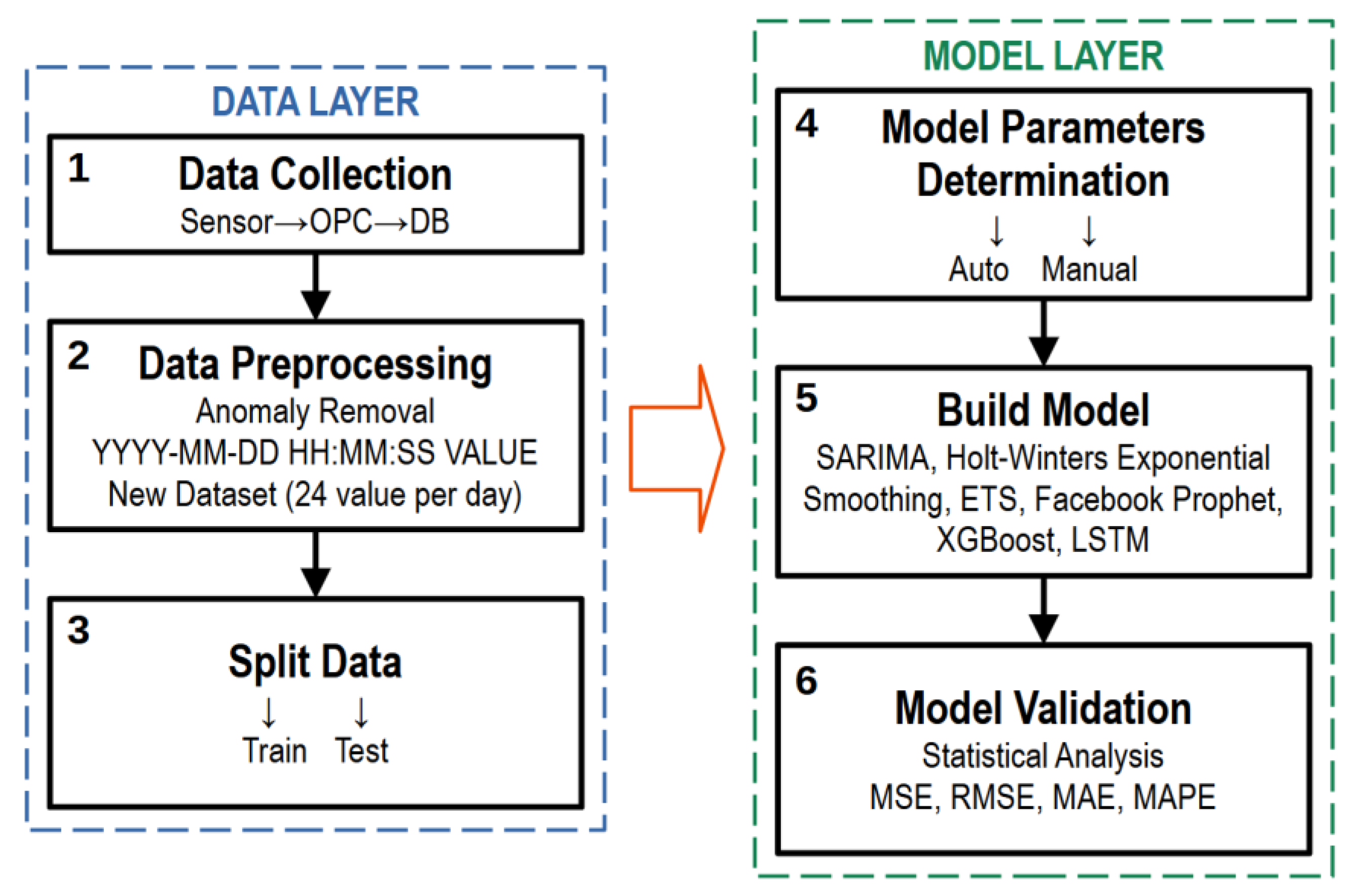
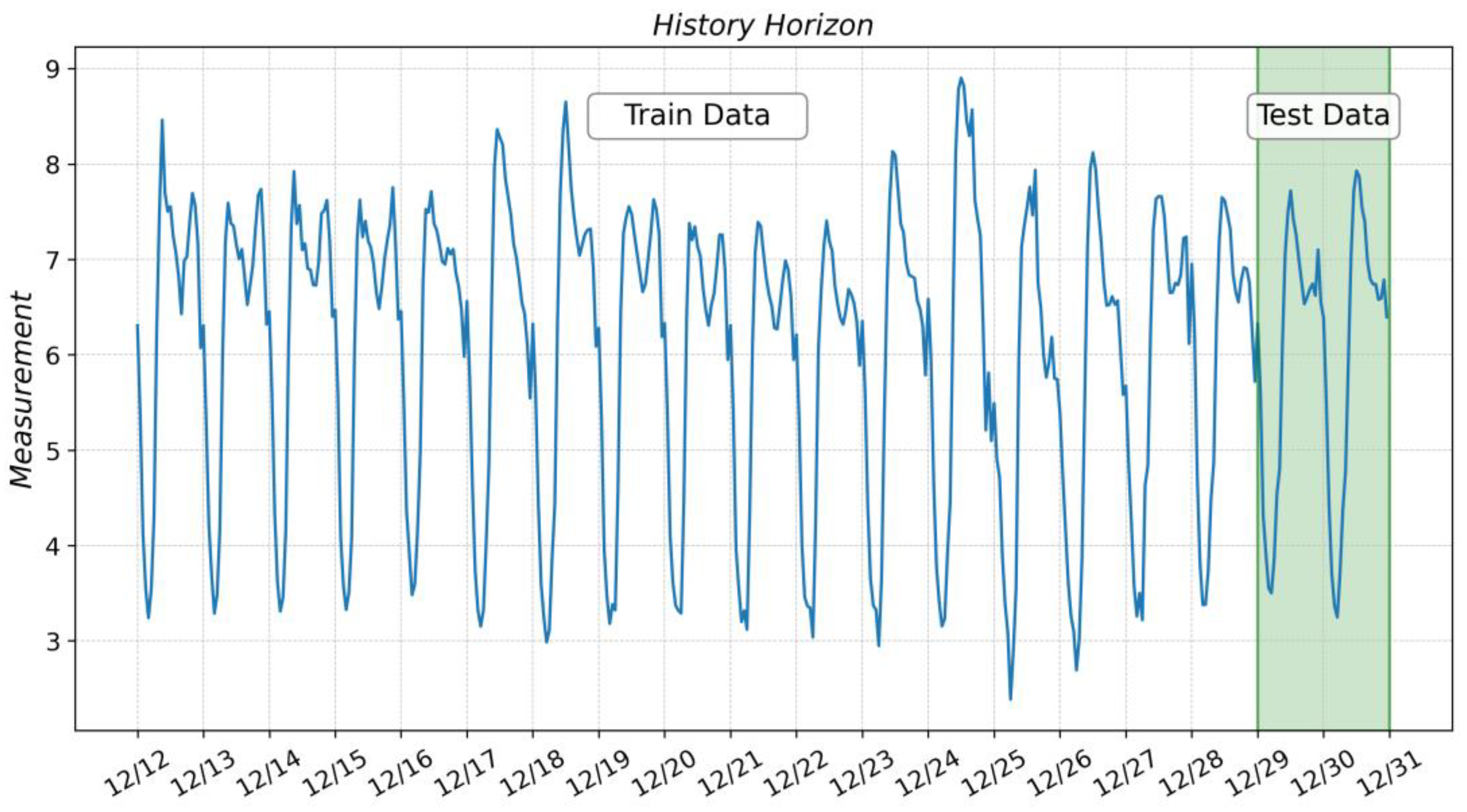
2.1. The Technical Roadmap and Data Collection

In this research, we used the actual data obtained from the monitoring system of the wastewater treatment plant. The monitoring system sensors collect basic parameters, such as input and output flow value, oxygen concentration, ammonia content, etc. Data from sensors come to the OPC server, and the OPC monitor records data with a frequency of once per second in synchronous and asynchronous modes. After the preprocessing, the monitoring system saves data in the database. The monitoring system operates 24/7, allowing obtaining data for any period of interest in the form of a comma-separated values format.
The model development process can generally be presented as a technical roadmap, shown in Figure 1.
There are two layers: the data layer and the model layer. Each layer is conventionally divided into three steps.
As described above, the data layer (steps 1–3) implements preprocessing and data preparation.
The model layer involves selecting model parameters (step 4), which can be implemented in two ways: automatically and manually. The selection method depends on the library’s capabilities to build the model. The next step (step 5) is model building, which involves setting the parameters defined in the previous step and training the model. At this step, all actions with the model can be called «model building». The last step (step 6) is the validation of the model. By «model validation», we mean obtaining a prediction and comparing the parameter estimates with their actual values. To assess the quality of the model, we will use a set of metrics described below. If the model metrics meet the specified ones, the model is saved and can be used to generate a forecast. If the metrics are unsatisfactory, you should return to step 4 and perform all subsequent steps at the data layer.
The estimation of the model’s accuracy was calculated with five statistical metrics: correlation coefficient (R2), mean squared error (MSE), root mean squared error (RMSE), mean absolute error (MAE), and mean absolute percentage error (MAPE) [12,37]. The correlation coefficient (R2) is used to determine the degree of fit of the forecasted values to the actual values. MSE is the average change in actual and forecast values, RMSE is the square root of MSE, and MAE is proposed as the average change between actual and predicted values. Compared with MAE, RMSE emphasizes the variance between data outliers. These metrics are calculated with equations:
R 2 = 1 i = 1 m y ^ i y i 2 i = 1 m 1 m i = 1 m y i y i 2 M S E = 1 m i = 1 m y ^ i y i 2 R M S E = 1 m i = 1 m y ^ i y i 2 M A E = 1 m i = 1 m y ^ i y i M A P E = 100 % 1 m i = 1 m y ^ i y i y i
where y i and y ^ i are the actual and predicted values, and m represents the number of samples.

2.2. Data Preprocessing

The data from the monitoring system sensors are stored in the database in raw form. This means that a simple upload of a parameter of interest over a specific time interval cannot be used as an input data set for model training. Pre-processing and filtering are required. The data format to be used in the vast majority of methods can be represented in general terms as D D M M Y Y Y Y   H H : M M : S S   V A L U E , where Y Y Y Y is a four-digit year code, M M is a two-digit current month code, D D is a two-digit day code, H H is a two-digit hour code, M M is a two-digit minute code, S S is a two-digit seconds code, and V A L U E is the real number corresponding to the parameter value obtained from the sensor.
As was mentioned above, the parameters are recorded with a frequency of 1 time per second. Since the resources of the monitoring system are limited, data averaged over 1 min are recorded in the database for each observed parameter. This frequency is also redundant for building an input flow prediction model, so the raw data obtained from the database underwent preprocessing. First, the data containing obvious outliers and anomalous values were discarded. At the next processing stage, the data were averaged over 1 h (resampling). As a result, a sample of data was generated for 19 days of observations, in which each day was represented by a set of 24 values of the observed parameter. The data set corresponding to the first 17 days of observations was used as training data. The remaining data were used to test the quality of the models. All preprocessing was performed using Pandas (Python Data Analysis Library) [38].
Table 1 shows a data slice of the entire dataset (total of 457 rows) obtained after applying the preprocessing procedure.
Figure 2 shows the periodicity of the process, with a seasoning period of 24 h. The data in the green area (Test Data) have been used to test the model quality, and the data to the left of the green area (Train Data) have been used to train the model. The task is formulated as follows: to build a predictive model using the available training dataset and use the model to build a forecast of the input stream for the next 48 h. Further steps are reduced to constructing and validating the obtained models using machine learning methods, discussed at the article’s beginning.
The following section will outline the main theoretical provisions and peculiarities of implementing the above methods using Python and open-source libraries.

3. Development of the Models
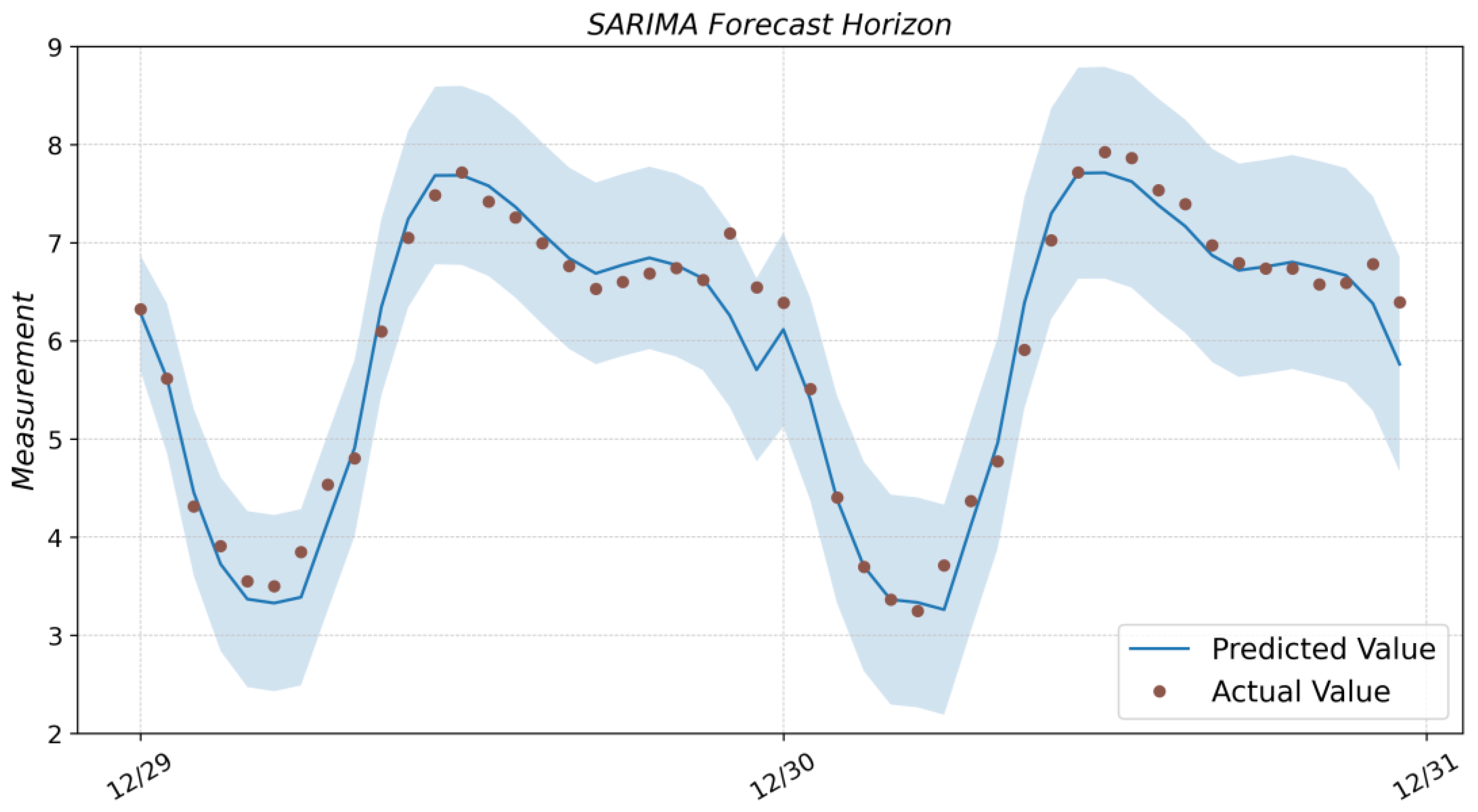
3.1. SARIMA

Seasonal Autoregressive Integrated Moving Average (SARIMA), or Seasonal ARIMA, is an extension of ARIMA that explicitly supports univariate time series data with a seasonal component. According to [39], the seasonal ARIMA model includes autoregressive and moving average terms at lag s .
The seasonal A R I M A p , d , q P , D , Q s model can be most succinctly expressed using the backward shift operator.
Θ P B s θ p B 1 B s D 1 B d x i = Φ Q B s ϕ q B ω t .
In Equation (2), Θ P ,   θ p ,   Φ Q and ϕ q are polynomials of orders P ,   p ,   Q and q , respectively. In general, the model is non-stationary, although, if D = d = 0 and the roots of the characteristic equation (polynomial terms on the left-hand side of Equation (1)) all exceed unity in absolute value, the resulting model would be stationary.
Thus, it is necessary to check the original dataset for stationarity before using the method. This can be performed using the Augmented Dickey-Fuller (ADfuller) test. This test is based on a hypothesis, where, if the p-value is less than 0.05, then we can consider the time series stationary, and if the p-value is greater than 0.05, then the time series is non-stationary.
To perform the ADfuller test and implement the SARIMA method, the library statmodels is used [40]. ADfuller test result are as follows:
Augmented Dickey-Fuller Test for SARIMA method
1. ADF : −6.162488723252326
2. P-Value : 7.118446442706881e−08
3. Num Of Lags : 18
4. Num Of Observations Used For ADF: 389
5. Critical Values :
   1% : −3.447272819026727
   5% : −2.868998737588248
   10% : −2.5707433189709294
Thus, the original time series is stationary.
The selection of parameters p , d , q P , D , Q can be performed automatically using the auto_arima function of the pmdarima library [41]. The result of the function is:
AutoARIMA. Performing stepwise search to minimize aic
ARIMA(2,0,1)(0,1,2)[24] intercept : AIC=191.369, Time=44.95 sec
ARIMA(1,0,2)(0,1,2)[24] intercept : AIC=184.365, Time=28.39 sec
ARIMA(1,0,2)(0,1,1)[24] intercept : AIC=202.174, Time=3.42 sec
ARIMA(1,0,2)(1,1,2)[24] intercept : AIC=inf, Time=31.94 sec
ARIMA(1,0,2)(1,1,1)[24] intercept : AIC=inf, Time=5.80 sec
ARIMA(0,0,2)(0,1,2)[24] intercept : AIC=218.241, Time=13.98 sec
ARIMA(2,0,2)(0,1,2)[24] intercept : AIC=177.020, Time=39.47 sec
ARIMA(2,0,2)(0,1,1)[24] intercept : AIC=194.216, Time=5.32 sec
ARIMA(2,0,2)(1,1,2)[24] intercept : AIC=inf, Time=51.64 sec
ARIMA(2,0,2)(1,1,1)[24] intercept : AIC=inf, Time=9.51 sec
ARIMA(3,0,2)(0,1,2)[24] intercept : AIC=176.735, Time=46.17 sec
ARIMA(3,0,2)(0,1,1)[24] intercept : AIC=191.289, Time=8.32 sec
ARIMA(3,0,2)(1,1,2)[24] intercept : AIC=inf, Time=54.78 sec
ARIMA(3,0,2)(1,1,1)[24] intercept : AIC=inf, Time=9.91 sec
ARIMA(3,0,1)(0,1,2)[24] intercept : AIC=177.137, Time=37.80 sec
ARIMA(3,0,3)(0,1,2)[24] intercept : AIC=181.003, Time=48.34 sec
ARIMA(2,0,3)(0,1,2)[24] intercept : AIC=177.237, Time=51.24 sec
ARIMA(3,0,2)(0,1,2)[24]       : AIC=169.441, Time=44.18 sec
ARIMA(3,0,2)(0,1,1)[24]       : AIC=185.525, Time=9.49 sec
ARIMA(3,0,2)(1,1,2)[24]       : AIC=inf, Time=52.88 sec
ARIMA(3,0,2)(1,1,1)[24]       : AIC=inf, Time=9.48 sec
ARIMA(2,0,2)(0,1,2)[24]       : AIC=178.763, Time=26.75 sec
ARIMA(3,0,1)(0,1,2)[24]       : AIC=178.903, Time=25.43 sec
ARIMA(3,0,3)(0,1,2)[24]       : AIC=182.748, Time=31.08 sec
ARIMA(2,0,1)(0,1,2)[24]       : AIC=177.159, Time=28.53 sec
ARIMA(2,0,3)(0,1,2)[24]       : AIC=178.965, Time=39.95 sec
Best model: ARIMA(3,0,2)(0,1,2)[24]
Total fit time: 865.904 seconds
Where s = 24 is the period of the seasonal time series in hours.
After the model is built considering the obtained optimal parameters, in order to make a prediction, it is sufficient to use the get_forecast method of the model object, passing as a parameter the number of time counts, for which we need to obtain a prediction. Since the interval between the samples in the initial dataset is 1 h, and the forecast is made for 48 h, you should specify the input parameter steps = 48.
Figure A1 (see Appendix A) shows the time series plot obtained with the SARIMA model (solid blue line on the plot) and the actual measurement values from the test data set (dark bullet marker on the plot). The Section 4 will give a quantitative assessment of the quality of this and subsequent predictive models.

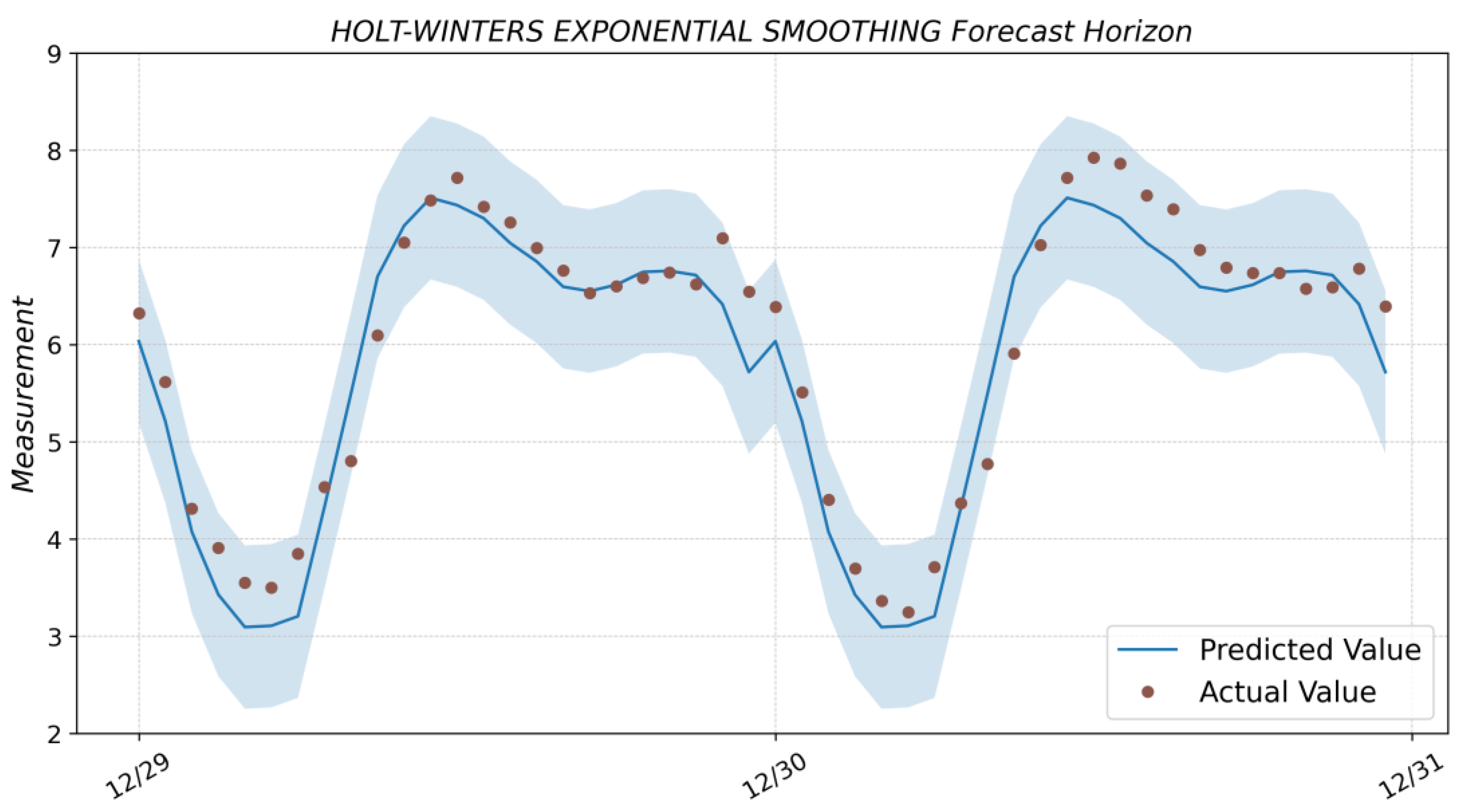
3.2. Holt-Winters Exponential Smoothing
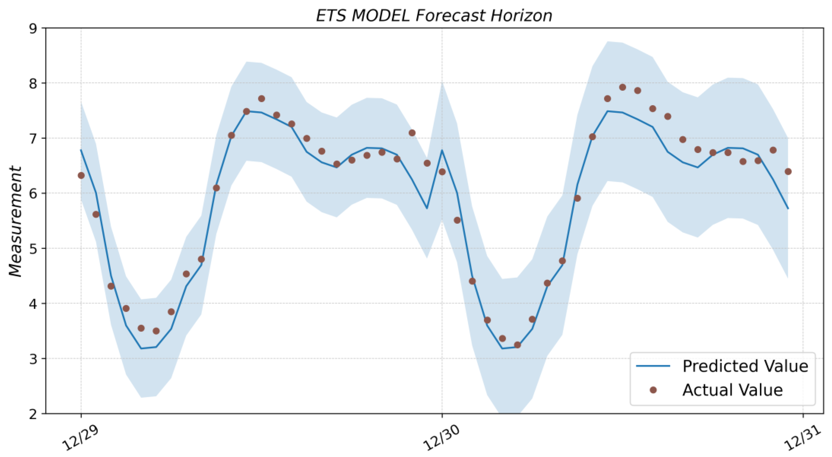
The Holt-Winters seasonal method comprises the forecast equation and three smoothing equations—one for the level t , one for the trend b t , and one for the seasonal component s t , with corresponding smoothing parameters α ,   β * and γ .
The parameter m is used to denote the seasonality period [42]. Two variations of this method differ from the seasonal component—the additive and multiplicative methods.
The component form for the additive method is:
y ^ t + h | t = t + h b t + s t + h m k + 1 t = α y t s t m + 1 α t 1 + b t 1 b t = β * t t 1 + 1 β * b t 1 s t = γ y t t 1 b t 1 + 1 γ s t m   .
The component form for the multiplicative method is:
y ^ t + h | t = t + h b t + s t + h m k + 1 t = α y t s t m + 1 α t 1 + b t 1 b t = β * t t 1 + 1 β * b t 1 s t = γ y t t 1 b t 1 + 1 γ s t m   .
The k in Equations (3) and (4) is the integer part of h 1 / m . The level equation t shows a weighted average between the seasonally adjusted observation y t s t m and the non-seasonal forecast t t 1 for time t . The trend equation b t is identical to Holt’s linear method. The seasonal equation shows a weighted average between the current seasonal index, y t t 1 b t 1 , and the seasonal index of the same season m time periods ago. The s t is an equation for the seasonal component. To create a predictive model based on the Holt-Winters Exponential Smoothing method, the function Exponential Smoothing of the statmodels library [40] is used. The function takes three parameters as input: the data set for training, the type of seasonal component add/mul, and the value of the parameter m from Equations (2) and (3)—the value of the seasonality period of the sample. The result of forecasting with the Holt-Winters model is shown in Figure A2 (see Appendix A).

3.3. ETS

The ETS models are a family of time series models with an underlying state space model consisting of a level component, a trend component (T), a seasonal component (S), and an error term (E). Point forecasts can be obtained from the models by iterating the equations for t = T + 1 ,   ,   T + h and setting all = 0 for t > T . For example, for the model, ETS (M, A, N) = 1 + ε T + 1 . Therefore y ^ T + 1 | T = T + b T . Similarly,
y T + 2 = T + 1 + b T + 1 1 + ε T + 2 = T + b T 1 + α ε T + 1 + b T + β T + b T ε T + 1 1 + ε T + 2 .  
Therefore, y ^ T + 2 | T = T + 2 b T , and so on (see Equation (5)). These forecasts are identical to the forecasts from Holt’s linear method and also to those from model ETS (A, A, N). Thus, the point forecasts obtained from the method and from the two models that underlie the method are identical (assuming that the same parameter values are used). The ETS point forecasts constructed in this way are equal to the means of the forecast distributions, except for the models with multiplicative seasonality [42]. As with the Holt-Winters model, the ETS model can be obtained using the statmodels library. The ETSModel function takes as input parameters an array of data with time series counts, a flag defining seasonal component type add/mul, and seasonal period value (for the example under consideration seasonal_periods = 24). The get_prediction method of the model object, which receives as input parameters two timestamp values corresponding to the start and end time for the desired prediction horizon, is used to obtain the prediction. When using pandas, these values can be found as start and end values of the pandas dataframe object index, where the test selection of the time series is stored. The result for the ETS model is shown in Figure A3 (see Appendix A).

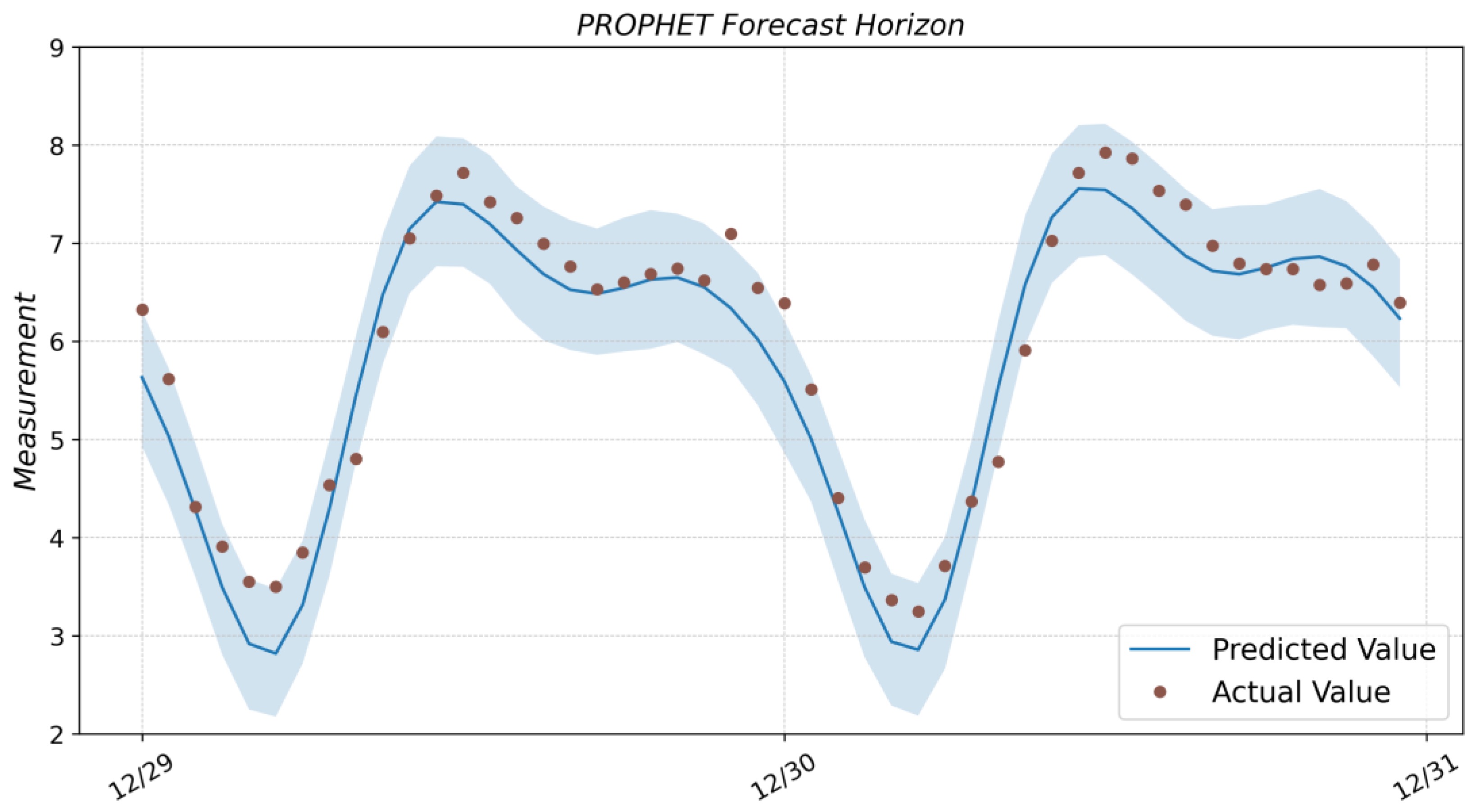
3.4. Facebook Prophet
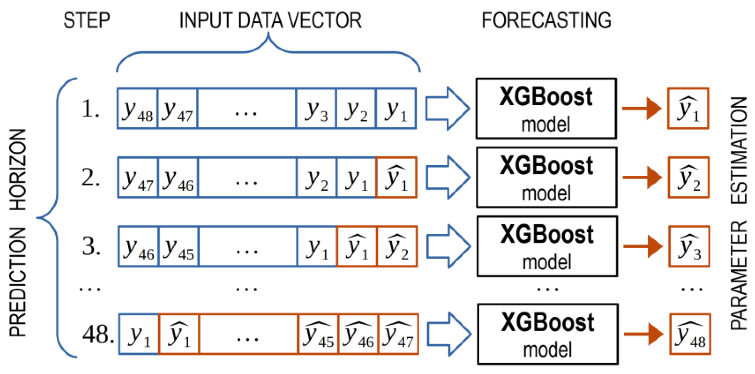
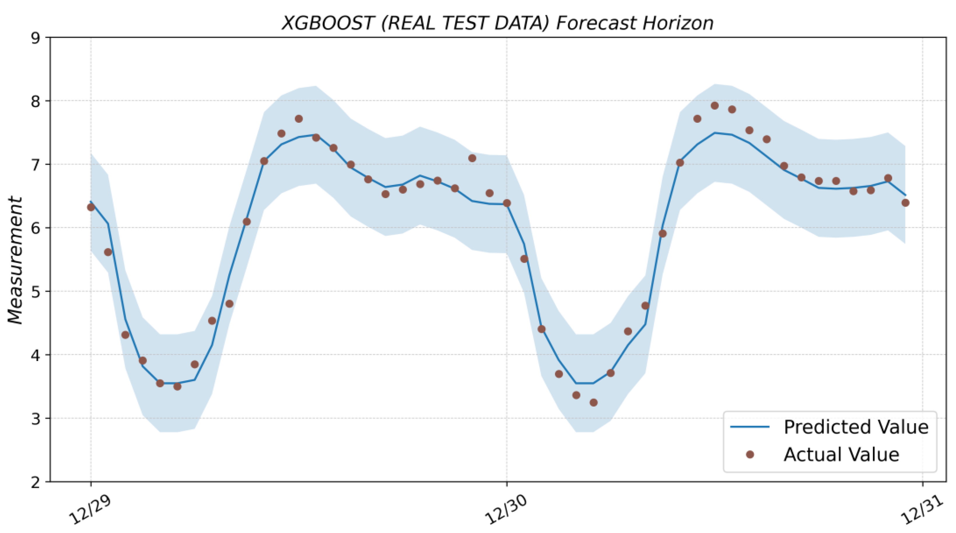
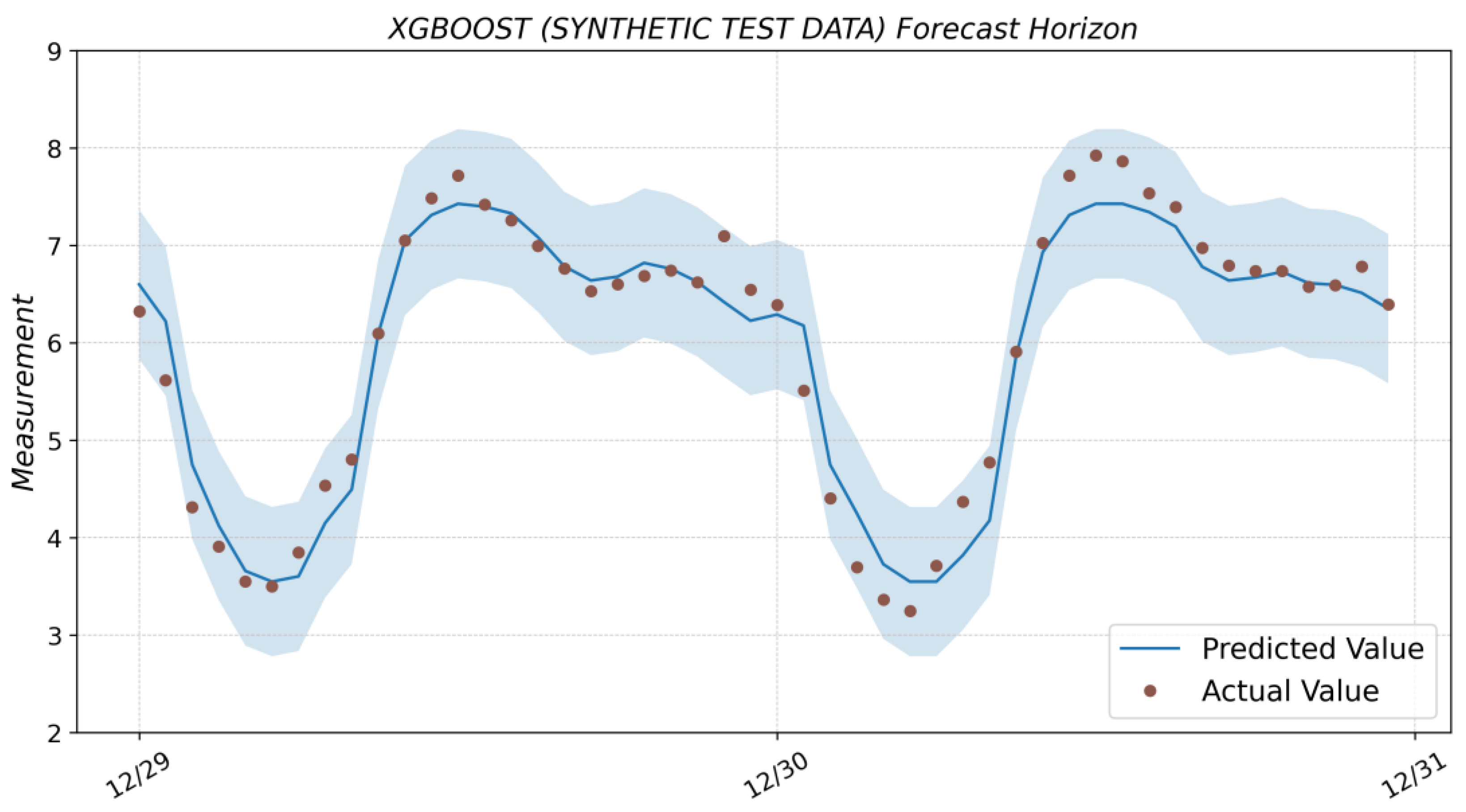
Prophet is a procedure for forecasting time series data based on an additive regression model, where non-linear trends are fit with yearly, weekly, and daily seasonality, plus holiday effects. It works best with time series that have strong seasonal effects and several seasons of historical data. Prophet is robust to missing data and shifts in the trend, and it typically handles outliers well [43]. The main idea of the method is presented in [31]. The Prophet is an open-source library that is distributed in R and Python. The selection of the required model parameters is fully automated, so to build a model, it is sufficient to pass the input dataset for training. The Prophet function of the prophet library is used to create the model. Predicted parameter values can be found using the prediction model method, with a data frame of time stamps corresponding to the prediction horizon as input. The result of forecasting with the Prophet model is shown in Figure A4 (see Appendix A).

3.5. XGBoost

Extreme Gradient Boosting (XGBoost) is an optimized distributed gradient boosting library designed to be highly efficient, flexible, and portable. It implements machine learning algorithms under the Gradient Boosting framework. XGBoost provides a parallel tree boosting (also known as GBDT, GBM) that solves many data science problems in a fast and accurate way. The same code runs on the major distributed environment (Hadoop, SGE, MPI) and can solve problems beyond billions of examples [44].
The main idea of the method is presented in [32]. The model is created using the XGBRegressor function of the xgboost library. The function contains a relatively large number of parameters, and a complete list can be found in the documentation section of the library [45]. In our case, only four parameters were used:
  • max_depth = 6—maximum tree depth for base learners;
  • learning_rate = 0.05—boosting learning rate (xgb’s “eta”);
  • n_estimators = 5000—number of gradients boosted trees (equivalent to the number of boosting rounds);
  • gamma = 0.1—minimum loss reduction required to make a further partition on a leaf node of the tree.
It should be noted that, in contrast to the previously described implementations, the xgboost library can predict only one step ahead. Previous methods allowed setting the forecast horizon length in hours after training the model, after which the model output produced an estimate of the observed parameter. The XGBoost model allows one to obtain a forecast only for one step ahead (i.e., for 1 h). The aim is to obtain the forecast 48 h ahead. It is necessary to change the scheme of data preparation, which is fed to the model input. The algorithm for generating the data used to train and test the model is as follows:
  • To generate a forecast for 1 h ahead, the model’s input is the historical sample for the previous 48 h. The model’s output estimates the observed parameter 1 h ahead.
  • One element shifts the historical sample dataset to the left, and as a result, its length is reduced by 1. An element is placed in the place of the missing element at the end of the sample—the estimate of the observed parameter obtained at the previous step. A new parameter estimate is obtained at the model’s output, corresponding to the 2-h forecast horizon.
  • Iterations continue until the desired forecast horizon is obtained.
An explanation of this algorithm for the task of obtaining a forecast horizon for the next 48 h is shown in Figure 3. A similar approach was used to prepare data for the Long Short-Term Memory model.
When testing the model, you can use actual data from the test dataset instead of parameter estimates (real test data), but to obtain a prediction in a real-time system, you will have to use parameter estimates to generate a new dataset (synthetic test data). Below, the results will be given for real and synthetic test data.
The result of forecasting with the XGBoost model based on real and synthetic test data is shown in Figure A5 and Figure A6 (see Appendix A).
As follows from the graphical results, we can conclude that, when using synthetic test data (i.e., the system works in real conditions), the accuracy will decrease as the forecast horizon increases. That is why we should either increase the amount of data in the input vector fed into the model or decrease the forecast horizon. The accuracy of the model will also be affected by the XGBoost model setup.

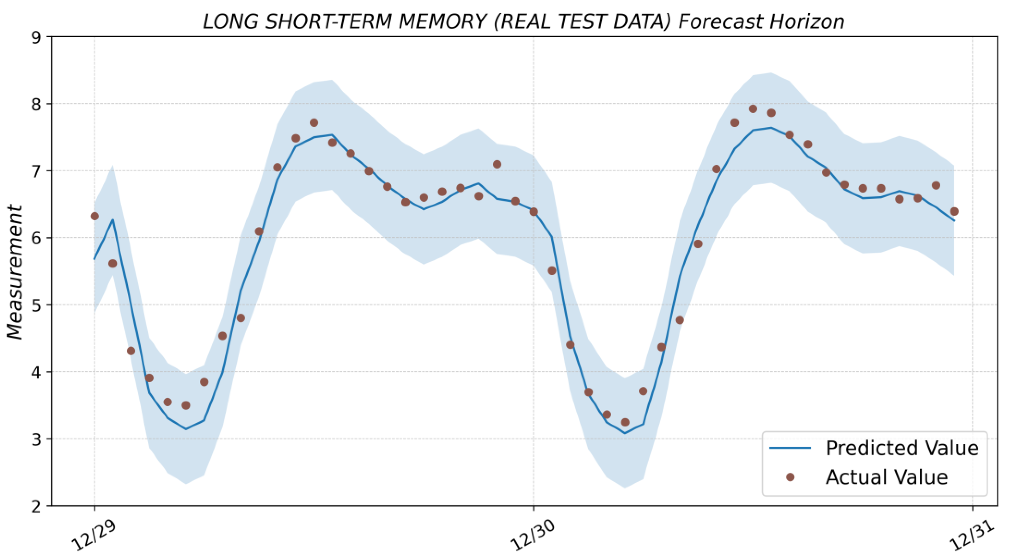
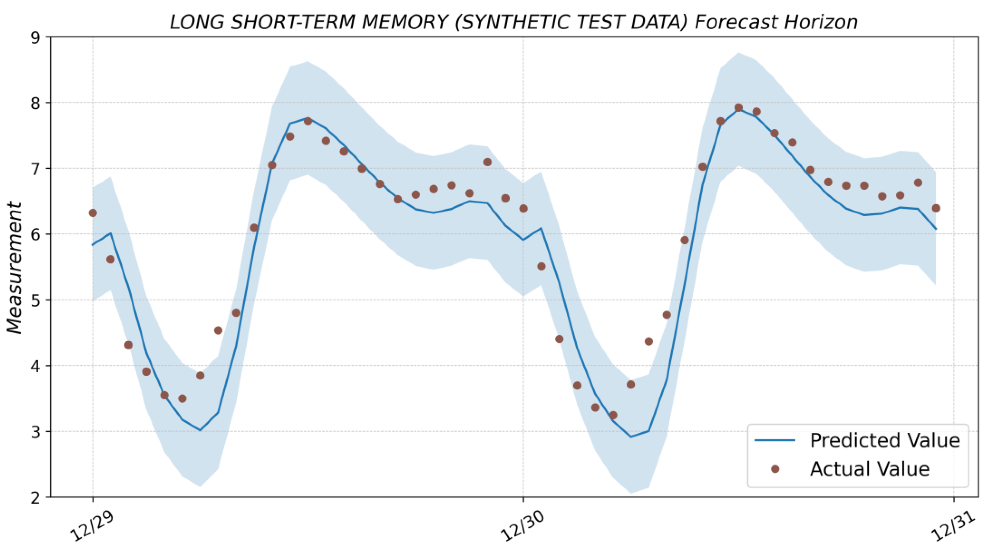
3.6. Long Short-Term Memory

Long Short-Term Memory (LSTM) is an artificial neural network in artificial intelligence and deep learning. Unlike standard feedforward neural networks, LSTM has feedback connections. Such a recurrent neural network (RNN) can process single data points and entire data sequences. This characteristic makes LSTM networks ideal for processing and predicting data, including time series. The main idea of the method is presented in [21].
To build the LSTM model, we used the keras library and a set of functions Sequential, Dense, and LSTM, which were used to set the structure of the neural network. The following parameters were chosen to build the model:
  • batch_size = 16—number of samples per gradient update;
  • epochs = 200—number of epochs to train the model;
  • units = 32—dimensionality of the output space.
A description of the LTSM model obtained using the keras library is shown below.
Algorithms 16 00248 i001
The result of forecasting with the LSTM model based on real and synthetic test data is shown in Figure A7 and Figure A8 (see Appendix A).

4. Results and Discussion

Table 2 shows the results of calculating statistical metrics to assess the accuracy of the created models. The first columns are the statistical metrics, T.Time is the time in seconds that it took to build the model, and P.Time is the time in seconds to calculate the prediction. The build model time includes the time to obtain all necessary data, optimal parameter selection, and model time creation with the Python libs.
All models show good quality with a good R-squared metric > 0.9. The models with R-squared > 0.95 shows excellent accuracy. However, the second factor—time for preprocessing and training models and time to obtain the forecasting—will be used to choose the best model.
The leaders in accuracy are three models: SARIMA, LSTM, and XGBoost. However, SARIMA and LSTM significantly lose the time required to create a new model, which is caused by the automatic procedure of selecting parameters. The SARIMA method has high accuracy, but its application in systems with non-stationary time series with seasonal variability can be complex because of the long time required for automatic model preparation. The LSTM method showed promising results on accurate data. Still, the accuracy decreases significantly on synthetic test data, i.e., the forecast horizon for natural systems will decrease to preserve the precision. This indicates that the method has good potential but requires more careful tuning, network structure choice, and input data optimization for training and model use. XGBoost requires less than 10 s for fully automatic model building. The time it takes to obtain a prediction when the control signal is applied once per second is 0.2 s, i.e., about 20%. In addition to Python, the XGBoost libraries are implemented in the C++/C# programming languages, making it easy to bring it into production. Therefore, the optimal choice for solving the task is the XGBoost method.
It should be noted that this study has limitations: we assume that the sensors are working correctly. New data are always coming in. If the system is interrupted for more than two days, it will be necessary to accumulate new continuous historical data for the last two to three weeks before starting.

5. Conclusions

The article considers various methods of forecasting time series with seasonality. Classical and newer approaches based on machine learning algorithms and neural networks, as well as statistical models, are presented. A test of prediction accuracy using statistical metrics was performed for each of the considered methods. The authors proposed an approach that allows using small historical data samples (less than 21 days) to build a short-term forecast (nearest 48 h). It reduces the load on computing resources and maintains the accuracy of the estimates. It is crucial when implementing predictive systems based on embedded devices that implement real-time automatic control. The model must be retrained once a day to achieve the goal, considering the newly received data. Thus, the criterion responsible for the time for collecting data, training the model, and obtaining a forecast plays a decisive role in choosing a model. The best method, according to a set of attributes, turned out to be the XGBoost method. Nevertheless, optimizing algorithms to search model parameters can bring other algorithms, such as LSTM, to the forefront. Further research will be devoted to the optimization of model learning. A new approach for the hyperparameters finding procedure and a new algorithm for the optimal data length calculation should be developed. The existing methods will be extended for the using of the recommended systems and robust optimal control real-time systems. The participation of the operator in setting up the algorithms should be minimized.

Author Contributions

Conceptualization, V.K. and V.A.; methodology, V.K.; software, V.A.; formal analysis, V.K.; investigation, V.K. and V.A.; writing—original draft preparation, V.A.; writing—review and editing, V.K.; visualization, V.A.; supervision, V.K.; All authors have read and agreed to the published version of the manuscript.

Funding

This research received no external funding.

Institutional Review Board Statement

Not applicable.

Informed Consent Statement

Not applicable.

Data Availability Statement

The code and data presented in this study available on GitHub “https://github.com/vasoftlab/algorithms-16-00248 (accessed on 8 May 2023)”. All details can be provided upon request from the corresponding author.

Conflicts of Interest

The authors declare no conflict of interest.

Abbreviations

The following abbreviations are used in this manuscript:
ADfullerAugmented Dickey-Fuller
ANNArtificial Neural Network
ARIMAAutoregressive integrated moving average
DBData base
ETSExponential smoothing
LSTMLong short-term memory
MAEMean absolute error
MAPEMean absolute percentage error
MSEMean squared error
OPCOpen Platform Communications
P.TimePrediction time
R2Correlation coefficient
RMSERoot mean squared error
RNNRecurrent neural network
SARIMASeasonal autoregressive integrated moving average
T.TimeTraining time

Appendix A

Figure A1. Prediction result with SARIMA model and actual values from the test dataset.
Algorithms 16 00248 g0a1
Figure A2. Prediction result with Holt-Winters Exponential Smoothing model and actual values from the test dataset.
Algorithms 16 00248 g0a2
Figure A3. Prediction result with ETS model and actual values from the test dataset.
Algorithms 16 00248 g0a3
Figure A4. Prediction result with Prophet model and actual values from the test dataset.
Algorithms 16 00248 g0a4
Figure A5. Prediction result with the XGBoost model (based on real test data) and actual values from the test dataset.
Algorithms 16 00248 g0a5
Figure A6. Prediction result with the XGBoost model (based on synthetic test data) and actual values from the test dataset.
Algorithms 16 00248 g0a6
Figure A7. Prediction result with the LSTM model (based on real test data) and actual values from the test dataset.
Algorithms 16 00248 g0a7
Figure A8. Prediction result with the LSTM model (based on synthetic test data) and actual values from the test dataset.
Algorithms 16 00248 g0a8

Appendix B

Algorithm A1: XGBoost model retraining and prediction (48 h ahead)
1 t i m e s t a r t ;   t i m e s t o p The time interval for the training data
2 d a t a _ p r e p r o c e s s i n g t i m e s t a r t ,   t i m e s t o p Resample and training data generation
3 Output :   X _ t r a i n ,   y _ t r a i n
4 m a x d e p t h =  6Maximum tree depth for base learners
5 l e a r n i n g r a t e =  0.05Boosting learning rate
6 n e s t i m a t o r s =  5000Number of gradients boosted trees
7 g a m m a =  0.1Minimum loss reduction
8 m o d e l = X G B R e g r e s s o r ( o b j e c t i v e = r e g : s q u a r e d e r r o r , XGBoost regressor
9 n _ e s t i m a t o r s = n _ e s t i m a t o r s ,
10 m a x _ d e p t h = m a x _ d e p t h ,
11 l e a r n i n g _ r a t e = l e a r n i n g _ r a t e ,
12 g a m m a = g a m m a )
13 m o d e l . f i t X _ t r a i n ,   y _ t r a i n Training model
14 y _ p r e d _ n e w = [ ] Prediction array initialization
15 for   i = 1   t o   48   d o
9 x _ l i s t = x _ t r a i n . i l o c : ,   1 : . v a l u e s . t o l i s t ( )
10 y _ l i s t = y _ p r e d . t o l i s t ( )
11 x _ t r a i n = p d . D a t a F r a m e x _ l i s t 0 + y _ l i s t 0 New train data
12 x _ t r a i n = x _ t r a i n . t r a n s p o s e ( )
13 y _ p r e d = m o d e l . p r e d i c t x _ t r a i n Get prediction
14 y _ p r e d = p d . D a t a F r a m e y _ p r e d Convert to the Pandas dataframe
15 y _ p r e d = y _ p r e d . v a l u e s
16 y _ p r e d _ n e w . a p p e n d ( y _ p r e d . t o l i s t ( ) 0 ) Add new predicted value
17 end   for
18 Output :   y _ p r e d _ n e w Prediction dataset for the next 48 hrs

References

  1. Nguyen, G.; Dlugolinsky, S.; Bobák, M. Machine learning and deep learning frameworks and libraries for large-scale data mining: A survey. Artif. Intell. Rev. 2019, 52, 77–124. [Google Scholar] [CrossRef]
  2. Makridakis, S.; Wheelwright, S.C.; Hyndman, R.J. Forecasting Methods and Applications; John Wiley and Sons: Hoboken, NJ, USA, 2008. [Google Scholar]
  3. Box, G.E.P.; Jenkins, G.M. Time Series Analysis: Forecasting and Control; John Wiley and Sons: Hoboken, NJ, USA, 2008. [Google Scholar]
  4. Martínez-Álvarez, F.; Troncoso, A.; Asencio-Cortés, G.; Riquelme, J.C. A survey on data mining techniques applied to electricity-related time series forecasting. Energies 2015, 8, 13162–13193. [Google Scholar] [CrossRef]
  5. Fu, T.C. A review on time series data mining. Eng. Appl. Artif. Intell. 2011, 24, 164–181. [Google Scholar] [CrossRef]
  6. Torres, J.F.; Galicia, A.; Troncoso, A. A scalable approach based on deep learning for big data time series forecasting. Integr. Comput.-Aided Eng. 2018, 25, 335–348. [Google Scholar] [CrossRef]
  7. Liu, Z.; Jiang, P.; Zhang, L.; Niu, X. A combined forecasting model for time series: Application to short-term wind speed forecasting. Appl. Energy 2020, 259, 114137. [Google Scholar] [CrossRef]
  8. Torres, J.; Hadjout, D.; Sebaa, A.; Martínez-Álvarez, F.; Troncoso, A. Deep Learning for Time Series Forecasting: A Survey. Big Data 2020, 9, 3–21. [Google Scholar] [CrossRef]
  9. Hajirahimi, Z.; Khashei, M. Hybrid structures in time series modeling and forecasting: A review. Eng. Appl. Artif. Intell. 2019, 86, 83–106. [Google Scholar] [CrossRef]
  10. Gasparin, A.; Lukovic, S.; Alippi, C. Deep learning for time series forecasting: The electric load case. CAAI Trans. Intell. Technol. 2021, 7, 1–25. [Google Scholar] [CrossRef]
  11. Pongdatu, G.A.N.; Putra, Y.H. Time Series Forecasting using SARIMA and Holt Winter’s Exponential Smoothing. IOP Conf. Ser. Mater. Sci. Eng. 2018, 407, 012153. [Google Scholar] [CrossRef]
  12. Huang, W.; Li, Y.; Zhao, Y.; Zheng, L. Time Series Analysis and Prediction on Bitcoin. BCP Bus. Manag. 2022, 34, 1223–1234. [Google Scholar] [CrossRef]
  13. Kemalbay, G.; Korkmazoglu, O.B. Sarima-arch versus genetic programming in stock price prediction. Sigma J. Eng. Nat. Sci. 2021, 39, 110–122. [Google Scholar] [CrossRef]
  14. Paliari, I.; Karanikola, A.; Kotsiantis, S. A comparison of the optimized LSTM, XGBOOST and ARIMA in Time Series forecasting. In Proceedings of the 12th International Conference on Information, Intelligence, Systems & Applications (IISA), Chania Crete, Greece, 12–14 July 2021. [Google Scholar]
  15. Andreeski, C.; Mechkaroska, D. Modelling, Forecasting and Testing Decisions for Seasonal Time Series in Tourism. Acta Polytech. Hung. 2020, 17, 149–171. [Google Scholar] [CrossRef]
  16. Uğuz, S.; Büyükgökoğlan, E. A Hybrid CNN-LSTM Model for Traffic Accident Frequency Forecasting during the Tourist Season. Teh. Vjesn.–Tech. Gaz. 2022, 29, 2083–2089. [Google Scholar]
  17. Etuk, E. A seasonal time series model for Nigerian monthly air traffic data. IJRRAS 2013, 14, 596–602. [Google Scholar]
  18. Feng, T.; Tianyu, Z.; Zheng, Y.; Jianxing, Y. The comparative analysis of SARIMA, Facebook Prophet, and LSTM for road traffic injury prediction in Northeast China. Front. Public Health 2022, 10, 946563. [Google Scholar] [CrossRef]
  19. Zhu, X.; Helmer, E.H.; Gwenzi, D.; Collin, M. Characterization of Dry-Season Phenology in Tropical Forests by Reconstructing Cloud-Free Landsat Time Series. Remote Sens. 2021, 13, 4736. [Google Scholar] [CrossRef]
  20. Figueiredo, N.; Blanco, C. Water level forecasting and navigability conditions of the Tapajós River–Amazon–Brazil. La Houille Blanche 2016, 3, 53–64. [Google Scholar] [CrossRef]
  21. Shen, J.; Valagolam, D.; McCalla, S. Prophet forecasting model: A machine learning approach to predict the concentration of air pollutants (PM2.5, PM10, O3, NO2, SO2, CO) in Seoul, South Korea. PeerJ 2020, 8, e9961. [Google Scholar] [CrossRef]
  22. Hasnain, A.; Sheng, Y.; Hashmi, M.Z. Time Series Analysis and Forecasting of Air Pollutants Based on Prophet Forecasting Model in Jiangsu Province, China Citation. Front. Environ. Sci. 2022, 10, 1044. [Google Scholar] [CrossRef]
  23. Luo, Z.; Jia, X.; Bao, J. A Combined Model of SARIMA and Prophet Models in Forecasting AIDS Incidence in Henan Province, China. Int. J. Environ. Res. Public Health 2022, 19, 5910. [Google Scholar] [CrossRef]
  24. Pandit, A.; Khan, D.Z.; Hanrahan, J.G. Historical and future trends in emergency pituitary referrals: A machine learning analysis. Pituitary 2022, 25, 927–937. [Google Scholar] [CrossRef] [PubMed]
  25. Benkachcha, S.; Benhra, J.; El Hassani, H. Seasonal Time Series Forecasting Models based on Artificial Neural Network. Int. J. Comput. Appl. 2015, 116, 9–14. [Google Scholar]
  26. Palmroos, C.; Gieseler, J.; Morosan, N. Solar energetic particle time series analysis with Python. Front. Astron. Space Sci. 2022, 9, 1073578. [Google Scholar] [CrossRef]
  27. Wan, X.; Zou, Y.; Wang, J.; Wang, W. Prediction of shale oil production based on Prophet algorithm. J. Phys. Conf. Ser. 2021, 2009, 012056. [Google Scholar] [CrossRef]
  28. El-Rawy, M.; Abd-Ellah, M.K.; Fathi, H.; Abdella Ahmed, A.K. Forecasting effluent and performance of wastewater treatment plant using different machine learning techniques. J. Water Process Eng. 2021, 44, 102380. [Google Scholar] [CrossRef]
  29. Ding, Z.; Yu, Y.; Xia, Y. Nonlinear hysteretic parameter identification using an attention-based long short-term memory network and principal component analysis. Nonlinear Dyn 2023, 111, 4559–4576. [Google Scholar] [CrossRef]
  30. Yu, Y.; Liang, S.; Samali, B.; Nguyen, T.N.; Zhai, C.; Li, J.; Xie, X. Torsional capacity evaluation of RC beams using an improved bird swarm algorithm optimized 2D convolutional neural network. Eng. Struct. 2022, 273, 115066. [Google Scholar] [CrossRef]
  31. Taylor, S.; Letham, B. Forecasting at scale. Am. Stat. 2018, 72, 37–45. [Google Scholar] [CrossRef]
  32. Chen, T.; Guestrin, C. XGBoost: A Scalable Tree Boosting System. In Proceedings of the 22nd ACM SIGKDD International Conference, San Francisco, CA, USA, 13 August 2016; pp. 785–794. [Google Scholar]
  33. Hochreiter, S.; Schmidhuber, J. Long Short-term Memory. Neural Comput. 1997, 9, 1735–1780. [Google Scholar] [CrossRef]
  34. Rumelhart, D.; Hinton, G.; Williams, R. Long short-term memory. Naturev 1986, 323, 533–536. [Google Scholar] [CrossRef]
  35. Anqi, X.; Hao, Y.; Jing, C.; Li, S.; Qian, Z. A Short-Term Wind Speed Forecasting Model Based on a Multi-Variable Long Short-Term Memory Network. Atmosphere 2021, 12, 651. [Google Scholar]
  36. Zemkoho, A. A Basic Time Series Forecasting Course with Python. Oper. Res. Forum 2023, 4, 2. [Google Scholar] [CrossRef]
  37. Plevris, V.; Solorzano, G.; Bakas, N.; Ben Seghier, M. Investigation of Performance Metrics in Regression Analysis and Machine Learning-Based Prediction Models. In 8th European Congress on Computational Methods in Applied Sciences and Engineering (ECCOMAS 2022) at Oslo; European Community on Computational Methods in Applied Sciences: Barcelona, Spain, 2022. [Google Scholar]
  38. Pandas—Python Data Analysis Library. Available online: https://pandas.pydata.org/ (accessed on 3 February 2023).
  39. Cowpertwait, P.S.P.; Metcalfe, A.V. Introductory Time Series with R; Springer: Berlin/Heidelberg, Germany, 2009; pp. 142–143. [Google Scholar]
  40. Introduction—Statmodels. Available online: https://www.statsmodels.org/stable/index.html/ (accessed on 3 February 2023).
  41. Pmdarima: ARIMA Estimators for Python. Available online: https://alkaline-ml.com/pmdarima/index.html (accessed on 3 February 2023).
  42. Hyndman, R.J.; Athanasopoulos, G. Forecasting: Principles and Practice, 3rd ed.; Otexts, Monash University: Melbourne, Australia, 2022. [Google Scholar]
  43. Prophet|Forecasting at Scale. Available online: https://facebook.github.io/prophet/ (accessed on 3 February 2023).
  44. XGBoost. Available online: https://xgboost.ai/about (accessed on 3 February 2023).
  45. Python API Reference—XGBoost Documentation. Available online: https://xgboost.readthedocs.io/en/stable/python/index.html (accessed on 3 February 2023).
Figure 1. The technical roadmap of data analysis.
Algorithms 16 00248 g001
Figure 2. Initial dataset with a breakdown into training and test samples.
Algorithms 16 00248 g002
Figure 3. Data preprocessing algorithm for the XGBoost model.
Algorithms 16 00248 g003
Table 1. The slice of the entire dataset.
IDTimestampMeasurement
012 December 2022 00:00:006.305967
112 December 2022 01:00:005.355895
212 December 2022 02:00:004.122726
312 December 2022 03:00:003.546737
45230 December 2022 20:00:006.578148
45330 December 2022 21:00:006.591513
45430 December 2022 22:00:006.785699
45530 December 2022 23:00:006.396174
45631 December 2022 00:00:006.322228
Table 2. Statistical and performance time analysis.
ModelR2MSERMSEMAEMAPET.TimeP.Time
SARIMA0.9610.0760.2760.1980.0351298.0600.020
Holt-Winters ES0.9210.1560.3960.3240.0590.0490.001
ETS0.9450.1090.3290.2540.0430.2850.001
Prophet0.9180.1620.4020.3310.0620.8810.754
XGBoost (real test data)0.9750.0500.2240.1630.0297.5050.005
XGBoost (synthetic test data)0.9540.0910.3010.2280.0437.5050.235
LSTM (real test data)0.9600.0800.2820.2180.04139.5050.361
LSTM (synthetic test data)0.9070.1840.4290.3220.06339.5053.185
Disclaimer/Publisher’s Note: The statements, opinions and data contained in all publications are solely those of the individual author(s) and contributor(s) and not of MDPI and/or the editor(s). MDPI and/or the editor(s) disclaim responsibility for any injury to people or property resulting from any ideas, methods, instructions or products referred to in the content.

