Article

Forgetful Forests: Data Structures for Machine Learning on Streaming Data under Concept Drift

Courant Institute of Mathematical Science, New York University, New York, NY 10012, USA
*
Author to whom correspondence should be addressed.
Algorithms 2023, 16(6), 278; https://doi.org/10.3390/a16060278
Submission received: 9 May 2023 / Revised: 25 May 2023 / Accepted: 26 May 2023 / Published: 31 May 2023
(This article belongs to the Special Issue Machine Learning for Time Series Analysis)

Abstract

:
Database and data structure research can improve machine learning performance in many ways. One way is to design better algorithms on data structures. This paper combines the use of incremental computation as well as sequential and probabilistic filtering to enable “forgetful” tree-based learning algorithms to cope with streaming data that suffers from concept drift. (Concept drift occurs when the functional mapping from input to classification changes over time). The forgetful algorithms described in this paper achieve high performance while maintaining high quality predictions on streaming data. Specifically, the algorithms are up to 24 times faster than state-of-the-art incremental algorithms with, at most, a 2% loss of accuracy, or are at least twice faster without any loss of accuracy. This makes such structures suitable for high volume streaming applications.

Graphical Abstract

1. Introduction

Supervised machine learning [1] tasks start with a set of labeled data. Researchers partition that data into training data and test data. They train their favorite models on the training data and then derive accuracy results on the test data. The hope is that these results will hold on to yet-to-be-seen data because the mapping between input data and output label (for classification tasks) does not change, i.e., is independent and identically distributed (i.i.d.).
This i.i.d. paradigm works well for applications such as medical research. In such settings, if a given set of lab results L indicates a certain diagnosis d at time t, then that same set of input measurements L will suggest diagnosis d at a new time t’.
However, there are many applications where the mapping between the input and output label changes: movie recommendations, variants of epidemics, market forecasting, or many real-time applications [2]. Predicting well in these non-i.i.d. settings is a challenge, but it also presents an opportunity to increase speed because a learning system can judiciously “forget” (i.e., discard) old data and learn a new input–output mapping on only the relevant data and thus do so quickly. In addition to discarding data cleverly, such a system can take advantage of the properties of the data structures to speed up their maintenance.
These intuitions underlie the basic strategy of the forgetful data structures we describe in this paper. As an overview, our methodology is to apply the intuitions of the state-of-the-art algorithms for streaming data with concept drift in a way that achieves high quality and high speed. This entails changing incremental decision tree building techniques as well as random forest maintenance techniques.
We will first introduce the design of our proposed algorithms in Section 3, then we will describe how we tuned the hyperparameters in Section 4, and finally, we will compare our algorithms with four state-of-the-art algorithms in Section 5. The comparison will be based on accuracy, F1 score (where appropriate), and time.

2. Related Work

The training process of many machine learning models is to take a set of training samples of the form x 1 , y 1 , x 2 , y 2 , , x N , y N , where in each training sample x i , y i X t r a i n , Y t r a i n , x i is a vector of feature-values, and y i is a class label [3,4]. The goal is to learn a functional mapping from the X values to the y values. In the case when the mapping between X and y can change, an incremental algorithm will update the mapping as data arrives. Specifically, after receiving the k-th batch of training data, the parameters of the model f  may change to reflect that batch. At the end of the n-th training batch, the model f n can give a prediction of the following data point such that y ^ n + 1 = f n x n + 1 . This method of continuously updating the model on top of the previous model is called incremental learning [5,6].
Conventional decision tree methods, such as CART [7], are not incremental. Instead, they learn a tree from an initial set of training data once and for all. A naive incremental approach (needed when the data is not i.i.d.) would be to rebuild the tree from scratch periodically. However, rebuilding the decision tree can be expensive and if one waits too long, accuracy will suffer. State-of-the-art methods, such as VFDT [8] or iSOUP-Tree [9], incrementally update the decision tree with the primary goal of reducing memory consumption. We review various methods here below and outline what we learn from them.

2.1. Hoeffding Tree

In the Hoeffding Tree (or VFDT) [10], each node considers only a fixed subset of the training set, designated by a parameter n , and uses that data to choose the splitting attribute and value of that node. In this way, once a node has been fitted on n data points, it will not be updated anymore.
The number of data points n considered by each node is calculated using the Hoeffding bound [11], n = R 2 l n 1 / δ 2 ϵ 2 , where R is the range of the variable, δ is the confidence fraction which is set by user, and ϵ = G ^ x 1 G ^ x 2 is the distance between the best splitter x 1 and the second best splitter x 2 based on the G ^ function. G ^ (e.g., information gain) is the measure used to choose spitting attributes. Thus, if ϵ is large, n can be small, because a big difference in, say, information gain gives us the confidence to stop considering other training points. Similarly, if δ is large, then intuitively we are allowed to be wrong with a higher probability, so n can be small.

2.2. Adaptive Hoeffding Tree

The Adaptive Hoeffding Tree [12] will hold a variable-length window W of recently seen data. We will have 1 δ confidence that the splitting attribute has changed if any two sub-windows (say the older sub-window w and the newer sub-window w ) of W are “large enough”, and their heuristic measurements are “distinct enough”. To define “large enough” and “distinct enough”, the Adaptive Hoeffding tree uses the Hoeffding bound [11]: when G ^ w G ^ w is larger than 2 ϵ , where G ^ (e.g., information gain) is the measure used to choose spitting attributes. If the two sub-windows are “distinct enough”, the older data and the newer data have different best splitters. This means a concept drift has happened, and the algorithm will drop all data in the older sub-window in order to remove the data before the concept drift. While we adopt the intuition of dropping old data, we believe a gradual approach can work better in which more or less data can be dropped but in a continuous way depending on the amount of change in accuracy.

2.3. iSOUP-Tree

In contrast to the Hoeffding Tree, the iSOUP-Tree [9] uses the FIMT-MT method [13], which works as follows. There are two learners at each leaf to make predictions. One learner is a linear function y = w x + b used to predict the result, where w and b are variables trained with the data and the results that have already arrived at this leaf, y is the prediction result, and X is the input data. The other learner computes the average value of the y from the training data seen so far. The learner with the lower absolute error will be used to make predictions. Different leaves in the same tree may choose different learners. To handle concept drift, the more recent data will get more weight in these predictions than the older data. We adopt the intuition of giving greater importance to newer data than to older data. Our method is to delete older data with greater probability than newer data. This achieves the same result as weighting and offers greater speed.

2.4. Adaptive Random Forest

In the adaptive random forest [14], each underlying decision tree is a Hoeffding Tree without early pruning. Without early pruning, different trees tend to be more diverse.
To detect concept drift, the adaptive random forest uses the Hoeffding bound described above. Further, each tree has two threshold interval levels to assess its performance in the face of concept drift. When the lower threshold level of a tree T is reached (meaning T has not been performing well) and T has no background tree, the random forest will create a new background tree T ′ that is trained like any other tree in the forest, but T ′ will not influence the prediction. If tree T already has a background tree T , T will be replaced by T ″. When the higher threshold level of a tree T is reached (meaning the tree has been performing very badly), even if no background tree T is present, the random forest will delete T and replace it with a new tree. We adopt the intuition of deleting trees that do not perform well. Our discarding rule is slightly more statistical in nature (with a t-test), but the intuition is the same as in this algorithm.

2.5. Ensemble Extreme Learning Machine

Ensemble Extreme Learning Machine [15] is a single hidden layer feedforward neural network whose goal is to classify time series. To detect concept drift, the method calculates and records the accuracy and the standard deviation of each data block, where a data block represents the data updated from the data stream each time. All data blocks are required to be the same size. Suppose that p i is the accuracy and s i is the standard deviation of the newest block i, p b e s t and s b e s t are the highest accuracy and the corresponding standard deviation recorded up to some point i-1 in the stream. Given that ϵ is a hyperparameter representing the accuracy threshold, when p i + s i < p b e s t + 2 s b e s t and ϵ < p i , the system will not change the model at all (for lack of evidence of concept drift). When p i + s i p b e s t + 2 s b e s t but ϵ < p i , the system will update the model using the new data (for evidence of mild concept drift). When ϵ p i , the system will forget all retained data and all previous accuracy and standard deviations recorded and the system will retrain the model with new data (for evidence of abrupt concept drift). Our problem and data structure are different because we are concerned with prediction on tree structures, but we appreciate the intuition of the authors’ detection and treatment of concept drift.
In summary, our forgetful data structures take much from the related work with two primary innovations: (i) We discard data in a continuous fashion with respect to the gain or loss in accuracy. (ii) We have designed our tree structures to support fast incremental updates for streaming data.

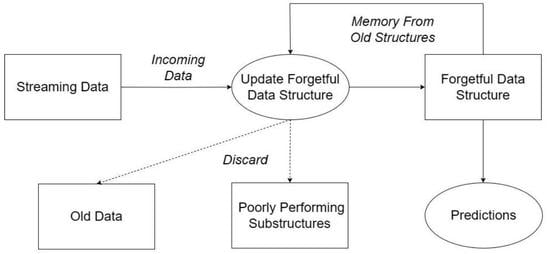
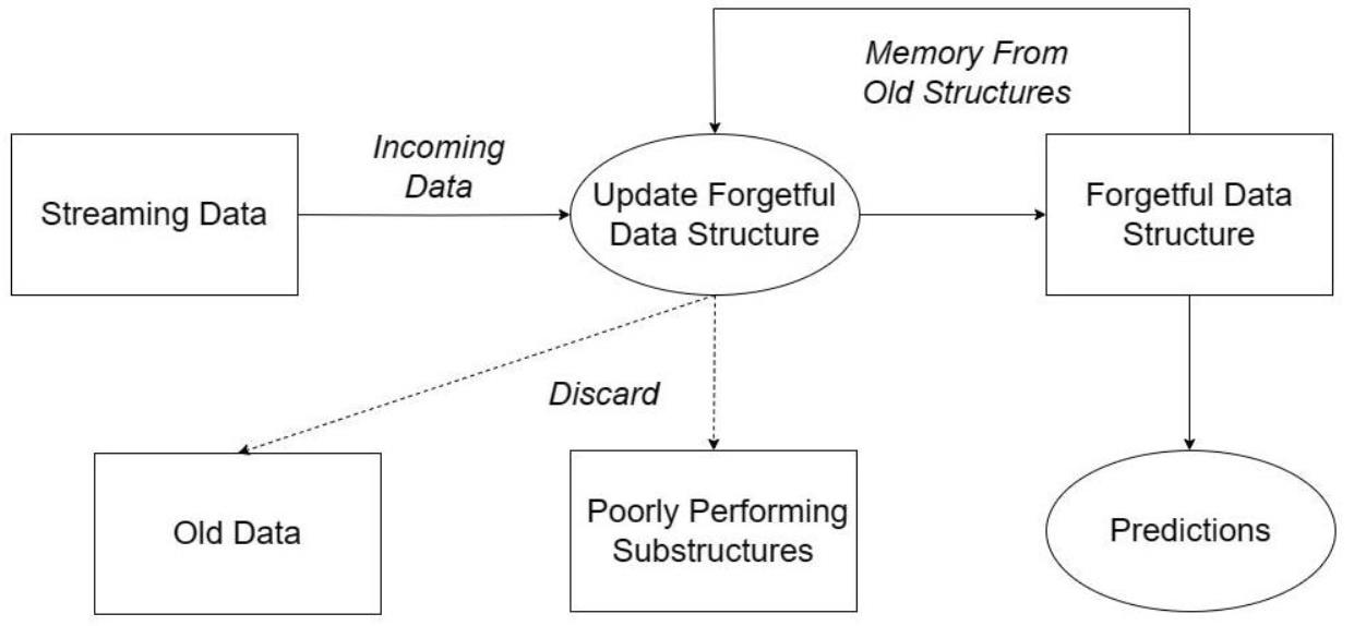
3. Forgetful Data Structures

This paper introduces both a forgetful decision tree and a forgetful random forest (having forgetful decision trees as components). These methods probabilistically forget old data and combine the retained old data with new data to track datasets that may undergo concept drift. In the process, the values of several hyperparameters are adjusted depending on the relative accuracy of the current model.
Given an incoming data stream, our method (i) saves time by maintaining the sorted order on each input attribute, (ii) efficiently rebuilds subtrees to process only incoming data whenever possible (i.e., whenever a split condition does not change). This works for both trees and forests, but because forests subsample the attributes, efficient rebuilding is more likely for forests.
To handle concept drift, we use three main ideas: (i) when the accuracy decreases, discard more of the older data and discard trees that have poor accuracy; (ii) when the accuracy increases, retain more old data; and (iii) vary the depth of the decision trees based on the size of the retained data.
The accuracy value in this paper is measured based on the confusion matrix: the proportion of true positive plus true negative instances relative to all test samples:
T r u e P o s i t i v e ~ i n ~ t e s t s e t + T r u e N e g a t i v e ~ i n ~ t e s t s e t S i z e t e s t s e t

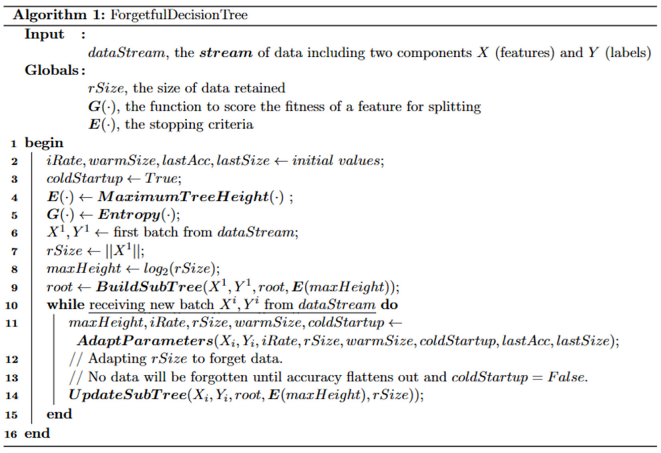
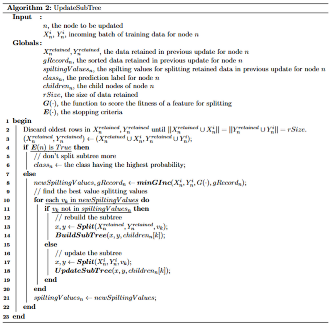
3.1. Forgetful Decision Trees

When a new incoming data batch is acquired from the data stream, the entire decision tree will be incrementally updated from the root node to the leaf nodes. The basic idea of this routine is to retain an amount of old data determined by an accuracy-dependent parameter called r S i z e (set in the routine Adapt Parameters). Next, the forgetful decision tree is rebuilt recursively but avoids rebuilding the subtree of any node n when the splitting criterion on n does not change. In that case, the subtree is updated rather than rebuilt. Updating entails only sorting the incoming data batch and placing it into the tree, while rebuilding entails sorting the new data with retained data and rebuilding the subtree. When the incoming batch is small, updating is much faster than rebuilding. Please see the detailed pseudocode and its explanation in Appendix A.

3.2. Adaptive Calculation of Retain Size and Max Tree Height

Retaining a substantial amount of historical data will result in higher accuracy when there is no concept drift, because the old information is useful. When concept drift occurs, r S i z e (the retained data) should be small, because old information will not reflect the new concept (which is some new mapping from input to label). Smaller r S i z e will result in increased speed. Thus, changing r S i z e can improve accuracy and reduce time. We use the following rules:
  • When accuracy increases (i.e., the more recent predictions have been more accurate than previous ones) a lot, the model can make good use of more data. We want r S i z e to increase with the effect so that we discard little or no data. When the accuracy increase is mild, the model has perhaps achieved an accuracy plateau, so we increase r S i z e , but only slightly.
  • When accuracy changes little or not at all, we allow r S i z e to slowly increase.
  • When accuracy decreases, we want to decrease r S i z e to forget old data, because this indicates that concept drift has happened. When concept drift is mild and accuracy decreases only a little, we want to retain more old data, so r S i z e should decrease only a little. When accuracy decreases a lot, the new data may follow a completely different functional mapping from the old data, so we want to forget most of the old data, suggesting r S i z e should be very small.
To achieve the above requirements, we adaptively change r S i z e . Besides that, we also adaptively change the maximum height of the tree ( m a x H e i g h t ). To avoid overfitting or underfitting, we will set m a x H e i g h t to be monotonic with r S i z e . In addition, to handle the cold start at the very beginning, we will not forget any data until more than a certain size of data (call it w a r m S i z e ) has arrived. We explain the details of adaptive parameters in Appendix B.

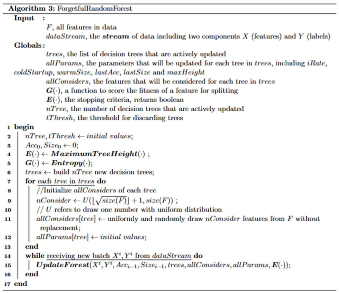
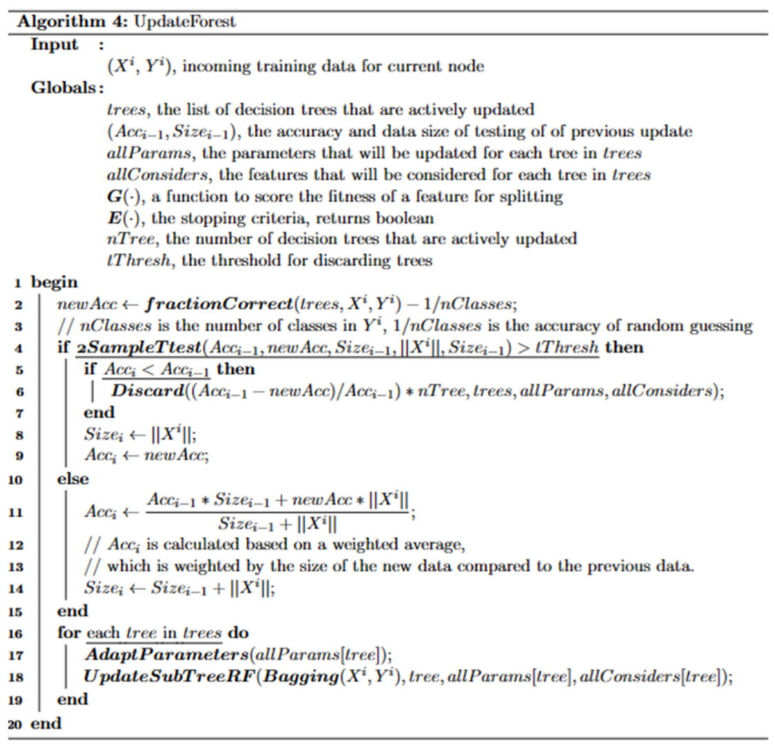
3.3. Forgetful Random Forest

The forgetful random forest is based on the forgetful decision tree described above in Section 3.1. Each random forest contains n T r e e forgetful decision trees. The update and rebuild algorithms for each decision tree in the random forest are the same as those described in Section 3.1 except:
  • Only a limited number of features are considered at each split, increasing the chance of updating (rather than rebuilding) subtrees during recursion, thus saving time by avoiding the need to rebuild subtrees from scratch. The number of features considered by each decision tree is uniformly and randomly chosen within the range ( n F e a t u r e s + 1 , n F e a t u r e s ] , where n F e a t u r e s is the number of features in the dataset. Further, every node inside the same decision tree considers the same features.
  • The update function for each tree will randomly and uniformly discard old data without replacement, instead of discarding data based on time of insertion. Because this strategy does not give priority to newer data, this strategy increases the diversity of the data given to the trees.
  • To decrease the correlation between trees and increase the diversity in the forest, we give the user the option to choose the leveraging bagging [11] strategy to the data arriving at each random forest tree. The size of the data after bagging is W times the size of original data, where W is a random number with an expected value of 6 , generated by a P o i s s o n λ = 6 distribution. To avoid the performance loss resulting from too many copies of the data, we never allow W to be larger than 10 . Each data item in the expanded data is randomly and uniformly selected from the original data with replacement. We apply bagging to each decision tree inside the random forest.
When the overall random forest accuracy decreases, our method discards trees that suffer from particularly poor performance. If the decrease is large, then forgetful random forests discard many trees. If the decrease is small, then our method discards fewer. The discarded trees will be replaced with the same data but different features. We will not discard any tree unless we have enough confidence (which is 1 t T h r e s h ) that the accuracy has decreased based on a two-sample t-test. The detailed pseudocode and accompanying explanation of the forgetful random forests are in Appendix C.

4. Tuning the Values of the Hyperparameters

Forgetful decision trees and random forests have six hyperparameters to set, which are (i) the evaluation function G of the decision tree, (ii) the maximum height of trees m a x H e i g h t , (iii) the minimum size of retained data following initial cold start w a r m S i z e , (iv) for forgetful random forests, the empirical probability that concept drift has occurred 1- t T h r e s h , (v) the number of trees in the forgetful random forest n T r e e , and (vi) the change in the retained data size i R a t e . To find the best values for these hyperparameters, we generated 18 datasets with different intensity of concept drifts, number of concept drifts, and Gaussian noise, using a generator inspired by Harvard Dataverse [16].
Our tests on the 18 new datasets indicated that some hyperparameters have optimal values (with respect to accuracy) that apply to all datasets. Others have optimal values that vary slightly depending on the dataset but can be learned. While the details are in Appendix D, here are the results of that study:
  • The evaluation function can be a Gini Impurity [17] score or an entropy reduction coefficient. Which one is chosen does not make a material difference, so we set G to entropy reduction coefficient for all datasets.
  • The maximum tree height ( m a x H e i g h t ) is adaptively set based on the methods in Section 3.2 to log base 2 of r S i z e . Applying other stopping criteria does not materially affect the accuracy. For that reason, we ignore other stopping criteria.
  • To mitigate the inaccuracies of the initial cold start, the model will not discard any data in cold startup mode. To leave cold startup mode, the accuracy should be better than random guessing on the last 50 % of data, when r S i z e is at least w a r m S i z e . w a r m S i z e adapts if it is too small, so we will set its initial value to 64 data items.
  • To avoid discarding trees too often, we will discard a tree only when we have 1 t T h r e s h confidence that the accuracy has changed. We observe that all datasets enjoy a good accuracy when t T h r e s h = 0.05 .
  • There are n T r e e forgetful decision trees in each forgetful random forest. We observe that the accuracy of all datasets stops growing after n T r e e > 20 both with bagging and without bagging, so we will set n T r e e = 20 .
  • The adaptation strategy in Section 3.2 needs an initial value for parameter i R a t e , which influences the increase rate of the retained data r S i z e . Too much data will be retained if the initial i R a t e is large, but the accuracy will be low for lack of training data if the initial value of i R a t e is small. We observe that the forgetful decision tree does well when i R a t e = 0.3 or i R a t e = 0.4 initially. We will use i R a t e = 0.3 as our initial setting and use it in the experiments of Section 5 for all our algorithms, because most simulated datasets have higher accuracy at i R a t e = 0.3 than at i R a t e = 0.4 .

5. Results

This section compares the following algorithms: forgetful decision tree, forgetful random forest with bagging, forgetful random forest without bagging, Hoeffding Tree [8,18], Hoeffding adaptive tree [12], iSOUP tree [9], train once, and adaptive random forest [14]. The forgetful algorithms use the hyperparameter settings from Section 4 on both the real datasets and the synthetic datasets produced by others.
We measure time consumption, the accuracy and, where appropriate, the F1 score.
The following settings yield the best accuracy for the state-of-the-art algorithms with which we compare:
  • Previous papers [8,18] provide two different configurations for the Hoeffding tree. The configuration from [8] usually has the highest accuracy, so we will use it in the following experiment: s p l i t _ c o n f i d e n c e = 10 7 , g r a c e _ p e r i o d = 200 , and t i e _ t h r e s h o l d = 0.05 . Because the traditional Hoeffding tree cannot deal with concept drift, we set l e a f _ p r e d i c t i o n = N a i v e   B a y e s   A d a p t i v e to allow the model to adapt when concept drift happens.
  • The designers of the Hoeffding adaptive tree suggest six possible configurations of the Hoeffding adaptive tree, which are HAT-INC, HATEWMA, HAT-ADWIN, HAT-INC NB, HATEWMA NB, and HAT-ADWIN NB. HAT-ADWIN NB has the best accuracy, and we will use it in the following experiments. The configuration is l e a f _ p r e d i c t i o n = N a i v e   B a y e s , s p l i t _ c o n f i d e n c e = 0.0001 , g r a c e _ p e r i o d = 200 , and t i e _ t h r e s h o l d = 0.05 .
  • The designers provide only one configuration for the iSOUP tree [9], so we will use it in the following experiment. The configuration is l e a f _ p r e d i c t i o n = a d a p t i v e , s p l i t _ c o n f i d e n c e = 0.0001 , g r a c e _ p e r i o d = 200 , and t i e _ t h r e s h o l d = 0.05 .
  • For the train-once model, we will train the model only once with all of the data before starting to measure accuracy and other metrics. The train-once model is never updated again. In this case, we will use a non-incremental decision tree, which is the CART algorithm [7], to fit the model. We use the setting with the best accuracy, which is c r i t e r i o n = g i n i , and no other restrictions.
The designers of adaptive random forest provided six variant configurations of adaptive random forest [14]: the variants A R F m o d e r a t e , A R F f a s t , A R F P H T , A R F n o B k g , A R F s t d R F , and A R F m a j . A R F f a s t has the highest accuracy in most cases that we tested, so we will use that configuration: δ w = 0.01 , δ d = 0.001 , and l e a r n e r s = 100 .

5.1. Categorical Variables

Because the real datasets all contain categorical variables and the forgetful methods do not handle those directly, we modified the categorical variables into their one-hot encodings using the OneHotEncoder of scikit-learn [19]. For example, a categorical variable c o l o r = { R , G , B } will be transferred to three binary variables i s R = { T r u e , F a l s e } , i s G = { T r u e , F a l s e } , and i s B = { T r u e , F a l s e } . In addition, all of the forgetful methods in the following tests use only binary splits at each node.

5.2. Metrics

In addition to accuracy, we use precision, r e c a l l , and F1 score to evaluate our methods. Precision and recall are appropriate to problems where there is a class of interest, and the question is which percentage of predictions of that class are correct (precision) and how many instances of that class are predicted (recall). This is appropriate for the detection of phishing websites. Accuracy is more appropriate in all other applications. For example, in the electricity datasets, price up and price down are both classes of interest. Therefore, we present precision, recall, and the F1 score for phishing only. We use the following formula based on the confusion matrix:
  • a c c u r a c y = T r u e P o s i t i v e + T r u e N e g a t i v e S i z e t e s t s e t
  • p r e c i s i o n = T r u e P o s i t i v e T r u e P o s i t i v e + F a l s e P o s i t i v e
  • r e c a l l = T r u e P o s i t i v e T r u e P o s i t i v e + F a l s e N e g a t i v e
  • F 1 s c o r e = 2 T r u e P o s i t i v e 2 T r u e P o s i t i v e + F a l s e N e g a t i v e + F a l s e P o s i t i v e
In contrast to i.i.d. machine learning tasks, we do not partition the data into a training set and a test set. Instead, when each batch of data arrives, we measure the accuracy and F1 score of the predictions on that batch, before we use the batch to update the models.
We start measuring accuracy and F1 score after the accuracy of the forgetful decision tree flattens out, in order to avoid evaluating the predictions during initial start-up when too little data has arrived to create a good model. For each dataset, all algorithms (state-of-the-art and forgetful) will start measuring the accuracy and F1 score after the same amount of data has arrived.

5.3. Datasets

We use four real datasets and two synthetic datasets to test the performance of our forgetful methods against the state-of-the-art incremental algorithms. The forest cover type, phishing, and power supply datasets suffer from frequent and mild concept drifts, the electricity dataset suffers from frequent and drastic concept drift, and the two synthetic datasets suffer from gradual and abrupt concept drifts, respectively. Thus, our test datasets cover a variety of concept drift scenarios.
  • The forest cover type (ForestCover) [20] dataset captures images of forests for each 30 30 m cell determined from the US Forest Service (USFS) Region 2 Resource Information System (RIS) data. Each increment consists of 400 image observations. The task is to infer the forest type. This dataset suffers from concept drift because later increments have different mappings from input image to forest type than earlier ones. For this dataset, the accuracy first increases and then flattens out after the first 24,000 data items have been observed, out of 581,102 data items.
  • The electricity [21] dataset describes the price and demand of electricity. The task is to forecast the price trend in the next 30 min. Each increment consists of data from one day. This data suffers from concept drift because of market and other external influences. For this dataset, the accuracy never stabilizes, so we start measuring accuracy after the first increment, which is after the first 49 data items have arrived, out of 36,407 data items.
  • Phishing [22] contains 11,055 web pages accessed over time, some of which are malicious. The task is to predict which pages are malicious. Each increment consists of 100 pages. The tactics of phishing purveyors get more sophisticated over time, so this dataset suffers from concept drift. For this dataset, the accuracy flattens out after the first 500 data items have arrived.
  • Power supply [23] contains three years of power supply records of an Italian electrical utility, comprising 29,928 data items. Each data item contains two features, which are the amount of power supplied from the main grid and the amount of power transformed from other grids. Each data item is labelled with the hour of the day when it was collected (from 0 to 23 ). The task is to predict the label from the power measurements. Concept drift arises because of season, weather, and the differences between working days and weekends. Each increment consists of 100 data items, and the accuracy flattens out after the first 1000 data items have arrived.
  • The two synthetic datasets are from [16]. Both are time-ordered and are designed to suffer from concept drift over time. One, called Gradual, has 41,000 data points. Gradual is characterized by complete label changes that happen gradually over 1000 data points at three single points, and 10,000 data items between each concept drift. Another dataset, called Abrupt, has 40,000 data points. It undergoes complete label changes at three single points, with 10,000 data items between each concept drift. Each increment consists of 100 data points. Unlike the datasets that were used in Section 4, these datasets contain only four features, two of which are binary classes without noise, and the other two are sparse values generated by s i n x and s i n 1 y , where x and y are the uniformly generated random numbers. For both datasets, the accuracy flattens out after 1000 data items have arrived.
To measure the statistical stability in the face of the noise caused by the randomized setting of the initial seeds, we test all decision trees and random forests six times with different seeds and record the mean values with a 95 % confidence interval for time consumption, accuracy, and F1 score.
The following experiments are performed on an Intel Xeon Platinum 8268 24C 205W 2.9 GHz Processor with 200 gigabytes of memory, Intel, Santa Clara, CA, USA.

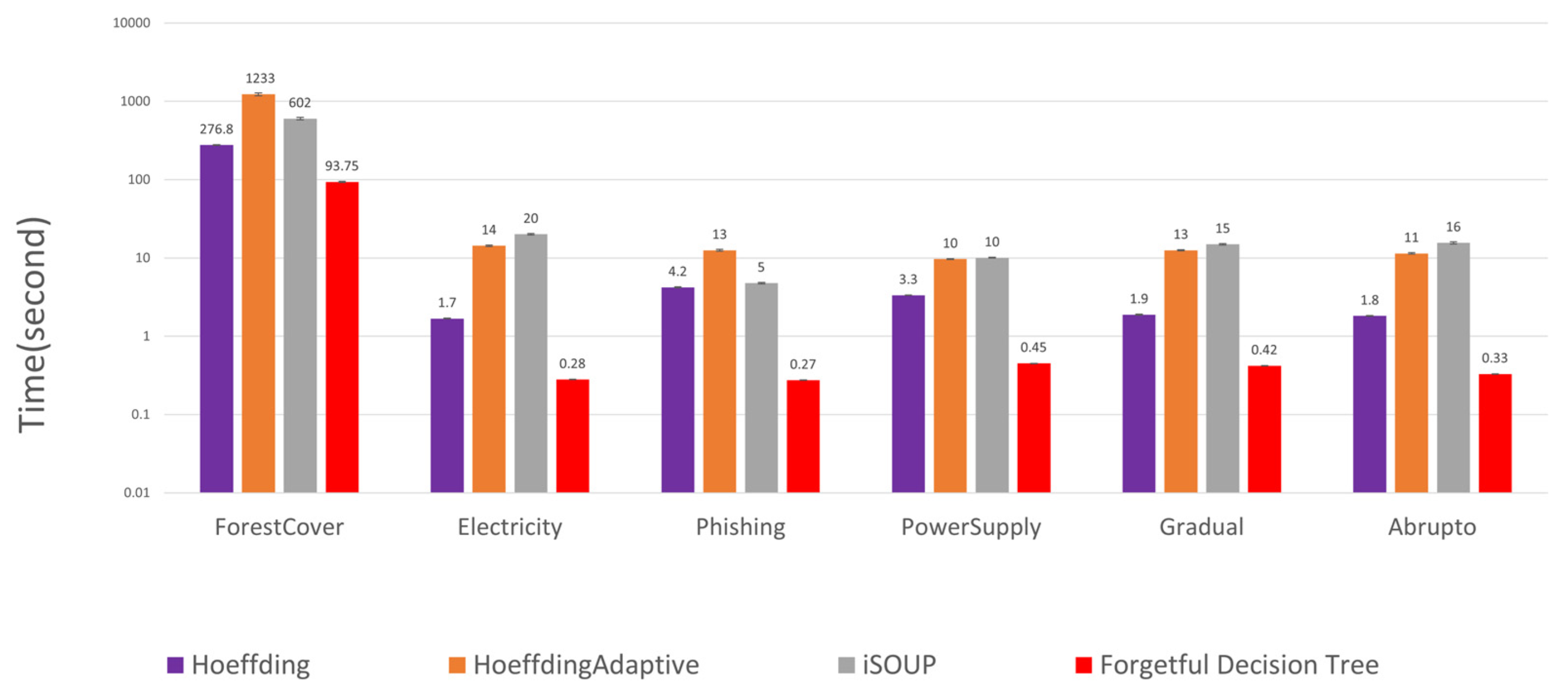
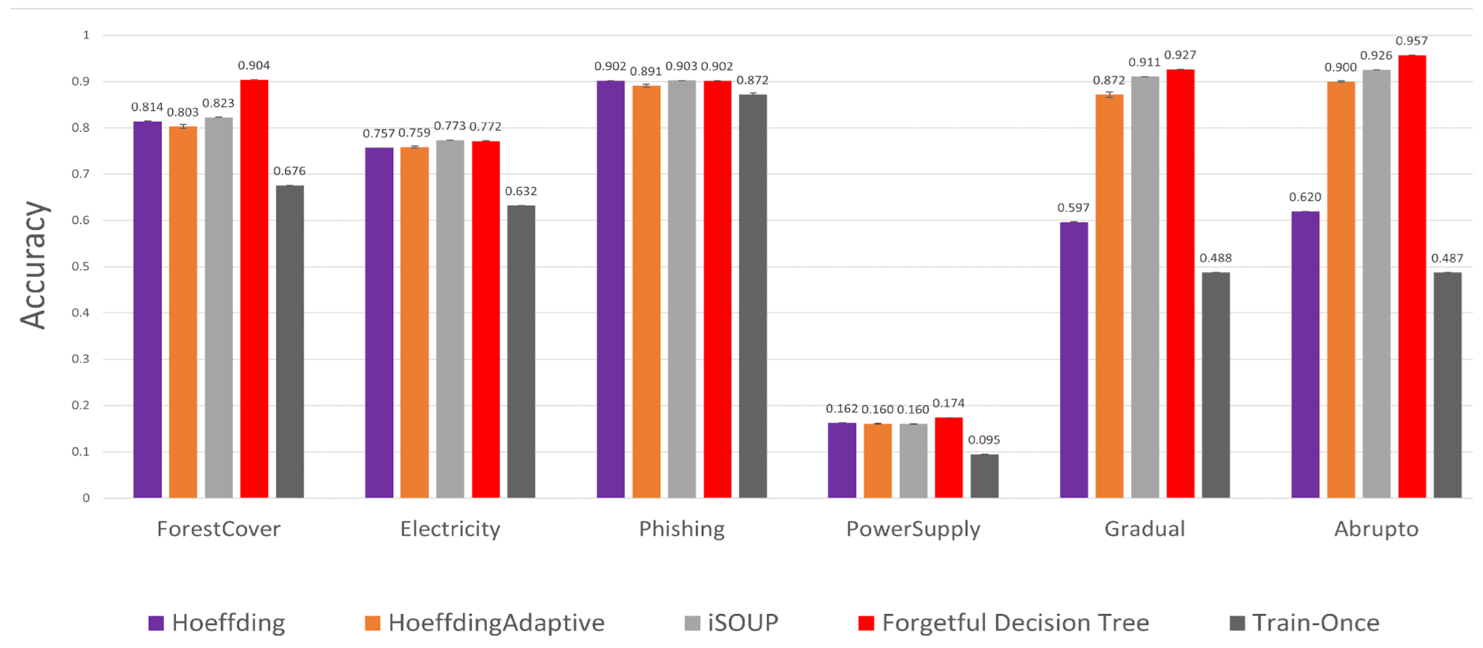
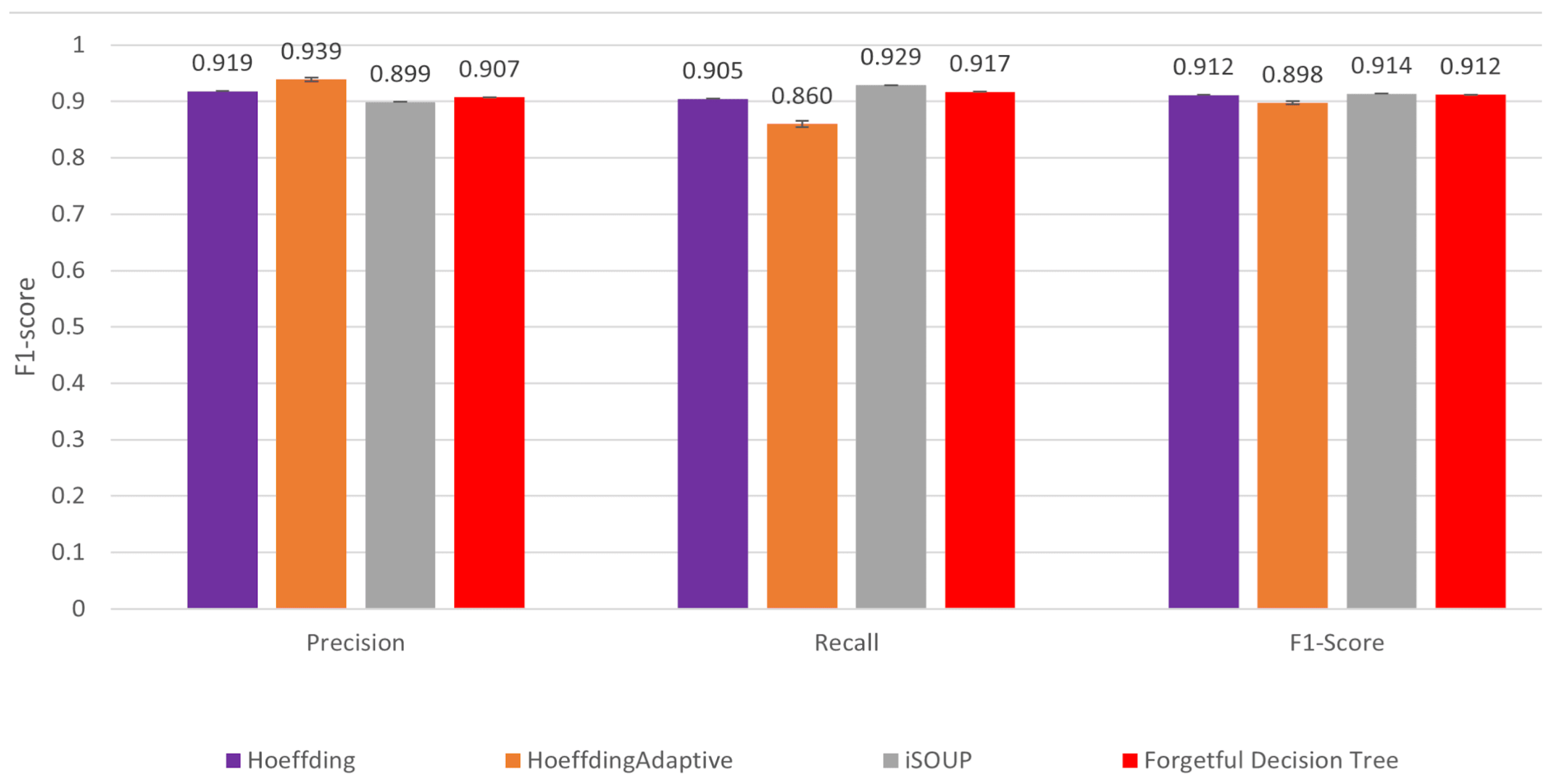
5.4. Quality and Time Performance of the Forgetful Decision Tree

Figure 1 compares the time consumption of different incremental decision trees. For all datasets, the forgetful decision tree is at least three times faster than the other incremental methods.
Figure 2 compares the accuracy of different incremental decision trees and a train-once model. For all datasets, the forgetful decision tree is as accurate or more accurate than other incremental methods.
Figure 3 compares the precision, recall, and F1 score of different incremental decision trees. Because these metrics are not appropriate for other datasets, we use them only on the phishing dataset. The precision and recalls vary. For example, the Hoeffding adaptive tree has a better precision but a worse recall than the forgetful decision tree, while the iSOUP tree has a better recall but a worse precision. Overall, the forgetful decision tree has a similar F1 score to the other incremental methods.

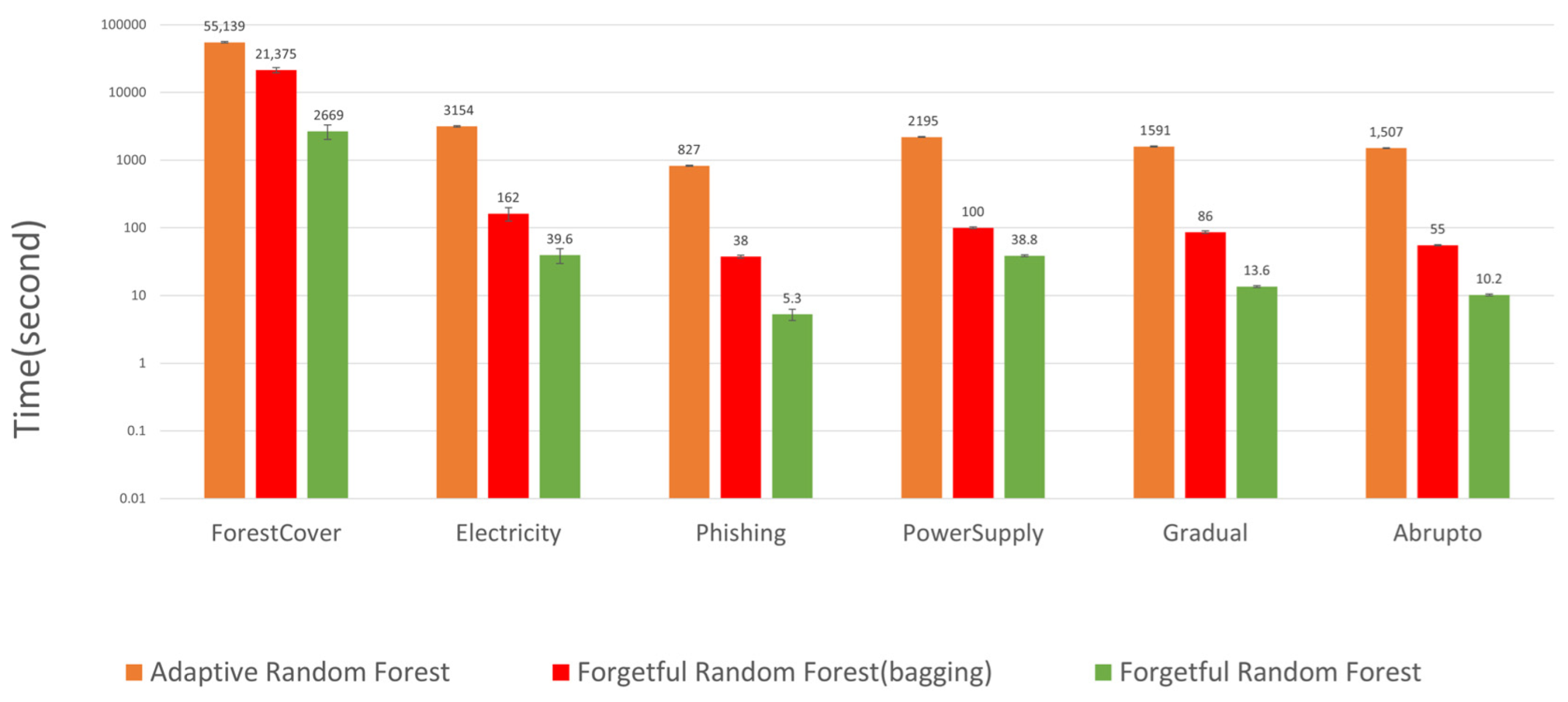
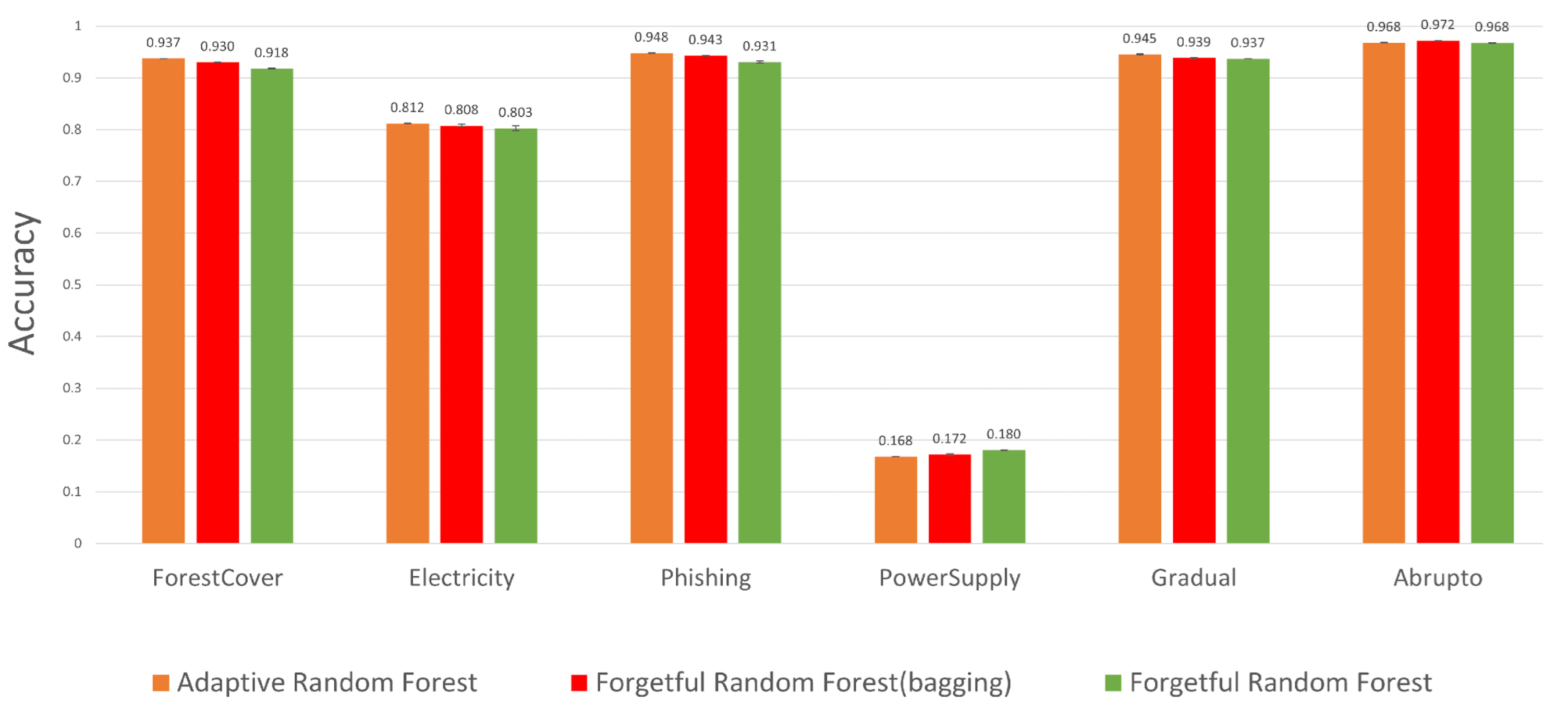
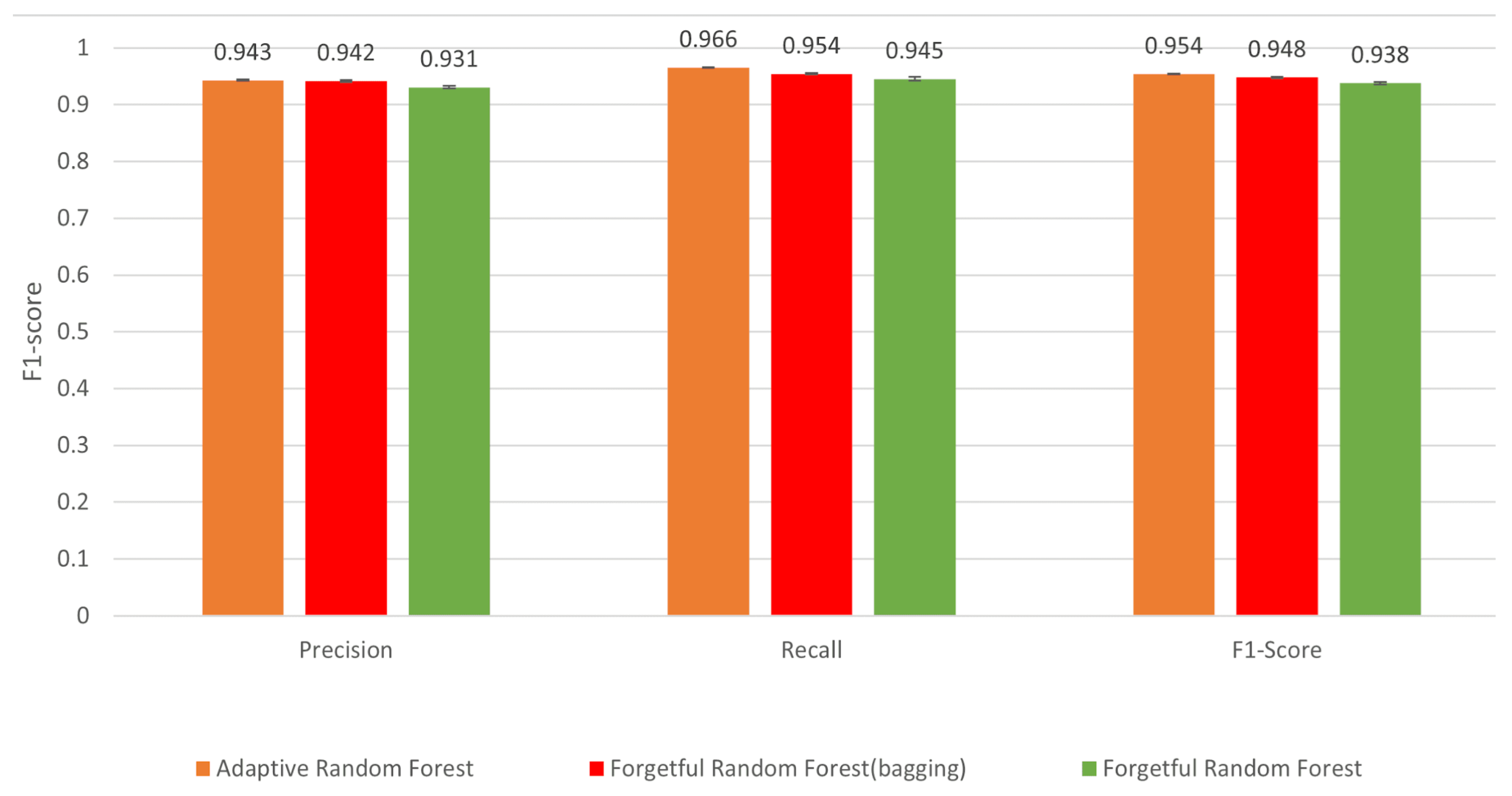
5.5. Quality and Time Performance of the Forgetful Random Forest

Figure 4 compares the time performance of maintaining different random forests. From this figure, we observe that the forgetful random forest without bagging is the fastest algorithm. In particular, it is at least 24 times faster than the adaptive random forest. The forgetful random forest with bagging is about 10 times slower than without bagging, but it is still 2.5 times faster than the adaptive random forest.
Figure 5 compares the accuracy of different random forests. From these figures, we observe that the forgetful random forest without bagging is slightly less accurate than the adaptive random forest (by at most 2 % ). By contrast, the forgetful random forest with bagging has a similar accuracy compared to the adaptive random forest. For some applications, the loss of accuracy might be acceptable in order to handle a high streaming data rate.
Figure 6 compares the precision, recall, and F1 score of training different random forests when these evaluations are appropriate. From these figures, we observe that the forgetful random forest without bagging has a lower precision, recall, and F1 score than the adaptive random forest (by at most 0.02 ). By contrast, the forgetful random forest with bagging has a similar precision but a lower recall and F1 score (by at most 0.01 ) compared to the adaptive random forest.

6. Discussion and Conclusions

Forgetful decision trees and forgetful random forests constitute simple, fast and accurate incremental data structure algorithms. We have found that:
  • The forgetful decision tree is at least three times faster and at least as accurate as state-of-the-art incremental decision tree algorithms for a variety of concept drift datasets. When the precision, recall, and F1 score are appropriate, the forgetful decision tree has a similar F1 score to state-of-the-art incremental decision tree algorithms.
  • The forgetful random forest without bagging is at least 24 times faster than state-of-the-art incremental random forest algorithms, but is less accurate by at most 2 % .
  • By contrast, the forgetful random forest with bagging has a similar accuracy to the most accurate state-of-the-art forest algorithm (adaptive random forest) and is 2.5 faster.
  • At a conceptual level, our experiments show that it was possible to set hyperparameter values based on changes in accuracy on synthetic data and then apply those values to real data. The main such hyperparameters are i R a t e (increase rate of size of data retained), t T h r e s h (the confidence interval that accuracy has changed), and n T r e e (the number of decision trees in the forgetful random forests).
  • Further our experiments show the robustness of our approach across a variety of applications where concept drift is frequent or infrequent, mild or drastic, and gradual or abrupt.
In summary, forgetful data structures speed up traditional decision trees and random forests for streaming data and help them adapt to concept drift. Further, bagging increases accuracy but at some cost in speed. The most pressing question for future work is whether some alternative method to bagging can be combined with forgetfulness to increase accuracy at less cost in a streaming concept drift setting.

Author Contributions

Conceptualization, Z.Y. and D.S.; methodology, Z.Y.; software, Z.Y.; validation, Z.Y. and Y.S.; formal analysis, Z.Y.; investigation, Z.Y.; resources, Z.Y. and D.S.; data curation, Z.Y.; writing—original draft preparation, Z.Y., Y.S. and D.S.; writing—review and editing, Z.Y., Y.S. and D.S.; visualization, Z.Y.; supervision, D.S.; project administration, D.S.; funding acquisition, D.S. All authors have read and agreed to the published version of the manuscript.

Funding

The authors would like to acknowledge the support of the U.S. National Science Foundation grants 1840761, 1934388, and 1840761, the U.S. National Institutes of Health grant 5R01GM121753 and NYU Wireless.

Data Availability Statement

Publicly available datasets were analyzed in this study. This data and our code can be found here: https://github.com/ZhehuYuan/Forgetful-Random-Forest.git (accessed on 25 May 2023).

Conflicts of Interest

The authors declare no conflict of interest.

Appendix A. Algorithms for Forgetful Decision Trees

Figure A1. Main function of the forgetful decision tree. | | X | | refers to the number of rows in batch X . Notice that coldStartup occurs only when data first appears. There are no further cold starts after concept drifts.
Algorithms 16 00278 g0a1
Figure A2. UpdateSubTree algorithm. It recursively concatenates the retained old data with the incoming data and uses that data to update the best splitting points or prediction label for each node. Note that the split on line 17 is likely to be less expensive than the split on line 13.
Algorithms 16 00278 g0a2
The forgetful decision tree main routine (Figure A1) is called on the initial data and each time a new batch (an incremental batch) of data is received. The routine will make predictions with the tree before the batch and then update the batch. To avoid measuring accuracy during cold start, accuracy results are recorded only after the accuracy flattens out (i.e., when the accuracy changes 10 % or less between the last 500 data items and the previous 500 data items). B u i l d S u b T r e e and U p d a t e S u b T r e e are called by the main routine. The B u i l d S u b T r e e (not shown) is essentially the original CART build algorithm, and the U p d a t e S u b T r e e is designed as follows:
  • The stopping criteria E may combine one or more factors, such as maximum tree height, minimum samples to split, and minimum impurity decrease. If the criteria holds, then the node will not further split. In addition, if all data points in the node have the same label, that node will not be split further. m a x H e i g h t controls E and is computed in A d a p t P a r a m e t e r s ( . ) below.
  • The evaluation function G evaluates the splitting score for each feature and each splitting value. It will typically be a Gini Impurity [17] score or an entropy reduction coefficient. As we discuss below, the functions m i n G and m i n G I n c find split points that minimize the weighted sum of scores of each subset of the data after splitting. Thus, the score must be evaluated on many split points (e.g., if the input attribute is a g e , then possible splitting criteria could be a g e > 30 , a g e > 32 , …) to find the optimal splitting values.
  • r S i z e determines the size of X n r e t a i n e d X n i and Y n r e t a i n e d Y n i to be retained when new data for X and Y arrives. For example, suppose r S i z e = 100 . Then | | X n i | | + | | X n r e t a i n e d | | 100 of the oldest of X n r e t a i n e d and Y n r e t a i n e d (the data present before the incoming batch) will be discarded. The algorithm then appends X n i and Y n i to what remains of X n r e t a i n e d and Y n r e t a i n e d . All nodes in the subtrees will discard the same data items as the root node. In this way, the tree is trained with only the newest r S i z e of data in the tree. Discarding old data helps to overcome concept drift, because the newer data better reflects the mapping from X to Y after concept drift. r S i z e should never be less than | | X n i | | , to avoid forgetting any new incoming data. As mentioned above, upon initialization, new data will be continually added to the structure without forgetting until accuracy flattens out, which is controlled by c o l d S t a r t u p . r S i z e and c o l d S t a r t u p are computed in A d a p t P a r a m e t e r s ( . ) below.
After the retained old data is concatenated with the incoming batch data, the decision tree is updated in a top-down fashion using the U p d a t e S u b T r e e . function (Figure A2) based on G . .
At every interior node, function m i n G I n c . calculates a score for every feature by evaluating function G on the data allocated to the current node. This calculation leads to the identification of the best feature and best value (or potentially values) to split on, with the result that the splitting gives rise to two or more splitting values for a feature. The data discarded in line 2 of U p d a t e S u b T r e e . will not be considered by m i n G I n c . . If, at some node, the best splitting value (or values) is different from the choice before the arrival of the new data, the algorithm rebuilds the subtree with the data retained as well as the new data allocated to this node (the B u i l d S u b T r e e . function). Otherwise, if the best splitting value (or values) is the same as the choice before the arrival of the new data, the algorithm splits only the incoming data among the children and then recursively calls the U p d a t e S u b T r e e . function on these child nodes.
In summary, the forgetting strategy ensures that the model is trained only on the newest r S i z e data. The rebuilding strategy determines whether a split point can be retained in which case tree reconstruction is vastly accelerated using U p d a t e S u b T r e e . . Even if the unshown B u i l d S u b T r e e . is used, the calculation of the split point based on G . (e.g., Gini score) is somewhat accelerated because the relevant data is already nearly sorted.

Appendix B. Ongoing Parameter Tuning

We use the A d a p t P a r a m e t e r s . function to adaptively change c u r r e n t P a r a m s . r S i z e , m a x H e i g h t , and c u r r e n t P a r a m s . i R a t e based on changes in accuracy. A d a p t P a r a m e t e r s . is called when new data is acquired from the data stream and before function U p d a t e S u b T r e e . is called. The r S i z e and m a x H e i g h t will be applied to the parameters when calling U p d a t e S u b T r e e . . The i R a t e and r S i z e will also be inputs to the next call to the A d a p t P a r a m e t e r s . function on this tree.
The A d a p t P a r a m e t e r s . function will first test the accuracy of the model on new incoming data yielding n e w A c c . The function then recalls the accuracy that was tested last time as l a s t A c c . Next, because we want n e w A c c and l a s t A c c to improve upon random guessing, we subtract the accuracy of random uniform guessing from n e w A c c (the g u e s s A c c was already subtracted from l a s t A c c in the last update). We posit that the accuracy of random guessing ( g u e s s A c c ) to be 1 / n C l a s s e s . The intuitive reason to subtract g u e s s A c c is that a l a s t A c c that is no greater than g u e s s A c c suggests that the model is no better than guessing just based on the number of classes. That, in turn, suggests that concept drift has likely occurred so old data should be discarded.
Following that, A d a p t P a r a m e t e r s . will calculate the rate of change ( r C h a n g e ) of r S i z e by:
  • When n e w A c c / l a s t A c c 1 , the m a x in the exponent will ensure that r C h a n g e will be n e w A c c / l a s t A c c 2 . In this way, the r C h a n g e curves slightly upward when n e w A c c is equal to, or slightly higher than l a s t A c c , but curves steeply upward when n e w A c c is much larger than l a s t A c c .
  • When n e w A c c / l a s t A c c < 1 , r C h a n g e is equal to n e w A c c / l a s t A c c 3 n e w A c c / l a s t A c c . In this way, r C h a n g e is flat or curves slightly downward when n e w A c c is slightly lower than l a s t A c c but curves steeply downwards when n e w A c c is much lower than l a s t A c c .
  • Other functions to set r C h a n g e are possible, but this one has the following desirable properties: (i) it is continuous regardless of the values of n e w A c c and l a s t A c c ; (ii) r C h a n g e is close to 1 when n e w A c c is close to l a s t A c c ; (iii) when n e w A c c differs from l a s t A c c significantly in either direction, r C h a n g e reacts strongly.
Numbered lists can be added. Finally, we will calculate and update the new r S i z e by multiplying the old r S i z e by r C h a n g e . To effect a slow increase in c u r r e n t P a r a m s . r S i z e when n e w A c c l a s t A c c and r C h a n g e 1 , we increase r S i z e by i R a t e | | X n | | in additional to r S i z e o l d r C h a n g e , where i R a t e (the increase rate) is a number that is maintained from one call to A d a p t P a r a m e t e r s . to another. The size of the incoming data is | | X n i | | , so r S i z e cannot increase by more than | | X n i | | . In addition, we do not allow r S i z e to be less than | | X n i | | , because we do not want to forget any new incoming data. When A d a p t P a r a m e t e r s . is called the first time, we will set r S i z e = | | X n i | | + | | X n r e t a i n e d | | .
The two special cases happen when n e w A c c 0 or l a s t A c c 0 . When n e w A c c 0 , the prediction of the model is no better than random guessing. In that case, we infer that the old data cannot help in predicting new data, so we will forget all of the old data by setting r S i z e = | | X n i | | . When l a s t A c c 0 but n e w A c c > 0 , then all the old data may be useful. Thus, we set r S i z e = r S i z e + | | X n i | | .
The above adaptation strategy requires a dampening parameter i R a t e to limit the increase rate of r S i z e . When the accuracy is large, the model may be close to its maximum possible accuracy, so we may want a smaller i R a t e and in turn to increase r S i z e slower. After a drastic concept drift event, when the accuracy has been significantly decreased, we want to increase i R a t e to retain more new data after forgetting most of the old data. This will accelerate the creation of an accurate tree after the concept drift. To achieve this, we will adaptively change it as follows: set i R a t e   n e w equal to i R a t e o l d l a s t A c c / n e w A c c before each update to r S i z e . i R a t e will not be changed if either l a s t A c c 0 or n e w A c c 0 .
Upon initialization, if the first increment is small, then n e w A c c may not exceed 1 / n C l a s s e s , and the model will forget all of the old data every time. To avoid such poor performance at cold start, the forgetful decision tree will be initialized in cold startup mode. In cold startup mode, the forgetful decision tree will not forget any data. When r S i z e reaches w a r m S i z e , the forgetful decision tree will leave cold startup mode if n e w A c c is better than g u e s s A c c since the last 50 % data arrived. Otherwise, w a r m S i z e will be doubled. The above process will be repeated until leaving cold startup mode.
Max tree height is closely related to the size of data retained in the tree. We want each leaf node to have about one data item on average when the tree is perfectly balanced, so we always set m a x H e i g h t = l o g 2 r S i z e .

Appendix C. Algorithms for Forgetful Random Forests

Figure A3. Main function of the forgetful random forest. The value n C o n s i d e r is the size of the subset of features considered for any given tree.
Algorithms 16 00278 g0a3
Figure A4. UpdateForest algorithm. This routine discards and rebuild trees when accuracy decreases and then (optionally) updates each tree with bagged incoming data.
Algorithms 16 00278 g0a4
As for the forgetful decision tree main routine, the forgetful random forest main routine (Figure A3) is called initially and then each time an incremental batch of data is received. The routine will make predictions with the random forest before the batch and then update the random forest. The main function of forgetful random forest describes only the update part. Accuracy results apply after the accuracy flattens out to avoid measuring accuracy during initial cold start. Flattening out occurs when the accuracy changes 10% or less between the last 500 data items and the previous 500 data items. U p d a t e F o r e s t R F . function will be called by the main routine to incrementally update the forest. The U p d a t e F o r e s t R F . function is the same as the U p d a t e F o r e s t . function except only features in a l l C o n s i d e r s [ t r e e ] are considered.
In addition to updating each tree inside the forest, updating the random forest also includes discarding the trees with features that perform poorly after concept drift (Figure A4). To achieve that, we will call the D i s c a r d . function (explained below) when n e w A c c is significantly less than A c c i 1 . As in the U p d a t e F o r e s t . function, we will subtract the accuracy of randomly and uniformly guessing one class out of nClasses from n e w A c c and from A c c i 1 to show the improvement of the model with respect to random guessing. Significance is based on a p v a l u e test: the accuracy of the forest has changed with a p v a l u e < t T h r e s h based on a 2-sample t-test. The variable t T h r e s h is a hyper-parameter that will be tuned in Section 4 and Appendix D.
To detect slight but continuous decreases in accuracy, we will calculate A c c i and S i z e i by the weighted average calculation in the pseudo-code when the change in accuracy is insignificant ( p v a l u e > t T h r e s h ). By contrast, when the change in accuracy is significant, we will set A c c i and S i z e i to n e w A c c and | | X i | | after the D i s c a r d . function is called.
The D i s c a r d . function removes the A c c i 1 n e w A c c / A c c i 1 n T r e e decision trees of the random forest having the least accuracy when evaluated on the new data. The discarded trees are replaced with new decision trees. Each new tree will take all the data from the tree it replaced, but the tree will be rebuilt, the a l l P a r a m s for that tree will be re-initialized, and the considered features will be re-selected for that tree. After building the new tree, the algorithm will test the tree on the latest data to calculate l a s t A c c and l a s t S i z e of the new tree. In this way, new trees adapt their r S i z e and i R a t e based on the newly arriving data.

Appendix D. Methods for Determining Hyperparameters

To find the best hyperparameters, we created 18 simulated datasets. Each dataset contains 50,000 data items labeled with { 0,1 } without noise. Each item is characterized by 10 binary features. Each dataset is labeled with C , I , where C means that it has C 1 uniformly distributed concept drifts, and I is the intensity of the concept drift, while a mild concept drift will drift one feature, a medium concept drift will drift three features, and a drastic concept drift will drift 5 features. In addition, for each dataset, we have one version without Gaussian noise and the other version with Gaussian noise ( λ = 0 , s t d = 1 , unit is the number of features). We tested the forgetful decision tree and forgetful random forest with different initial hyperparameter values on these synthetic datasets. We first set the evaluation function, maximum height function, and w a r m S i z e in advance, because these parameters do not materially affect the accuracy. Then we use exhaustive search on all possible combinations of the remaining three hyperparameters to find the best values for them. To measure statistical stability in the face of the noise caused by the random setting of the initial seeds, we tested the random forests six times with different seeds and recorded the average accuracies. In our test, all curves (variable values against accuracies) are flattened, and we choose the values that result in the best accuracy as our default hyperparameters.

References

  1. Pandey, R.; Singh, N.K.; Khatri, S.K.; Verma, P. Artificial Intelligence and Machine Learning for EDGE Computing; Elsevier Inc.: Amsterdam, The Netherlands, 2022; pp. 23–32. [Google Scholar]
  2. Saco, A.; Sundari, P.S.; J, K.; Paul, A. An Optimized Data Analysis on a Real-Time Application of PEM Fuel Cell Design by Using Machine Learning Algorithms. Algorithms 2022, 15, 346. [Google Scholar] [CrossRef]
  3. LeCun, Y.; Bengio, Y.; Hinton, G. Deep learning. Nature 2015, 521, 436–444. [Google Scholar] [CrossRef] [PubMed]
  4. Stuart Russell; Peter Norvig. Artificial Intelligence: A Modern Approach, 4th ed.; Prentice Hall: Hoboken, NJ, USA, 2020; pp. 1–36. [Google Scholar]
  5. Polikar, R.; Upda, L.; Upda, S.S.; Honavar, V. Learn++: An incremental learning algorithm for supervised neural networks. IEEE Trans. Syst. 2001, 31, 497–508. [Google Scholar] [CrossRef]
  6. Diehl, C.; Cauwenberghs, G. SVM incremental learning, adaptation and optimization. Proc. Int. Joint Conf. Neural Netw. 2003, 4, 2685–2690. [Google Scholar] [CrossRef]
  7. Loh, W.-Y. Classification and Regression Trees. WIREs Data Mining Knowl. Discov. 2011, 13, 14–23. [Google Scholar] [CrossRef]
  8. Sun, J.; Jia, H.; Hu, B.; Huang, X.; Zhang, H.; Wan, H.; Zhao, X. Speeding up Very Fast Decision Tree with Low Computational Cost. In Proceedings of the Twenty-Ninth International Joint Conference on Artificial Intelligence, Yokohama, Japan, 11–17 July 2020; Volume 7, pp. 1272–1278. [Google Scholar] [CrossRef]
  9. Osojnik, A.; Panov, P.; Dzeroski, S. Tree-based methods for online multi-target regression. J. Intell. Inf. Syst. 2017, 50, 315–339. [Google Scholar] [CrossRef]
  10. Domingos, P.; Hulten, G. Mining High-Speed Data Streams. In Proceedings of the Sixth ACM SIGKDD International Conference on Knowledge Discovery and Data Mining, Boston, MA, USA, 20–23 August 2000; KDD’00. Association for Computing Machinery: New York, NY, USA, 2000; pp. 71–80. [Google Scholar] [CrossRef]
  11. Hoeffding, W. Probability Inequalities for sums of Bounded Random Variables. In The Collected Works of Wassily Hoeffding; Springer Series in Statistics; Fisher, N.I., Sen, P.K., Eds.; Springer: New York, NY, USA, 1994. [Google Scholar]
  12. Bifet, A.; Gavaldà, R. Adaptive Learning from Evolving Data Streams. In Advances in Intelligent Data Analysis VIII; Adams, N.M., Robardet, C., Siebes, A., Boulicaut, J.-F., Eds.; Springer: Berlin/Heidelberg, Germany, 2009; pp. 249–260. [Google Scholar] [CrossRef]
  13. Ikonomovska, E.; Gama, J.; Dzeroski, S. Learning model trees from evolving data streams. Data Min. Knowl. Discov. 2021, 23, 128–168. [Google Scholar] [CrossRef]
  14. Gomes, H.M.; Bifet, A.; Read, J.; Barddal, J.P.; Enembreck, F.; Pfharinger, B.; Holmes, G.; Abdessalem, T. Adaptive Random Forests for Evolving Data Stream Classification. Mach. Learn. 2017, 106, 1469–1495. [Google Scholar] [CrossRef]
  15. Yang, R.; Xu, S.; Feng, L. An Ensemble Extreme Learning Machine for Data Stream Classification. Algorithms 2018, 11, 107. [Google Scholar] [CrossRef]
  16. Lobo, J.L. Synthetic Datasets for Concept Drift Detection Purposes. Harvard Dataverse. 2020. Available online: https://dataverse.harvard.edu/dataset.xhtml?persistentId=doi:10.7910/DVN/5OWRGB (accessed on 25 May 2023).
  17. Gini, C. Concentration and Dependency Ratios; Rivista di Politica Economica: Roma, Italy, 1997; pp. 769–789. [Google Scholar]
  18. Hulten, G.; Spencer, L.; Pedro, M.D. Mining time-changing data streams. In Proceedings of the Seventh ACM SIGKDD International Conference on Knowledge Discovery and Data Mining, San Francisco, CA, USA, 26–29 August 2001; pp. 97–106. [Google Scholar] [CrossRef]
  19. Pedregosa, F.; Varoquaux, G.; Gramfort, A.; Michel, V.; Thirion, B.; Grisel, O.; Blondel, M.; Prettenhofer, P.; Weiss, R.; Dubourg, V.; et al. Scikit-learn: Machine Learning in Python. J. Mach. Learn. Res. 2011, 12, 2825–2830. [Google Scholar] [CrossRef]
  20. Anderson, C.W.; Blackard, J.A.; Dean, D.J. Covertype Data Set. 1998. Available online: https://archive.ics.uci.edu/ml/datasets/Covertype (accessed on 25 May 2023).
  21. Harries, M.; Gama, J.; Bifet, A. Electricity. 2009. Available online: https://www.openml.org/d/151 (accessed on 25 May 2023).
  22. Sethi, T.S.; Kantardzic, M. On the Reliable Detection of Concept Drift from Streaming Unlabeled Data. Expert Syst. Appl. 2017, 82, 77–99. [Google Scholar] [CrossRef]
  23. Zhu, X. Stream Data Mining Repository. 2010. Available online: http://www.cse.fau.edu/~xqzhu/stream.html (accessed on 25 May 2023).
Figure 1. Time consumption of decision trees. Based on this logarithmic scale, the forgetful decision tree is at least three times faster than the state-of-the-art incremental decision trees.
Algorithms 16 00278 g001
Figure 2. Accuracy of decision trees. The forgetful decision tree is at least as accurate as the state-of-the-art incremental decision trees (iSOUP tree) and, at most, 9 % more accurate.
Algorithms 16 00278 g002
Figure 3. Precision, recall, and F1 score of decision trees. While precision and recall results vary, the forgetful decision tree has a similar F1 score to the other incremental decision trees for the phishing dataset (the only one where F1 score is appropriate).
Algorithms 16 00278 g003
Figure 4. Time consumption of random forests. As can be seen on this logarithmic scale, the forgetful random forest without bagging is at least 24 times faster than the adaptive random forest. The forgetful random forest with bagging is at least 2.5 times faster than the adaptive random forest.
Algorithms 16 00278 g004
Figure 5. Accuracy of random forests. Without bagging, the forgetful random forest is slightly less accurate (at most 2 % ) than the adaptive random forest. With bagging, the forgetful random forest has a similar accuracy to the adaptive random forest.
Algorithms 16 00278 g005
Figure 6. F1 score of random forests: The forgetful random forest without bagging has a lower precision, recall, and F1 score (by 0.02 ) compared to the adaptive random forest. The forgetful random forest with bagging has a lower F1 score (by 0.01 ) but a similar precision to the adaptive random forest.
Algorithms 16 00278 g006
Disclaimer/Publisher’s Note: The statements, opinions and data contained in all publications are solely those of the individual author(s) and contributor(s) and not of MDPI and/or the editor(s). MDPI and/or the editor(s) disclaim responsibility for any injury to people or property resulting from any ideas, methods, instructions or products referred to in the content.

