1. Introduction
Channel identification is a useful function in wireless communications. For example, acquiring the knowledge of the channel state information is a fundamental task that a wireless communication receiver has to perform prior to information symbols extraction from the received signal.
In general, an efficient estimator for channel identification is one that can minimize the computing time needed to perform the analysis while maximizing the accuracy for the correct identification of the channel. This is a significant trade-off that must be taken into consideration in the design of the channel identification technique.
The research activities in channel identification span many decades, and different techniques have been evaluated on the basis of their spectral efficiency, estimation accuracy, computational complexity, or the required observation window size.
In this category, both DL and ’Shallow Machine Learning’ (e.g., KNN, decision tree, and support vector machines) have been used [
1]. Even if DL requires significant computing resources in comparison to shallow ML, DL has demonstrated superior performance for classification problems in the context of wireless communications [
2].
Then, this paper evaluates the application of Deep Learning and specifically CNN to the problem of channel identification. CNN is used in this context because it has demonstrated a superior classification capability for image processing [
3] problems. To exploit the classification capabilities of the CNN, we transform the time series to image through TFT and distributions such as CWTs, spectrogram, and Wigner Ville distribution. The selection of these TFTs is based on the positive results in the literature on similar classification problems in wireless communication literature, including radio frequency fingerprinting [
4], modulation classification [
5], and spectrum monitoring of radar signal [
6]. A more extensive analysis of the application to wireless communication is presented in the Literature Review
Section 2.
In this study, we consider blind channel identification, where the evaluation of the channel responses is based only on the channel outputs without the use of training signals. We performed an analysis of the different TFTs and parameters of the CNN applied on a data set composed of pulse channel responses based on weather radar signals with different fading channel conditions. The fading channel conditions have been created using the channel emulator in the radio frequency laboratory of the authors. In particular, we have reproduced 3GPP-like fading models based on different Tapped-Delay Line (TDL) settings with Nakamami-m fading. We have used 3GPP fading models as an inspiration because it is commonly used in wireless communication problems for channel estimation and prediction [
7,
8,
9] and it is well defined in the 3GPP standards.
In addition, AWGN is added to the signals to simulate different values of SNR in dB. The results show that the choice of the TFTs is quite important to obtain optimal channel identification results and that different optimal transforms are obtained for each data set. The application of TFTs together with CNN was shown to produce an effective classification performance in many wireless communication problems in comparison to the direct application of the CNN to the original raw data (RF fingerprinting in [
4], spectrum sensing in [
10], channel fading classification in [
11,
12]). The potential reason for this phenomenon is that by means of time–frequency analysis, the source signal is transformed into a map in the time and frequency domains, which fully illustrates the variations of the signal energy variation w.r.t. time and frequency [
13].
In particular, the results presented in this paper show that the CWT with different mother wavelets provides the best performance in terms of accuracy among the different time–frequency representations for different values of SNR in dB. On the other hand, the choice of the mother wavelet remains a challenge because different mother wavelets offer different performances for the various values of SNR. The optimization of the optimal mother wavelet could be computing demanding using approaches where the CNN classification has to be executed for each mother wavelet as in [
14]. In some cases, authors select a specific wavelet in combination with CNN as in [
12], where the Morlet wavelet is used for a similar problem, but then the opportunity to select the optimal wavelet is waived. Then, this paper proposes a novel approach where the mother wavelet is chosen in a pre-processing step based on feature extraction and shallow machine learning algorithms, which allows the selection of the optimal or quasi-optimal mother wavelet for the application of CNN.
The structure of this paper is the following:
Section 2 provides a review of the relevant literature in this field.
Section 3 describes the overall methodology of the proposed approach.
Section 4 describes the test bed used to generate the signals and the different fading conditions.
Section 5 describes the architecture of the CNN and the main hyper-parameters used in the classification and their range.
Section 6 describes the different TFTs used to convert the processed signals in images.
Section 7 provides the results on the evaluation of the proposed approach on the signals described in
Section 4. Finally,
Section 8 provides the conclusions of this study and future developments.
2. Literature Review
The use of DL for channel identification is relatively recent, and there are not many studies investigating this approach. On the other hand, it is a fast-growing field of research. This section aims to provide an overview of the studies available in the literature with a specific focus on the application of CNN.
In [
15], the authors have investigated the application of CNN to the impulse response of an 802.15.3a UWB in four different types of channel environments: LOS (0–4 m), NLOS (0–4 m), NLOS (4–10 m) and extreme NLOS. The 802.15.3a UWB signal was generated using MATLAB. The STFT was used to transform the 802.15.3a UWB signal to a time–frequency representation (i.e., with the spectrogram), which is then fed to the CNN. In comparison to the study in [
15], this study has investigated the application of different TFTs beyond STFT.
In [
11], the authors have used CNN in combination with a time–frequency representation called power-angle spectrum (PAS) to distinguish between LOS and NLOS (thus a binary classification). The authors have used public measurement data of a channel sounder in an urban scenario. The results obtained with the PAS and CNN combination are compared with SVM and Decision Tree algorithms in addition to classical models of Ricean Fading. The results show that PAS and CNN are able to outperform significantly the “shallow machine learning” algorithms such as SVM and DT and, even more, the classical model. In comparison to [
11], the authors have investigated more than two propagation conditions (i.e., LOS and NLOS), and they have investigated the use of different time–frequency representations.
In [
16], the authors have proposed an NLOS detection approach that uses convolutional neural networks (CNNs) directly on the channel impulse responses (CIRs) from UWB-based radio systems. The authors have evaluated the application of CNN on a data set created by themselves in a realistic setting (industrial manufacturing plant). The CNN is applied directly to the magnitude of the CIR (thus is a 1D CNN). The results using CNN are compared against the results obtained with SVM (with a set of statistical features), and CNN significantly outperforms SVM. In comparison to [
16], the authors of this study have used various time–frequency distributions in combination with CNN rather than the one-dimensional magnitude. In fact, the results shown in this study demonstrate that the time–frequency distributions with CNN have superior performance than the approach based on one dimension with CNN. In addition, this study analyzes more fading conditions than just the binary LOS/NLOS in [
16].
In [
17], the authors have applied CNN in the specific context of channel estimation for drones. In particular, the authors of [
17] have estimated the LOS/NLOS conditions for Public Safety Networks (PSN) using Physical Random Access CHannel (PRACH) waveforms, which are used during the discovery phase in wireless cellular systems. The LTE PRACH signal is generated using MATLAB, and it is reshaped in the form of a matrix where one dimension is time, and the other is the concatenation of the antenna outputs; this matrix is then treated as a one-channel image for the input of the CNN. Only the LOS and NLOS cases are considered in the study, and the CNN performs a binary classification. In comparison to [
17], this study considers more complex fading scenarios than the binary case of LOS/NLOS. In addition, various time–frequency distributions are evaluated as input to the CNN.
One example where CWT was used in combination with CNN for LOS/NLOS channel identification to improve indoor positioning in UWB technology is in [
12] where the Morlet wavelet was used. In comparison to [
12], this study has investigated other mother wavelets in addition to Morlet and has investigated more propagation contexts beyond LOS/NLOS for a more general application rather than indoor positioning alone.
From the analysis of the previous papers, it can be extracted that the application of CNN with time–frequency representations is scarce, with only [
15] (STFT) and [
11] (PAS) as clear examples with the other papers using a one-dimensional representation of the signal, even if the PAS is more related to the beamform of the signal in space rather than the time series transform. Then, only the STFT is considered in this study. This result is also confirmed by the recent survey on channel identification using ML/DL [
11].
On the other hand, different TFTs have been used in combination with CNN in other classification tasks in the wireless communication domain. For example, a comparison of the different TFTs (CWT, spectrogram) for radio frequency fingerprinting (i.e., identification of wireless devices on the basis of their intrinsic physical features) was proposed in [
18]. In the field of radio frequency fingerprinting for localization (i.e., the fingerprint is the specific location in the environment), CWT has been used in combination with CNN in [
19], where it demonstrated superior performance to another DL method based on the autoencoder, 1D time representation and the shallow machine learning algorithm KNN. In both the applications of CWT described above, the Morlet waveform was used.
Then, on the basis of the analysis of the research literature review, we highlight the main contributions of this paper to this field of research.
While most of the studies in the literature are focused on the distinction between LOS and NLOS fading conditions, this study evaluates 6 different classes of fading conditions based on 3GPP TDL fading models where the m parameter of the Nakagami-m fading model is set to different values.
The authors have investigated the application of different time–frequency representations (with a specific focus on CWT) in combination with convolutional neural networks to the problem of channel identification with Nakagami-m fading. In comparison to literature where only one mother wavelet is considered, this study evaluates the impact of the choice of the mother wavelet.
This paper proposes a novel algorithm for the adaptive selection of the optimal mother wavelet in the CWT in a pre-processing step before the application of the CNN, thus greatly reducing the needed computing time. The results show that the algorithm is able to select the optimal or quasi-optimal mother wavelet, especially in the presence of Gaussian noise.
3. Methodology
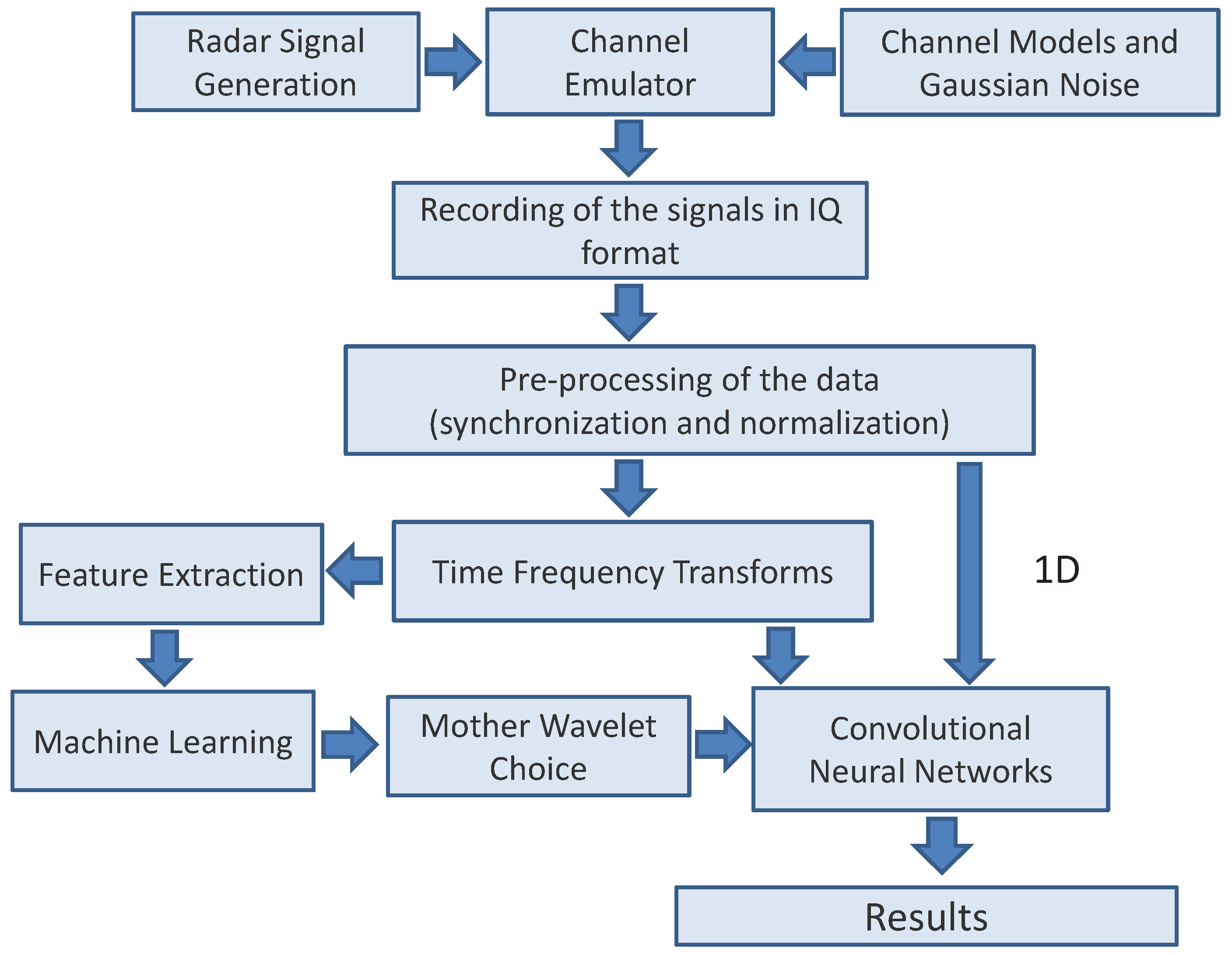
The overall methodology for the generation, processing and input to CNN is provided in
Figure 1. In the first phase, a weather radar pulse signal is generated with a signal generator in the JRC radio frequency laboratories as described in
Section 4. Then, the signals are transmitted through the channel emulator with different conditions of fading. The output of the channel emulator is recorded in IQ format and the data set is labeled: all the data related to a specific channel condition is labeled as such. Then channel conditions are based on the 3GPP-TDL models (3GPP-like channel models) defined in the standard 3GPP TR 38.901 version 14.0.0 Release 14 standard (page 66 to 70) [
20]. Additional details on the adopted 3GPP-like channel models are provided in
Section 4.2.
Six classes of labels are defined: No Fading, TDL-A, TDL-B, TDL-C, TDL-D, and TDL-E. The fading conditions are also generated in the channel emulator with different values of SNR in dB to evaluate the robustness of the proposed approach to the presence of noise. The data is then normalized on the basis of the RMS power. Then, different TFTs are applied to the signals. In this study, we have used the WAVELAB library from [
21] for the implementation of CWT. In the WAVELAB library, the mother wavelets are real. Then, the output of the application of the CWT is also real as the original raw data is real. The output of the TFTs is normalized between 0 and 1 to be given as an input to the CNN. The architecture of the CNN and related hyper-parameters is described in detail in
Section 5. Finally, the output of the CNN is used to evaluate the performance of each TFT using accuracy and confusion matrices. The main hyper-parameter of this approach is the mother wavelet to be chosen. In this study, we use the Gaussian, derivative Gaussian, Morlet, and Sombrero (i.e., Mexican hat wavelet), which are identified in the rest of this paper with the following notations: CWT-S (Sombrero), CWT-D (derivative Gaussian), CWT-G (Gaussian), and CWT-M (Morlet). The problem is still to find the optimal mother wavelet. A method based on the application of the CWT and the CNN classification for each mother wavelet would be cumbersome because the CNN classification takes a considerable amount of computing time and resources, and it should be preferably minimized. Then, a preliminary process is adopted to choose the optimal mother wavelet. The step of applying the CWT with four mother wavelets is still executed, but instead of giving the wavelet representations directly to the CNN, a feature extraction process is implemented where the entire CWT transformed sample (i.e., the weather radar signal) is represented with a significant dimensionality reduction with only three features: its variance, skewness, and kurtosis. These features have been chosen because they are commonly used in literature for feature extraction in wireless communication classification problems [
22], and they are simple to compute. Then, a shallow machine learning algorithm is applied for each of the mother wavelets. The mother wavelet, where the classification performance is the best, is chosen for the application of CNN. This adaptive approach is based on the assumption that the extracted features and the machine learning algorithms are able to select the optimal discriminating mother wavelet. This assumption has to be validated by the results of the data set. The advantage of the proposed approach is to save the repeated execution of the CNN with different mother wavelet representations at the cost of performing the feature extraction process and the application of the ML algorithms. Both steps require limited computing resources in comparison to the application of CNN, as shown in
Section 7.
Finally, another aspect of the proposed approach is related to the addition of Gaussian noise and the composition of the data set described in
Section 4.2. Two methods are applied in this study:
The training and test portions of the data set are selected from the data with the same level of SNR in dB.
The training portion of the data set is selected from the data at the highest level of SNR in dB considered in this study, while the test portion of the data set is selected from data at different levels of SNR in dB.
The first method (called SAMESNR in the rest of this paper) is simpler to execute because training and test are extracted from the same data set, and it is also more controlled, but it is not very realistic as the training is usually performed at high values of SNR while the conditions in the field can vary. The second method (called DIFFSNR in the rest of this paper) is more related to a practical application of the proposed approach. Both methods are used in this paper. In particular, the first method is used for the selection and identification of the hyper-parameters apart from the mother wavelet, which is evaluated in both methods. Additional details on the two methods, SAMESNR and DIFFSNR, are provided in
Section 7.
4. Test Bed and Materials
4.1. Test Bed
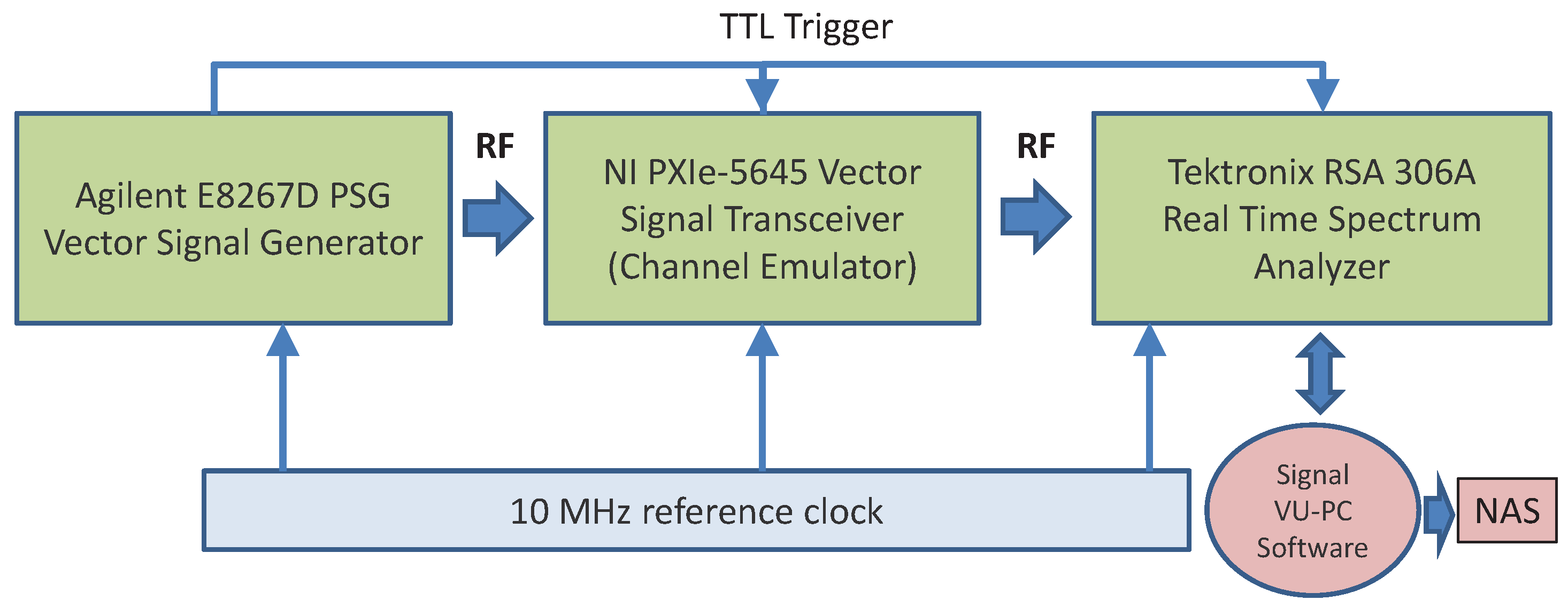
The test bed for the generation of the signals used in our analysis is described in
Figure 2. This is a conducted test bed connected with RF cables. The entire set-up was properly calibrated, and the loss of the RF equipment (e.g., RF cables and adapters) was recorded and considered in the measurement and data collection phases. The testbed is composed of the following laboratory equipment:
Agilent E8267D PSG Vector Signal Generator. This signal generator was used for a weather radar test signal defined in [
23] with a sampling frequency of 40.00 MHz and a pulse width of 1 microsecond. According to the technical specifications of [
23], such weather signal is repeated in time with two different Pulse Repetitions Frequencies (PRF)s. The first PRF (called PRF1 in the rest of this paper) is set to a value of 800 Hz, and the second PRF (called PRF2 in the rest of this paper) is set to a value of 1200 Hz. The number of pulses for each PRF is 18. This configuration with PRF1 and PRF2 creates a sequence of pulses with one pulse lasting 1 microsecond, one pause lasting 1.25 ms, one pulse lasting 1 microsecond, and one pause lasting 0.833 ms. The carrier frequency for the train of radar pulses is set to 5650 MHz in the PSG Vector Signal Generator.
The RF channel emulator based on the NI-VST (Vector Signal Transceiver by National Instruments) PXIe-5645R, which was extended with additional fading models (e.g., Nakagami-m). The channel emulator implements the TDL model as a modification (i.e., using the Nakagami-m fading model and with the first 6 taps) of the TDL fading models based on the standard 3GPP TR 38.901 Release 14 standard (version 14.0.0, page 66 to 70) [
20]. The Nakagami-m distribution was used because it has various advantages versus other fading models [
24]: (a) it has greater flexibility and accuracy in matching some experimental data than the Rayleigh, lognormal, or Rice distributions, (b) it is a generalized distribution, which can model different fading environments, and (c) Rayleigh and one-sided Gaussian distribution are special cases of Nakagami-m model.
Tektronix RSA 306A Real-Time Spectrum Analyzer with 40 MHz of bandwidth with SignalVU PC software, which is used to collect the signal output from the RF channel emulator. A sampling frequency of 28 MHz is used as an optimal balance between the need to properly sample the signals and to limit the amount of data to be processed by TFT algorithms and the CNN.
The digital output from the Real-Time Spectrum Analyzer was collected and recorded in a Personal Computer (PC) equipped with SignalVu-PC Software for further data processing using MATLAB. The description of the computing environment is in
Section 4.3.
4.2. Materials
As described in the previous section, the channel emulator implements 5 different TDL models, which are inspired by the TDL models defined in [
20] for 3GPP but which have been modified using the Nagakami-m fading model rather than Rayleigh or Rice model as in the initial definition of [
20] (i.e., 3GPP-like models). With the addition of the No Fading case, 6 different classes of wireless signals are used for channel identification. They are called in the subsequent parts of this paper (1) No fading, (2) TDL-A, (3) TDL-B, (4) TDL-C, (5) TDL-D, and (6) TLD-E.
To support a generalization of the results, the signals were processed with different values of m in the Nagakami-m fading model for each TDL class. The values of m = 0.5, 1, 2, 3, 4 were used.
A set of 1680 weather radar signals were generated for each value of m and for each of the 6 classes (e.g., an equal number of radar pulses was generated for the No fading case for consistency) for a total of 1680 × 5 × 6 = 50,400 signals samples on which the TFTs and the CNN algorithm was applied.
In addition, we evaluated the impact of different SNR levels expressed in dB, as previously mentioned. Starting from the baseline data set at SNR = 30 dB, different data sets were created with decreasing values of SNR in dB: −15 dB, −10 dB, −5 dB, 0 dB, 5 dB, 10 dB, 15 dB, 20 dB, and 25 dB. This range of values was chosen to evaluate the impact of noise with a good level of granularity (5 dB steps) and on the basis of the empirical observation that at −15 dB, every algorithm proposed in this paper reaches almost random choice classification, and it is pointless to evaluate even lower levels of SNR in dB. In the rest of this paper, this data set is called the weather radar data set.
Due to the similarity of the TDL fading models, the classification of this data set is particularly challenging (on purpose) as we do not limit the scope of the study to LOS/NLOS binary classification, but the objective is to distinguish different fading models as well.
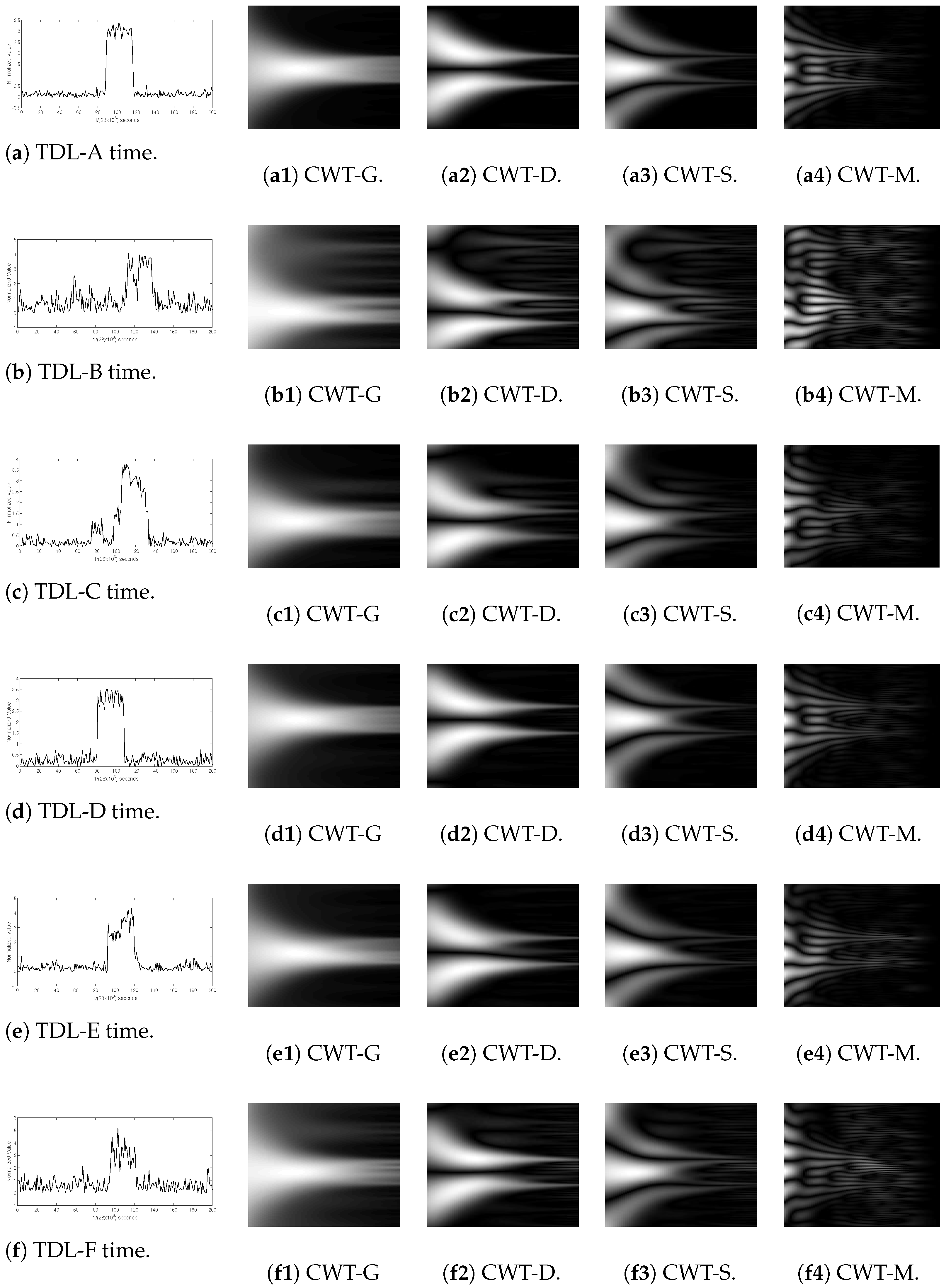
The visualization of one sample of each of the 6 different fading conditions and the related CWT transform is shown in
Figure 3, where it can be seen that some representations are similar (e.g., TDL-E, TDL-F) from a visual point of view (this will also be assessed in the
Section 7).
4.3. Computing Environment
The computing environment was based on MATLAB with the Deep Learning toolbox, the Signal processing toolbox for the spectrogram and Wigner-Ville distribution from Mathworks (MATLAB v2021a), the WAVELAB library from [
21] for the implementation of CWT. The computing platform used in this study was a desktop HP Z8 G4 with Intel Processor Xeon Silver 4214Y at 2.2 GHz, 40 GBytes of RAM, and one NVIDIA Quadro RTX 4000 as CUDA-enabled graphic card to support the Deep Learning algorithm.
5. Convolutional Neural Network Architecture
This section describes the CNN architecture and the metrics used to evaluate the performance of the different approaches, both SAMESNR and DIFFSNR.
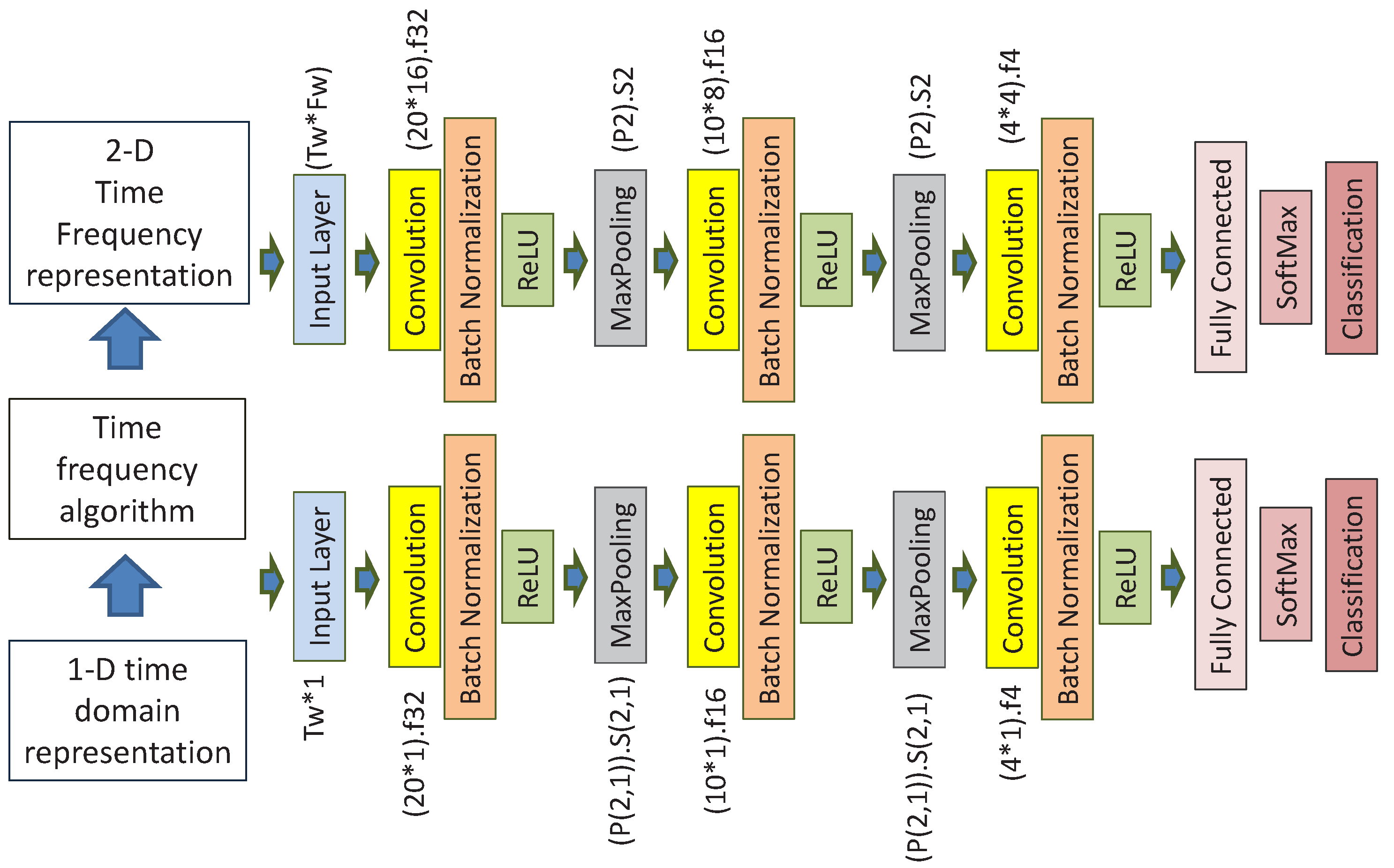
The architectures for the CNN implementation for the time–frequency input and the 1D time domain input are shown in
Figure 4. An architecture with 3 convolutional layers was identified to be the optimal architecture across the time–frequency representations and 1D representation as discussed in
Section 7. The 1D time-domain representation was also directly used as an input to a 1D CNN for comparison with the TFTs approach. Then, different TFTs were applied to the 1D time-domain representation to produce 2D representations (i.e., grayscale images), which are fed to the CNN. While the adopted CNN architecture is canonical, there are different hyper-parameters (e.g., solver algorithm) whose impact has been evaluated on the classification performance measured in terms of accuracy (see the end of this section for the definition of the evaluation metrics). The number of epochs was set to 40.
The most common hyper-parameters of each layer were optimized for each time–frequency transform and the 1D time domain representation. While this task seems to be cumbersome, the list of optimized hyper-parameters was limited to the list shown in
Table 1, where the range is shown for each hyper-parameter. The range of values is usually defined for the first layer and the subsequent layers are based on the value of the first layer. The optimal identified values are an example for a specific TFT the CWT with Sombrero mother wavelet. A similar process was performed for all the other TFTs and for the 1D time domain representation, but they are not shown here for reasons of space. The metric for the identification of the optimal values was accuracy. The values represented in
Figure 4 are an example of the optimal values for the optimization of the CWT (Sombrero wavelet) for the weather radar data set.
The entire weather radar data set was divided in 4 portions using a 4-fold approach where the testing portion was 1/4 of the entire data set, and the training set was 3/4 of the entire data set. Then, the ratio between the sizes of the testing and training data was 1/3. The training data set was further divided, with 10% of it allocated for the validation task. As it is a 4-fold algorithm, the training and data set portions were randomly selected from the main data set. To further improve the generalization of the results, the overall 4-fold classification process was repeated 10 times (then 4 folds per 10 = 40 times), and the results (i.e., accuracy) were averaged.
The results of the evaluation of the impact of the hyper-parameters listed in
Table 1 are shown more in detail in
Section 7 for a specific time–frequency representation (CWT with Sombrero mother wavelet). Other hyper-parameters have been also evaluated, but their impact was not shown in the paper because the differences were minimal. For example, the authors evaluated the performance of the hyper-parameter number of filters in the first convolutional layer using a range from 16 to 64 in step 16, and the value of 32 was finally used. The values of the hyper-parameters of the second and third convolutional layer (CL) were chosen on the basis of the values of the first. The number of filters in the second CL was half of the first, and the number of filters in the third CL was a quarter of the second.
The metrics used to evaluate the performance of the proposed approach are classification accuracy and confusion matrices. The accuracy is defined as:
In the equation, TP represents the number of True Positives, TN represents the number of True Negatives, FP represents the number of False Positives, and FN represents the number of False Negatives. In addition to the accuracy metric (which does not provide the values of FN and FP), we also use confusion matrices to evaluate the performance of the proposed approach. We use the notation of the confusion matrices where the rows of the matrix represent the instances of a true class while the columns represent the instances of the predicted class.
6. Time Frequency Transforms
The aim of this section is to describe the different TFTs used to convert the digitized signal output from the channel emulator into images, which are then given as input to the CNN.
Various TFTs and TFDs have been adopted in this study. Their selection is based on their rare use in literature for channel identification and, more generally, for wireless communication problems (e.g., radio frequency fingerprinting).
6.1. Spectrogram
The spectrogram is the squared magnitude of the continuous-time Short Time-Frequency Transform (STFT), which can be defined in the following equation for a signal x(t):
where
is a window function (the Hahn function was used in this study). Considering that function of STFT is the function of Fourier transform multiple by the window function, the STFT can be also called windowed Fourier transform or time-dependent Fourier transform. The size of the window is a hyper-parameter in the definition of the spectrogram.
The spectrogram has been used in this study because it was already adopted in the related literature in [
15] and it also commonly used together with CNN in other wireless communication problems such as RF fingerprinting in [
18,
25].
6.2. Continuous Wavelet Transform
The continuous wavelet transform (CWT) uses inner products to measure the similarity between a signal (i.e., the radar signal in a fading channel) and an analyzing function (i.e., a specific wavelet, also called a mother wavelet). The CWT compares the signal to shifted and compressed or stretched versions of a wavelet. The stretching operation is called dilation, while the scaling operation is referred to the physical notion of scale. The result of the CWT is obtained by comparing the signal to the wavelet at various scales and positions. If the wavelet is complex-valued, the CWT is a complex-valued function of scale and position. If the signal is real-valued, the CWT is a real-valued function of scale and position.
In this study, we used the CWT MATLAB implementation from the WAVELAB library [
21], and we used the pre-defined mother wavelets in the library: Sombrero, Derivative Gaussian, Gaussian, and Morlet. Each of the mother wavelets used in this study is defined in the following equations:
The CWT is used in this study because it was adopted in [
12] for LOS/NLOS channel identification to improve indoor positioning, and it has demonstrated superior performance to other time–frequency representation in other wireless communication problems in [
18].
6.3. Wiegner-Ville Distribution
The Wigner-Ville Distribution (WVD) function has been chosen in this study because it provides the highest possible temporal vs frequency resolution, which is mathematically possible within the limitations of the uncertainty principle. This characteristic is useful in the application of CNN because the high resolution can be exploited by the neural network to extract the discriminating elements of the fading channels. The downside of the WVD is the introduction of large cross terms between every pair of signal components and between positive and negative frequencies, which may confuse the CNN, especially in the presence of noise [
26]. There are different formulations in the literature of the WVD. In this paper, we adopt the following definition for a continuous signal x(t):
A smoothed version of the WVD (SWVD) is also used in this study, where independent windows are introduced to smooth in time and frequency:
The smoothed version SWVD was chosen because it may be more robust to the presence of noise. The word ’may’ is used because the smoothing effect could also obfuscate the same fading channel discriminating characteristics this study tries to classify. In literature, the WVD and SWVD were not used to the knowledge of the authors together with CNN for channel identification, but it was used to automatically recognize the waveform types of wireless signals in coexistence radar-communication systems in [
27], which prompted the authors of this study to investigate the application of WVD and SWVD to the channel identification as well.
6.4. Time Frequency Hyper-Parameters Optimization
The definition of the TFTs does also include parameters, which may have an impact on the classification performance. For each data set, an estimate of the optimal values of the parameters was performed, and the results are presented here.
7. Results
The aim of this section is to provide the results of the application of CNN. As described before, the application of the CNN in the presence of noisy samples can be executed using different approaches. In one approach (SAMESNR), the training and test phase is executed on subsets of the data set with the same level of SNR. In another approach (DIFFSNR), the training set is based on a subset of a data set at one or more specific levels of SNR in dB, and the testing and prediction are based on different levels of SNR in dB. The first approach is simpler to implement, and it is based on a coherent data set because the training and testing samples are extracted from the same data set. On the other hand, it is not consistent with a practical application of the fading channel classification because the SNR values of the data set on which the DL model is trained can be different from the actual SNR value in the field. The second approach addresses this shortcoming, but the different levels of SNR for the training and testing sets must be defined.
In this study, for the second approach, we set 30 dB for the SNR of the training data set and progressed lower values of SNR for the testing set. This execution aimed to reproduce a context where the training samples were collected in a relatively high SNR level in a laboratory, and then the fading channel prediction was actually performed in the field with more difficult propagation conditions and a strong presence of noise.
The first
Section 7.1 provides the results of the optimization process for the CNN, where the impact of the different hyper-parameters is evaluated and optimized using the SAMESNR method. The second
Section 7.2 provides the comparison of the results of the different approaches (e.g., 1D against time–frequency representations) for the SAMESNR method in terms of the evaluation metrics identified before (accuracy and confusion matrices). The third
Section 7.3 provides the comparison of the results of the different approaches (e.g., 1D against time–frequency representations) for the DIFFSNR method in terms of the evaluation metrics identified before (accuracy and confusion matrices).
A more important aspect presented in
Section 7.3 is related to the evaluation of the novel adaptive approach proposed in this paper. We have evaluated the adaptive approach for the DIFFSNR methods rather than the SAMESNR method because the differences in performances among the different combinations of the time–frequency transforms and CNN are more evident in the DIFFSNR method.
Finally, the fourth
Section 7.4 provides computing time estimates to execute the different steps in the proposed approach and highlights the considerable improvement in time efficiency in comparison to the traditional exhaustive approach.
Regarding the notation, the approaches based on the different time–frequency representations will be identified for the CWT with CNN as CWT-S, CWT-D, CWT-G, or CWT-M. For the application of CNN to the Wigner Ville distribution, the notation is WVD. For the application of CNN to the Smoothed Wigner Ville distribution, the notation is SWVD or Smoothed WVD. For the application of CNN directly to the 1D time domain representation of the signal, the notation is 1D.
7.1. Optimization of the Convolutional Neural Network Parameters with Training and Testing Data Set at the Same SNR Level
As anticipated in
Section 5, an assessment of the impact on the classification performance of specific CNN hyper-parameters was implemented, and the optimal values are shown in
Table 1 for a specific time–frequency representation: the CWT with the Morlet mother wavelet. The aim of this section is to show how significant can be the improvement in classification accuracy due to the optimal choice of the hyper-parameter value. Note that these results are also based on the optimal values of the voices per octave shown in
Table 2.
The results of the optimization process are shown in
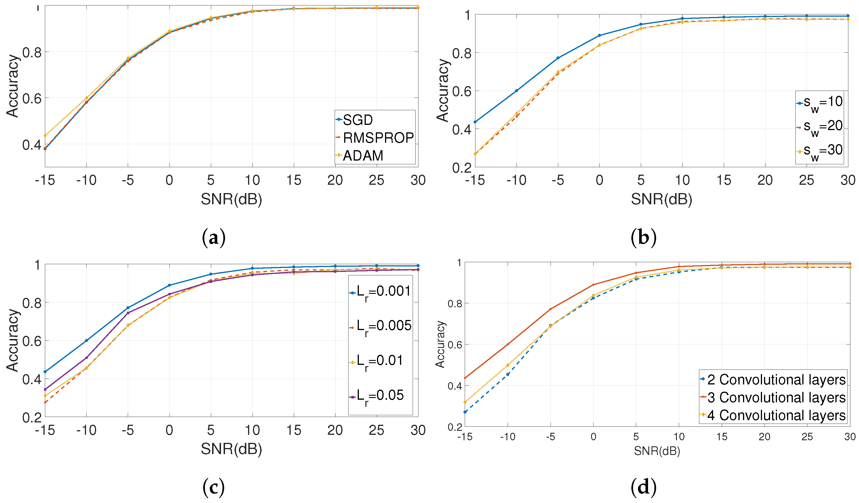
Figure 5 for the specific case of CWT-S for the weather radar data set.
Figure 5a shows the accuracy trend for different values of SNR in dB. It can be seen that the use of the Adam solver algorithm has a similar performance to the RMSProp and the SGDM, but it is slightly more robust for lower values of SNR in dB.
Figure 5b shows the accuracy trend for different values of the window size used in the first Convolutional Layer. It can be seen that a value of
equal to 10 provides the optimal accuracy at any value of SNR. A potential reason for this is that such a relatively small window supports a more effective extraction of the discriminating feature by the CNN algorithm. On the other hand, even smaller values of the window size may increase the computing time of the CNN.
Figure 5c shows the accuracy trends for different values of the initial learning rate used for training, where it can be seen that a value of 0.001 provides the optimal accuracy trend, in particular for its robustness to noise. As in the previous case, a smaller value of the initial learning rate may increase the computing time of the CNN.
Figure 5d shows the accuracy trends for the different numbers of convolutional layers used in the CNN architecture. It can be seen that three convolutional layers are optimal both at low values of SNR and at higher values of SNR. In fact, it is not necessary to increase the number of convolutional layers because four convolutional layers perform less than three convolutional layers.
7.2. Training and Testing Data Sets at the Same Level of SNR
This section aims to describe the result of the comparison of the approach DIFFSNR based on the different TFTs and the one-dimensional representation in the time domain for the data set used in this study.
The comparison of the approaches based on the different TFTs are presented in
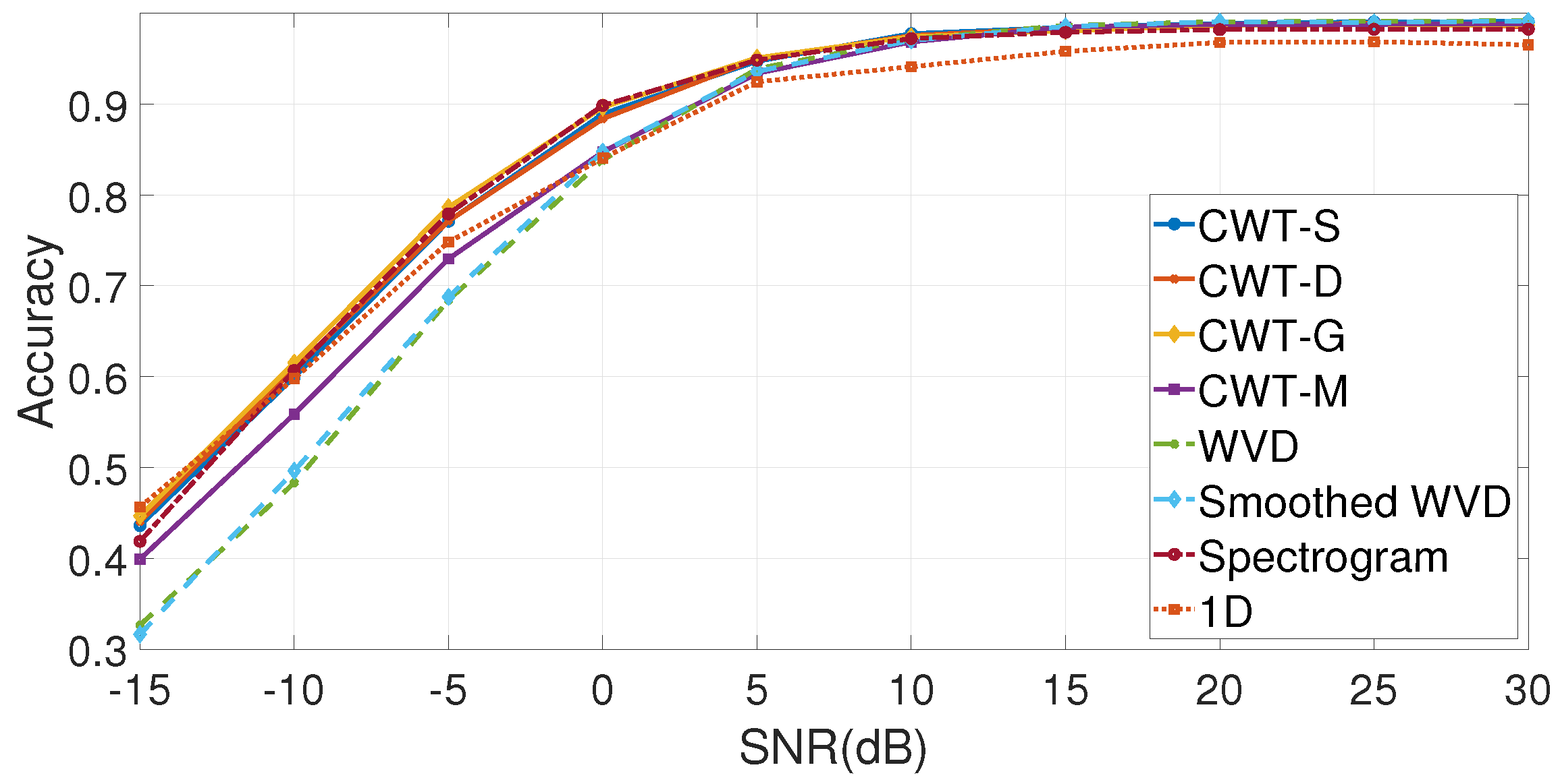
Figure 6 for different values of SNR in dB for the weather radar data set. The accuracy trend for the baseline application of CNN to the 1D time domain representation is also presented in
Figure 6. An initial result is that the combination of TFT with CNN has a significantly better performance than the application of CNN directly on the initial 1D time domain representation, in particular for values of SNR
dB. An additional result is that CWT usually performs better than other TFT in the presence of noise (values of SNR
dB). In particular, CWT is more robust than WVD and the Smoothed WVD in the presence of noise, even if the Smoothed WVD presents a very minor improvement in comparison to WVD. In low noise conditions (SNR
dB), all the TFTs combined with CNN have a very high classification accuracy making this approach quite suitable for the identification of wireless propagation channels, at least with the use of pulse-like signals such as the weather radar signal used in this study. This result is consistent with the results in the literature, where pulse-like signals are generally used for channel identification.
A detailed report of the accuracy values obtained for the different TFTs and the 1D time domain approach is shown in
Table 3 for specific values of SNR in dB.
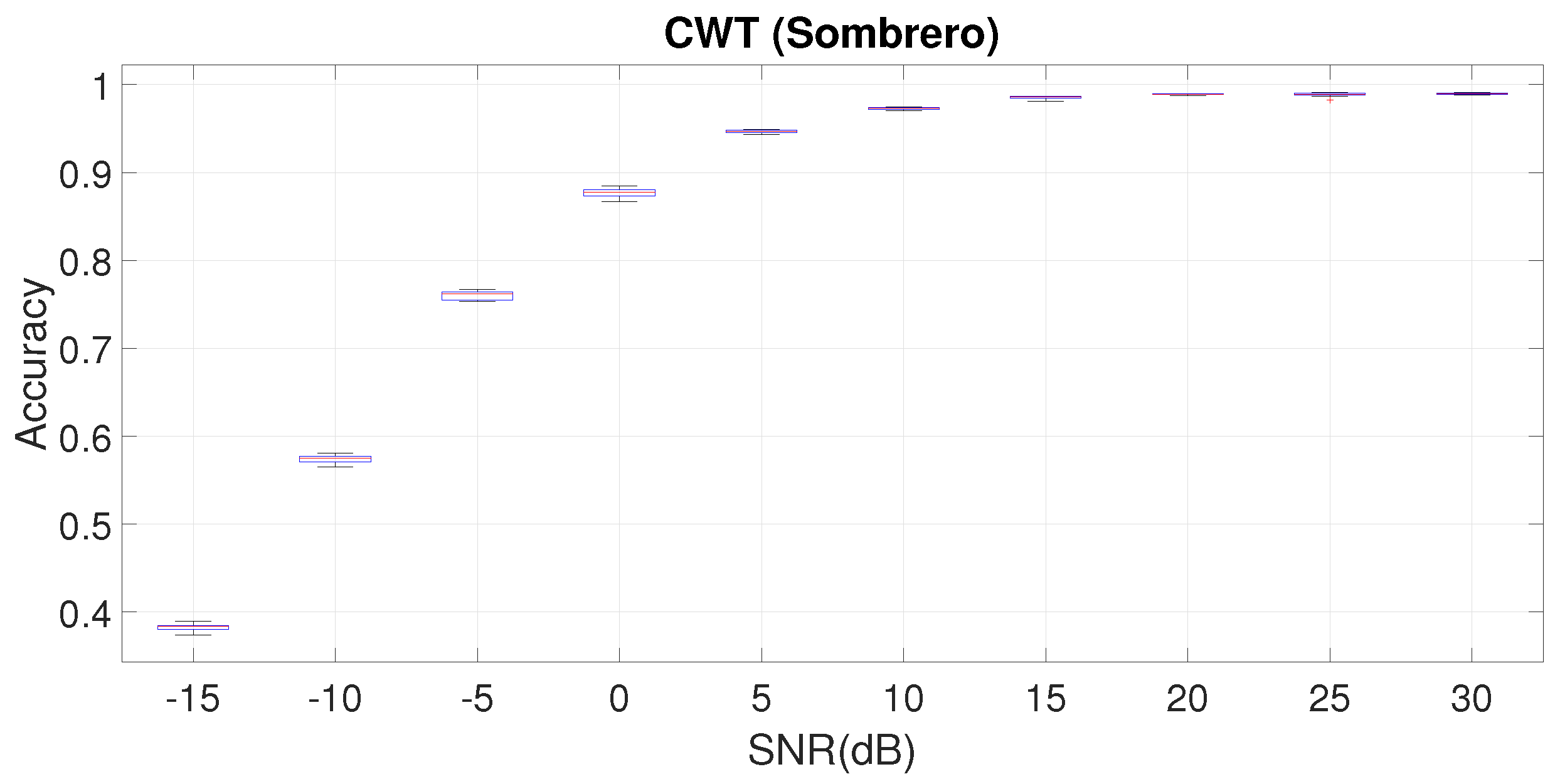
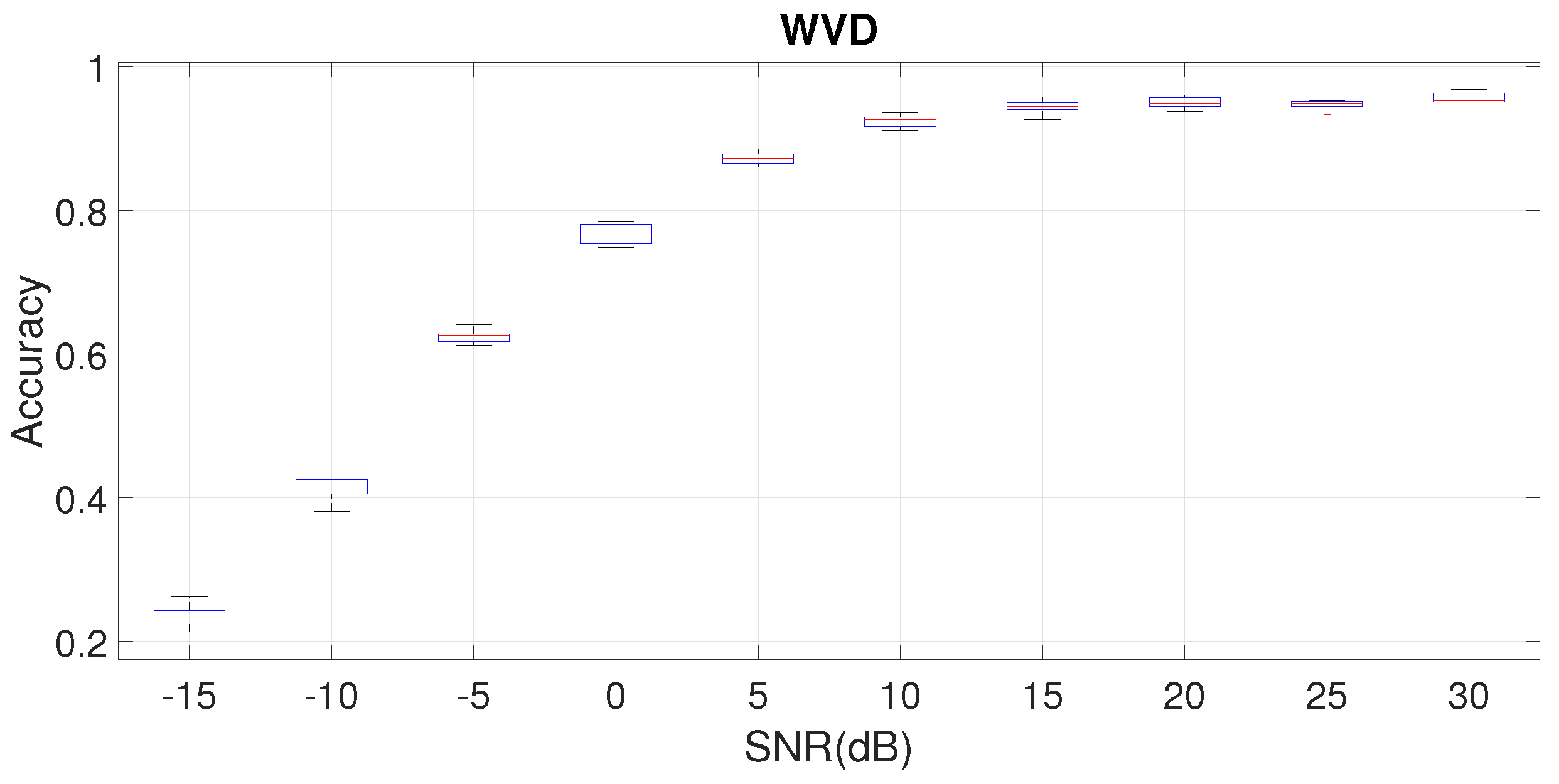
The results are also quite stable in terms of distribution of the accuracy values when we examine the results of the classification algorithm, which (as described in
Section 5) are repeated 10 times (the previous figures show the average of the accuracy results). Box plots are used to show the distributions of the results for the radar data set.
Figure 7 and
Figure 8 show the box plot, respectively, for the CWT (Sombrero) approach and the WVD approach. The distribution of the accuracy results is quite stable (minor spread of the values) in particular for the CWT (Sombrero) approach, while the accuracy results for the WVD approach are more spread out in particular for at lower values of SNR in dB SNR
dB.
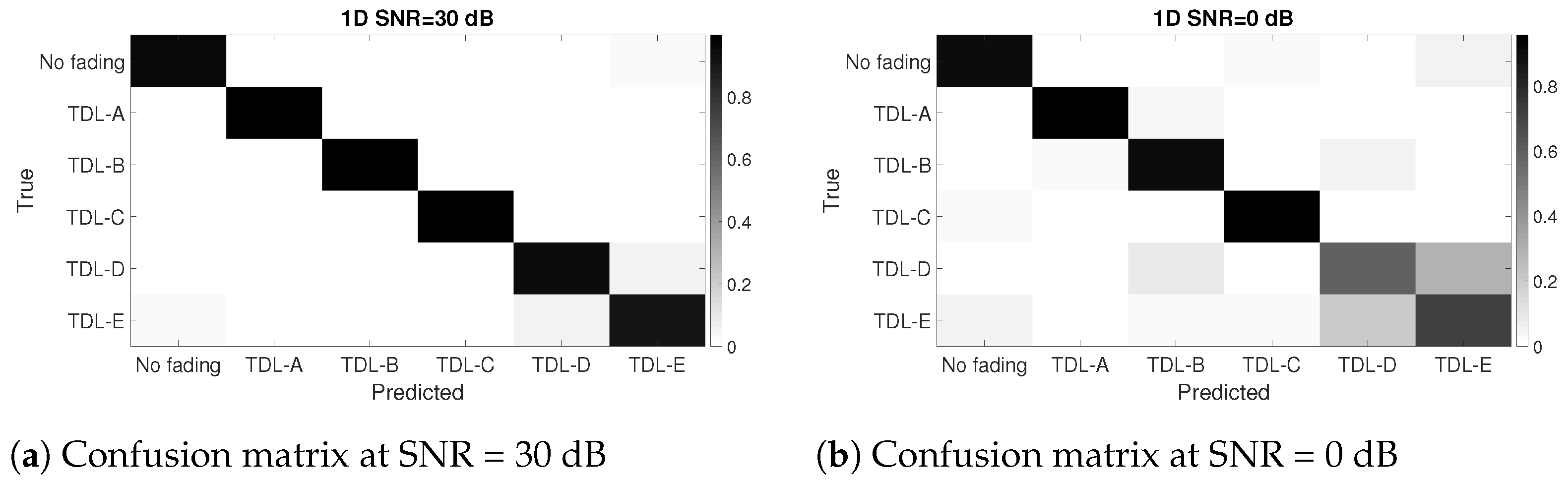
A more detailed view of the results of the channel identification is provided by the confusion matrices, which are shown in the following figures. In particular,
Figure 9 and the related sub-figures show the confusion matrices for SNR = 30 dB, and SNR = 0 dB for the CWT-S approach. Finally, a comparison with the 1D time domain is done by presenting the confusion matrices in
Figure 10 and related sub-figures for SNR = 30 dB and SNR = 0 dB.
The figures of the confusion matrices confirm the accuracy results shown in the previous figures: the CNN algorithm has some difficulties in identifying the different channel conditions in the strong presence of noise (e.g., low values of SNR). In particular, the TDL-D and TDL-E fading channels are quite difficult to distinguish even at SNR = 0 dB in all three representations, with the 1D and WVD representations providing the worst results (i.e., they are less distinguishable than CWT-S). This is consistent with the visual representations shown in
Figure 3, where it can be seen that the sample for TDL-D is quite similar to TDL-E with most of the CWT mother wavelets.
7.3. Training and Testing Data Sets at Different Levels of SNR and Results from the Adaptive Approach
The following
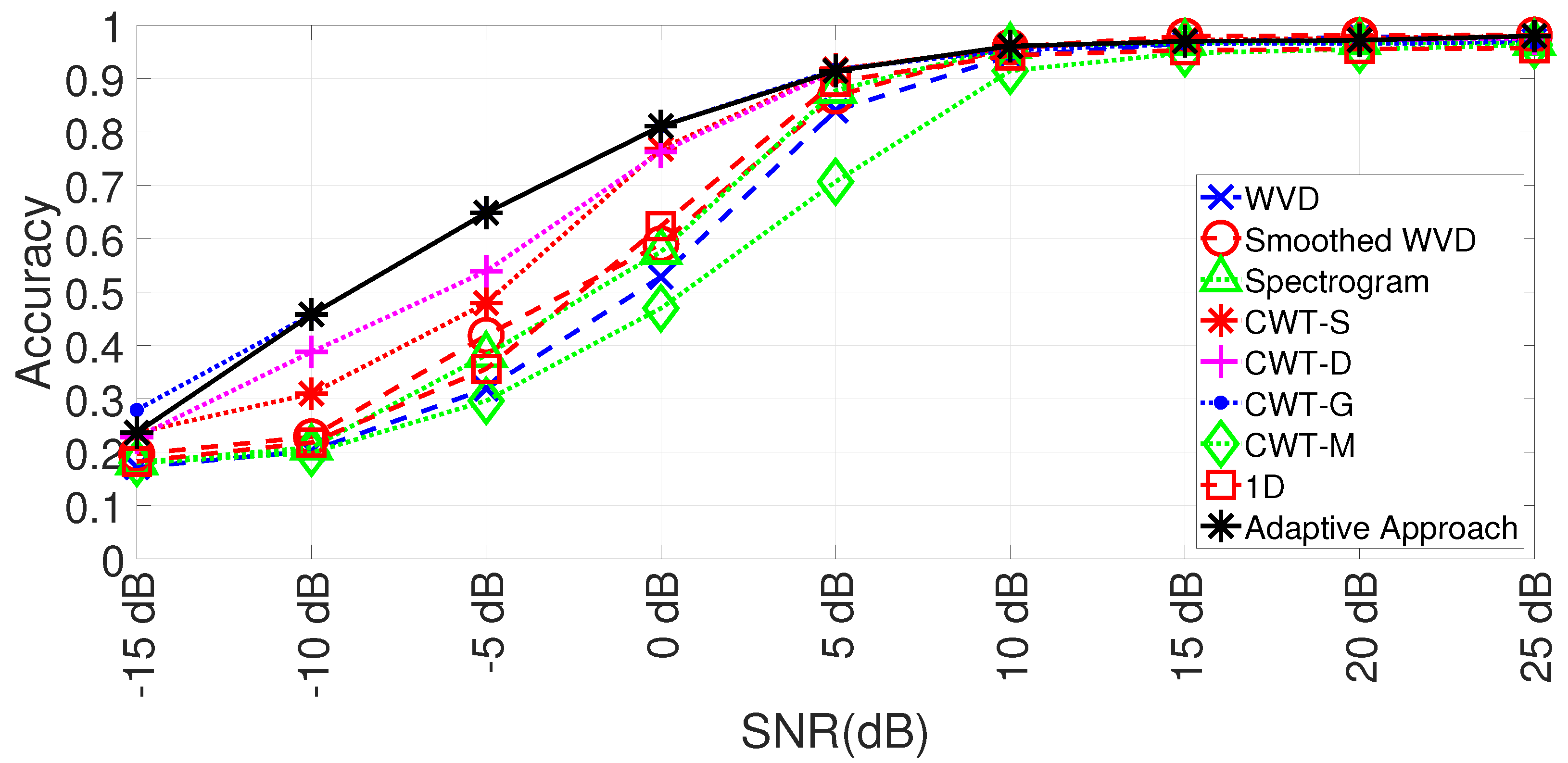
Figure 11 shows the comparison of the different techniques using the weather radar data set with the DIFFSNR method.
Figure 11 shows also the application of the adaptive proposed approach.
The first finding, which can be extracted from the analysis of
Figure 11, is that the act of training the CNN model with a data set at a different SNR than the testing data set usually degrades the classification performance in comparison to the SAMESNR method where the testing and training data sets are the same SNR level. This is to be expected because the presence of noise can change the structure of the data, and the CNN algorithm finds it more difficult to distinguish the fading classes. The second finding is that the choice of the Mother Wavelet (MW) is even more important in DIFFSNR than in SAMESNR because the differences between the different approaches are greater in DIFFSNR. We also note (in a similar way to the findings of SAMESNR) that no approach provides the optimal performance for all the values of SNR in dB. For example, the Smoothed WVD is more robust to noise than the WVD, as expected (because of the smoothing effect), but its accuracy is worst than WVD for values of SNR higher than 15 dB. A similar analysis is valid for the choice of the MW. Then, the application of an adaptive approach to automatically select the optimal wavelet is even more important in the DIFFSNR method than in the SAMESNR method.
Figure 11 shows the performance obtained for different values of SNR in dB for the adaptive method using the Decision Tree (DT) algorithm. It can be seen that the adaptive approach is able to select automatically the optimal or the quasi-optimal MW for each value of SNR in dB. The algorithm fails to find the optimal value in the presence of strong noise at SNR = −15 dB, presumably because the fading conditions are so obscured by the noise that the information on the optimal wavelet is basically lost. On the other hand, at SNR = 15 dB, no TFT combined with CNN is able to classify the fading channels correctly, and most of them achieve an accuracy, which is barely above the random choice (which is accuracy = 1/6 or 0.1(6)). The optimal performance is obtained with the CWT-G and secondly with CWT-S and CWT-D. This is also expected because these wavelets are the ones that are more similar to the original pulse-like weather radar signal. On the other hand, the impact of the fading channel conditions is able to distort such pulse-like signal, which is the reason why no approach is able to obtain the perfect classification accuracy of 100 even at SNR = 25 dB.
The adaptive curve shown in
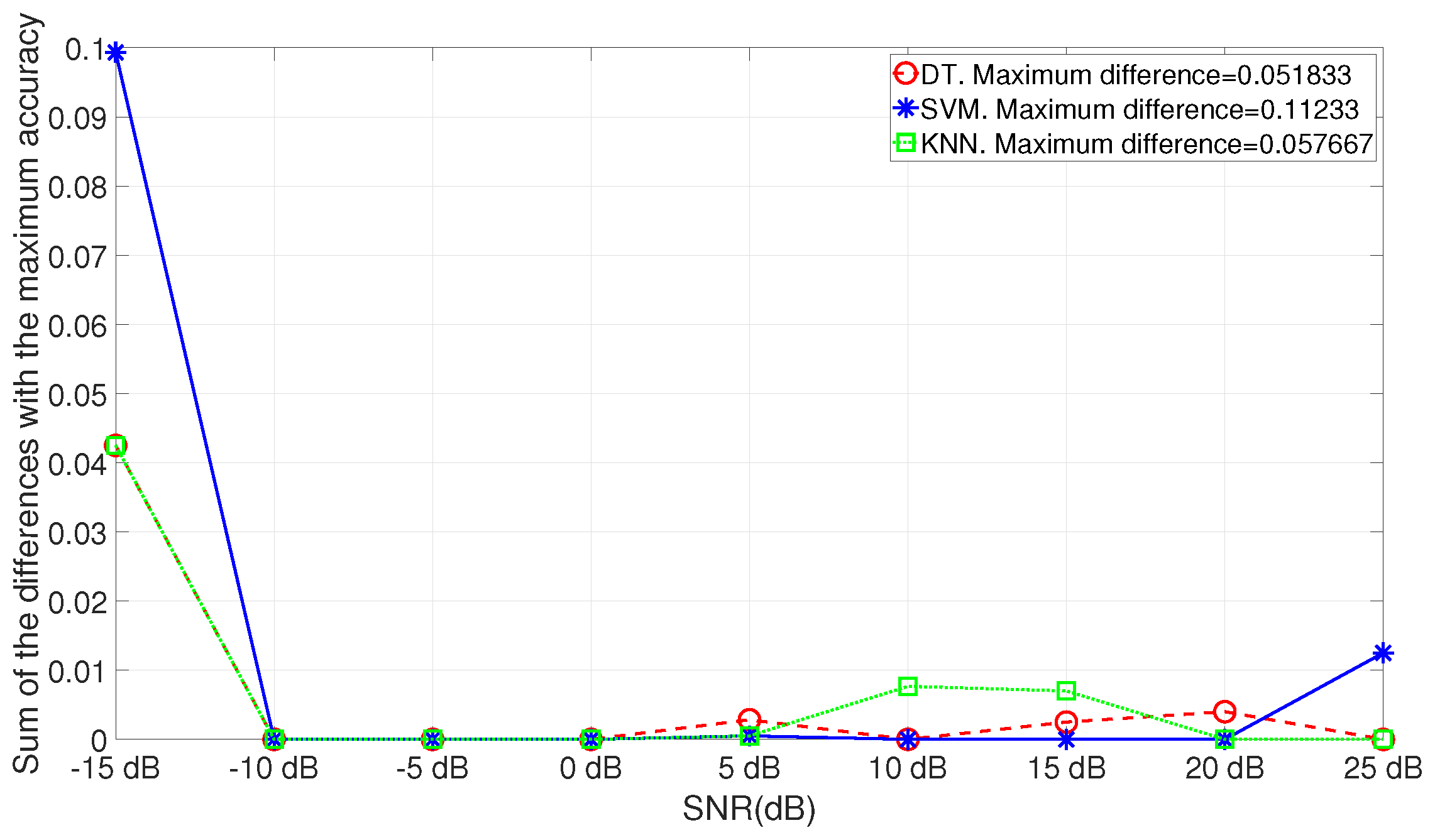
Figure 11 is obtained using the DT algorithm to choose the MWs. In this study, we have also used the SVM and KNN algorithms. Then, it is interesting to evaluate the related performance of the three algorithms. The results are shown in
Figure 12 where the differences between the ground truth (the optimal accuracy among all the approaches) and the value of the accuracy obtained for the MW obtained by the ML algorithm is shown for each value of SNR in dB and for all the three ML algorithms.
The overall sum of the differences across the 9 values of SNR in dB is shown in the legend box for each ML algorithm. We can see that the DT algorithm obtains the smaller sum of differences among the three ML algorithms, but the SVM is able to select the optimal MW for most of the values of SNR in dB. On the other hand, SVM is much worst than the other ML algorithms for the lowest value of SNR (SNR = −15 dB) and the highest value (SNR = 25 dB). Then, there is a potential trade-off to consider.
The following
Table 4 summarizes the numeric results obtained for the accuracy among the different approaches and shows the results of the selection of the ML algorithms among the mother wavelets.
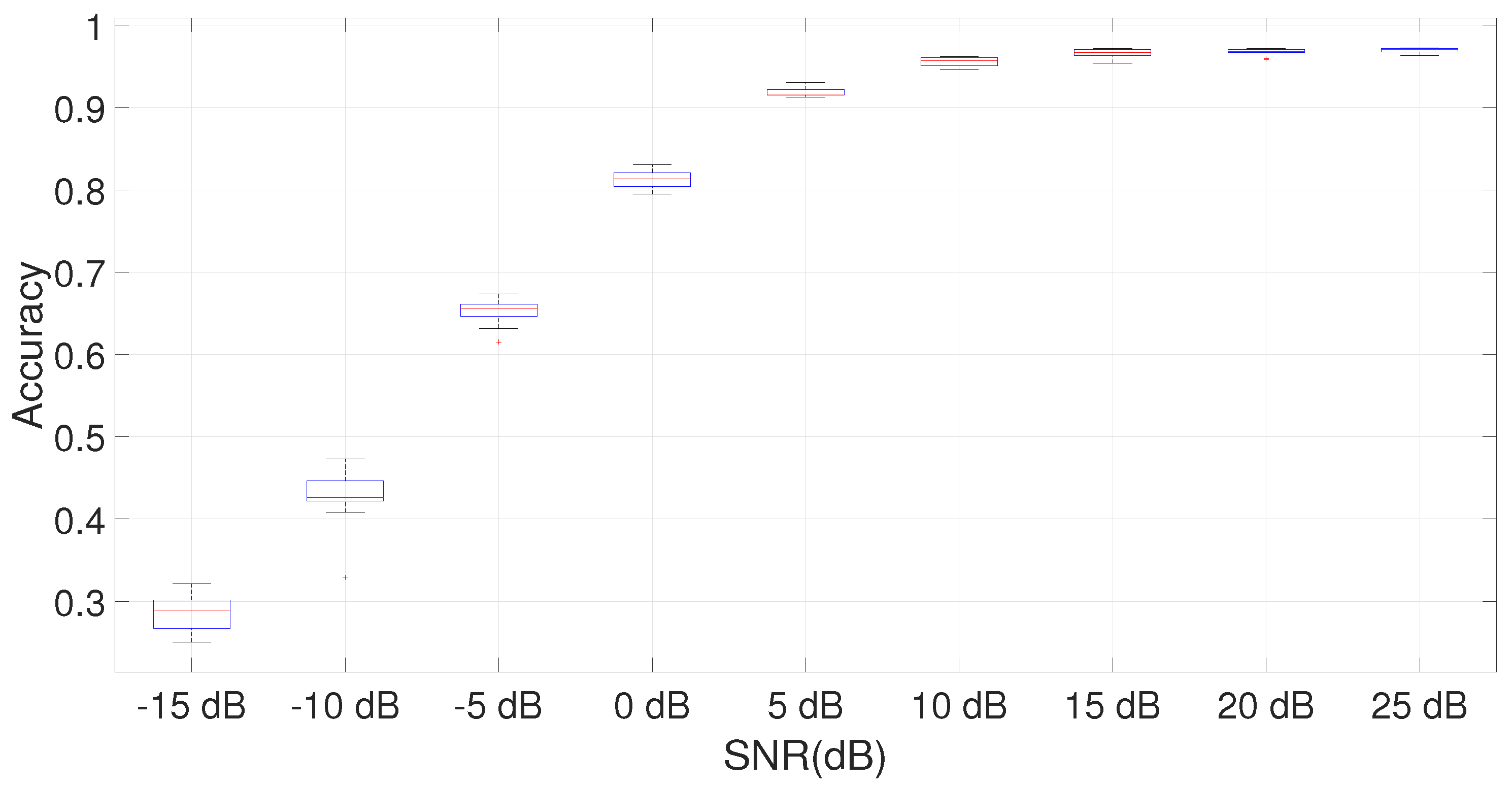
In a similar way to what was shown in the previous
Section 7.2, we also present the box plot of the accuracy for one time–frequency (CWT-G) with CNN. We choose this mother wavelet because it provides superior performance for DIFFSNR to the other MWs.
Figure 13 shows that the variability (i.e., the standard deviation of the distribution of the results) in the DIFFSNR method is slightly larger than in the SAMESNR method. This is also to be expected because the structure of the data can be quite different in the training data set taken at SNR = 30 dB and in the testing data sets at different values of SNR.
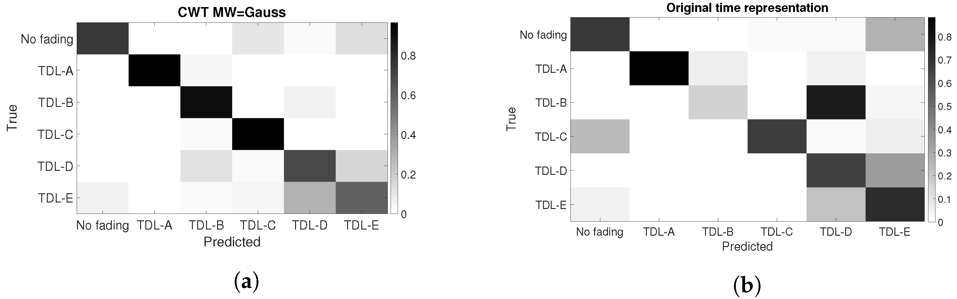
To complete the evaluation of the DIFFNSR method, we also show in this subsection similar results to what is shown in the previous
Section 7.2.
Figure 14a,b show the confusion matrices obtained using the CWT-G at SNR = 0 dB and the 1D or Original time representation. It can be seen that we obtained similar results for the DIFFSNR method as in the SAMESNR method. The TDL-D and TDL-E fading conditions are more difficult to distinguish. At the same SNR, the application of CNN with the original time representation is much worse than the combination of CWT MW = Gaussian and CNN because there is a relevant number of FP and FN for all the fading conditions.
7.4. Computing Time and Efficiency of the Adaptive Approach
We conclude the results sections with some consideration of the computing times needed to execute the steps of the proposed approach and the time efficiency of the adaptive approach. Without using the adaptive approach, an exhaustive optimization across the 4 selected MWs would require the execution of the CNN classification (model training and prediction) four times to identify the optimal accuracy.
Using the computing environment described in
Section 4.3, the calculated CNN model training time is 1165 s, and the prediction time is 4.11 s for CWT-G at SNR = 25 dB with the DIFFSNR method, and the other MWs have similar computation times as the size of the input data is the same across the MWs, and the CNN architecture is quite similar (the only differences are the values of some hyper-parameters). The adaptive approach requires the calculation of the three features (i.e., variance, skewness, and kurtosis) on the entire data set and the execution of the ’shallow’ machine learning algorithm. This time to calculate the three features and create the feature matrix is, on average, 20.6 s across the 4 different MWs. Taking as an example the DT algorithm, which provided the optimal performance across the different values of SNR (see
Figure 12), the time to generate the DT training model is 0.89 s, and the testing (prediction) is 0.024 s. Then, the overall computing time to implement the adaptive approach across the four considered MWs is 86.056 s, which is negligible (ratio of 0.01675) in comparison to the repetition of the CNN classification time for each MW. Then, the proposed approach is able to provide a significant gain in computing time.
8. Conclusions and Future Developments
This paper presented a study on the application of time–frequency transforms in combination with CNN for the problem of channel identification. The recognized performance (in the research literature) of CNN for the classification of images has been exploited by converting digitized radio frequency signals to images using TFTs. The results show that this approach is preferable in terms of identification accuracy than the application of CNN directly to the 1-dimensional representation of the signals as commonly done in literature at the cost of performing the specific TFT.
An extensive evaluation of the discriminating power of the different TFTs has been performed in this paper for a data set based on pulse-like weather radar signals in two different configurations. One configuration where the training and test portions of the data set have the same values of SNR in dB and another where the training and test portions of the data set have different values of SNR in dB. The results show that an accurate selection of the TFT is important to obtain an optimal classification in both configurations. In addition, there is a potential trade-off between high channel identification accuracy and robustness to noise. The application of CWT usually provides superior performance, especially in the presence of noise to the other time–frequency transform, but it presents the challenge of choosing the optimal mother wavelet. An exhaustive approach would require the repetition of the CNN classification for each mother wavelet, which will be demanding from the computing point of view. Then, this paper presented an adaptive algorithm to select the optimal mother wavelet based on the application of feature extraction algorithms and ’shallow’ machine learning, which has a minor impact on the overall computing time (less than 2% overhead in comparison to the CNN classification) but it supports the optimal or quasi-optimal selection of the mother wavelet at each level of SNR.
While the performance of time–frequency CNNs has been attempted in literature for other radio frequency classification problems such as radio frequency fingerprinting, such an extensive study for the problem of channel identification is novel to the best knowledge of the authors, especially with the application of the adaptive method.
Future developments will investigate other data sets to investigate the generalization of the approach proposed in this paper. In addition, other TFTs based on the synchrosqueezing concept will also be explored.


