Article

On the Semantics of Hybrid ASP Systems Based on Clingo

1
Department of Computer Science, University of Corunna, 15008 A Corunna, Spain
2
College of Information Science & Technology, University of Nebraska at Omaha, Omaha, NE 68182, USA
3
Department of Computer Science, University of Potsdam, 14469 Potsdam, Germany
*
Authors to whom correspondence should be addressed.
Algorithms 2023, 16(4), 185; https://doi.org/10.3390/a16040185
Submission received: 11 February 2023 / Revised: 17 March 2023 / Accepted: 22 March 2023 / Published: 28 March 2023
(This article belongs to the Special Issue Hybrid Answer Set Programming Systems and Applications)

Abstract

:
Over the last decades, the development of Answer Set Programming (ASP) has brought about an expressive modeling language powered by highly performant systems. At the same time, it gets more and more difficult to provide semantic underpinnings capturing the resulting constructs and inferences. This is even more severe when it comes to hybrid ASP languages and systems that are often needed to handle real-world applications. We address this challenge and introduce the concept of abstract and structured theories that allow us to formally elaborate upon their integration with ASP. We then use this concept to make the semantic characterization of clingo’s theory-reasoning framework precise. This provides us with a formal framework in which we can elaborate upon the formal properties of existing hybridizations of clingo, such as clingcon, clingo[dl], and clingo[lp].

1. Introduction

Answer Set Programming (ASP) is about mapping a logic program onto its so-called stable models. Over the decades, stable models have been characterized in various ways [1], somehow underpinning their appropriateness as semantics for logic programs. However, over the same period, the syntax of logic programs has continuously been enriched, equipping ASP with a highly attractive modeling language. This development also brought about much more intricate semantics, as nicely reflected by the long distance traveled from the mathematical apparatus used in the original definition [2] to the one for capturing the input language of the ASP system clingo [3].
With the growing range of ASP applications in academia and industry [4], we also witness the emergence of more and more hybrid ASP systems [5,6], similar to the rise of SMT solving from plain SAT solving [7]. From a general perspective, the resulting paradigm of ASP modulo theories (AMT) can be seen as a refinement of ASP, in which an external theory certifies some of a program’s stable models. A common approach, stemming from lazy theory solving [7], is to view a theory as an oracle that determines the truth of a designated set of (theory) atoms in the program. Meanwhile, this idea has been adapted to the setting of ASP in various ways, most prominently in Constraint ASP [5], extending ASP with linear equations over integers in various ways [8,9,10,11,12,13,14]. Beyond this, ASP systems such as clingo or dlvhex [15] leave the choice of the specific theory largely open. For instance, clingo merely requires fixing the interaction between theories and their theory atoms. As attractive as this generality may be from an implementation point of view, it complicates the development of generic semantics that are meaningful to existing systems. Not to mention that in ASP, the integration of theories takes place in a non-monotonic context.
As a matter of fact, most formal accounts of existing hybrid systems are implementation driven and lack a clear elaboration of the underlying semantic principles. We address this by separating the semantic foundations of hybrid languages from the corresponding systems’ design decisions. As a result, we present a framework in which we can characterize such decisions semantically. More precisely, we provide an extension of logic programs to incorporate very general abstract theories for which no predefined syntax is assumed. We extend the semantics of stable models for these programs, dealing with two types of theory atoms called defined and external. We further classify some types of abstract theories, which we call structured, where we may distinguish variables inside atoms, and the semantics can be defined in terms of denotations (via functions assigning values to those variables). Finally, we explain how several existing hybrid ASP systems, such as clingcon, clingo[dl], and clingo[lp], can be accommodated as instances of this general framework.

2. Background

We start considering an alphabet consisting of two disjoint sets, namely, a set A of propositional (regular) atoms and a set T of theory atoms, whose truth is governed by some external theory. Several theory atoms may represent the same theory entity. We use letters a , s , and b for atoms in A , T , and A T , respectively. In clingo, these theory atoms are expressions preceded by ‘&’, but their internal syntax is not predetermined: it can be defined by the user to build new extensions. As an example, the system clingcon extends the input language of clingo with linear equations, represented as theory atoms of the form
& sum { k 1 x 1 ; ; k n x n } k 0
where for each i such that 0 i n , each x i is an integer variable and each k i Z is an integer constant, whereas ≺ is a comparison symbol, such as <=, =, !=, <, >, >=. As we said above, we may have two different theory atoms, such as & sum { x } > 0 and & sum { x } > = 1 , actually representing the same condition (as a linear equation).
A literal is any atom b A T or its default negation ¬ b . A T -logic program over A , T is a set of rules of the form
b 0 b 1 , , b n , ¬ b n + 1 , , ¬ b m
where b i A T for 1 i m and b 0 A T { } with A T denoting the falsum constant. We let notations h ( r ) = def b 0 , B ( r ) + = def { b 1 , , b n } , and B ( r ) = def { b n + 1 , , b m } stand for the head, the positive, and the negative body atoms of a rule r of the form of (2). The set of body atoms of r is just B ( r ) = def B ( r ) + B ( r ) . Finally, the sets of body and head atoms of a program P are respectively defined as B ( P ) = def r P B ( r ) and H ( P ) = def { h ( r ) r P } { } , as expected. An example of a system using T -logic programs is the aforementioned clingcon, whose theory atoms correspond to linear integer equations. We refer to logic programs augmented by such theory atoms as clingcon-programs.
Next, we describe the semantics of T -logic programs in clingo [16], used for several extensions such as the addition of difference constraints in clingo[dl], of linear equations over integers in clingcon, and over reals in clingo[lp]. In all these systems, we can see the role of the corresponding external theory as a kind of “certification authority” that sanctions regular stable models whose theory atoms are in accord with their underlying constraints. To this end, we envisage a two-step process: (1) generate regular stable models and (2) select the ones passing the theory certification. In step (1), we ignore the distinction between atoms in A and T and plainly apply the stable model semantics [2]. More precisely, a set X A T of atoms is a model of a T -logic program P over A , T , if, for every rule r P such that B ( r ) + X and B ( r ) X = , we have h ( r ) X . In the case of an integrity constraint with h ( r ) = , note that does not belong to X A T . The stable models of P are defined via the reduct of P relative to a set X of atoms, viz.
P X = { h ( r ) B ( r ) + r P , B ( r ) X = } .
Then, as usual, a set, X, of atoms is a stable model of P if X is the least model of P X . In step (2), an external theory T is used to eliminate any stable model X whose theory atoms X T are not in accord with T . Suppose step (1) yields a stable model of a clingcon-program containing both atoms & sum { x ; 2 y } > 9 and & sum { 2 x ; 4 y } < = 6 . This stable model would not pass theory certification since no values for integer variables x and y can satisfy both corresponding linear equations, viz. x + 2 y > 9 and 2 x + 4 y 6 (note that the latter is equivalent to x + 2 y 3 ).
In fact, the treatment of each theory atom s (as obtained in the stable model) leaves room for different semantic options [16]. The first option is about the justification for the truth of s in step (1). A theory atom s is called defined if its truth must be derived through the program’s rules. Otherwise, s is said to be external, and we are always free to add it to the program without further justification. A second semantic option has to do with how we treat s X for a stable model X in step (2). We say that s is strict when s X implies that the theory check requires the “opposite” constraint of s to be satisfied. Otherwise, we say that s is non-strict, and the fact s X has no relevant effect during theory certification. Of course, in both cases, s X implies that the constraint of s is satisfied. As an example, suppose that s is the strict atom & sum { 2 x ; 4 y } < = 6 , and we get s X in some stable model X. Then, step (2) imposes the same constraint as if we had obtained atom & sum { 2 x ; 4 y } > 6 in X.
Janhunen et al. [14] argue that combinations (non-strict, defined) and (strict, external) are the only sensible ones for linear equation theories. With our focus on these theories, we follow this proposition, and partition the set T of theory atoms into two disjoint sets, E and F , standing for external and founded atoms, respectively. Intuitively, each external atom in E is interpreted as (strict, external), so its truth requires no justification, whereas if we decide to make it false, then its corresponding opposite constraint must be considered in step (2). On the other hand, founded atoms in F are those interpreted in a (non-strict, defined) manner, so they must be derived by the T -logic program, and when they remain eventually false, they do not impose any additional constraint on the final solution. Additionally, we require that founded atoms do not occur in the rule bodies, that is, B ( P ) F = , for any program P. We do allow external atoms to occur in the head, but, as we see later, they can always be equivalently shifted to the body. For the sake of brevity, we assume that an atom that only occurs in rule heads (but not in bodies) is founded unless explicitly stated otherwise. Let us emphasize that any atom that occurs in some body is mandatorily external, as discussed above. The signature of a program, P, as described above, is denoted as A , T , E , leaving F implicit.
With this restriction to two interpretations of theory atoms, we can formulate clingo’s semantics for T -logic programs as follows [16]: Informally speaking, a T -solution S is a subset S T of theory atoms whose associated constraints are “sanctioned” by abstract theory T ; this is made precise in Section 3. A set X A T of atoms is a T -stable model of a T -logic program P over A , T , E , if there is some T -solution S such that X is a stable model of the logic program
P { s s ( S E ) } { s s ( T H ( P ) ) S } .
That is, external atoms in S are added as facts to the program, whereas for any theory atom s occurring as a rule head but not in S, we add the constraint s . For illustration, consider the clingcon-program P ( 4 / 5 ) :
a & sum { x ; y } = 4
& sum { y ; z } = 2 a
This program contains two theory atoms: & sum { x ; y } = 4 and & sum { y ; z } = 2 . We refer to them by s 1 and s 2 , respectively. Theory atom s 1 is external since it occurs in the body of a rule, whereas we decide that s 2 is founded.
As explained above, the absence of any external atom, s T , in our candidate set, s S , imposes its complementary constraint to be satisfied. This is the so-called “strict” behavior. For this reason, we assume that, for any external atom, there always exists another external atom that is associated with that complementary constraint, even if this complementary atom does not occur in the program. We formalize this intuition in Section 3 below. In our example, since s 1 is external, we require a second, implicit external atom & sum { x ; y } ! = 4 , which we name s 3 , for short, and which stands for the complement of s 1 . As a result, our example deals with two external atoms E = { s 1 , s 3 } that are complementary to each other and one defined atom F = { s 2 } . Another consequence of the strict behavior is that any candidate T -solution S must contain either s 1 or s 3 , because the absence of one of them implies forcing the other, whereas the two of them cannot be selected at the same time because they are inconsistent altogether.
To obtain the stable models of P ( 4 / 5 ) , we must decide first which candidate set S of theory atoms are actually T -solutions. Although the definition of T -stable models starts by considering each T -solution S and builds an associated program (3) afterward, in practice, we can just start from any possible candidate set of theory atoms S to form program (3) and just check if they form a T -solution once we obtain the stable models X for that program. In our example, we are free to either add the external atom s 1 or its complement s 3 as a fact. If we decide to leave s 2 S , we must add the constraint s 2 . This amounts to two possibilities: X 1 = { s 1 , s 2 , a } and X 2 = { s 3 } . If T is the theory of linear equations, it is not difficult to see that S 1 = X 1 T = { s 1 , s 2 } is a T -solution because the associated constraints x + y = 4 and y + z = 2 are satisfiable: as a justification take, for instance, the variable assignment { x 2 , y 2 , z 0 } . When we use a variable assignment in this way, we say that it constitutes a witness of satisfiability for the set of constraints. In the case of S 2 = X 2 T = { s 3 } , we must simply satisfy the constraint x + y 4 and we can use, for instance, the witness { x 0 , y 0 , z n } with n being any integer (note that the value of z is irrelevant for satisfying this constraint).

3. Transformation-Based Semantics Revisited

Now, we provide a characterization of the theory reasoning framework of clingo that allows for formal elaborations of T -logic programs. To this end, we introduce the concept of an abstract theory T , which is our key instrument for establishing more fine-grained formal foundations. With it, we revisit the transformation-based approach and give a formal account of T -solutions.

3.1. Abstract Theories

An abstract theory T is a triple T , Sat , · where T is the set of theory atoms we can handle in the theory, Sat 2 T is the set of T -satisfiable sets of theory atoms, and · : T T is a function mapping theory atoms to their complement such that s = s for any s T . We define S = { s s S } for any set S T . Note that the set Sat acts as an oracle whose rationality is beyond our reach: to see if some set S of theory atoms is satisfiable, we may only check S Sat .
Despite the limited structure of such theories, some simple properties can be formulated: a set S T of theory atoms is
  • inconsistent, if both s S and s S for some atom s , (consistent otherwise)
  • Z -complete for some subset Z T , if for all s Z , either s S or s S , and
  • closed, if s S implies s S .
The definition of completeness is relative to some subset Z T of theory atoms, but when Z = T , we simply say that S is complete. An abstract theory T = T , Sat , · is consistent or complete if all its T -satisfiable sets S Sat are consistent or complete, respectively.
Note that any non-empty closed set S is inconsistent but can be T -satisfiable (e.g., for paraconsistent theories). We mostly use closed sets to describe subtypes of theory atoms rather than satisfiable solutions.
As an example, consider an abstract theory L = T , Sat , · of linear equations that can be used to capture clingconprograms, where
  • T is the set of all expressions of form (1),
  • Sat is the set of all subsets S T of expressions of form (1) for which there exists an assignment of integer values to their variables that satisfies all the linear equations in S with their usual meaning, and
  • the complement function is defined such as & sum { } c is & sum { } c with defined according to the following table:
<==!=<>>=
>!==>=<=<
Note that the set of theory atoms in L is closed.
Similarly, to cover clingo[dl]-programs, we introduce abstract theory D capturing difference constraints over integers, which is a subset of the already seen abstract theory L where theory atoms have the fixed form & sum { 1 x ; ( 1 ) y } < = k but are rewritten instead as:
& diff { x y } < = k
where x and y are integer variables and k Z .
Even though this definition of abstract theories is limited to a minimum set of requirements (no particular syntax, a set Sat used for satisfiability testing and a complement function), we can already define an abstract form of entailment as follows.
Definition 1 (Abstract Entailment).
Let T = T , Sat , · be an abstract theory. We say that a set S T of theory atoms entails a theory atom s T , written S | T s , when S { s } Sat .
In other words, S | T s when adding the complement of s to S becomes inconsistent. When S = { s } is a singleton, we normally remove the set braces and just write s | T s instead of { s } | T s . For example, it is easy to see that
& sum { x ; y } > = 1 | L & sum { x ; y } > = 0
because the pair of atoms & sum { x ; y } > = 1 and & sum { x ; y } < 0 (the complement of & sum { x ; y } > = 0 ) are in no satisfiable set in Sat under the usual meaning of linear equations.

3.2. Stable Models of Logic Programs with Abstract Theories

With a firm definition of what constitutes a theory T , we can now make precise the definition of a T -solution and T -stable model of a T -logic program given in (3). For clarity, we refine those definitions by further specifying the subset of external theory atoms in E . Moreover, given any set S of theory atoms, we define its (complemented) completion with respect to external atoms E , denoted by Comp E ( S ) , as the following superset of S:
Comp E ( S ) = def S ( E S )
In other words, we add the complement atom s for every external atom s that does not occur explicitly in S. Note that S is E -complete iff Comp E ( S ) = S . As an example, consider an abstract theory from L with the theory atoms T = { s 1 , s 2 , s 3 , s 4 } given above with
s 1 = ( & sum { x ; y } = 4 ) s 2 = ( & sum { y ; z } = 2 ) s 3 = ( & sum { x ; y } ! = 4 ) s 4 = ( & sum { y ; z } ! = 2 )
Suppose we only have one external atom E = { s 1 } and assume that the complements s 1 = s 3 and s 2 = s 4 are defined as expected. Then, set S = { s 2 } is E -incomplete because neither s 1 S nor s 1 = s 3 S . The completion of S corresponds to
Comp E ( S ) = S ( E S ) = { s 2 , s 1 } = { s 2 , s 3 }
so we eventually add s 3 . On the other hand, set S = { s 1 , s 2 } is E -complete because we do have information about the external atom s 1 , and so, E S does not provide any additional information.
Definition 2 ( T , E -solution).
Given an abstract theory T = T , Sat , · and a set E T of external theory atoms, we define S Sat as a T , E -solution, if Comp E ( S ) Sat , that is, the completion of S is T -satisfiable.
The next result shows that E -complete solutions suffice when considering the existence of a solution (The proofs for all propositions can be found in Appendix B):
Proposition 1. 
Let T = T , Sat , · be an abstract theory and E T be a set of external atoms. For any T , E -solution S T , wehave:
1. 
Comp E ( S ) is E -complete and is also a T , E -solution.
2. 
If S is E -complete, then S is T -satisfiable.
Moreover, we can identify a quite general family of consistent abstract theories for which all their solutions are always E -complete. Consider atoms s 1 = ( & sum { x ; y } = 4 ) and its complement s 1 = s 3 = ( & sum { x ; y } ! = 4 ) from the above example. Assume that we have some set S T that contains none of the two. If the two atoms are considered external, that is, { s 1 , s 3 } E , then Comp E ( S ) must include their complements, which are the two atoms themselves again, since s 1 = s 1 . However, then, Comp E ( S ) becomes inconsistent, and so it cannot be a T , E -solution for any consistent abstract theory. As a result, if the theory is consistent and E is closed, that is, it contains all the complements of its elements, then all solutions must be E -complete:
Proposition 2. 
Let T = T , Sat , · be a consistent abstract theory with a closed set of external atoms E T . Then, all T , E -solutions S T are E -complete.
In analogy to Section 2, a set X A T of atoms is a T , E -stable model of a T -logic program P, if there is some T , E -solution S such that X is a stable model of the program in (3). As an example, take again the clingcon-program consisting of rules (4) and (5) with abstract theory L , the already seen theory atoms T = { s 1 , s 2 , s 3 , s 4 } , and the closed subset of external atoms E = { s 1 , s 3 } . This program has two L , E -stable models:
X 1 = { a , s 1 , s 2 } = { a , & sum { x ; y } = 4 , & sum { y ; z } = 2 } and X 2 = { s 3 } = { & sum { x ; y } ! = 4 }
To verify X 1 , take the L , E -solution { s 1 , s 2 } = { & sum { x ; y } = 4 , & sum { y ; z } = 2 } and the resulting program transformation
a & sum { x ; y } = 4
& sum { y ; z } = 2 a
& sum { x ; y } = 4
We see that X 1 is a stable model of the logic program and, as such, also a L , E -stable model. Similarly, with L , E -solution { s 3 } = { & sum { x ; y } ! = 4 } , we get program
a & sum { x ; y } = 4
& sum { y ; z } = 2 a & sum { x ; y } ! = 4
& sum { y ; z } = 2
Again, we have X 2 as a stable model, confirming it as a L , E -stable model. Notice that, in this case, the L , E -solution { s 3 } corresponding to X 2 is not unique. For instance, we could also have the L , E -solution { s 2 , s 3 } = { & sum { y ; z } = 2 , & sum { x ; y } ! = 4 } , which results in program (11).
This program also has X 2 as a stable model. As a third alternative, we could have the L , E -solution { s 3 , s 4 } = { & sum { x ; y } ! = 4 , & sum { y ; z } ! = 2 } . This leads to the same program as L , E -solution { s 3 } and, therefore, it is also a valid witness for stable model X 2 . This example illustrates that, for founded theory atoms not derived by any rule, the represented linear equation, its complement, or none of the two can be in the L , E -solution used as a witness for a particular L , E -stable model.
As mentioned in Section 2, we may freely shift any external theory atom in the head to the body (after negating it). This is formalized in the following proposition, whose proof can be found in Appendix B.
Proposition 3. 
Let P be a T -logic program and T = T , Sat , · be an abstract theory. Let E T be a set of external atoms, and let s E be one of those external atoms. Then, programs P { s B } and P { ¬ s , B } have the same T , E -stable models for any list B of literals.

4. Structured Theories and Answer Sets

The notion of T , E -stable model introduced in Section 3 precisely characterizes the semantics of clingo 5 [16]. The strength of this semantic is two-fold. First, it provides an effective way to develop algorithms that connect answer set solvers with abstract theories. Second, it is very general as it puts very few requirements on the abstract theories it can be applied to. This applies to constraint answer set solvers based on clingo, such as the mentioned clingo[dl], clingcon and clingo[lp].
The price to pay for this generality is that some important features of these constraint answer set solvers cannot be captured by these two concepts alone. In many practical applications of hybrid systems, we are interested in the assignment to some variables rather than the theory atoms that are satisfied. For instance, we discussed above that a program consisting of rules (4) and (5) has two stable models, X 1 = { s 1 , s 2 , a } and X 2 = { s 3 } . However, if we use this program as an input to clingcon, typing the command:
  • echo ″a :- &sum{ x; y } = 4.  \
  •       &sum{ y; z } = 2 :- a.″ | clingcon --heuristic=Berkmin
we obtain the output
Answer: 1
a
Assignment:
x=4 y=0 z=2
Answer: 2
a
Assignment:
x=3 y=1 z=1
...
Both answers shown above correspond to stable model X 1 , but only the regular atom a is printed. In addition, each answer is accompanied by an assignment of values to the variables. This assignment represents a witness for the satisfiability of the pair of constraints corresponding to theory atoms s 1 and s 2 in the stable model. In fact, there are infinitely many different witnesses for stable model X 1 , and clingcon enumerates it one by one, if asked for more solutions.
In this section, we define an answer set as each of the individual answers, such as the ones shown above (that is, regular atoms and variable assignments), generated from the stable models of the program. To make the idea of a witness more precise, we first need to formalize the use of variables in theory atoms, something that has not been required so far. To this aim, we next introduce a quite general class of abstract theories called compositional.

4.1. Structured and Compositional Theories

We have seen that the set of satisfiable sentences Sat of an abstract theory T is treated as an oracle or a blackbox: knowing its inner structure or behavior (if it has so) is not required at all for defining T -stable models. There may be cases where deciding whether some set S of theory atoms is satisfiable ( S Sat ) depends on the whole set together and cannot be decided in a compositional way, that is, in terms of some constructive condition about the satisfiability of the elements s S . For instance, most abstract theories based on non-monotonic formalisms are non-compositional. Example A1 in Appendix A illustrates the case in which we use Equilibrium Logic [17] as the external theory: since equilibrium models are a kind of minimal models of some theories, their existence depends on the whole set of formulas in that theory. However, in most cases, the set Sat is defined in a compositional way, the following conditions imposed on the structure and elements used inside the theory atoms, as happens with linear equations containing integer variables and arithmetic operations. Trying to keep as much generality as possible, we introduce the use of variables inside theory atoms but rather than describing the semantics of operations among them, we just require the existence of some denotational semantics. Such theory-specific structures allow us to establish properties of abstract theories and ultimately characterize their integration into ASP.
Definition 3 (Structure).
Given an abstract theory T = T , Sat , · , we define a structure as a tuple ( X , D , vars , · ) , where
1.
X is a set of variables,
2.
D is a set of domain elements,
3.
vars : T 2 X is a function giving the set of variables contained in a theory atom such that vars ( s ) = vars ( s ) for all theory atoms s T ,
4.
V = { v v : X D } is the set of all valuations over X and D , and
5.
· : T 2 V is a function mapping theory atoms to sets of valuations such that
v s iff w s
for all theory atoms s T and every pair of valuations v , w agreeing on the value of all variables vars ( s ) occurring in s .
Whenever an abstract theory T is associated with such a structure, we call it structured (rather than abstract).
In what follows, we represent a valuation v as a set of pairs { x 1 = d 1 , , x n = d n } where x i X and d i D for all i = 1 , , n . Since the valuation stands for a function, we do not allow ( x = d ) v and ( x = d ) v for two different values d d . On the other hand, we are sometimes interested in partial valuations v : X D that, when represented as sets of pairs happen to be incomplete. That is, there may be variables x X for which no pair ( x = d ) is included in v (and so the variable is undefined). Given any valuation v, we define its domain as domain ( v ) = def { x X d D , ( x = d ) v } , that is, the set of variables that are defined in v. Total valuations satisfy domain ( v ) = X .
Given a set S of theory atoms, we define its denotation as S = def s S s . We say that a theory T = T , Sat , · structured by ( X , D , vars , · ) is compositional if Sat = { S T S } . Therefore, a set S is T -satisfiable iff its denotation is not empty. As an example, let us associate the theory of linear equations L with the structure ( X L , D L , vars L , · L ) , where
  • X L is an infinite set of integer variables,
  • D L = Z ,
  • vars L ( & sum { k 1 x 1 ; ; k n x n } k 0 ) = { x 1 , , x n } , and
  • & sum { k 1 x 1 ; ; k n x n } k 0 L =
    { v V L { k 1 , v ( x 1 ) , k n , v ( x n ) } Z and 1 i n k i v ( x i ) k 0 } .
With L , a set S of theory atoms capturing linear equations is L -satisfiable whenever S L is non-empty. Once L is structured in this way, we can establish the following properties.
Proposition 4. 
Theory L structured by ( X L , D L , vars L , · L ) is compositional and consistent.
If a theory T is compositional, we can define an associated entailment relation as follows.
Definition 4 (Compositional entailment).
Let T = T , Sat , · be a compositional theory structured by ( X , D , vars , · ) . We say that a set of theory atoms S T (compositionally) entails a theory atom s T , written S | = s , when S s .
Again, for a singleton S = { s } , we omit braces and simply write s | = s .
Back to the example we used to illustrate abstract entailment | T , we can easily see now that
& sum { x ; y } > = 1 | = L & sum { x ; y } > = 0
since any integer valuation v such that v ( x ) + v ( y ) 1 must satisfy v ( x ) + v ( y ) 0 as well. Unlike | T , this compositional entailment | = T is always monotonic; that is, S | = s implies S S | = s . This is because, when S s , we obtain S S = S S s too. As we explained before, in general, most non-monotonic formalisms are non-compositional in the sense that their satisfiability condition S Sat usually depends on the whole set S of theory atoms and cannot be described in terms of the individual satisfiability of each atom s S . Compositional theories are interesting from an implementation point of view, since they allow for handling partial assignments that can be extended monotonically. The following result proves that, for a given consistent, compositional abstract theory T , compositional entailment implies abstract entailment.
Proposition 5. 
For any compositional and consistent theory T , S | = T s implies S | T s .
In general, however, the opposite may not hold; that is, abstract entailment is weaker than compositional entailment. Example A3 in Appendix A illustrates a consistent, compositional theory where we may have S | T s but not S | = T s .
Some compositional theories have a complement s whose denotation is precisely the set complement of s , that is, s = V s . In this case, we say that the complement is absolute. This is, in fact, the case of linear constraints L complement: For instance, & sum { x ; y } = 4 = & sum { x ; y } ! = 4 = V L & sum { x ; y } = 4 . Examples of non-absolute complements may arise when the abstract theory is, for instance, a multi-valued logic (See Examples A2 and A4 with Kleene’s three-valued logic and Fuzzy Logic based on ukasiewizc’s operators in Appendix A, respectively) where we may have valuations that are not models of a formula nor its complement (assuming we use negation for that role). Having an absolute complement directly implies that the theory is consistent. This is because the denotations s and s are disjoint, and so any set including { s , s } is T -unsatisfiable.
Proposition 6. 
For any compositional theory T = T , Sat , · with an absolute complement · , any S T and s T , we have that S | = s iff ( S { s } ) Sat .

4.2. Answer Sets of Logic Programs with Compositional Theories

We can formalize the idea of an answer set as a pair containing a set of regular atoms plus an (possibly partial) assignment of values to the theory variables. The definition presented here is not tailored to any particular system but only requires that the structured theory is consistent, compositional, and has an absolute complement. These are three properties that the theories of the three mentioned systems share, and that may very well cover future hybrid systems based on clingo 5.
To formally establish the concept of answer sets, let us introduce some notations. Given any valuation v V and a subset of variables Σ X , the function v | Σ : Σ D stands for the restriction of v to Σ . Accordingly, for any set of valuations V V we define their restriction to Σ as V | Σ = def { v | Σ v V } . Given a structured theory T = T , Sat , · , if X A T is a set of atoms, we define
ans ( X ) = def { ( Y , v | Σ ) Y = X A , Σ = vars ( X T ) , v X T }
that is, ans ( X ) collects all pairs ( Y , v ) where Y is fixed to the regular atoms in X, and v varies among all valuations in X T from the theory atoms in X but restricted to the variables occurring in those theory atoms. Note that v is only defined for a subset of variables Σ = vars ( X T ) X . We can also understand v as a partial valuation v : X D , where domain ( v ) = Σ , leaving all variables in X Σ undefined. In fact, the values of these variables are irrelevant due to Condition 5 in Definition 3 for a structured theory.
Definition 5 (Answer Set).
If X is a T , E -stable model of some program P and ( Y , v ) belongs to ans ( X ) , then we say that ( Y , v ) is a T , E -answer set of P.
For instance, in our running example, the first answer set printed by clingcon corresponds to the L , E -answer set ( Y 1 , v 11 ) where Y 1 = { a } is a set of regular atoms and v 11 is the valuation { x = 4 , y = 0 , z = 2 } . Recall that the theory atoms in X 1 are s 1 and s 2 , and note that v 11 satisfies both. Similarly, the second answer set printed by clingcon corresponds to the L , E -answer set ( Y 1 , v 12 ) where v 12 is the valuation { x = 3 , y = 1 , z = 1 } . As stated in (7), the other stable model of the program was X 2 = { s 3 } = { & sum { x ; y } ! = 4 } . The answer sets for this stable model have the form ( , v ) where v is assignments for the subset of variables { x , y } occurring in s 3 , so that v ( x ) + v ( y ) 4 , such as, for instance, { x = 0 , y = 0 } or { x = 3 , y = 2 } , to put a pair of examples. Note that the value of z in these cases is irrelevant.
Let us examine an example program that is accepted by clingo[dl] and its answer sets.
a ¬ ¬ a & diff { x y } < = 2 a
The only theory atom in this example is founded, and the answer sets of clingo[dl] are the following:
  Answer: 1
  Answer: 2
  dl(x,0) dl(y,2) a
Here, the first answer corresponds to the D , -stable model and the D , -answer set ( , ) , and the second answer corresponds to the D , -stable model
{ a , & diff { x y } < = 2 }
and the D , -answer set ( { a } , { x = 0 , y = 2 } ) . Note that the first answer set has an empty valuation since no theory atoms are true, and, therefore, no values for x or y are actually required (any arbitrary assignment forms a D -solution). Further, there are obviously infinitely many answer sets in ans ( { a , & diff { x y } < = 2 } ) , but clingo[dl] selects a particular one for output, which we further discuss in Section 5.
As may be expected, given a consistent, compositional theory T , for every T , E -stable model, we always obtain at least one T , E -answer set.
Proposition 7. 
Let T = T , Sat , · be a compositional theory and let E T be a closed set of external atoms. If X is a T , E -stable model of some program P, then ans ( X ) .
As we show above, ans ( X ) is, in general, not a singleton, so the correspondence between the T , E -stable model and T , E -answer sets is one-to-many. However, if we focus on consistent, compositional theories that have an absolute complement, then we can reconstruct the T , E -stable model from any of its corresponding T , E -answer sets. In fact, we can establish a one-to-one correspondence between the T , E -stable model of a program and a kind of equivalence class of its T , E -answer sets. Each of the equivalence classes may contain many T , E -answer sets, but any of them has enough information to reconstruct the corresponding T , E -stable model. We say that an answer set ( Y , v ) satisfies an atom b A T , written ( Y , v ) | = b , when:
  • b Y for regular atoms b A ;
  • v b | domain ( v ) for theory atoms b T .
Note that the second condition restricts the denotation b to domain ( v ) . This is because v can be partial and if so, we just require that there exists some complete valuation in b that agrees with the values assigned by v to its defined variables domain ( v ) . For any negative literal ¬ b , we say that ( Y , v ) | = ¬ b simply when ( Y , v ) | b . If B is a rule body, we write ( Y , v ) | = B to stand for ( Y , v ) | = L for every literal L in B.
Formally, for a program P and an T , E -answer set ( Y , v ) , we define
stb P ( Y , v ) = Y s E v s | domain ( v ) s F ( B s ) P and ( Y , v ) | = B
We also write ( Y 1 , v 1 ) ( Y 2 , v 2 ) if stb P ( Y 1 , v 1 ) = stb P ( Y 2 , v 2 ) and say that ( Y 1 , v 1 ) and ( Y 2 , v 2 ) belong to the same equivalence class with respect to P.
Proposition 8. 
Let T = T , Sat , · be a consistent compositional theory with an absolute complement and let E T be a closed set of external atoms. Then, there is a one-to-one correspondence between the T , E -stable models of some program P and the equivalence classes with respect to P of its T , E -answer sets. Furthermore, if ( Y , v ) is a T , E -answer set, then stb P ( Y , v ) is a T , E -stable model of P and ( Y , v ) belongs to ans ( stb P ( Y , v ) ) .
Despite this one-to-one correspondence, there is a crucial difference between T , E -stable models and T , E -answer sets: it is possible for two different programs to have the same T , E -answer sets but different T , E -stable models. This is a result of the use of the program to build the corresponding T , E -stable model in function stb P ( · ) . For instance, program
a
a , & sum { x } ! = 4
has a unique answer set ( Y , v ) with Y = { a } and v = { x = 4 } . This is also the unique answer set of the program obtained by extending the above program with rule
& sum { x } > = 4 a
However, we can easily see that (14) and (15) have the unique stable model { a , & sum { x } = 4 } , whereas (14)–(16) has the unique stable model { a , & sum { x } = 4 , & sum { x } > = 4 } . This shows that stable models are more sensible to changes in the program than answer sets. This difference becomes crucial, for instance, if we want to consider strong equivalence between programs.

5. Answer Set Solving Modulo Linear Equations

Now that we have provided a characterization of AMT with compositional theories, we finally show how our formalism can be used to capture the semantics of several clingo extensions with linear equations. At first, we use the structured theory L of linear equations to describe the semantics of clingcon. Then, we introduce structured theories D and R to analogously capture clingo[dl] and clingo[lp]. This allows us to compare the systems and their features.

5.1. clingcon

In clingcon, all theory atoms are external, that is E = T , and may indistinctly occur in the head or in the body. As we already mentioned, one interesting feature of clingcon is that it does not only show the L , E -stable models but also allows for enumerating all L , E -answer sets for those stable models.
To illustrate differences between L , E -stable models and L , E -answer sets, consider Listing 1, which contains a program calculating the overall taxes in the language of clingcon. To interpret this program in our notation, we consider “.” to be the separation between the rules of the program, “:-” is the implication ←, “not” is the negation ¬, and the choice rule eligible is an abbreviation for the rule eligible ¬ ¬ eligible. The program contains one propositional variable, eligible, signifying whether one is eligible for a tax deduction, and three integer variables tax, deduction, and overall that are used in theory atoms and represent taxes before deduction, possible tax deduction, and the overall taxes to pay, respectively. Lines 1 and 2 describe the domain of the integer variables tax and deduction via theory atoms that state that tax is greater or equal to zero and smaller or equal to two, and deduction is greater or equal to zero and at most, the value of tax. Line 3 allows propositional atoms eligible to be freely chosen. Overall, Lines 1 to 3 describe the solution space with six overall combinations of values for the integer variables that are doubled by the possible truth values of eligible to a total of twelve combinations. In practice, these values would, of course, be subject to more complex computations. Lines 5 and 6 then calculate the value of the integer variable overall. The former, by subtracting the value of deduction from tax if eligible, is true, and the latter sets overall equal to tax if eligible is false.
Listing 1: clingcon-program calculating taxes
Algorithms 16 00185 i001
In the following, the set T is comprised of the theory atoms occurring in Listing 1 and their complement. The clingcon-program has four L , E -stable models:
  •    {&sum{tax}>=0, &sum{tax}<=2,
  •     &sum{deduction}>=0, &sum{deduction}<=tax,
  •     &sum{tax;-deduction}=overall, &sum{tax}!=overall, eligible}
  •    {&sum{tax}>=0, &sum{tax}<=2,
  •     &sum{deduction}>=0, &sum{deduction}<=tax,
  •     &sum{tax;-deduction}=overall, &sum{tax}=overall, eligible}
  •    {&sum{tax}>=0, &sum{tax}<=2,
  •     &sum{deduction}>=0, &sum{deduction}<=tax,
  •     &sum{tax}=overall, &sum{tax;-deduction}!=overall}
and
  •    {&sum{tax}>=0, &sum{tax}<=2,
  •     &sum{deduction}>=0, &sum{deduction}<=tax,
  •     &sum{tax}=overall, &sum{tax;-deduction}=overall\}
We have four stable models since variable deduction can be zero, so whether we are eligible or not, we may have tax=taxdeduction=overall. These four L , E -stable models yield the following twelve answer sets:
( , { tax = 0 , deduction = 0 , overall = 0 } ( , { tax = 1 , deduction = 0 , overall = 1 } ( , { tax = 1 , deduction = 1 , overall = 1 } ( , { tax = 2 , deduction = 0 , overall = 2 } ( , { tax = 2 , deduction = 1 , overall = 2 } ( , { tax = 2 , deduction = 2 , overall = 2 } ( { eligible } , { tax = 1 , deduction = 1 , overall = 0 } ( { eligible } , { tax = 1 , deduction = 0 , overall = 1 } ( { eligible } , { tax = 2 , deduction = 1 , overall = 1 } ( { eligible } , { tax = 2 , deduction = 0 , overall = 2 } ( { eligible } , { tax = 2 , deduction = 2 , overall = 0 } ( { eligible } , { tax = 0 , deduction = 0 , overall = 0 }
In contrast to L , E -stable models, L , E -answer sets provide the precise value associated to each variable. This is usually the information that the user is interested in.
Answer sets also provide a better object of study regarding program transformations. For instance, we may replace Line 5 in Listing 1 with the following two rules:
  • &sum{tax; -deduction} <= overall :- eligible.
  • &sum{tax; -deduction} >= overall :- eligible.
Intuitively, this replacement leads to an equivalent program. Indeed, this is the case when we look at L , E -answer sets (both programs have the same L , E -answer sets), but it is not the case when we look at L , E -stable models. The program obtained after this replacement has the following four L , E -stable models:
  •   {...,&sum{tax;-deduction}<=overall, eligible
  •      &sum{tax;-deduction}>=overall, &sum{tax}!=overall}
  •   {...,&sum{tax;-deduction}<=overall, eligible
  •      &sum{tax;-deduction}>=overall, &sum{tax}=overall}
  •   {...,&sum{tax;-deduction}<overall,
  •      &sum{tax;-deduction}<=overall, &sum{tax}=overall}
and
  •   {...,&sum{tax;-deduction}>=overall,
  •      &sum{tax;-deduction}<=overall, &sum{tax}=overall}
Note that the L , E -answer sets are independent of what theory atoms are syntactically used. The twelve answer sets are exactly the same in both programs. On the other hand, L , E -stable models are different, depending on the particular theory atoms used. For instance, the first L , E -stable model of both programs captures the same information, but they are slightly different: the one corresponding to the second program is obtained from the first L , E -stable model by replacing theory atom &sum{tax;-deduction}=overall} by atoms &sum{tax;-deduction}<=overall} and &sum{tax;-deduction}>=overall}. That is, the syntactic changes in the program are carried to the L , E -stable mode but not to the L , E -answer sets.
It is also worth mentioning that, since all theory atoms in clingcon are external, we can always apply Proposition 3 to constrain atoms in the head and shift them to the body. As an example, we can safely replace Line 5 in Listing 1 with the following constraint and retain the same stable models:
  • :- not &sum{tax; -deduction} = overall, eligible.
As we discuss below, this is not true for the remaining systems that combine external and founded atoms.

5.2. clingo[dl]

Let us now return to the clingo[dl] system that uses the theory D in which theory atoms have the form & diff { x y } < = k , as introduced in (6). As with L , the abstract theory D also has a complete complement operation. However, while in linear constraints, the complementary atom would be obtained by just switching the ordering relation from ‘ < = ’ to ‘>’, in the case of D , the resulting construct & diff { x y } > k is not exactly in the format of a difference constraint, where we must always use the ‘ < = ’ relation. Fortunately, as we deal with integer numbers, we can reformulate the complement simply as & diff { y x } < = k 1 . For example, the complement of & diff { x y } < = 5 would be & diff { y x } < = 6 .
In clingo[dl], the set of external atoms E consists of all body atoms: atoms that do not occur in rule bodies are founded. One difference with respect to clingcon is that, in this case, we do have a one-to-one correspondence between the D -solutions and the D , E -stable models of a clingo[dl]-logic program P. Another important difference is that, for a given stable model, clingo[dl] does not enumerate all possible D , E -answer sets but only provides one of them. This answer set corresponds to the case where all integer variables are assigned a non-negative integer with the minimal possible value. That is, clingo[dl]-answer sets are a selection among the D , E -answer sets of the program. Formally, to characterize this minimal answer set, we start defining a partial order dl between two D , E -answer sets ( Y , v ) and ( Y , v ) as follows:
( Y , v ) dl ( Y , v ) iff Y = Y and domain ( v ) = domain ( v ) and v ( x ) v ( x ) for all x domain ( v )
As usual, we write ( Y , v ) < dl ( Y , v ) when ( Y , v ) dl ( Y , v ) and v v .
Definition 6 (clingo[dl]-answer set).
A D , E -answer set ( Y , v ) is called aclingo[dl]-answer setof P if ( Y , v ) is < dl -minimal among the D , E -answer sets of P that do not assign a negative value to any variable.
Note that if a set of difference constraints has a solution, then it also has a solution that assigns non-negative integer values to all variables. As a simple example consider a clingo[dl]-program that just consists of the fact
& diff { x y } < = 2
This program is imposing the condition x + 2 y and has infinitely many answer sets: we can choose any integer value for x and then fix y as any value greater than or equal to x + 2 . However, since clingo[dl]-answer sets do not admit negative numbers, we must further pick x 0 , leaving the possible answer sets shown in 
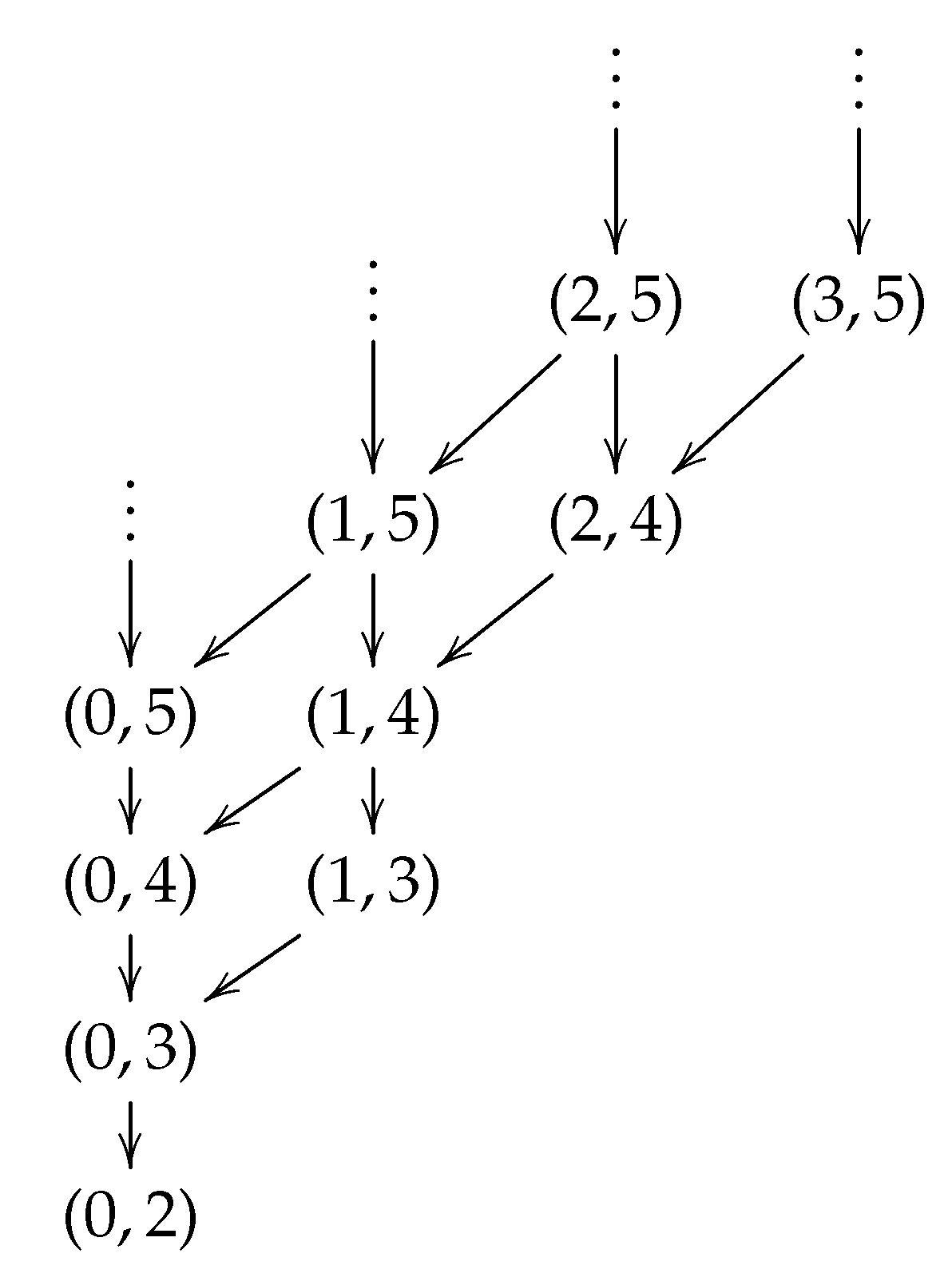
Figure 1, where each pair of numbers ( c , d ) represents the valuation x = c , y = d . The arrows show the < dl relations among them. In this case, there exists a unique clingo[dl]-answer set corresponding to the valuation x = 0 , y = 2 .

5.3. clingo[lp]

A third AMT system covered by our formalization is clingo[lp]. In this case, the abstract theory R is about linear equations over reals. It is identical to L but structured by ( X R , D R , vars L , · L ) where X R is an infinite set of real variables and the domain D R is the set of real numbers R . Previous versions of clingo[lp] treated either all theory atoms as external, E = T , or founded, E = . Since it imposes no restriction on the occurrence of linear equation atoms; the counter-intuitive behavior identified in [14] may emerge. The current version behaves like clingo[dl] and treats body atoms as external and head atoms as founded. Another commonality with clingo[dl] is a selection among the R , E -answer sets that are printed. In the case of clingo[lp], the selection is configurable by the user via a directive with a linear term:
& minimize { w 1 x 1 ; . . . ; w n x 1 }
where { w 1 , , w n } R and { x 1 , , x n } X R . Then, the partial order lp between two R , E -answer sets ( Y , v ) and ( Y , v ) is defined as:
( Y , v ) lp ( Y , v ) iff Y = Y and domain ( v ) = domain ( v ) and w 1 v ( x 1 ) + + w n v ( x n ) w 1 v ( x 1 ) + + w n v ( x n )
Similarly, we write ( Y , v ) < lp ( Y , v ) when ( Y , v ) lp ( Y , v ) and v v .
Definition 7 (clingo[lp]-answer set).
A R , E -answer set ( Y , v ) is called aclingo[lp]-answer set ofP if ( Y , v ) is < lp -minimal among the R , E -answer sets of P.
If no minimize directive is provided, the linear term x 1 + + x n with { x 1 , , x n } = X R is assumed by default. That is, the answer set with the smallest sum of variables is selected. For instance, given the program & sum { x } > = 0 , clingo[lp] only outputs the answer set where x = 0 .

6. Discussion and Related Work

There exist different hybrid approaches in the literature that combine logical inference with non-Boolean external theories that, in most cases, are related to some form of numerical constraints. When we combine logic programs and external theories, we may find two different philosophies that we can call black box versus white box orientations, respectively. In black box approaches, the intricacies of the external theory are mostly unknown from the logic program perspective: this is, in fact, the AMT approach followed in this paper. The white box style relies instead on extending the logic programming syntax to incorporate new structures and defining their corresponding semantics, treating constraints and their variables as first-class citizens inside the logic programming paradigm. Each orientation has its pros and cons. Black box approaches allow for a more flexible and homogeneous integration of new external theories, plus a simpler adaptation to new versions or features of the solvers. White box approaches are more convenient if we want to study formal properties of hybrid systems, such as equivalence among different representations or the soundness of syntactic transformations.
We proceed now to describe related work classified under these two orientations.

6.1. Black Box Orientation

Black box approaches follow somehow similar steps to what happened in SAT with the SAT modulo theories (SMT) [7] variant. SMT is defined as an extension to SAT where some atoms are replaced by formulas from some external theory expressible in first-order logic with equality, but usually without quantifiers (this includes numerical constraints but also covers data structures such as lists or strings). The key point in SMT is that the SAT solver does not really need to inspect the behavior of the external theory, so it can be treated as a black box. It is worth mentioning that, in fact, under the formalization proposed in the current paper, SMT can be seen as a particular case of AMT where all theory atoms are external (and we have no undefined variables) whereas, for each regular atom a , we include a choice rule such as (13), as we would do when emulating SAT inside ASP.
Following similar steps to SMT, the combination of constraint programming (CP) and ASP gave birth to Constraint Answer Set Programming (CASP). As explained in survey [18], CASP covers a family of approaches whose implementation may rely either on integration of CP inside a native ASP engine or on a translation of CASP programs into SMT or CP instead. From the semantic point of view, most of them treat theory atoms as external. Moreover, a choice for the constraint atom or its complement is usually included in the definitions. Moreover, many approaches only allow constraint atoms in bodies, e.g., in [5,19], or when they are used in rule heads [9], they just stand for syntactic sugar and can be shifted to bodies, as performed for clingcon-programs.
Next, we briefly list some of the existing CASP systems (see [18] for more examples) and their distinctive features with respect to the AMT framework proposed in this paper. Three examples of tools based on translation to non-ASP solvers are dingo [20], mingo [21], and ezsmt [22]. As happens with clingo[dl], system dingo [20] deals with ASP modulo difference logic but is actually based on a translation into SMT. In dingo, theory atoms are not external (they need to be derived), but they do not completely fit into our category of defined either, in the sense that SMT variables cannot be undefined. System ezsmt [22] is also based on a translation into SMT but accepts linear and non-linear constraints over mixed real and integer variables, whereas mingo [21] translates ASP modulo mixed-integer linear programming (MILP) to plain MILP. In these two systems, all theory atoms are external and may only appear in the body.
When solvers rely on the integration of constraints into native ASP instead, it is more common to find theory atoms that are defined rather than external. A prototypical example of this is ezcsp [19], where all theory atoms are defined and may only occur in the head, deviating from the standard CASP definition.
Another black box approach that extends ASP with external sources is HEX programs [23]. One of the main features of HEX programs is that, when consulting an external source, they allow higher-order parameters using the name of a logic program predicate as an argument for the external call. Another important feature is that HEX theory atoms allow for the invention of constants that are provided by the external source and were not originally present in the HEX program. This exceeds the ground-level definition used in the current paper. Yet, if we focus on ground HEX programs, we can observe that theory atoms only occur in rule bodies, and they do not require justification, so they would vaguely correspond to our external atom category. However, there are two important differences. First, it is unclear what the “complement” of a HEX theory atom would be or even if such a complement would make sense. Second, the truth of a HEX theory atom depends on the current interpretation handled by the logic program. Generally speaking, the information flow in most AMT systems is from the abstract theory T to the logic program but not in the other direction, that is, we usually have an abstract theory T whose behavior is known beforehand and is independent of the current stable model X. In principle, our definitions do not prevent dealing with a parameterized theory T X , but this option deserves to be explored in detail and will be part of future work.
One final and, perhaps, extreme example of a black box approach is the case of Multi-Context Systems (MCS) [24] where, rather than using ASP as basic formalism, we may actually deal with multiple contexts, each one with a potentially different logical formalism (classical logic, default logic, ASP, description logics, etc.). Like our description of abstract theories, the MCS logical formalisms are described at a very abstract level, only requiring the set of well-formed knowledge bases (the syntax), the set of belief sets, and the semantics in terms of a function that assigns the set of acceptable beliefs for each knowledge base. These contexts are connected altogether using so-called bridge rules, and the final semantics assigned to the system are defined in terms of equilibria reached among the belief sets from the contexts and the application of the bridge rules. The main difference with respect to MCS is that in AMT, we assume that our base formalism is ASP extended with other external theories and that, in principle, there is no particular interrelation among those theories or their shared beliefs.

6.2. White Box Orientation

In this second group of approaches, constraints are incorporated as first-class citizens inside the logic programming formalism, so their semantics are no longer external or abstract but are captured in an extended definition of answer sets. Examples of this orientation are a family of approaches [25,26,27] based on the incorporation of intensional or non-Herbrand functions in ASP. This line was initiated in [25] with the introduction of partial intensional functions in Quantified Equilibrium Logic, something that was later extended to sets and aggregates in [28]. This approach is very expressive as it provides full first-order semantics for arbitrary first-order formulas dealing with equality, functions, sets, and aggregates, but no implementation has followed from these definitions so far. Extending ASP with intensional functions was also considered in [29] and later on gave rise to the language ASP { f } [26]. These semantics were proven in [30] to be a particular case of [25] for a syntactic fragment where function nesting is restricted but had the advantage of allowing implementation with the system clingo { f } [31]. In these approaches, the treatment of functions is closer to the defined external atoms in the current paper: that is, functions can be undefined, and they can be used in rule heads to derive their value. However, in general, these semantics are more general in the sense that defined functions can also be used in rule bodies without the requirement of converting them into external. Another strongly related approach based on intensional functions is ASP(MT) [27], whose main difference with respect to [25] is that partial functions are not allowed (functions are always assigned a value). Again, Ref. [30] explains the relation between the two formalisms in detail and establishes a correspondence for a syntactic fragment where functions are not nested.
Another approach that can be classified as a white box system is s(CASP) [32], which is more aligned with the tradition of Constraint Logic Programming (CLP) inherited from Prolog. s(CASP) is a top-down query-based CASP system where constraint atoms may only occur unnegated in rule bodies. Here, constraints are defined in terms of predefined (usually arithmetic) operations performed on regular logic program variables, whose values are assumed to be just numeric elements in the Herbrand domain. This means that the definition of constraints only makes sense at a non-ground level. The semantics in CLP systems is normally defined in operational terms, and constraints are stored and solved on the fly during the goal-directed execution of rules. Comparison to AMT is difficult since constraints are represented in a substantially different manner: in AMT, they constitute external atoms that can be treated at the ground level (at least from the logic program perspective), whereas in s(CASP), constraints are always defined in terms of first-order variables. One difference that can be mentioned is that since logical variables cannot be undefined, s(CASP) does not produce results in which functions have no assigned value.
Finally, another approach that proposes a full, white-box treatment of constraints is ASP ( AC ) , recently introduced by [33]. ASP ( AC ) relies on an extension of the logic HT to deal with hybrid logic programs. Here, the orientation is the opposite of the previous approaches in this subsection. Rather than incorporating new operations in a first-order logical language, the logical connectives are generalized as particular cases of more general operations on weighted formulas over semi-rings. This means that, for instance, logical conjunction ∧ becomes just one more possible operation that can be combined with others, such as addition or multiplication (depending on the underlying semi-ring). This provides a very expressive and powerful formalism but at the price of a more complex semantic and the requirement of a semi-ring structure. Still, ASP ( AC ) covers a wide range of constructs, such as aggregates over non-Boolean variables, linear constraints, or provenance in positive Datalog programs.

7. Summary

We elaborated upon the formal foundations of hybrid ASP systems, focusing on extensions of clingo with different forms of linear equations. To this end, we extended logic programs with very general abstract theories without any predefined syntax. To characterize the interplay between theory atoms and their corresponding constraints, we extended the semantics of such programs and distinguished between defined and external theory atoms. Defined theory atoms have to be derived by the logic program for the represented constraint to take effect, while external theory atoms can be seen as oracles for which no justification inside the logic program is needed. A further refinement of abstract theories to structured ones allowed us to distinguish variables inside theory atoms and to assign values to them, leading to a denotation-based semantic. Moreover, this allows us to refine our extended concept of stable models with witnesses provided by assignments for theory variables. We then used the resulting concept of answer sets to characterize the semantic foundations of clingo’s hybrid extensions. Finally, we analyzed commonalities and differences to existing approaches of extending logic programs with external non-Boolean theories. These can be separated into black-box and white-box orientations, where in the former, the logic program is largely unaware of the intricacies of the external theory, while in the latter, the external theory is integrated into the logic programming syntax and semantics. The approach in this paper follows a black-box orientation, as the syntax of abstract and structured theories is completely left open and stable models are merely sanctioned by the external theory.

Author Contributions

P.C., J.F., T.S. and P.W. participated evenly in all stages of producing this work. All authors have read and agreed to the published version of the manuscript.

Funding

This work was supported by DFG grant SCHA 550/11, Germany, by grant PID2020-116201GB-I00 funded by MCIN/AEI/ 10.13039/501100011033, Spain, by Xunta de Galicia and the European Union, GPC ED431B 2022/33, by European COST action CA17124 DigForASP, EU, and by the National Science Foundation (NSF 95-3101-0060-402), USA.

Data Availability Statement

Not applicable.

Conflicts of Interest

The authors declare no conflict of interest.

Appendix A. Examples of Abstract Theories

Next, we define a family of abstract theories that encode some propositional logic, having a common set of theory atoms T p r of the form & prop { φ } for any propositional formula φ that can be formed for a set of variables X p r = { p , q , }, standing for propositional atoms, and with a fixed complement & prop { φ } = def & prop { ¬ φ } .
Example A1 (Equilibrium logic).
Take the abstract theory E = T p r , S , · with set S contains every set S of atoms whose set of formulas Γ = { φ & prop { φ } S } has some equilibrium model and negation as complement, as explained above. For a formal definition of Equilibrium Logic, we refer to [17]: for theories in the form of logic programs (as the ones we comment on below), it suffices to observe that equilibrium models coincide with stable models. As we can see, in this context, theory atoms talk about the inclusion of formulas φ (or their negation ¬ φ ) in an external logical theory Γ. For instance, we could write a program like:
& prop { ¬ q p } a & prop { ¬ p q }
Theory atom & prop { ¬ p q } is external: if we add it to the program, we obtain a stable model X 1 containing both theory atoms plus the propositional atom a . In fact, X 1 is also a E -stable model since the induced logical theory Γ 1 = { ( ¬ p q ) , ( ¬ q p ) } has (two) equilibrium models. If we do not include the external atom, stable model X 2 would just contain the defined atom & prop { ¬ q p } . This stable model does not pass the E -check since when we add the complement of the external atom, we get a logical theory Γ 2 = { ( ¬ p q ) , ¬ ( ¬ q p ) } that has no equilibrium model (The formula ¬ ( ¬ q p ) is HT -equivalent to ¬ q ¬ p ).
Note that the abstract entailment relation | T for this abstract theory does not satisfy monotonicity. For instance, & prop { ¬ p q } | T & prop { q } because adding the complement & prop { ¬ q } to & prop { ¬ p q } produces no equilibrium model. Yet, if we extend the theory with atom p, this is not true anymore, namely { & prop { ¬ p q } , & prop { p } } | T & prop { q } does not hold.
Example A2 (Kleene’s three-valued logic).
As an example of compositional theory without an absolute complement, consider K for capturing Kleene’s three-valued propositional logic. We define K with the same syntax (theory atoms and complement) as E , with the only difference that S now contains every set S of atoms such that Γ = { φ & prop { φ } S } has some three-valued model. For the denotations, we have D U = { 0 , 1 , 1 2 } and v φ iff f v ( φ ) = 1 for the evaluation function f v recursively defined as:
  • f v ( ) = def 0 , f v ( ) = def 1
  • f v ( x ) = def v ( x ) for atoms x X p r
  • f v ( φ ψ ) = def min ( f v ( φ ) , f v ( ψ ) )
  • f v ( φ ψ ) = def max ( f v ( φ ) , f v ( ψ ) )
  • f v ( ¬ φ ) = def 1 f v ( φ )
  • f v ( φ ψ ) = def f v ( ¬ φ ψ )
As an example, the denotation of atom p would correspond to:
& prop { p } K = { ( p = 1 , q = 0 ) , ( p = 1 , q = 1 / 2 ) , ( p = 1 , q = 1 ) }
and the denotation of its complement is:
& prop { ¬ p } K = { ( p = 0 , q = 0 ) , ( p = 0 , q = 1 / 2 ) , ( p = 0 , q = 1 ) }
but as we can see, there are valuations, such as ( p = 1 / 2 , q = 0 ) , that are not included in either of the two.
Example A3. 
Imagine that, in K , we added the operator M φ such that
f v ( M φ ) = def 0 if f v ( φ ) = 0 1 otherwise
that can then be read as “p is not false”. Then & prop { M p } | K & prop { p } since Γ = { M p , ¬ p } is unsatisfiable because no valuation v can assign f v ( M p ) = 1 and f v ( ¬ p ) = 1 simultaneously. However, regular entailment is not satisfied, & prop { M p } | K & prop { p } , because there are valuations in & prop { M p } K (anyone assigning 1 / 2 to p) that are not in & prop { p } K .
Example A4 (ukasiewicz Fuzzy logic).
Let us consider F for capturing ukasiewicz Fuzzy Logic. We define F with the same syntax (theory atoms and complement) as before, but S now contains every set S of atoms such that Γ = { φ & prop { φ } S } has some model in Fuzzy Logic. For the denotations, we have D F = [ 0 , 1 ] as an interval over real numbers, and v φ iff f v ( φ ) = 1 for the evaluation function f v recursively defined as:
  • f v ( ) = def 0 , f v ( ) = def 1
  • f v ( x ) = def v ( x ) for atoms x X p r
  • f v ( φ ψ ) = def min ( f v ( φ ) , f v ( ψ ) )
  • f v ( φ ψ ) = def max ( f v ( φ ) , f v ( ψ ) )
  • f v ( ¬ φ ) = def 1 f v ( φ )
  • f v ( φ ψ ) = def min ( 1 , 1 f v ( φ ) + f v ( ψ ) )
We conclude with an example of abstract theory that covers Description Logic ALC (other variants of Description Logics can be analogously defined). The most relevant feature, in this case, is that both variables and domain elements are partitioned into objects, concepts, and roles.
Example A5 (Description Logic ALC ).
Let us consider D for capturing Description Logics (DL). The set of variables X , in this case, is partitioned into object names X o , concept names X c , and role names X r . The set D is also partitioned into Δ 2 Δ 2 Δ × Δ , where Δ is a non-empty set representing all the objects in the Description Logic domain. Moreover, valuations v : X D are also partitioned so that v : X o Δ maps each object name to some element in Δ, v : X c 2 Δ maps each concept name to some subset of Δ, and v : X r 2 Δ × Δ maps each role name to some binary relation or set of pairs of elements from Δ. The theory atoms have the form & dl { φ } where φ is an assertion corresponding to one of the expressions:
φ : : = C C C C o : C ( o , o ) : R
being o , o X o and C some concept expression following the grammar:
C : : = A | C C | R . C | R | ¬ C
for any A X c and R X r . As we did before, to define the denotations, we use an evaluation function f v that, in this case, is used to map any concept expression C into some set of elements in Δ, that is, f v ( C ) Δ . This function is recursively defined as follows:
f v ( A ) = def v ( A ) for any concept name A X c f v ( C D ) = def f v ( C ) f v ( D ) f v ( R . C ) = def { x Δ for all y : ( x , y ) v ( R ) implies y f v ( C ) } f v ( R ) = def { x Δ there exists y such that ( x , y ) v ( R ) } f v ( ¬ C ) = def Δ f v ( C )
Finally, the denotation of a DL theory atom & dl { φ } is then defined as follows:
& dl { C D } = def { v f v ( C ) f v ( D ) } & dl { C D } = def { v f v ( C ) = f v ( D ) } & dl { o : C } = def { v v ( o ) f v ( C ) } & dl { ( o , o ) : R } = def { v ( v ( o ) , v ( o ) ) v ( R ) }

Appendix B. Proofs of Results

Proof of Proposition 1.
It is enough to show that
( S ( E S ) ) ( E ( S ( E S ) ) ) = ( S ( E S ) )
Note that A B = A B and A B = A B . Then,
( E ( S ( E S ) ) ) = ( E ( S ( E S ) )
Pick a ( E ( S ( E S ) ) ) . Then, a E and a ( S ( E S ) ) . The latter implies that a S . Hence, a E S = E S .
Then, we have that S is a T , E -solution that implies S ( E S ) is T -satisfiable by definition. Due to ( S ( E S ) ) ( E ( S ( E S ) ) ) = ( S ( E S ) ) , we know that S ( E S ) is E -complete and ( S ( E S ) ) ( E ( S ( E S ) ) ) is also T -satisfiable, then ( S ( E S ) ) is a E -complete T , E -solution.
Conversely, if S is a E -complete T , E -solution, then S ( E S ) = S is T -satisfiable by definition of E -complete and T , E -solution. □
Proof of Proposition 2.
Suppose, for the sake of contradiction, that there exists an incomplete T , E -solution S. Then, S S ( E S ) and, thus, there exists a theory atom s ( E S ) with s E , s S and s S . Furthermore, s E implies { s , s } E since E is closed. Then, s ( E S ) since s S and s E . This leads to a contradiction because { s , s } ( E S ) , and, therefore, S ( E S ) is not T -satisfiable. Since T is consistent, this implies that S is not a T , E -solution, which is a contradiction with the assumption that S is a T , E -solution. Consequently, all T , E -solutions S are E -complete for consistent abstract theory T and closed E . □
Lemma A1. 
Let P be a T -logic program and T = T , S , · be an abstract theory. Let E T be a set of external atoms, and let s E be one of those external atoms. Let S be a T , E -solution and let P be the program in (3). Then, X is a stable model of program
P { s B } { s s S } { s s S }
iff X is a stable model of program
P { ¬ s , B } { s s S }
Proof. 
We proceed by cases. Case 1. Assume that s S . Then, (A1) is
P { s B } { s }
which is strongly equivalent [34] to P { s } . Similarly, (A2) is
P { ¬ s , B } { s }
which is also strongly equivalent to P { s } . Case 2. Assume that s S . Then, (A1) is
P { s B } { s }
which is strongly equivalent to
P { B } { s }
In this case, (A2) is
P { ¬ s , B }
Case 2.1. Assume that s H ( P ) . Then, ( s ) P and, thus, (A4) can be rewritten as
P { ¬ s , B } { s }
Programs (A3) and (A5) are strongly equivalent. Case 2.2. Assume that s H ( P ) . Then, any stable model X of (A3) and (A4) must satisfy s X . Hence, X is a stable model of (A3) and a stable model of (A4). □
Proof of Proposition 3.
Let X A T be a set of atoms. We prove that X is a T , E -stable model of program P 1 = P { s B } iff X is a T , E -stable model of P 2 = P { ¬ s , B } . Let P be the program in (3). By definition, X is a T , E -stable model of P 1 = P { s B } iff there is a T , E -solution S such that X is a stable model of program
P 1 { s s ( S E ) } { s s ( T H ( P 1 ) ) S } = P { s B } { s s ( S E ) } { s s T S } = P { s B } { s s S } { s s S }
if and only if (Lemma A1) there is a T , E -solution S such that X is a stable model of program
P 2 { s s ( S E ) } { s s ( T H ( P 2 ) ) S } = P { ¬ s , B } { s s ( S E ) } = P { ¬ s , B } { s s S }
iff X is a T , E -stable model P 2 = P { ¬ s , B } . □
Proof of Proposition 4.
By construction, for every L -satisfiable set S S , we have s S s L . Then, there exists a valuation v s S s L and v s L for every s S . This implies that L is compositional.
Let us show that L is consistent. Suppose, for the sake of contradiction, that there exists a L -satisfiable set S S such that { s , s } S for a s T . Then, since L is compositional (as shown above), there has to exist a valuation, v, such that v s and v s . By definition of the denotation · T , this implies that v needs to satisfy both 1 i n c i v ( x i ) c 0 and 1 i n c i v ( x i ) c 0 , which is a contradiction. Therefore, every L -satisfiable set S S is consistent, and then L is consistent. □
Proof of Proposition 5.
We proceed by contraposition: suppose S T s T and S | / T s . Then S s is satisfiable, that is, there exists a valuation v S T s . However, then, on the one hand, v s S s T and the latter is included in s T , so we obtain v s T . On the other hand, v s T and so v s T s T , meaning that { s , s } is satisfiable and contradicts the consistency of T . □
Proof of Proposition 6.
Since T is compositional, proving ( S { s } ) S amounts to checking S { s } T = .
For the left to right direction, S | = T s is equivalent to S T s T . However, then S T s T s T s T = and so S T s T = S { s } T = .
For the right to left direction, we proceed by contraposition. Suppose there is some v S T such that v s T . If the complement is absolute, the latter means v s T and so v S T s T = S { s } T and so S { s } T . □
Proof of Proposition 7.
Let X be some T , E -stable model. By definition, there is some T , E -solution S such that X is a stable model of the program in (3). By construction of this program, it follows S E = X E and S F X F . In addition, since S is a T , E -solution, it follows that S is T -satisfiable (S is complete by Proposition 2 and the fact that E is closed). Let S = X T . Then, S S and, since T is compositional and S is T -satisfiable, it follows that S is also T -satisfiable. That is, there is some valuation, v, such that v s for all s S = X T . Let v be the partial valuation that is only defined in vars ( S ) , and that satisfies v ( x ) = v ( x ) for all x vars ( S ) . Then, v | vars ( X T ) s T | vars ( X T ) for all s S = X T and, thus, pair ( X A , v ) belongs to ans ( X ) . □
Proof of Proposition 8.
We start by showing that, if ( Y , v ) is a T , E -answer set, then stb P ( Y , v ) is a T , E -stable model X of P such that ( Y , v ) belongs to ans ( X ) .
Since ( Y , v ) is a T , E -answer set, there is a stable model X such that ( Y , v ) belongs to ans ( X ) . We will show that stb P ( Y , v ) = X . By definition,
stb P ( Y , v ) A = Y = X A stb P ( Y , v ) E = s E v s T | domain ( v ) X E stb P ( Y , v ) F = s F ( B s ) P and ( Y , v ) | = T B
Let us now show that
stb P ( Y , v ) E = s E v s T | domain ( v ) X E
Pick any theory atom s E such that s X . Since X is a stable model, there is some T , E -solution S such that X is a stable model of the program in (3). By construction of program (3), this implies s S . Furthermore, since E is closed, S is complete (Proposition 2) and thus, both s S and s X follow. Then, v s T | domain ( v ) and since the complement is absolute, it follows that v s T | domain ( v ) . Hence, s stb P ( Y , v ) E and
stb P ( Y , v ) E = X E
Let us now show that
stb P ( Y , v ) F = s F ( B s ) P and ( Y , v ) | = T B = X F
Pick s X F . Then, there is a rule ( B s ) P such that b X for b B A and b X for ¬ b B and b A . This implies that b Y for b B A and b Y for ¬ b B and b A and, thus, ( Y , v ) | = T b and ( Y , v ) | = T ¬ b . Furthermore, for every b B T , we have b X and, by construction, v s T | domain ( v ) and thus ( Y , v ) | = b . Similarly, for every ¬ b B and b T it holds that v s T | domain ( v ) and, therefore, ( Y , v ) | = ¬ b . This implies that ( Y , v ) | = T B and, thus, that s stb P ( Y , v ) F . Now, the other way around. Pick s F such that ( B s ) P and ( Y , v ) | = T B . Then, B A Y X , b Y for ¬ b B and b A implying b X , v b T | domain ( v ) for b B T implying b X T , and, v b T | domain ( v ) for ¬ b B and b T implying b X T . Therefore, X satisfies rule body B and must include s since X is a stable model of P. Hence, s X F and stb P ( Y , v ) F = X F follows. Consequently, stb P ( Y , v ) = X is a T , E -stable model of P.
Therefore, we get the following correspondences
( Y , v ) ans ( stb P ( Y , v ) ) for any T , E - answer set ( Y , v ) { stb P ( Y , v ) ( Y , v ) ans ( X ) } = { X } for any T , E - stable model X
It is easy to see that stb P ( · ) and ans ( · ) establish one-to-one correspondence between the T , E -stable models of P and the equivalence classes with respect to P of its T , E -answer sets. □

References

  1. Lifschitz, V. Thirteen Definitions of a Stable Model. In Fields of Logic and Computation, Essays Dedicated to Yuri Gurevich on the Occasion of His 70th Birthday; Lecture Notes in Computer Science; Blass, A., Dershowitz, N., Reisig, W., Eds.; Springer: Berlin, Germany, 2010; Volume 6300, pp. 488–503. [Google Scholar] [CrossRef] [Green Version]
  2. Gelfond, M.; Lifschitz, V. The Stable Model Semantics for Logic Programming. In Proceedings of the Fifth International Conference and Symposium of Logic Programming (ICLP’88), Seattle, WA, USA, 15–19 August 1988; Kowalski, R., Bowen, K., Eds.; MIT Press: Cambridge, MA, USA, 1988; pp. 1070–1080. [Google Scholar] [CrossRef]
  3. Gebser, M.; Harrison, A.; Kaminski, R.; Lifschitz, V.; Schaub, T. Abstract Gringo. Theory Pract. Log. Program. 2015, 15, 449–463. [Google Scholar] [CrossRef] [Green Version]
  4. Falkner, A.; Friedrich, G.; Schekotihin, K.; Taupe, R.; Teppan, E. Industrial Applications of Answer Set Programming. Künstliche Intell. 2018, 32, 165–176. [Google Scholar] [CrossRef] [Green Version]
  5. Lierler, Y. Relating constraint answer set programming languages and algorithms. Artif. Intell. 2014, 207, 1–22. [Google Scholar] [CrossRef]
  6. Kaminski, R.; Schaub, T.; Wanko, P. A Tutorial on Hybrid Answer Set Solving with clingo. In Proceedings of the Thirteenth International Summer School of the Reasoning Web, London, UK, 7–11 July 2017; Lecture Notes in Computer Science. Ianni, G., Lembo, D., Bertossi, L., Faber, W., Glimm, B., Gottlob, G., Staab, S., Eds.; Springer: Berlin, Germany, 2017; Volume 10370, pp. 167–203. [Google Scholar] [CrossRef]
  7. Barrett, C.; Sebastiani, R.; Seshia, S.; Tinelli, C. Satisfiability Modulo Theories. In Handbook of Satisfiability; Frontiers in Artificial Intelligence and Applications; Chapter 26; Biere, A., Heule, M., van Maaren, H., Walsh, T., Eds.; IOS Press: Amsterdam, The Netherlands, 2009; Volume 185, pp. 825–885. [Google Scholar] [CrossRef]
  8. Elkabani, I.; Pontelli, E.; Son, T. Smodels with CLP and Its Applications: A Simple and Effective Approach to Aggregates in ASP. In Proceedings of the Twentieth International Conference on Logic Programming (ICLP’04), Saint-Malo, France, 6–10 September 2004; Lecture Notes in Computer Science. Demoen, B., Lifschitz, V., Eds.; Springer: Berlin, Germany, 2004; Volume 3132, pp. 73–89. [Google Scholar] [CrossRef]
  9. Gebser, M.; Ostrowski, M.; Schaub, T. Constraint Answer Set Solving. In Proceedings of the Twenty-Fifth International Conference on Logic Programming (ICLP’09), Pasadena, CA, USA, 14–17 July 2009; Lecture Notes in Computer Science. Hill, P., Warren, D., Eds.; Springer: Berlin, Germany, 2009; Volume 5649, pp. 235–249. [Google Scholar] [CrossRef]
  10. Drescher, C.; Walsh, T. A Translational Approach to Constraint Answer Set Solving. Theory Pract. Log. Program. 2010, 10, 465–480. [Google Scholar] [CrossRef] [Green Version]
  11. Ostrowski, M.; Schaub, T. ASP modulo CSP: The clingcon system. Theory Pract. Log. Program. 2012, 12, 485–503. [Google Scholar] [CrossRef] [Green Version]
  12. De Rosis, A.; Eiter, T.; Redl, C.; Ricca, F. Constraint Answer Set Programming Based on HEX-Programs. In Proceedings of the Eighth Workshop on Answer Set Programming and Other Computing Paradigms (ASPOCP’15), Cork, Ireland, 13 August 2015; Inclezan, D., Maratea, M., Eds.; 2015. [Google Scholar]
  13. Banbara, M.; Kaufmann, B.; Ostrowski, M.; Schaub, T. Clingcon: The Next Generation. Theory Pract. Log. Program. 2017, 17, 408–461. [Google Scholar] [CrossRef] [Green Version]
  14. Janhunen, T.; Kaminski, R.; Ostrowski, M.; Schaub, T.; Schellhorn, S.; Wanko, P. Clingo goes Linear Constraints over Reals and Integers. Theory Pract. Log. Program. 2017, 17, 872–888. [Google Scholar] [CrossRef] [Green Version]
  15. Eiter, T.; Germano, S.; Ianni, G.; Kaminski, T.; Redl, C.; Schüller, P.; Weinzierl, A. The DLVHEX System. Künstliche Intell. 2018, 32, 187–189. [Google Scholar] [CrossRef]
  16. Gebser, M.; Kaminski, R.; Kaufmann, B.; Ostrowski, M.; Schaub, T.; Wanko, P. Theory Solving Made Easy with Clingo 5. In Proceedings of the Technical Communications of the Thirty-Second International Conference on Logic Programming (ICLP’16), New York, NY, USA, 16–21 October 2016; pp. 2:1–2:15. [Google Scholar]
  17. Pearce, D. Equilibrium logic. Ann. Math. Artif. Intell. 2006, 47, 3–41. [Google Scholar] [CrossRef]
  18. Lierler, Y. Constraint Answer Set Programming: Integrational and Translational (or SMT-based) Approaches. Theory Pract. Log. Program. 2023, 23, 195–225. [Google Scholar] [CrossRef]
  19. Balduccini, M.; Lierler, Y. Constraint answer set solver EZCSP and why integration schemas matter. Theory Pract. Log. Program. 2017, 17, 462–515. [Google Scholar] [CrossRef] [Green Version]
  20. Janhunen, T.; Niemelä, I.; Sevalnev, M. Computing Stable Models via Reductions to Difference Logic. In Proceedings of the Tenth International Conference on Logic Programming and Nonmonotonic Reasoning (LPNMR’09), Potsdam, Germany, 14–18 September 2009; Lecture Notes in Artificial Intelligence. Erdem, E., Lin, F., Schaub, T., Eds.; Springer: Berlin, Germany, 2009; Volume 5753, pp. 142–154. [Google Scholar]
  21. Liu, G.; Janhunen, T.; Niemelä, I. Answer Set Programming via Mixed Integer Programming. In Proceedings of the Thirteenth International Conference on Principles of Knowledge Representation and Reasoning (KR’12), Rome, Italy, 10–14 June 2012; Brewka, G., Eiter, T., McIlraith, S., Eds.; AAAI Press: Palo Alto, CA, USA, 2012; pp. 32–42. [Google Scholar]
  22. Lierler, Y.; Susman, B. SMT-Based Constraint Answer Set Solver EZSMT (System Description). Comput. Sci. Fac. Proc. Present. 2016, 46, 1:1–1:15. [Google Scholar]
  23. Eiter, T.; Ianni, G.; Schindlauer, R.; Tompits, H. A Uniform Integration of Higher-Order Reasoning and External Evaluations in Answer-Set Programming. In Proceedings of the Nineteenth International Joint Conference on Artificial Intelligence (IJCAI’05), Scotland, UK, 30 July–5 August 2005; Kaelbling, L., Saffiotti, A., Eds.; Morgan Kaufmann Publishers Inc.: Burlington, VT, USA, 2005; pp. 90–96. [Google Scholar]
  24. Brewka, G.; Eiter, T. Equilibria in Heterogeneous Nonmonotonic Multi-Context Systems. In Proceedings of the Twenty-Second National Conference on Artificial Intelligence (AAAI’07), Vancouver, BC, Canada, 22–26 July 2007; AAAI Press: Palo Alto, CA, USA, 2007; pp. 385–390. [Google Scholar]
  25. Cabalar, P. Functional answer set programming. Theory Pract. Log. Program. 2011, 11, 203–233. [Google Scholar] [CrossRef] [Green Version]
  26. Balduccini, M.; Gelfond, M. Language ASP{f} with Arithmetic Expressions and Consistency-Restoring Rules. arXiv 2013, arXiv:1301.1387. [Google Scholar]
  27. Bartholomew, M.; Lee, J. First-order stable model semantics with intensional functions. Artif. Intell. 2019, 273, 56–93. [Google Scholar] [CrossRef]
  28. Cabalar, P.; Fandinno, J.; Fariñas del Cerro, L.; Pearce, D. Functional ASP with Intensional Sets: Application to Gelfond-Zhang Aggregates. Theory Pract. Log. Program. 2018, 18, 390–405. [Google Scholar] [CrossRef] [Green Version]
  29. Balduccini, M. A “conservative” approach to extending answer set programming with nonherbrand functions. In Correct Reasoning: Essays on Logic-Based AI in Honour of Vladimir Lifschitz; Lecture Notes in Computer Science; Erdem, E., Lee, J., Lierler, Y., Pearce, D., Eds.; Springer: Berlin, Germany, 2012; Volume 7265, pp. 24–39. [Google Scholar]
  30. Bartholomew, M.; Lee, J. On the stable model semantics for intensional functions. Theory Pract. Log. Program. 2013, 13, 863–876. [Google Scholar] [CrossRef] [Green Version]
  31. Balduccini, M. ASP with non-herbrand partial functions: A language and system for practical use. Theory Pract. Log. Program. 2013, 13, 547–561. [Google Scholar] [CrossRef] [Green Version]
  32. Arias, J.; Carro, M.; Salatar, E.; Marple, K.; Gupta, G. Constraint Answer Set Programming without Grounding. Theory Pract. Log. Program. 2018, 18, 337–354. [Google Scholar] [CrossRef] [Green Version]
  33. Eiter, T.; Kiesel, R. ASP(AC): Answer Set Programming with Algebraic Constraints. Theory Pract. Log. Program. 2020, 20, 895–910. [Google Scholar] [CrossRef]
  34. Lifschitz, V.; Pearce, D.; Valverde, A. Strongly equivalent logic programs. ACM Trans. Comput. Log. 2001, 2, 526–541. [Google Scholar] [CrossRef]
Figure 1. Answer sets for (18) without negative values.
Algorithms 16 00185 g001
Disclaimer/Publisher’s Note: The statements, opinions and data contained in all publications are solely those of the individual author(s) and contributor(s) and not of MDPI and/or the editor(s). MDPI and/or the editor(s) disclaim responsibility for any injury to people or property resulting from any ideas, methods, instructions or products referred to in the content.

