All articles published by MDPI are made immediately available worldwide under an open access license. No special
permission is required to reuse all or part of the article published by MDPI, including figures and tables. For
articles published under an open access Creative Common CC BY license, any part of the article may be reused without
permission provided that the original article is clearly cited. For more information, please refer to
https://www.mdpi.com/openaccess.
Feature papers represent the most advanced research with significant potential for high impact in the field. A Feature
Paper should be a substantial original Article that involves several techniques or approaches, provides an outlook for
future research directions and describes possible research applications.
Feature papers are submitted upon individual invitation or recommendation by the scientific editors and must receive
positive feedback from the reviewers.
Editor’s Choice articles are based on recommendations by the scientific editors of MDPI journals from around the world.
Editors select a small number of articles recently published in the journal that they believe will be particularly
interesting to readers, or important in the respective research area. The aim is to provide a snapshot of some of the
most exciting work published in the various research areas of the journal.
In many tasks related to an object’s observation or real-time monitoring, the gathering of temporal multimodal data is required. Such data sets are semantically connected as they reflect different aspects of the same object. However, data sets of different modalities are usually stored and processed independently. This paper presents an approach based on the application of the Algebraic System of Aggregates (ASA) operations that enable the creation of an object’s complex representation, referred to as multi-image (MI). The representation of temporal multimodal data sets as the object’s MI yields simple data-processing procedures as it provides a solid semantic connection between data describing different features of the same object, process, or phenomenon. In terms of software development, the MI is a complex data structure used for data processing with ASA operations. This paper provides a detailed presentation of this concept.
Humans perceive real-world objects through the multiple senses. Semantic fusion of multi-type (multimodal) information about the object of observation received using multi-channel sensing is a natural process for the human brain. Following this natural principle, many scientific and engineering tasks also require complex semantic descriptions of an object of study based on the fusion of multimodal data received from multiple devices.
In many cases, the object is supervised over the course of time. Such timewise observation can help in understanding the dynamics of the object’s behavior and is necessary in many applications. Then, such a timewise complex description requires a collection of multimodal data that are obtained from several sensors measuring certain parameters of the object’s behavior, cameras recording the appearance of the object, etc., over time, not necessarily received simultaneously. This brings the problem of correct multimodal data representation based on data synchronization and aggregation.
Another aspect of using multimodality is its employment for object recognition. The latest advancement in this area concerns multimodal machine learning, which involves integrating and modeling information from multiple heterogeneous sources of data [1]. However, this approach reveals several challenges related to heterogeneity of the data.
According to [2], the first fundamental challenge is comprehensive data representation that takes into consideration the complementarity and redundancy of multiple modalities. The second challenge is multimodal data mapping that enables matching data of different modalities. The third challenge is data alignment that consists of the necessity to identify direct relations between elements from different modalities. The fourth challenge is data fusion, which yields united information of different modalities. The fifth challenge is co-learning, which consists of transferring knowledge based on different modalities. As stated in [1], there are even more challenges that include reasoning, generation, and quantification, along with data representation, alignment, and transference. All these and related issues require correct and comprehensive multimodal data representation, which is key to overcoming challenges related to different aspects of multimodal data analysis and processing.
The rest of the paper is organized as follows. Section 2 presents a related work review. Section 3 formulates the requirements of temporal multimodal data processing and explains the need to employ the Algebraic System of Aggregates (ASA) for the formal specification of an object. Section 4 explains the basic concepts of the ASA. Section 5 provides a detailed presentation of the algorithms of operations on aggregates. Section 6 presents the notion of a multi-image of an object and proposes an algorithm for multi-image formation. Section 7 offers a use case and provides the discussion of ASA operations application for multi-image formation. Finally, Section 8 concludes the paper.
2. Related Work
There are a number of papers presenting different approaches and views on the task of data fusion/data aggregation in various contexts.
Jesus et al. [3] formally defined the concept of aggregation, reviewed distributed data aggregation algorithms, and provided taxonomy of the main aggregation techniques. Comparing different techniques in their survey, the authors showed that among main data aggregation classes, the hierarchical-based approach is the cheapest option; the sketch-based approach could be considered fast but not very precise; the averaging technique gives a higher level of precision but with a much slower execution, which might not be very efficient to operate on dynamic networks, although very few approaches would actually be practical when there are dynamic settings, which presents a challenge for further research on improvements in the efficiency of dynamic networks.
Ribeiro et al. [4] proposed an algorithm for intelligent information fusion in uncertain environments, named fuzzy information fusion (FIF), which is based on multi-criteria decision making and computational intelligence. In this study, data fusion was considered a process of aggregating data from multiple sources into a single composite with higher information quality. The authors analyzed various methods of data fusion. While they considered fuzzy Set theory to be of high applicability, it needs application domain knowledge for data representation, which makes this method not fully universal and creates room for further research in this direction.
Oliveira et al. [5] presented an application of the fuzzy information fusion algorithm for the aggregation of various sources of heterogeneous information to generate value-added maps. In their work, they used operators from different classes of operators, such as algebraic, average, and reinforcement, to fuse, e.g., aggregate data. Validation with specific scenarios allowed authors to compare aggregation operators. The multiplicative FIMICA operator was identified as the most consistent operator that gave the best classification outputs for the scenarios used. It shows, however, that for certain use cases, there is a need for specialized operators that yield efficiently aggregated data depending on a specific scenario.
Lahat et al. [6] considered data fusion to be “the analysis of several data sets such that different data sets can interact and inform each other” and studied multimodality as a form of diversity. In the paper, the authors focused their attention on different aspects of multimodality, considering it in the context of various applications. They also outlined the importance of the development of single-set analysis methods for advanced data fusion.
Marinoni et al. [7] considered data fusion in the context of image pre-processing with relation to transfer learning in remote sensing. In their paper, the authors proposed metrics that quantify the maximum information extraction performance to be achieved by multimodal remote-sensing analysis. Empirical outcomes presented in the paper demonstrated how the accuracy performance of a standard classifier applied to a multimodal data set can be improved using the reliability metric. The approach proposed by the authors can be used to improve multimodal remote-sensing information extraction.
Gaonkar et al. [8] provided a study on advancements in multimodal signal processing. In the paper, focus was given to multimodal data representation and information fusion. The authors considered information fusion based on model-agnostic and model-based approaches.
Oliveira et al. [9] focused on the application of data fusion in a decision support system (DSS). The effectiveness of such a system depends on reliable fusion of data coming from multiple sources. The paper proposed high-level architecture of the DSS.
As was stated in the Introduction, one of the promising applications of multimodality is multimodal machine learning (MML). This topic stimulated a number of resent research works.
Liang et al. [10] discussed the foundational principles in multimodal research and, in particular, the principle of heterogeneity and the principle of interconnection. The authors also provided taxonomy of six core challenges in multimodal machine learning (representation, alignment, reasoning, generation, transference, and quantification) and gave their comprehensive analysis. They outlined different aspects of these challenges, and some of them are of particular interest in the context of the research purposes of this paper. Specifically, modality connections and interconnections, as an essential part of multimodal models, can show how modalities are related and how their elements interact. There is, however, a need, which the authors pointed out as one of the future directions, to formally define the core principles of heterogeneity, connections, and interactions. It requires a mathematical framework to be able to capture causal, logical, and temporal connections and interactions, which formulates a mathematical and algorithmic problem to consider.
Guo et al. [11] studied deep multimodal representation learning frameworks, including modality-specific representations, joint representation and coordinated representation, and encoder–decoder framework. They outlined one of the challenges that still exists in the context of machinery comprehension of information from multiple sensory organs, which is the heterogeneity gap in multimodal data. Aiming to narrow this gap, the authors summarized some typical models in deep multimodal representation learning, including probabilistic graphical models, multimodal autoencoders, deep canonical correlation analysis, generative adversarial networks, and attention mechanisms. Their analysis of different learning frameworks showed that one of the main disadvantages of existing frameworks and models is the difficulty of coordinating more than two modalities. It formulates a practical challenge for further research to overcome the issue of multiple modalities.
Baltrusaitis et al. [2] provided an overview of the recent advances in multimodal machine learning and presented a summary of applications enabled by multimodal machine learning. In their work, they introduced taxonomy of multimodal machine learning, which includes five core challenges: representation, translation, fusion, alignment, and co-learning. Some of these challenges have already been studied quite well. In contrast, there are a few more recent ones (e.g., representation and translation), which are now leading the creation of new multimodal algorithms and are still of interest for further research.
Kline et al. [12] provide a summary of multimodal data fusion applications for solving medical diagnostics problems. The paper shows how medical data of different modalities (e.g., text/image, EHR/genomic/time series) recorded and extracted can be used in a specific use case, giving a firm understanding of the practical importance of multimodal data processing.
3. Approach and Requirements for Temporal Multimodal Data Processing
In our research, we consider an approach to temporal multimodal data processing based on the formal specification of the objects under study. For this purpose, we need a theoretical apparatus to provide the logic of presentation and processing of temporal multimodal data at the level of mathematics, algorithms, and software, taking into account such features of this data:
Multimodality means that the object is determined by a collection of data of a different nature; the logic of presenting and processing data about the object depends on the qualitative and quantitative composition of the data set.
Temporality means that the elements of data collection are ordered by the time of their receiving; the order of following individual elements of the data sequence affects the result of processing the entire set of data of the object.
The description of the object and the effective processing of temporal multimodal data require specific mathematical abstractions and mechanisms to operate them. The basic requirements for a mathematical apparatus to describe and process data include the possibility of the following:
Presenting a data set as a structure of semantically interconnected elements.
Considering the sequence of data set elements when performing logical operations on them.
Reordering elements of the data set.
Let us consider several candidates for a mathematical concept to meet these requirements. As the data are temporal, the first possible candidate is the theory of time series (TTS) [13,14]. The TTS is one of the branches of mathematical statistics that deals with the analysis of stochastic processes. The TTS enables the analysis of data sequences, as well as the study of trends, predictions, and other similar data processing. However, time series do not allow any logical operations of the data elements. Therefore, the TTS cannot be employed for logical processing of temporal multimodal data.
Two other candidates are the theory of sets (TS) [15] and the theory of multisets (TMS) [16,17]. Both of them provide flexible mechanisms for the logical processing of data sets; however, they do not consider the sequence of elements and, accordingly, do not provide the possibility of ordering the elements in a set of temporal multimodal data.
Thus, neither of the considered theories fully correspond to the needs of temporal multimodal data processing based on the formal specification of the objects under study. However, the abovementioned requirements are satisfied by the Algebraic System of Aggregates (ASA) [18,19]. This mathematical concept enables data processing with consideration of both required data features, namely multimodality and temporality (Table 1).
Let us consider the main provisions and possibilities of the ASA for the presentation and processing of temporal multimodal data describing an object.
4. Basics Notions of ASA
The ASA [18,19] is an algebraic system whose carrier is a non-empty set of objects, which we call aggregates.
Definition1.
An aggregate A is an ordered finite collection of elements defined by a tuple of setsand a tuple of tuples of elements, and the elementsof each tuple of elementsbelong to the corresponding set,, which specifies a one-to-one relationship between the sequence of sets and the sequence of tuples of elements:
whereis a tuple of sets;is a tuple of tuples of elements; andis a separate element (value) or a composite element (a tuple of homogeneous values or a tuple of heterogeneous values), .
The defining features of the aggregate, which distinguish this mathematical abstraction from others, are the following:
An aggregate is a complex mathematical object, all of whose components are ordered;
Elements of the tuples can be individual values or tuples of values, and the tuples of values can consist of both values of the same type and values of different types, while each tuple contains elements belonging to one set.
According to (1), the elements of the first tuple belong to the first set, the elements of the second tuple belong to the second set, etc. The sequence of sets in an aggregate determines how operations on the aggregate are performed. Sets in a tuple of sets can be repeated; this means that the aggregate includes several tuples consisting of elements of the same type. In software code, an aggregate can be defined as a data structure presented in Listing 1.
Listing 1. Interface of a data structure for representing an aggregate.
Aggregate structure: collection ← ordered collection of tuples length ← number of tuples in the aggregate Initialize Aggregate define length of the aggregate create collection of size length initialize tuples in collection Insertion (entity) ← add an entity, i.e., a set of values from different tuples Extraction (entity) ← delete the specific entity TupleInsertion (position) ← add a new tuple to the specific position in the aggregate TupleExtraction (position) ← delete the specific tuple AscendingSorting (primaryTuple) ← sort tuples in the aggregate by the defined primary tuple in asceding order DecendingSorting (primaryTuple) ← sort tuples in the aggregate by the defined primary tuple in descending order Singling (primatyTuple) ← remove all non-unique entities by the defined primary tuple SetsOrdering (orderOfTuples) ← reorder tuples by the defined order
As the order of elements in the aggregate is a crucial point in the ASA, the result of carrying out operations on aggregates depends on the aggregates’ compatibility.
Definition2.
Aggregatesandare called compatible () if they have the same length, and the type and sequence of sets in them match, that is, the conditions are met:
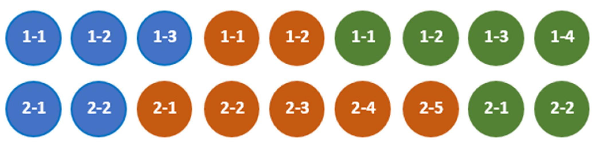
For example, the aggregates defined by (3) and illustrated by Figure 1 are compatible.
In Figure 1, the color of an element represents data modality (elements of set are blue, elements of set are brown and elements of set are green), the first value in the element’s number designates the aggregate ( or ), and the second value in the element’s number is an ordering number of the element in the tuple belonging to a certain set. For example, the blue circle, which contains the numbers 1-1, represents the element that belongs to the set from the definition of and the green circle, which contains the numbers 2-1, represents the element that belongs to the set from the definition of .
Definition3.
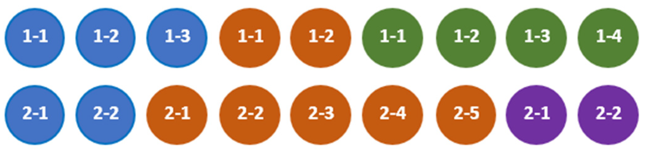
Aggregatesandare called quasi-compatible () if the type and sequence order of the sets in them partially coincide, while there is no requirement for the equality of the lengths of these aggregates, i.e., the conditions are fulfilled:
For example, the aggregates defined by (5) and illustrated by Figure 2 are quasi-compatible.
Definition4.
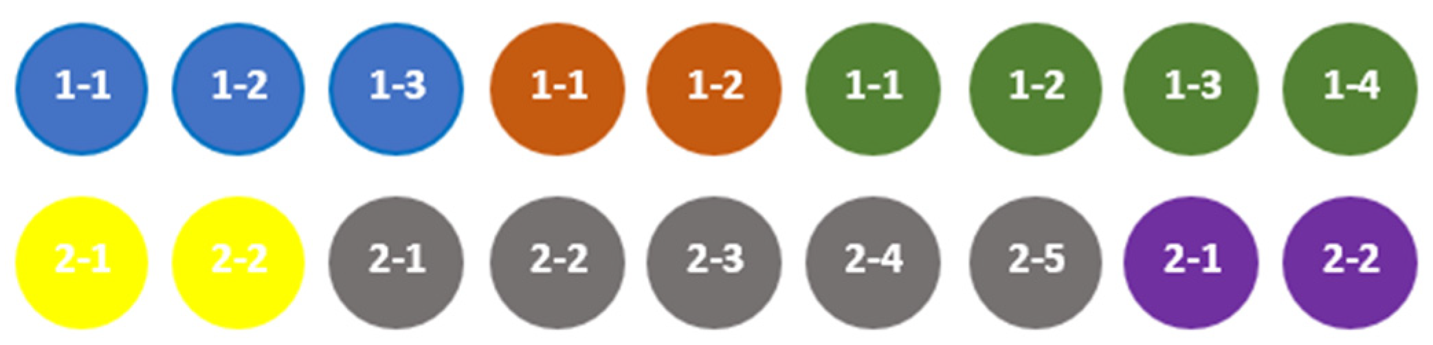
Aggregatesandare called incompatible (), if the type and sequence of the sets in them do not match, that is, the condition is fulfilled:
For example, the aggregates defined by (7) and illustrated by Figure 3 are incompatible.
A special case of incompatibility is hidden compatibility.
Definition5.
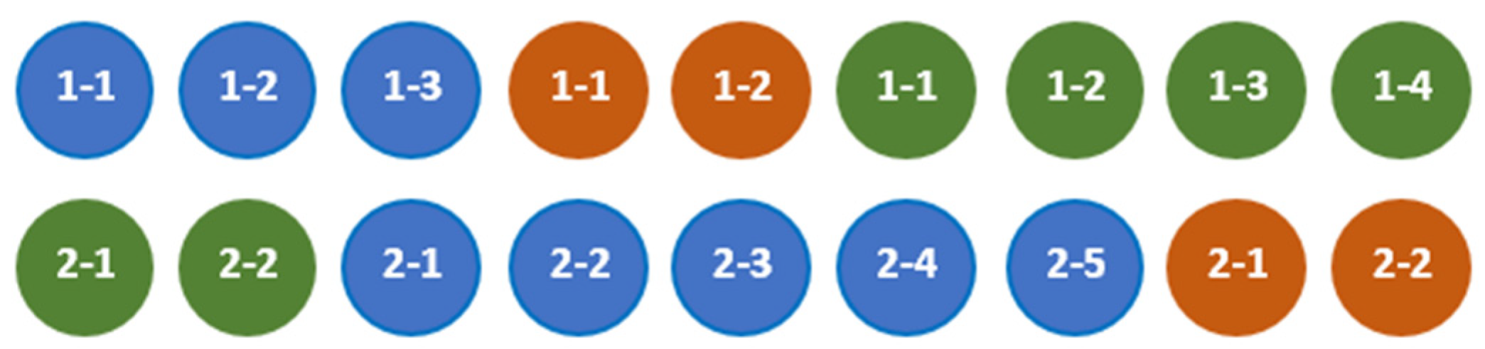
Aggregatesandare called hiddenly compatible,, if both aggregates have the same set of sets, but their ordering is different, i.e., the conditions are fulfilled:
where , .
For example, the aggregates defined by formulas (9) and illustrated by Figure 4 are hiddenly compatible.
Hiddenly compatible aggregates can be made compatible by applying certain operations to them.
5. Algorithms of Operations on Aggregates
The operations on aggregates in the ASA include logical operations, ordering operations, and arithmetic operations.
5.1. Logical Operations
The logical operations [18] on aggregates are union, intersection, exclusive intersection, difference, and symmetric difference. The result of any logical operation depends on the aggregates’ compatibility. For example, the rule for the union operation can be mathematically defined as follows.
The union of the aggregates and is the aggregate , which contains elements of the tuples that belong to both aggregates and are ordered in the following way:
1.
If , then aggregates and are defined as
and elements of i-tuple of the aggregate are added to the end of i-tuple of the aggregate :
2.
If , then aggregates and are defined as
(a) elements of the i-tuple of the aggregate are added to the end of the i-tuple of the aggregate , if the elements of these tuples belong to the same i-set;
(b) for all i-tuples whose elements belong to different sets, the tuple of tuples of aggregate is added to the end of the tuple of tuples of aggregate , and the tuple of sets of aggregate is added to the end of the tuple of sets of aggregate , with the exception of tuples subject to rule (a), which are excluded from the tuple of tuples:
3.
If , then aggregates and are defined as
the tuple of tuples of aggregate is added at to end of the tuple of tuples of the aggregate , and the tuple of sets of aggregate is added to the end of the tuple of sets of the aggregate :
The results of applying the union operation to two aggregates with different compatibility (Figure 1, Figure 2 and Figure 3) are shown in Figure 5.
This mathematical definition can be presented as the algorithm for finding a result of the union of two aggregates as shown in Listing 2.
Listing 2: Algorithm of the union operation for two aggregates.
Input: aggregates and Output: aggregate ifthen fordo fordo fordo end else ifthen fordo fordo else fordo if and then fordo fordo else
end end for end end
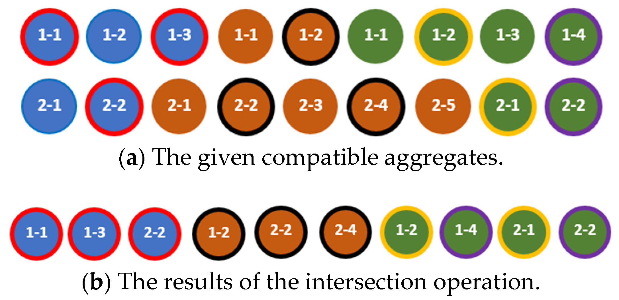
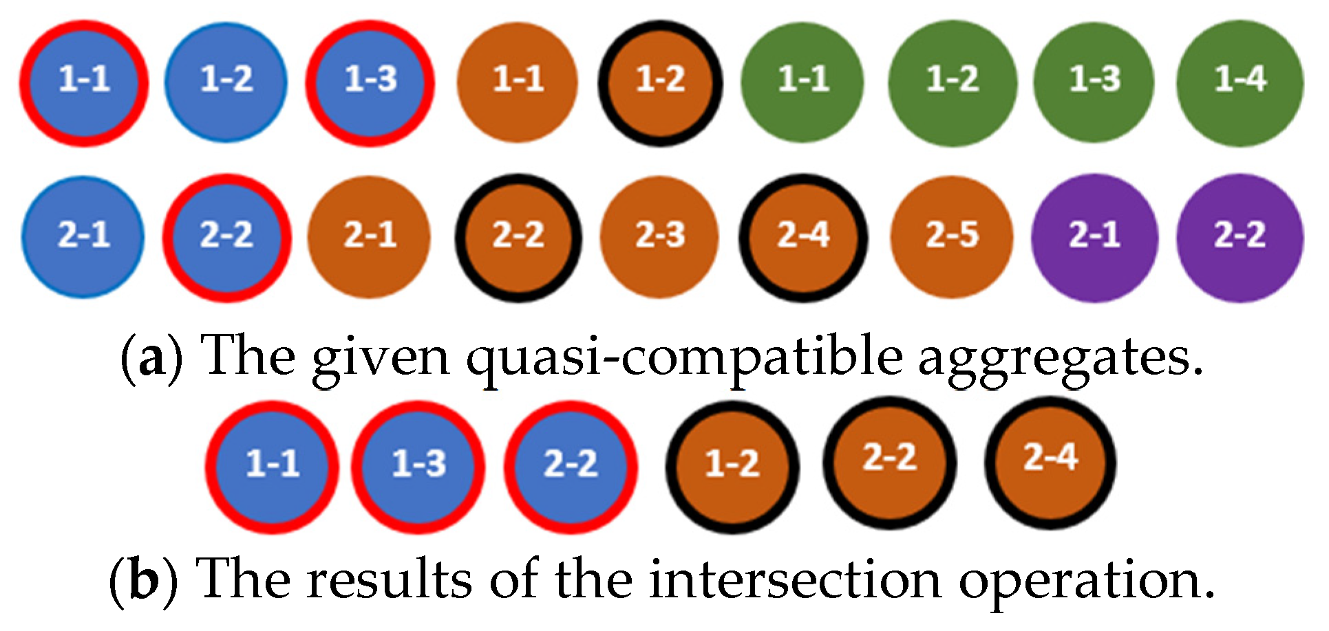
The intersection of the aggregates and is the aggregate , which contains components that are common to these aggregates and are ordered according to the rule defined in [18]. This rule can be presented as the algorithm for finding a result of the intersection of two aggregates as shown in Listing 3.
Listing 3: Algorithm of the intersection operation for two aggregates.
Input: aggregates and Output: aggregate ifthen fordo fordo if end end fordo if end end end else ifthen
else fordo if and then fordo if end end fordo if end end end end
The results of the intersection operation applied to the compatible and quasi-compatible aggregates are shown in Figure 6 and Figure 7, respectively. The elements of the same color marked with the same border color are equal, for example, (blue elements with the red border) in Figure 6.
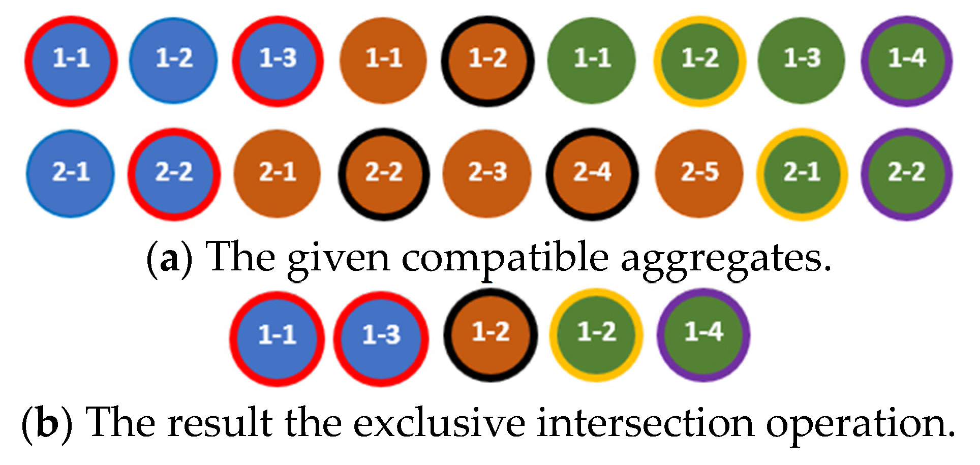
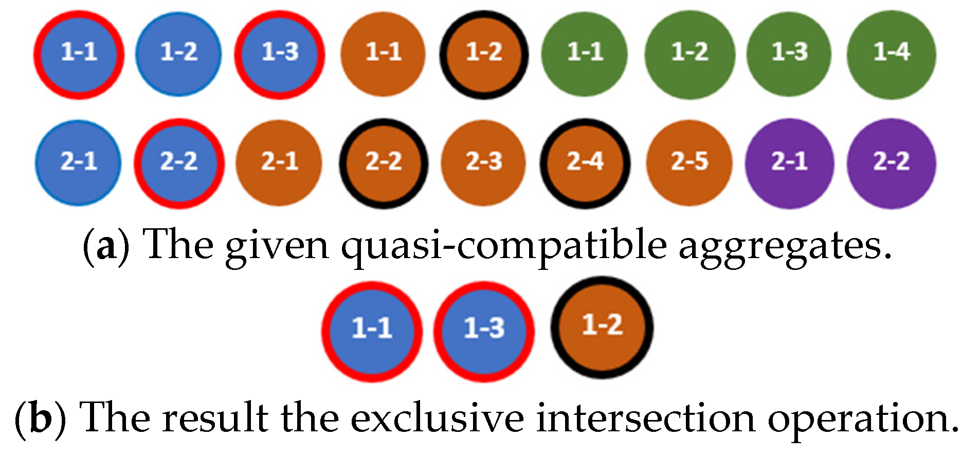
The exclusive intersection of the aggregates and is the aggregate , which contains only components of the aggregate that are common in these aggregates and are ordered according to the rule defined in [18]. This rule can be presented as the algorithm for finding a result of the exclusive intersection of two aggregates as shown in Listing 4.
Listing 4: Algorithm of the exclusive intersection operation for two aggregates.
Input: aggregates and Output: aggregate ifthen fordo fordo if end end end else ifthen
else fordo if and then fordo if end end end end
The results of the exclusive intersection operation applied to the compatible and quasi-compatible aggregates are shown in Figure 8 and Figure 9, respectively.
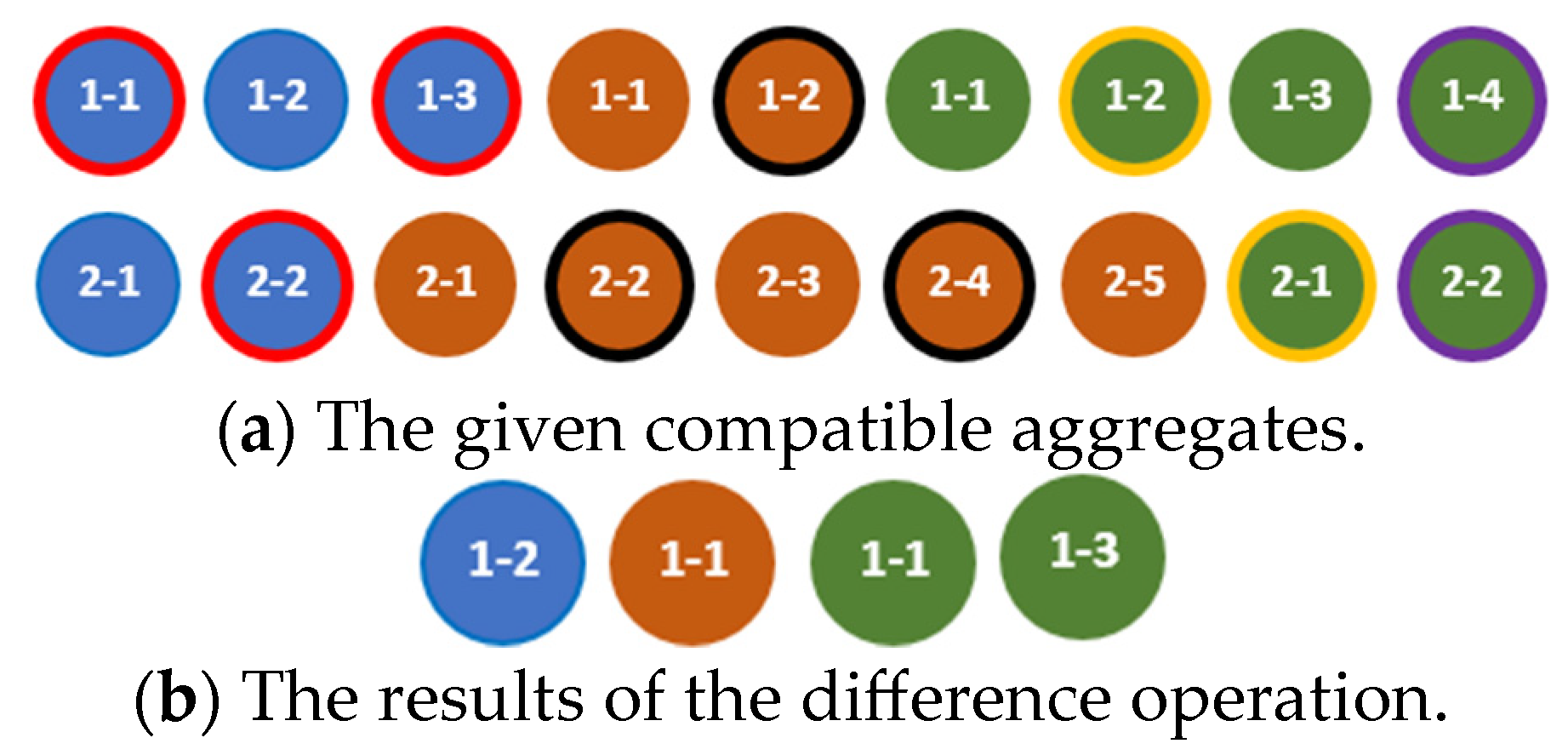
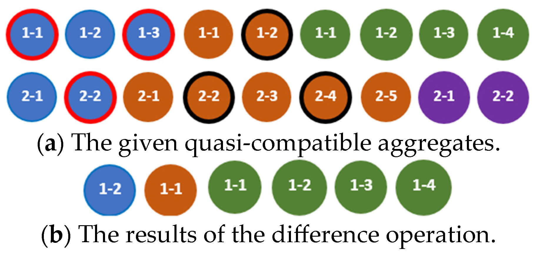
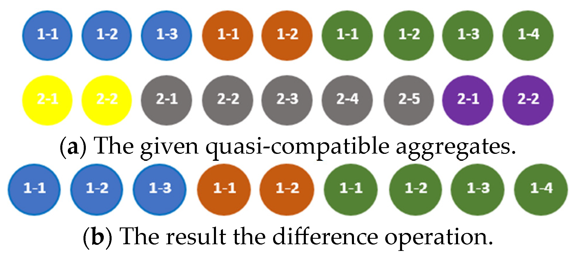
The difference of the aggregates and is the aggregate , which contains components of the aggregate that are not present in the aggregate and are ordered according to the rule defined in [18]. This rule can be presented as the algorithm for finding a result of the difference of two aggregates as shown in Listing 5.
Listing 5: Algorithm of the difference operation for two aggregates.
Input: aggregates and Output: aggregate ifthen fordo fordo if end end end else ifthen fordo
end else fordo if and then fordo if end end else
end end
The result of the difference operation applied to the compatible, quasi-compatible, and incompatible aggregates is shown in Figure 10, Figure 11 and Figure 12, respectively.
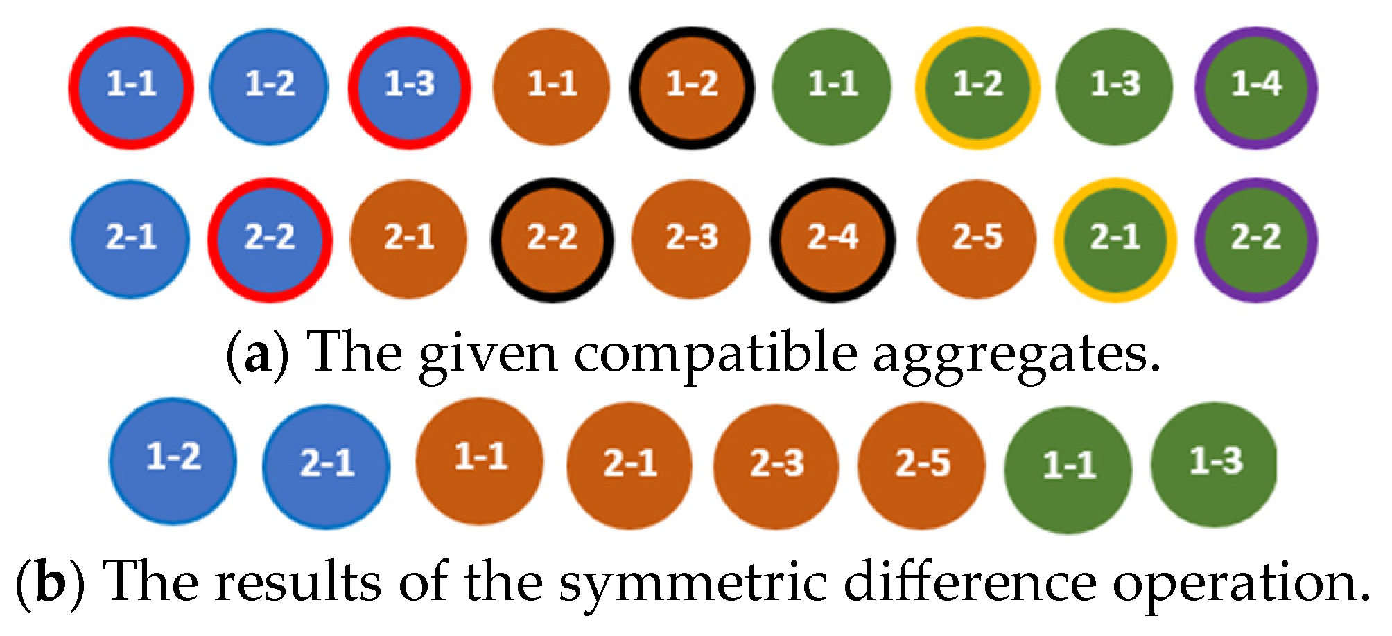
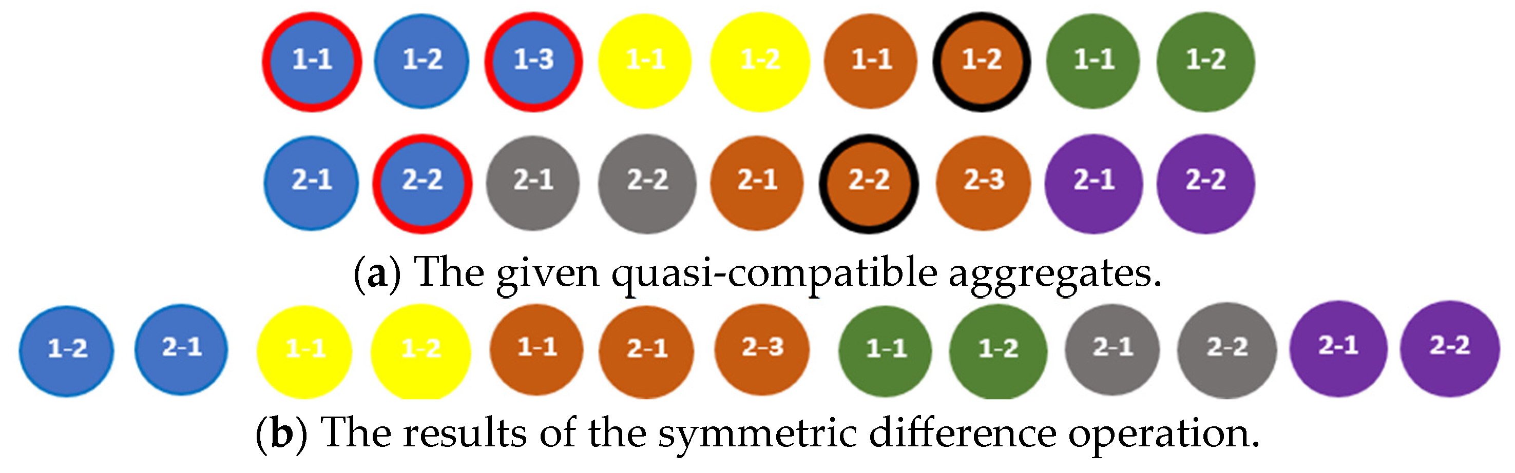
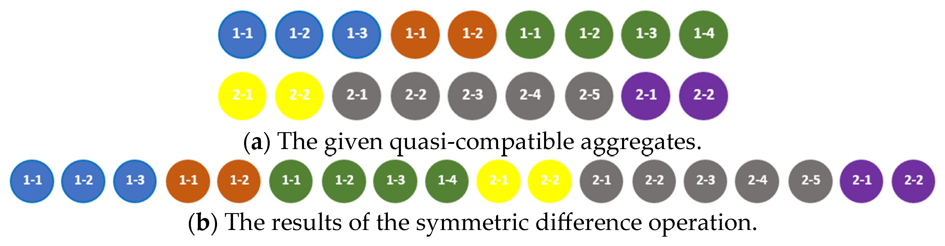
The symmetric difference of the aggregates and is the aggregate , which contains components of the aggregate that are not in the aggregate and components of the aggregate that are not in the aggregate , and are ordered according to the rule defined in [18]. This rule can be presented as the algorithm for finding a result of the symmetric difference of two aggregates as shown in Listing 6.
Listing 6: Algorithm of the symmetric difference operation for two aggregates.
Input: aggregates and Output: aggregate ifthen fordo fordo if end end fordo if end end end else ifthen fordo
end fordo
end else fordo if and then fordo if end end fordo if end end else
end end fordo
end end
The results of the symmetric difference operation applied to the compatible, quasi-compatible, and incompatible aggregates are shown in Figure 13, Figure 14 and Figure 15, respectively.
5.2. Ordering Operations
The ordering operations [19] on aggregates are sets ordering, sorting, singling, extraction, and insertion.
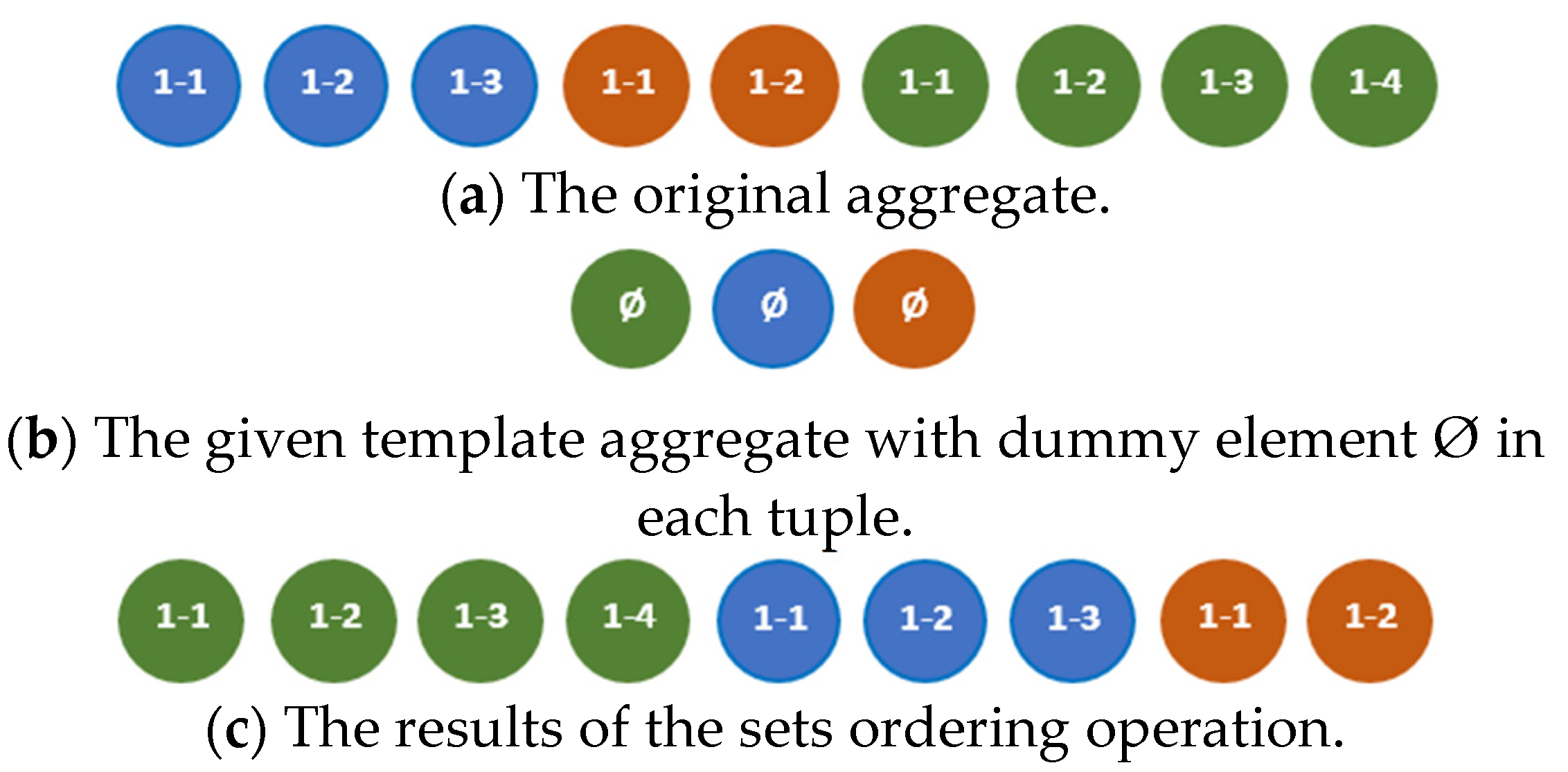
Sets ordering is an ordering operation that reorders the tuple of sets and the corresponding tuple of tuples of the aggregate , according to the given hiddenly compatible aggregate , which consists of any arbitrary elements, including dummy ones, as shown in Figure 16. The result of sets ordering is the aggregate
The sets ordering operation can be fulfilled according to the algorithm in Listing 7.
Listing 7. Algorithm of the sets ordering operation.
Input: aggregates and Output: aggregate while not ordered do
fordo ifthen
ifthen sets are ordered end end end end
The sets ordering operation has an important practical value that can be discovered through the following theorem and its corollary.
Theorem1.
The theorem on compatibility.
Ifand, thenandfor, such as .
Proof of Theorem1.
Let us consider two arbitrary hiddenly compatible aggregates and , i. e., , and apply the sets ordering operation to these aggregates in two ways as follows:
;
.
Let us consider the aggregates and . As is the result of applying the sets ordering operation, then by Definition 11, the result of its application to the given hiddenly compatible aggregates and is the aggregate , where , , which means .
According to Definition 1, the aggregate can be presented as .
According to Definition 5, two aggregates are hiddenly compatible if and , , .
Then, , , .
According to Definition 2, the aggregates and are compatible because and , which we would have to prove.
The compatibility of the aggregates of and can be proved analogously. □
Remark1.
The corollary of Theorem 1.
The practical significance of applying the sets ordering operation to hiddenly compatible aggregatesandis that the components of one aggregate () can be rearranged according to the sequence of the components of the second aggregate (); therefore, as a result of applying the sets ordering operation, the hiddenly compatible aggregates become compatible.
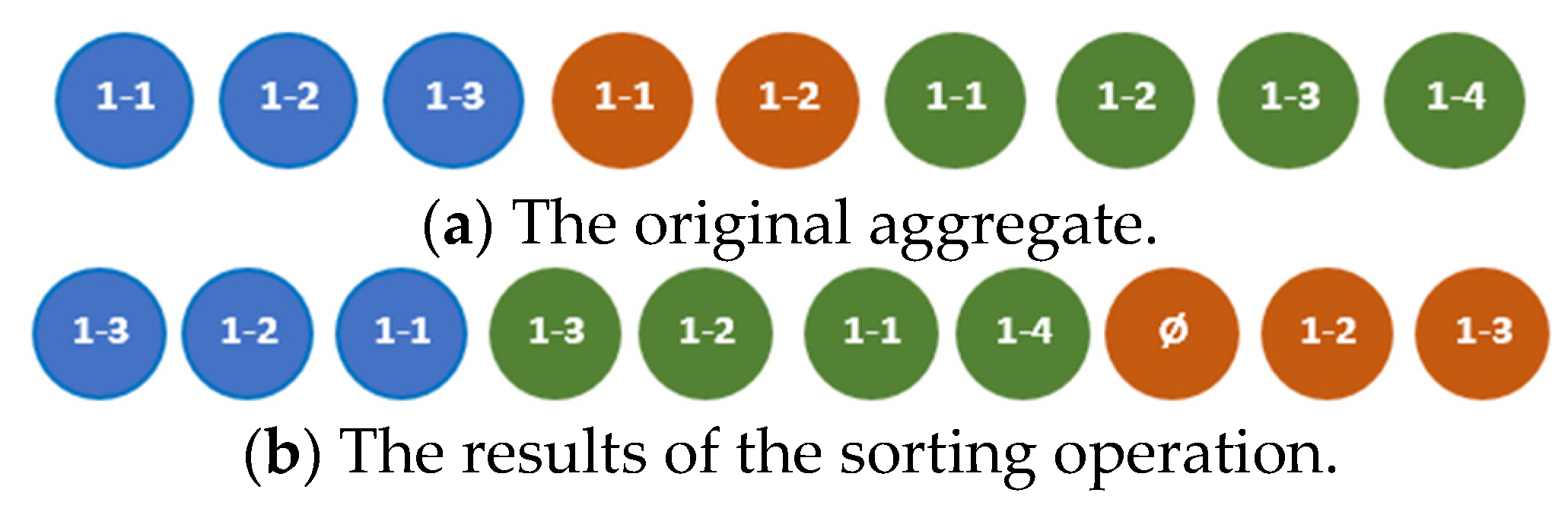
The sorting operation [19] yields a new (sorted) sequence of elements of a certain tuple named the primary tuple. The result of applying the sorting operation to an aggregate is an aggregate (for ascending sorting) or (for descending sorting) in all tuples, in which the elements are reordered according to the new ordering of the indices of the elements of the sorted primary tuple . If some tuple is shorter than the primary tuple, it is appended by a dummy element and is then sorted. If some tuple is longer than the primary one, the elements with indices that exceed the largest index in the primary tuple, are not sorted (remain on their positions). An example of the result of sorting operation is given in Figure 17.
The sorting operation can be realized using any appropriate sorting algorithm [20], including the one shown in Listing 8.
Listing 8: Algorithm of the ascending sorting operation.
Input: aggregate and primary tuple Output: aggregate fordo fordo swapped is false ifdo fordo
end swapped is true end end ifswapped is false break loop end end
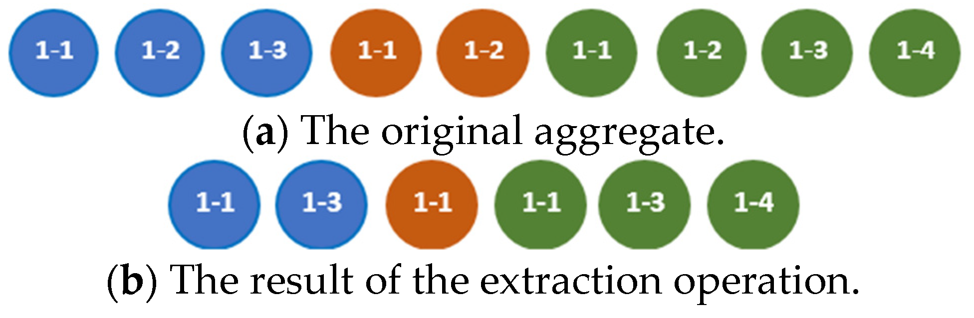
The extraction operation removes a certain element from the primary tuple of an aggregate. The result of extraction of the element from the aggregate is the aggregate in all tuples, from which the elements with index are removed.
An example of the result of the extraction operation for is given in Figure 18.
The extraction operation can be fulfilled according to the algorithm in Listing 9.
Listing 9: Algorithm of the extraction operation.
Input: aggregate , number of set and position of element Output: aggregate fordo fordo fordo end
The insertion operation adds a given element to the known position in the primary tuple of an aggregate. The result of insertion of the element to the aggregate is the aggregate in all tuples (except the primary one), to which dummy elements with index are added.
An example of the result of insertion of a new element to the second position of the primary tuple is shown in Figure 19, where the indices of the shifted elements remain as they numerated in the original tuple for explanatory purposes.
The insertion operation can be fulfilled according to the algorithm in Listing 10.
Listing 10: Algorithm of the insert operation.
Input: aggregate , number of set and position of element Output: aggregate fordo fordo
end ifthen
else
end fordo
end end
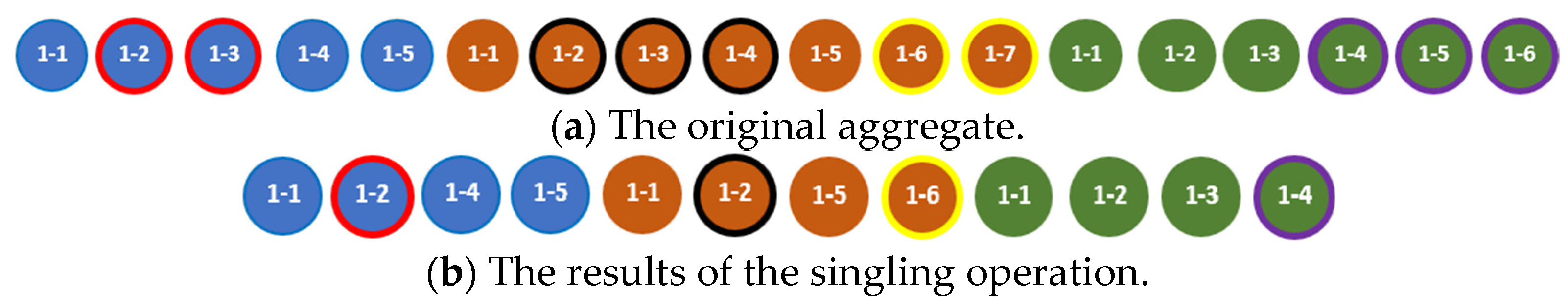
The singling operation removes the duplicate values that are located next to each other from the primary tuple of the aggregate; elements with the same indices as those of the removed duplicates in the primary tuple are simultaneously removed in all other tuples.
An example of the result of the singling operation is given in Figure 20. Elements of the same color marked with the same border color are equal.
The singling operation can be fulfilled according to the algorithm in Listing 11.
Listing 11: Algorithm of the singling operation.
Input: aggregate Output: aggregate m = 2 whilenot all founddo fordo ifthen
break loop end all found end fordo extract end end
6. Multi-Image Notion and Formation Algorithm
The multi-image concept [21] is an essential part of the approach presented in this paper as it enables the required formal description of the sequences of multimodal data about the object under study.
Definition6.
A multi-image is a non-empty aggregate specified as:
whereis a set of time values; .
From a practical point of view, multi-image refers to a structure of consolidated temporal multimodal data sets that describe different aspects of the same object. Let us formulate an algorithm that enables the formation of multi-image for an arbitrary object described through several temporal multimodal data sets.
The inputs to the algorithm of the object’s multi-image formation are temporal data sets and the data type (modality) of each set. The algorithm consists of seven steps. The result of the algorithm is multi-image, presented in the form of an ordered collection of temporal multimodal data.
The first step of the algorithm is the formalization of the object’s multi-image data structure. This step is performed according to the requirements for the object’s description. Multi-image can be defined mathematically, according to (13), or in any other way that allows a researcher to unambiguously specify the sequence of data sets and their modality.
At the second step of the algorithm, multi-image specification is decomposed into a set of specifications of partial multi-images as seen in (14).
where T is the set of time values; is the set of data values of -modality; ; ; and is the number of data sets.
At the third step, data are obtained. The procedure for receiving data involves determining the method (protocol, format) of data transmission, determining the time period for data transmission, establishing a connection with the data source and receiving data in a specified way and in a specified format.
At the fourth step, the data of each modality are prepared to form the corresponding partial multi-image. A partial multi-image is an aggregate that includes two tuples of elements, namely a tuple of time values and a tuple of elements of a certain modality. Elements are individual values or ordered sets of values (homogeneous or heterogeneous). Data preparation, which is performed at this step, consists of determining (detecting) time values in the set of data obtained at the previous stage. This procedure can be either trivial when the data format requires explicit presentation of time values for the temporal data component, or complex when the time values are presented in an implicit form or are ambiguous. A method for detecting hidden or ill-defined time values must be developed for each specific data format.
At the fifth step, partial multi-images are combined into a single multi-image. The multi-image merging procedure includes two actions: normalization and uniting.
1.
Normalization of partial multi-images (a normalized multi-image (normalized tuple) is a multi-image (tuple) to the elements of which dummy elements are added; a dummy element is a value that is absent in the tuple before its normalization; an empty element ∅ can be used as a dummy element; at other steps of the multi-image processing, dummy elements are ignored):
where is the insertion operation; is the number of dummy elements; ; is an element of a normalized tuple; and .
2.
Uniting the normalized partial multi-images:
At the sixth step, the multi-image obtained at the previous stage is sorted by the tuple of time values:
where and are indices specifying the order of the elements in the sorted tuple and .
At the seventh step, the sorted multi-image obtained at the previous step is singled by a tuple of time values:
where is the number of discarded time value duplicates.
The obtained I is the final multi-image that represents the consolidated data describing different aspects of the object under study.
7. Discussion
Let us consider a use case in the area of healthcare that demonstrates the practical use of the proposed approach of multimodal data processing (Figure 21).
The healthcare use case assumes that the data describing the patient’s health status can be obtained from multiple sources, including medical investigation devices (MRI scanners, CT scanners, ECG machines, etc.), manual medical measurement tools and devices (pulse oximeters, thermometers, sphygmomanometers, etc.), test systems (e.g., blood testing), and medical documentation records (treatment events). Data sets collected from these sources are temporal multimodal and semantically interconnected as they describe different features of the same object that is a patient’s organism. The multi-image concept and ASA operations can be employed to consolidate such a compound data collection and implement the logic of its processing.
Let us consider an example which demonstrates the formation of multi-image from several timewise data sequences according to the algorithm proposed in Section 6 and the algorithms of the ASA operations presented in Section 5.
Suppose that the patient’s blood pressure readings (systolic and diastolic), pulse rate, and oxygen saturation level are being measured several times a day. A pair of blood pressure values are to be received from the sphygmomanometer, and the values of pulse rate and oxygen saturation level are to be received from a pulse oximeter. The number of measurements conducted by the sphygmomanometer is ; the number of measurements conducted by the pulse oximeter is .
As a result of patient health parameters monitoring, the following multi-image must be obtained:
According to the algorithm of multi-image formation, the received data are represented as two partial multi-images—a partial multi-image containing values received from the first device (sphygmomanometer) and a partial multi-image containing values received from the second device (pulse oximeter):
To obtain the multi-image, these partial multi-images must be properly merged. For this purpose, at first, we need to normalize these partial multi-images, i.e., apply the insertion operation and add dummy elements to the end of the tuple of blood pressure values and to the beginning of both the tuple of heart rate values and the tuple of oxygen saturation level values:
After normalization, we apply the union operation to the normalized aggregates:
Next, we need to sort the obtained multi-image by the time tuple using the corresponding ASA operation:
The tuples are now ordered, but they include duplicate time values. To remove them, we apply the singling operation:
As a result, we obtain a multi-image that contains data from two independent but semantically interconnected examinations of the patient. This consolidated data structure can be used for further data processing.
This simple example demonstrates that the ASA offers operations which consider both data features defined in Section 3: multimodality (logical operations allow us to implement any logic for modality-wise data processing) and temporality (ordering operations enable timewise data processing). This principle of the proposed approach is valid for any data type because according to Definition 1, an aggregate can include both separate elements and composite elements (homogeneous or heterogeneous values).
The mathematical approach introduced in the ASA is implemented in the domain-specific programming language ASAMPL [22,23,24].
8. Conclusions
Algorithms for performing operations of the Algebraic System of Aggregates (ASA) are proposed in the paper. A feature of this algebraic system is the consideration of the sequence of elements (tuples, aggregates) when performing operations, including brand-new ordering operations. The properties of the ASA make it possible to use it for the formal description of objects under observation and for the development of methods for processing temporal multimodal data.
An algorithm for creating an object’s multi-image is also proposed in the paper. The input data for this algorithm are separate sets of temporal data. The algorithm consists of seven steps, which include the formation of the multi-image data structure of the object under study, decomposition of the multi-image specification into a set of partial multi-image specifications, obtaining and preparing separate data sets, combining partial multi-images into a single multi-image, sorting the multi-image, and thinning the sorted multi-image by tuple time values. The result of algorithm execution is a multi-image of an object containing synchronized and aggregated sequences of temporal multimodal data characterizing this object.
The proposed mathematical approach can be used for a formal description of digital models in various tasks, including a digital twin design, semantic model construction, and temporal multimodal data aggregation and processing. The mathematical concepts offered by the ASA can also be employed for the consolidation of data for multimodal data processing in multimodal machine learning tasks. Further work should aim to increasing the efficiency of the proposed algorithms.
Author Contributions
Conceptualization, A.P. and Y.S.; methodology, Y.S. and I.D.; software, O.S.; validation, A.P., Y.S. and I.D.; writing—original draft preparation, Y.S. and O.S.; writing—review and editing, A.P. All authors have read and agreed to the published version of the manuscript.
Funding
This research received no external funding.
Data Availability Statement
Not applicable.
Conflicts of Interest
The authors declare no conflict of interest.
References
Morency, L.-P.; Liang, P.P.; Zadeh, A. Tutorial on Multimodal Machine Learning. In Proceedings of the 2022 Conference of the North American Chapter of the Association for Computational Linguistics: Human Language Technologies: Tutorial Abstracts, Seattle, WA, USA, 10–15 July 2022; Association for Computational Linguistics: Stroudsburg, PA, USA, 2022; pp. 33–38. [Google Scholar]
Jesus, P.; Baquero, C.; Almeida, P.S. A Survey of Distributed Data Aggregation Algorithms. IEEE Commun. Surv. Tutor.2015, 17, 381–404. [Google Scholar] [CrossRef] [Green Version]
Ribeiro, R.A.; Falcão, A.; Mora, A.; Fonseca, J.M. FIF: A fuzzy information fusion algorithm based on multi-criteria decision making. Knowl.-Based Syst.2014, 58, 23–32. [Google Scholar] [CrossRef]
Oliveira, D.; Martins, L.; Mora, A.; Damásio, C.; Caetano, M.; Fonseca, J.; Ribeiro, R.A. Data fusion approach for eucalyptus trees identification. Int. J. Remote Sens.2021, 42, 4087–4109. [Google Scholar] [CrossRef]
Lahat, D.; Adali, T.; Jutten, C. Multimodal Data Fusion: An Overview of Methods, Challenges, and Prospects. Proc. IEEE2015, 103, 1449–1477. [Google Scholar] [CrossRef] [Green Version]
Marinoni, A.; Chlaily, S.; Jutten, C. Addressing Reliability of Multimodal Remote Sensing to Enhance Multisensor Data Fusion and Transfer Learning. In Proceedings of the International Geoscience and Remote Sensing Symposium (IGARSS 2020), Waikoloa, HI, USA, 26 September 2020; pp. 3896–3899. [Google Scholar] [CrossRef]
Gaonkar, A.; Chukkapalli, Y.; Raman, P.J.; Srikanth, S.; Gurugopinath, S. A Comprehensive Survey on Multimodal Data Representation and Information Fusion Algorithms. In Proceedings of the 2021 International Conference on Intelligent Technologies (CONIT), Hubli, India, 25–27 June 2021; pp. 1–8. [Google Scholar] [CrossRef]
Oliveira, J.P.; Lourenço, M.; Oliveira, L.; Mora, A.; Oliveira, H. A Data Fusion of IoT Sensor Networks for Decision Support in Forest Fire Suppression. In Internet of Things. Technology and Applications. IFIPIoT 2021; Camarinha-Matos, L.M., Heijenk, G., Katkoori, S., Strous, L., Eds.; IFIP Advances in Information and Communication Technology; Springer: Cham, Switzerland, 2022; Volume 641. [Google Scholar] [CrossRef]
Liang, P.P.; Zadeh, A.; Morency, L.-P. Foundations and Recent Trends in Multimodal Machine Learning: Principles, Challenges, and Open Questions. arXiv2023, arXiv:2209.03430. [Google Scholar] [CrossRef]
Guo, W.; Wang, J.; Wang, S. Deep Multimodal Representation Learning: A Survey. IEEE Access2019, 7, 63373–63394. [Google Scholar] [CrossRef]
Kline, A.; Wang, H.; Li, Y.; Dannis, S.; Hutch, M.; Xu, Z.; Wang, F.; Cheng, F.; Luo, Y. Multimodal machine learning in precision health: A scoping review. Npj Digit. Med.2022, 5, 171. [Google Scholar] [CrossRef] [PubMed]
Wei, W. Time Series Analysis; Pearson Addison Wesley: San Francisco, NY, USA, 2006; 614p. [Google Scholar]
Hannan, E.J. Multiple Time Series; John Wiley and Sons: Hoboken, NJ, USA, 2009; 535p. [Google Scholar]
Fraenkel, A.A.; Bar-Hillel, Y.; Levy, A. Foundations of Set Theory; Elsevier: Hoboken, NJ, USA, 1973; 415p. [Google Scholar]
Petrovsky, A.B. Structuring techniques in multiset spaces. In Multiple Criteria Decision Making; Springer: Berlin/Heidelberg, Germany, 1997; pp. 174–184. [Google Scholar]
Petrovsky, A.B. Multiattribute sorting of qualitative objects in multiset spaces. In Multiple Criteria Decision Making in New Millennium; Springer: Berlin/Heidelberg, Germany, 2001; pp. 124–131. [Google Scholar]
Dychka, I.A.; Sulema, Y.S. Logical Operations in Algebraic System of Aggregates for Multimodal Data Representation and Processing. Sci. J. KPI Sci. News2018, 6, 44–52. [Google Scholar] [CrossRef] [Green Version]
Dychka, I.A.; Sulema, Y.S. Ordering Operations in Algebraic System of Aggregates for Multi-Image Data Processing. Sci. J. KPI Sci. News2019, 1, 15–23. [Google Scholar] [CrossRef] [Green Version]
Knuth, D. The Art of Computer Programming, Volume 3: Sorting and Searching, 2nd ed.; Addison-Wesley: Boston, MA, USA, 1998; ISBN 0-201-89685-0. Available online: https://dl.acm.org/doi/10.5555/280635 (accessed on 15 March 2023).
Pester, A.; Sulema, Y. Multimodal Data Representation Based on Multi-Image Concept for Immersive Environments and Online Labs Development; Advances in Intelligent Systems and Computing; Springer: Cham, Switzerland, 2021. [Google Scholar] [CrossRef]
Sulema, Y. ASAMPL: Programming Language for Mulsemedia Data Processing Based on Algebraic System of Aggregates. In Interactive Mobile Communication Technologies and Learning. IMCL 2017; Advances in Intelligent Systems and Computing; Auer, M., Tsiatsos, T., Eds.; Springer: Cham, Switzerland, 2018; Volume 725. [Google Scholar] [CrossRef]
Peschanskyi, D.; Budonnyi, P.; Sulema, Y.; Andres, F.; Pester, A. Temporal Data Processing with ASAMPL Programming Language in Mulsemedia Applications. In Artificial Intelligence and Online Engineering. REV 2022; Lecture Notes in Networks and Systems; Auer, M.E., El-Seoud, S.A., Karam, O.H., Eds.; Springer: Cham, Switzerland, 2023; Volume 524. [Google Scholar] [CrossRef]
Figure 1.
An example of two compatible aggregates.
Figure 1.
An example of two compatible aggregates.
Figure 2.
An example of two quasi-compatible aggregates.
Figure 2.
An example of two quasi-compatible aggregates.
Figure 3.
An example of two incompatible aggregates.
Figure 3.
An example of two incompatible aggregates.
Figure 4.
An example of two hiddenly compatible aggregates.
Figure 4.
An example of two hiddenly compatible aggregates.
Figure 5.
An example of applying the union operation to two aggregates of different compatibility.
Figure 5.
An example of applying the union operation to two aggregates of different compatibility.
Figure 6.
An example of applying the intersection operation to two compatible aggregates.
Figure 6.
An example of applying the intersection operation to two compatible aggregates.
Figure 7.
An example of applying the intersection operation to two quasi-compatible aggregates.
Figure 7.
An example of applying the intersection operation to two quasi-compatible aggregates.
Figure 8.
An example of applying the exclusive intersection operation to two compatible aggregates.
Figure 8.
An example of applying the exclusive intersection operation to two compatible aggregates.
Figure 9.
An example of applying the exclusive intersection operation to two quasi-compatible aggregates.
Figure 9.
An example of applying the exclusive intersection operation to two quasi-compatible aggregates.
Figure 10.
An example of applying the difference operation to two compatible aggregates.
Figure 10.
An example of applying the difference operation to two compatible aggregates.
Figure 11.
An example of applying the difference operation to two quasi-compatible aggregates.
Figure 11.
An example of applying the difference operation to two quasi-compatible aggregates.
Figure 12.
An example of applying the difference operation to two incompatible aggregates.
Figure 12.
An example of applying the difference operation to two incompatible aggregates.
Figure 13.
An example of applying the symmetric difference operation to two compatible aggregates.
Figure 13.
An example of applying the symmetric difference operation to two compatible aggregates.
Figure 14.
An example of applying the symmetric difference operation to two quasi-compatible aggregates.
Figure 14.
An example of applying the symmetric difference operation to two quasi-compatible aggregates.
Figure 15.
An example of applying the symmetric difference operation to two incompatible aggregates.
Figure 15.
An example of applying the symmetric difference operation to two incompatible aggregates.
Figure 16.
An example of applying the sets ordering operation.
Figure 16.
An example of applying the sets ordering operation.
Figure 17.
An example of applying the sorting operation.
Figure 17.
An example of applying the sorting operation.
Figure 18.
An example of applying the extraction operation.
Figure 18.
An example of applying the extraction operation.
Figure 19.
An example of applying the insertion operation.
Figure 19.
An example of applying the insertion operation.
Figure 20.
An example of applying the singling operation.
Figure 20.
An example of applying the singling operation.
Figure 21.
An example of temporal multimodal data processing context.
Figure 21.
An example of temporal multimodal data processing context.
Table 1.
ASA comparison.
Table 1.
ASA comparison.
Features
TTS
TS
TMS
ASA
Ordering
yes
no
no
yes
Logical operations
no
yes
yes
yes
Fuzziness
partly
partly
partly
yes
Data aggregation
no
no
partly
yes
Temporality
yes
no
no
yes
Disclaimer/Publisher’s Note: The statements, opinions and data contained in all publications are solely those of the individual author(s) and contributor(s) and not of MDPI and/or the editor(s). MDPI and/or the editor(s) disclaim responsibility for any injury to people or property resulting from any ideas, methods, instructions or products referred to in the content.
Pester, A.; Sulema, Y.; Dychka, I.; Sulema, O.
Temporal Multimodal Data-Processing Algorithms Based on Algebraic System of Aggregates. Algorithms2023, 16, 186.
https://doi.org/10.3390/a16040186
AMA Style
Pester A, Sulema Y, Dychka I, Sulema O.
Temporal Multimodal Data-Processing Algorithms Based on Algebraic System of Aggregates. Algorithms. 2023; 16(4):186.
https://doi.org/10.3390/a16040186
Chicago/Turabian Style
Pester, Andreas, Yevgeniya Sulema, Ivan Dychka, and Olga Sulema.
2023. "Temporal Multimodal Data-Processing Algorithms Based on Algebraic System of Aggregates" Algorithms 16, no. 4: 186.
https://doi.org/10.3390/a16040186
Note that from the first issue of 2016, this journal uses article numbers instead of page numbers. See further details here.
Article Metrics
No
No
Article Access Statistics
For more information on the journal statistics, click here.
Multiple requests from the same IP address are counted as one view.
Pester, A.; Sulema, Y.; Dychka, I.; Sulema, O.
Temporal Multimodal Data-Processing Algorithms Based on Algebraic System of Aggregates. Algorithms2023, 16, 186.
https://doi.org/10.3390/a16040186
AMA Style
Pester A, Sulema Y, Dychka I, Sulema O.
Temporal Multimodal Data-Processing Algorithms Based on Algebraic System of Aggregates. Algorithms. 2023; 16(4):186.
https://doi.org/10.3390/a16040186
Chicago/Turabian Style
Pester, Andreas, Yevgeniya Sulema, Ivan Dychka, and Olga Sulema.
2023. "Temporal Multimodal Data-Processing Algorithms Based on Algebraic System of Aggregates" Algorithms 16, no. 4: 186.
https://doi.org/10.3390/a16040186
Note that from the first issue of 2016, this journal uses article numbers instead of page numbers. See further details here.


