Solving an Industrial-Scale Warehouse Delivery Problem with Answer Set Programming Modulo Difference Constraints

Abstract

A warehouse delivery problem consists of a set of robots that undertake delivery jobs within a warehouse. Items are moved around the warehouse in response to events. A solution to a warehouse delivery problem is a collision-free schedule of robot movements and actions that ensures that all delivery jobs are completed and each robot is returned to its docking station. While the warehouse delivery problem is related to existing research, such as the study of multi-agent path finding (MAPF), the specific industrial requirements necessitated a novel approach that diverges from these other approaches. For example, our problem description was more suited to formalizing the warehouse in terms of a weighted directed graph rather than the more common grid-based formalization. We formalize and encode the warehouse delivery problem in Answer Set Programming (ASP) extended with difference constraints. We systematically develop and study different encoding variants, with a view to computing good quality solutions in near real-time. In particular, application specific criteria are contrasted against the traditional notion of makespan minimization as a measure of solution quality. The encoding is tested against both crafted and industry data and experiments run using the Hybrid ASP solver clingo[dl].

1. Introduction

A warehouse delivery problem consists of a set of robots that undertake delivery jobs as a response to events. A delivery consists of an item that is picked up at one location, then taken to and put down at another location. The robots are required to navigate autonomously along the paths of the warehouse while ensuring that they do not collide with each other. Finally, a robot is assigned to its own docking station where it is parked when not otherwise engaged.

When tackling a warehouse delivery problem it is reasonable to consider a number of different types of deliveries that can take place within such a warehouse. For example, in our concrete application scenario, we consider the movement of storage pallets. In this scenario, robots deliver loaded and unloaded pallets. Items that arrive at a warehouse’s loading bay are deposited onto pallets, and these loaded pallets must be delivered to specified storage locations. However, it is also necessary for a replacement empty pallet to be delivered to the loading bay for use with any new arriving items.

In order to provide a general framework for solving these different delivery scenarios, we model a task as simply being an action that must be undertaken by a robot at a specific location within the warehouse. So the job of a robot delivering an item from one location to another, is modeled as consisting of two distinct, but dependent, tasks. Firstly, a task to navigate to a source location and pick up the item, and secondly, a task to navigate to a destination location and put down the item. The nature of these different tasks, and the dependencies between them, is captured within a task graph.

In order to maintain generality, we model the physical layout of the warehouse as a directed graph, with vertices capturing various locations and waypoints within the warehouse. The vertices are connected by weighted edges, with the weight representing the minimum travel times between vertices.

Solving the warehouse delivery problem can be divided into two interdependent components, one dealing with task allocation and sequencing and another handling robot routing and scheduling. From the task graph, the tasks are assigned to distinct robots and a task sequence is established for each robot. Once the task assignments and sequences are determined, the routes are calculated. The routes have to ensure that the robots visit their assigned task locations in the correct order, are capable of executing the task at said locations, and the robots’ movements along these routes has to be scheduled to ensure there are no collisions. However, the routing and scheduling can in turn affect the satisfiability of the task assignment, and hence these parts cannot be considered in isolation.

Of course, finding a satisfying solution to a problem is only one aspect of tackling a warehouse delivery problem. We also have to consider the quality of the solution as well as the time taken to find that solution. Firstly, we consider the traditional optimization criteria of makespan minimization. However, many warehouse delivery problems need to be solved in an online setting, with some degree of non-determinism, and where planning (or replanning) must occur as new items arrive at the warehouse. Such a setting requires plans to be computed in near real-time so that they can be immediately executed. Consequently, it can often be unrealistic to focus purely on finding optimal plans. Instead, a “good enough” solution found quickly may be preferable to waiting for the optimal solution to be calculated. With this in mind, we consider quality measures other than makespan minimization. In particular, we consider constraint-based criteria that can satisfy domain specific quality measures and lead to satisfactory, albeit non-optimal, solutions computed in a timely manner.

This work originates from an industrial collaboration between the two companies Dorabot, China, and Potassco Solutions, Germany; it reports on the principles underlying a solution to solving real-world warehouse delivery problems. The key idea is to use Answer Set Programming (ASP [1]) for conflict detection, routing, and serialization and to rely upon difference constraints for scheduling. Moreover, scheduling is used for ordering actions in view of collision avoidance. As a result, action variables need no longer be indexed by time steps and upper bounds on the length of plans become obsolete. This comes at the price of restricting ourselves to acyclic plans, since multiple occurrences of the same action cannot be distinguished any more. A similar approach was already used for train disposition [2,3] in a joint project between Swiss Federal Railways, Switzerland, and Potassco Solutions, Germany. In multi-agent path finding (MAPF) a related idea was implemented using activity constraints from constraint-based scheduling [4].

The rest of this paper is organized as follows. The next section deals with practical facets of ASP, focusing on the language elements used later on. Section 3 introduces a formalization of the specific warehouse delivery problem addressed in our application. An interesting aspect of this formalization is that it reflects an industrial application and as such combines a multitude of features at once. Section 4 presents our ASP-based solution to the warehouse delivery problem. To this end, we provide two different approaches, which we refer to as step- and path-based, respectively. The first approach directly reflects the concepts in our formalization, and bares similarities to traditional techniques for modeling action and change in ASP through the use of a step-based encoding [1]. The second approach pursues the aforementioned step-free approach that builds on more refined scheduling. We describe both approaches bottom-up from the respective source code while paying attention to grounding reductions and other pragmatic aspects relevant for scalability. We provide an informal argumentation of the correctness of both approaches with respect to the formalization developed in Section 3. Completeness is only obtained in the step-based setting, since the path-based one only yields acyclic plans. This lack in expressiveness is however largely compensated by a superior performance, as demonstrated in Section 5, where we empirically evaluate our approach and contrast various alternatives. Last but not least, we discuss related work and summarize our contributions in Section 6 and Section 7, respectively.

2. Answer Set Programming

A logic program consists of rules of the form

$$\begin{array}{c}{\mathtt{a}}_1\mathtt{;}\mathtt{\dots }\mathtt{;}{\mathtt{a}}_m\mathtt{:}\mathtt{-} {\mathtt{a}}_{m+1}\mathtt{,}\mathtt{\dots }\mathtt{,}{\mathtt{a}}_n\mathtt{,}\mathtt{n}\mathtt{o}\mathtt{t} {\mathtt{a}}_{n+1}\mathtt{,}\mathtt{\dots }\mathtt{,}\mathtt{n}\mathtt{o}\mathtt{t} {\mathtt{a}}_o\end{array}$$

where each ${\mathtt{a}}_i$ is an atom of form $\mathtt{p}\mathtt{(}{\mathtt{t}}_1\mathtt{,}\mathtt{\dots }\mathtt{,}{\mathtt{t}}_k\mathtt{)}$ and all ${\mathtt{t}}_i$ are terms, composed of function symbols and variables. For $1\le m\le n\le o$, atoms ${\mathtt{a}}_1$ to ${\mathtt{a}}_m$ are often called head atoms, while ${\mathtt{a}}_{m+1}$ to ${\mathtt{a}}_n$ and $\mathtt{n}\mathtt{o}\mathtt{t} {\mathtt{a}}_{n+1}$ to $\mathtt{n}\mathtt{o}\mathtt{t} {\mathtt{a}}_o$ are also referred to as positive and negative body literals, respectively. An expression is said to be ground, if it contains no variables. As usual, not denotes (default) negation. A rule is called a fact if $m=n=o=1$, normal if $m=1$, and an integrity constraint if $m=0$. In what follows, we deal with normal logic programs only, for which m is either 0 or 1. Semantically, a logic program induces a set of stable models, being distinguished models of the program determined by the stable models semantics [5].

To ease the use of ASP in practice, several extensions have been developed. First of all, rules with variables are viewed as shorthands for the set of their ground instances. Further language constructs include conditional literals and cardinality constraints [6]. The former are of the form ${\mathtt{a}:\mathtt{b}}_1$$,\dots ,$${\mathtt{b}}_m$ (terminated by ‘;’ or ‘.’ in rule bodies [7]), the latter can be written as $\mathtt{s}\mathtt{\{}{\mathtt{d}}_1$$\mathtt{;}\mathtt{\dots }\mathtt{;}$${\mathtt{d}}_n\mathtt{\}}\mathtt{t}$, where a and ${\mathtt{b}}_i$ are possibly negated (regular) literals and each ${\mathtt{d}}_j$ is a conditional literal; s and t provide optional lower and upper bounds on the number of satisfied literals in the cardinality constraint. We refer to ${\mathtt{b}}_1$$\mathtt{,}\mathtt{\dots }\mathtt{,}$${\mathtt{b}}_m$ as a condition. Note, more elaborate forms of aggregates are obtained by explicitly using functions (e.g., #count) and relation symbols (e.g., <=) [7]. The practical value of these constructs become apparent when used with variables. For instance, a conditional literal like a(X):b(X) in a rule’s body expands to the conjunction of all instances of a(X) for which the corresponding instance of b(X) holds. Similarly, 2 {a(X):b(X)} 4 is true whenever at least two and at most four instances of a(X) (subject to b(X)) are true. More sophisticated examples are given in Section 4.

A particular convenience feature are anonymous variables, denoted uniformly by an underscore ‘_’. Each underscore in a rule is interpreted as a fresh variable. In turn, atoms with anonymous variables are replaced by new atoms dropping these variables; the new atoms are then linked to the original ones by rules expressing projections. For instance, an atom like task(T,_) is replaced by task’(T) while adding the rule task’(T) :- task(T,X).

As an example, consider the rule:

1 { assign(R,T): robot(R) } 1 :- task(T,_), not depends(deliver,_,T).

This rule has a single head atom consisting of a cardinality constraint; it comprises all instances of assign(R,T), where T is constrained by the two body literals, and R varies over all instantiations of predicates robot/1. Given 12 robots, this results in 12 instances of assign(R,T) for each valid replacement of T, among which exactly one must be chosen according to the above rule. Furthermore, both body literals get tacitly removed and corresponding projection rules are added; no link is established among the two occurrences of the anonymous variable.

Finally, let us consider some system directives particular to clingo. These solver directives are preceded with a hash symbol in clingo [7].

To begin with, clingo offers means for manipulating the solver’s decision heuristics. Such heuristic directives are of form

       #heuristic a:b${}_1$,...,b${}_m$. [w,o]

where $\mathtt{a}:{\mathtt{b}}_1$$\mathtt{,}\mathtt{\dots }\mathtt{,}$${\mathtt{b}}_m$ is a conditional literal; w is a numeral term and o a heuristic modifier, indicating how the solver’s heuristic treatment of a should be changed whenever ${\mathtt{b}}_1$$\mathtt{,}\mathtt{\dots }\mathtt{,}$${\mathtt{b}}_m$ holds. If a is chosen by the solver, sign enforces that it becomes either true or false depending on whether w is positive or negative, respectively. The modifier level partitions all atoms in focus according to the given weight, and then selects atoms with decreasing weight. Finally, modifiers true and false constitute a combination of sign and level. See [7,8] for a comprehensive introduction to heuristic modifiers in clingo.

Furthermore, clingo features an integrated acyclicity checker. Acyclicity constraints are expressed by edge directives of the form

        #edge (u,v):b${}_1$,…,b${}_m$.

where u and v are terms representing an edge from node u to node v and ${\mathtt{b}}_1$$\mathtt{,}\mathtt{\dots }\mathtt{,}$${\mathtt{b}}_m$ is a condition. The arc (u,v) belongs to an (internal) graph whenever the condition holds. Once such directives are present a stable model is only output by clingo, if its induced graph is acyclic [9].

In fact, we rely in this paper on the extension of clingo with difference constraints, viz. clingo[dl]. Difference constraints are expressed as theory atoms (theory atoms are preceded with an ampersand in clingo [10]) of the form

	  &diff { u-v } <= d

where u and v are terms and d is a numeral term; they may occur as head atoms or body literals. Each such theory atom is associated with a difference constraint $u-v\le d$, where $u,v$ are integer variables and d is an integer. In this setting, a stable model is only obtained if the set of difference constraints associated with the theory atoms in the stable model is satisfiable [11]. In clingo[dl], the obtained integer assignment is captured by expressions using predicate dl/2. For instance, the assignment $u\mapsto 3$ is output as dl(u,3). In fact, the satisfaction of a set of difference constraints can be reduced to an acyclicity check of a weighted graph, in which each difference constraint $u-v\le d$ induces an edge from node u to node v weighted with d. Whenever a cycle is present whose sum of weights is negative, the set of difference constraints is unsatisfiable. In view of this, difference constraints can be seen as an extension of acyclicity constraints with distances.

Full details on the input language of clingo along with various examples can be found in the Potassco User Guide [7].

3. Warehouse Delivery Problem

A warehouse consists of a physical space divided into meaningful locations; such as loading bays, storage bins, and robot parking stations. We model these locations as the vertices of a graph with the edges between vertices representing the paths that the robots can take. Robots navigate through the graph picking up items from one vertex and delivering them to another. The robots themselves have physical dimensions, and this imposes its own restrictions. We model these restrictions as conflict constraints, and ensure that only one robot can be located at a given vertex at a time. Additionally, some vertices are close enough together that a collision would occur if more than one of them were occupied. So we broaden our notion of conflict constraints to encompass groups of vertices. Beyond overly close but even unconnected vertices, it should be noted that a conflict group cannot simply be calculated from the weights of the paths that connect the vertices in the graph. Two vertices may be an adequate distance apart as determined by the weights assigned to the edges, but may nevertheless be part of a conflict group because of their close proximity within the physical warehouse.

To make the warehouse delivery problem more concrete, we consider a simplified example warehouse in Figure 1. This warehouse consists of two robots $r_1$ and $r_2$, with their corresponding parking stations (i.e., their home vertices) $h_1$ and $h_2$, and two truck loading bays, $l_1$ and $l_2$. In our scenario, items are loaded and moved around on pallets. The robots must transport full pallets from the loading bays to their storage locations, but also deliver replacement empty pallets to the loading bays for future arrivals. The empty pallets are collected from the empty pallet location $p_1$. Finally, there are two storage locations $s_1$ and $s_2$, which are in close proximity to each other and therefore cannot both be accessed by the robots at the same time.

Each of these physical locations are the endpoints of a graph, which can then be reached via a set of waypoints. For example, the robot $r_1$ that is located at $h_1$ can reach the loading bay $l_2$ by traveling along the path $h_1,w_3,w_4,w_8,l_2$. The edges between the vertices are not equally spaced and we model the movement of robots in terms of the minimum time required to travel between connected vertices. Modelling edge weights as minimum travel times provides the flexibility to consider robots that can slow down where necessary. This can be important to bridge the abstraction divide between high-level task planning and low-level robot motion control; where a robot that can slow down between waypoints, rather than simply stopping at waypoints, can reduce the wear on parts and battery life. For the sake of the example, we consider a minimum travel time granularity of seconds while noting that our approach can deal with an arbitrary time granularity.

Mirroring the physical restrictions on the storage locations, the connected waypoints $w_5$ and $w_6$, that connect to these storage location, are also in close proximity to each other and therefore must only be accessed by a single robot at a time.

Finally, it should be noted that our example scenario in Figure 1 considers the warehouse graph as undirected, with robots being able to move in either direction along the edges. However, this is not a restriction of our approach, and it can be useful to model directed edges. Besides physical constraints that may enforce navigation in one direction only, directed edges can also be used by the warehouse designers to impose additional structural constraints. For example, the major thoroughfares of a warehouse could be divided into directed “highways” which could improve the solving performance while maintaining the efficiency of navigation.

3.1. Formalization

We formalize the warehouse delivery problem in a number of distinct parts. First, we develop a formal description of the notion of a warehouse, comprising of a set of locations, waypoints, and robots. Then, we present a task execution graph as an abstraction of the movement of items within the warehouse in terms of a set of delivery tasks. This task graph embodies a multitude of interdependent tasks to be achieved by a group of robots. Finally, we formalize the notion of a robot assignment, and explore the restrictions that make for valid solutions.

3.1.1. Problem Formulation

Warehouse. We define a warehouse as a tuple (V,E,$f_E$,C,R,$f_H$,$f_S$) such that:

• $(V,E)$ is a connected directed graph, fixing the warehouse layout;
• $f_E:E\to \mathbb{N}$ assigns the minimum travel time along an edge;
• $C\subseteq V\times V$ is a reflexive and symmetric conflict relation over vertices V;
• R is a set of robots;
• $f_H:R\to V$ assigns a home docking vertex to each robot; and
• $f_S:R\to V$ assigns a starting vertex to each robot.

The warehouse formalization simply provides for the physical layout of the environment, in terms of a weighted graph $(V,E,f_E)$, as well as parameters for the robots. Vertices represent locations and weighted edges capture their connectivity. To avoid robots colliding while traveling through the warehouse, we keep track of locations that can hold only a single robot at a time. We formalize this in terms of a conflict relation over the vertices of the graph (for simplicity, we assume a planar warehouse graph and refrain from adding conflicts among edges). It is worth noting that while our examples only consider robots starting at their respective docking stations, the formalization itself allows for the separation of these locations. This generalizes the formalism, making it applicable to an online setting that potentially requires re-planning and pre-existing partial assignments.

We can now consider the example scenario in light of this formalism. The set of vertices and edges in the graph are specified by Figure 1, for example $s_1\in V$ and $(w_1,l_1)\in E$. The travel times between connected vertices, encoded in function $f_E$, are similarly taken directly from the figure, for example $f_E\left((w_1,w_2)\right)=20$ and $f_E\left((w_7,w_8)\right)=30$. Finally, the robot home docking stations and starting locations are determined by the functions $f_H$ and $f_S$, respectively, and are assigned based on the figure:

$$f_H\left(r_1\right)=f_S\left(r_1\right)=h_1,f_H\left(r_2\right)=f_S\left(r_2\right)=h_2$$

Next, the conflict relation ensures that only a single robot at a time can access a vertex or a group of vertices that are physically close together. This relation is reflexive (and symmetric), so all vertices form a conflict with themselves, but we also need to add the storage locations and their connected vertices:

$$\begin{array}{cc}\hfill \{(s_1,s_2),(s_2,s_1),(w_5,w_6),(w_6,w_5)\}& \subseteq C\hfill \end{array}$$

The above warehouse formalization and examples encodes the static information for a given configuration. We now consider the dynamic information, in particular, the set of tasks that the robots must perform and the relationship between these tasks.

We model tasks at a fine-grained level, where a task is associated with an action that needs to be executed at a specific vertex. Because we are dealing with a delivery problem, each task is either a pickup or a putdown action. Hence, a robot that needs to transport an item from one location to another is performing two distinct tasks, a pickup at the first location followed by a putdown at the second. In order to capture the relationship between tasks, we adopt the notion of a task execution graph, restricting the order in which tasks can be executed as well as capturing the dependency relation between tasks. For our example scenario, we need the task graph to capture two key pieces of information. Firstly, it needs to encode the pairs of pickup-putdown tasks that are part of the same delivery, and secondly, it needs to specify when a replacement empty pallet is to be delivered to a loading bay.

Task Execution Graph. We define a task execution graph as a tuple $(T,D,f_D,f_V)$ such that:

g.

$(T,D)$ is a directed acyclic graph, specifying dependencies among tasks T;

h.

$f_D:D\to \{\mathit{deliver},\mathit{wait}\}$ specifies a type for each dependency; and

i.

$f_V:T\to V$ assigns to each task a location for the task’s action execution.

Applying this formalism to the example scenario, we consider four delivery tasks; where items are delivered from the loading bays $l_1$ and $l_2$ to the storage locations $s_1$ and $s_2$, respectively, and replacement pallets are delivered from the empty pallet area to the loading bays (cf. Figure 2).

Note that in the formalization, tasks are simply abstract entities, and the property of one task being a pickup task while another being a putdown task is not an attribute of the task entity itself. Rather, this property is encoded in the tasks’ dependencies.

For example, because there is a $\mathit{deliver}$ relation from task $t_1$ to task $t_2$, $t_1$ must be a pickup task and $t_2$ must be its corresponding putdown task. Functionally, tasks in a $\mathit{deliver}$ dependency have to be executed by the same robot, while tasks in a $\mathit{wait}$ dependency do not. However, both comprise the idea that one task must be executed before another. So the $\mathit{wait}$ relation from task $t_1$ to task $t_4$ tells us that $t_1$’s full pallet pickup task must be executed before $t_4$’s replacement empty pallet putdown task, but it does not prescribe which robots execute these tasks. These tasks could be executed by the same robot or by different robots.

The graphical representation of Figure 2 corresponds to the following formal representation of the task execution graph consisting of tasks $T=\{t_1,\cdots ,t_8\}$ with the task dependencies establishing the executability relationship between the different tasks:

$$D=\{(t_1,t_2),(t_3,t_4),(t_1,t_4),(t_5,t_6),(t_7,t_8),(t_5,t_8)\}$$

The dependency type mapping $f_D$ establishes that two tasks are part of the same delivery and that one task must wait for another to finish:

$$\begin{array}{c}\hfill f_D=\{(t_1,t_2)\mapsto \mathit{deliver},(t_3,t_4)\mapsto \mathit{deliver},(t_1,t_4)\mapsto \mathit{wait},\\ \hfill (t_5,t_6)\mapsto \mathit{deliver},(t_7,t_8)\mapsto \mathit{deliver},(t_5,t_8)\mapsto \mathit{wait}\}\end{array}$$

The $\mathit{deliver}$ label associated with the edge $(t_1,t_2)$ establishes that $t_1$ is a pickup task and $t_2$ is its corresponding putdown task. In contrast, the $\mathit{wait}$ label associated with $(t_1,t_4)$ establishes that the action of $t_1$ must be executed before the action of $t_4$.

Finally, the assignment of a vertex to each task establishes the task’s action execution vertex; that is, the location where the pickup or putdown action occurs:

$$\begin{array}{c}\hfill f_V=\{t_1\mapsto l_1,t_2\mapsto s_1,t_3\mapsto p_1,t_4\mapsto l_1,\end{array}$$

(1)

$$\begin{array}{cc}\hfill & t_5\mapsto l_2,t_6\mapsto s_2,t_7\mapsto p_1,t_8\mapsto l_2\}\hfill \end{array}$$

(2)

Warehouse delivery problem. We can now combine the two concepts, of a warehouse and a task execution graph, into a single problem description. We define a warehouse delivery problem as the pairing of a warehouse and a task execution graph.

3.1.2. Solution Formulation

Having defined the warehouse delivery problem in terms of a warehouse environment and the tasks to be performed within that warehouse, we now turn to formalizing the notion of a solution to this problem. After some supporting definitions and terminology, we introduce the notion of a robot assignment that assigns tasks and walks to robots in the warehouse. Then, we define additional restrictions that make a robot assignment a solution to a warehouse problem instance.

Task sequences. Ultimately our goal is to assign to a robot a set of tasks to be executed in a particular order. To this end, we define a task sequence over a set T of tasks as a (possibly empty) sequence $\langle t_0,\dots ,t_n\rangle$ such that $t_i\in T$ and $t_i\ne t_j$ for all $i\ne j$. We denote the set of all task sequences over T as ${\mathcal{T}}_T$.

Next, we clarify sequence operations and terminology. Firstly, a subsequence is a sequence that can be derived from another sequence by deleting zero or more elements without changing the order of the remaining elements. We use the notation $\overrightarrow{v}⊑\overrightarrow{w}$ to denote that $\overrightarrow{v}$ is a subsequence of $\overrightarrow{w}$. Secondly, we sometimes treat sequences as sets and apply set operations to sequences by ignoring their order and only considering their elements. For example, $\langle 1,2,1,4\rangle \cap \langle 3,4,1\rangle =\{1,4\}$.

Timed walks. A walk is a finite traversal along the vertices and edges of a graph, where vertices and edges may be visited multiple times. Since we consider graphs with at most one edge between any two vertices, we identify walks by their sequence of vertices. Given a warehouse with vertices V, we define the notion of a timed walk as a sequence of route points, $(v,a,e)\in V\times \mathbb{N}\times \mathbb{N}$, where $v\in V$ is a vertex in the warehouse, a is the arrival time at v, and e is the exit time from v. To warrant the feasibility of a timed walk in a warehouse, the arrival and exit times at each vertex must be compatible with the edge weights in the warehouse. That is, given a warehouse W with vertices V, edges E, and edge weights $f_E$, we require for each timed walk $\langle (v_0,a_0,e_0),\dots ,(v_n,a_n,e_n)\rangle$ feasible inW that

• $(v_i,v_{i+1})\in E$,
• $a_i\le e_i$, and
• $e_i+f_E\left((v_i,v_{i+1})\right)\le a_{i+i}$.

We use ${\mathcal{W}}_W$ to denote the set of timed walks feasible in warehouse W.

Robot Assignment. Given a warehouse $W=(V,E,f_E,C,R,f_H,f_S)$ and a task execution graph $(T,D,f_D,f_V)$, we define a robot assignment as a pair $(f_T,f_W)$ such that:

4.

$f_T:R\to {\mathcal{T}}_T$ assigns to each robot a task sequence over T; and

5.

$f_W:R\to {\mathcal{W}}_W$ assigns to each robot a timed walk feasible in W.

The robot assignment specifies two key pieces of information. Firstly, it specifies the assignment of robots to tasks, also called the robot’s task sequence assignment, and secondly, it specifies the movements of each robot within the warehouse, referred to as the walk assignment. For instance,

$$\begin{array}{c}\hfill f_T\left(r_1\right)=\langle t_1,t_2,t_3,t_4\rangle \mathrm{and}{f}_T\left(r_2\right)=\langle t_5,t_6,t_7,t_8\rangle \end{array}$$

(3)

are task sequence assignments for robot $r_1$ and $r_2$ in our example (cf. Figure 2); it is further illustrated in

Table 1. Task assignment for robot $r_1$ and $r_2$.

$f_T\left(r_1\right)$	$t_1$	pickup from $l_1$	$f_T$($r_2$)	$t_5$	pickup from $l_2$
	$t_2$	putdown at $s_1$		$t_6$	putdown at $s_2$
	$t_3$	pickup replacement from $p_1$		$t_7$	pickup replacement from $p_1$
	$t_4$	putdown replacement at $l_1$		$t_8$	putdown replacement at $l_2$

. This task assignment makes each robot perform both an item delivery as well as an empty pallet replacement. However, other alternatives are also possible, such as where one robot performs both item deliveries and the other performs both pallet replacements.

Corresponding time walks for both robots in our example warehouse (cf. Figure 1) are given in

Table 2. Timed walks of robot $r_1$ and $r_2$ taking 18 and 20 steps, respectively.

$$\begin{array}{ccc}{f}_W\left(r_1\right)\hfill & (h_1,0,0)\hfill & \\ & (w_3,15,15)\hfill & \\ & (w_2,45,45)\hfill & \\ & (w_1,65,65)\hfill & \\ & (l_1,80,90)\hfill & t_1\hfill \\ & (w_1,105,105)\hfill & \\ & (w_5,175,175)\hfill & \\ & (s_1,190,200)\hfill & t_2\hfill \\ & (w_5,215,215)\hfill & \\ & (w_6,225,225)\hfill & \\ & (w_2,240,240)\hfill & \\ & (p_1,255,265)\hfill & t_3\hfill \\ & (w_2,280,280)\hfill & \\ & (w_1,300,300)\hfill & \\ & (l_1,315,325)\hfill & t_4\hfill \\ & (w_1,340,340)\hfill & \\ & (w_2,360,360)\hfill & \\ & (w_3,390,390)\hfill & \\ & (h_1,405,\infty )\hfill \\ \\ \end{array}\begin{array}{ccc}{f}_W\left(r_2\right)\hfill & (h_2,0,0)\hfill & \\ & (w_4,15,15)\hfill & \\ & (w_8,30,30)\hfill & \\ & (l_2,45,55)\hfill & t_5\hfill \\ & (w_8,70,70)\hfill & \\ & (w_7,100,100)\hfill & \\ & (w_6,120,120)\hfill & \\ & (s_2,135,145)\hfill & t_6\hfill \\ & (w_6,160,160)\hfill & \\ & (w_2,175,175)\hfill & \\ & (p_1,190,200)\hfill & t_7\hfill \\ & (w_2,215,215)\hfill & \\ & (w_1,235,235)\hfill & \\ & (w_5,253,253)\hfill & \\ & (w_6,263,263)\hfill & \\ & (w_7,283,283)\hfill & \\ & (w_8,313,313)\hfill & \\ & (l_2,328,338)\hfill & t_8\hfill \\ & (w_8,353,353)\hfill & \\ & (w_4,368,368)\hfill & \\ & (h_2,383,\infty )\hfill \end{array}$$

, and formally captured by function $f_W$, viz.

$$\begin{array}{c}\hfill f_W\left(r_1\right)=\langle (h_1,0,0),\cdots ,(h_1,405,\infty )\rangle \mathrm{and}{f}_W\left(r_2\right)=\langle (h_2,0,0),\cdots ,(h_2,383,\infty )\rangle \end{array}$$

(4)

Both robots start at time point zero at their respective home docking stations as starting locations and return there at time point 405 and 383, respectively. In our scenario, most nodes are passed instantaneously as indicated by the same arrival and exit time. We use ∞ as the exit time for a terminal vertex to indicate that a robot has reached its final destination and will not subsequently leave this vertex.

We now consider additional definitions and criteria that make for a solution to a warehouse problem. Firstly, we need to ensure that all specified tasks are assigned to robots and every task must be assigned to exactly one robot.

Complete and Non-Overlapping Assignment. Given a task execution graph $(T,D,$$f_D,f_V)$, we define a robot assignment $(f_T,f_W)$ as complete and non-overlapping with respect to T iff:

6.

${\bigcup }_{r\in R}{f}_T\left(r\right)=T$; and

7.

$f_T\left(r\right)\cap f_T\left(r^{\prime }\right)=\varnothing \mathrm{for}\mathrm{distinct}r,r^{\prime }\in R$.

Clearly, the task assignment in (3) is complete and non-overlapping with respect to the eight tasks $T=\{t_1,\cdots ,t_8\}$ in our example (cf. Figure 2) since the first four are taken care of by robot $r_1$ and the second four by $r_2$.

Secondly, we ensure that each robot must return to its home base once it has finished its assigned tasks. In particular, each robot’s timed walk must start at its assigned starting location and end at its home vertex.

Starting and Homing Assignment. Given a warehouse (V,E,$f_E$,C,R,$f_H$,$f_S$), we define a robot assignment $(f_T,f_W)$ as starting and homing iff for all robots $r\in R$, $f_W\left(r\right)$ is a non-empty sequence $\langle (v_0,a_0,e_0)\dots ,(v_n,a_n,e_n)\rangle$ such that:

8.

$v_0=f_S\left(r\right)$;

9.

$v_n=f_H\left(r\right)$;

10.

$a_0=0$; and

11.

$e_n=\infty$.

Recall that we use ∞ as exit times at terminal vertices to indicate that robots stay put. It is worth noting that an empty sequence does not constitute a starting or homing walk as it does not place the robot on any vertex at any point in time. In contrast, a robot r that starts and remains stationary at its home vertex corresponds to the singleton walk $\langle (f_H\left(r\right),0,\infty )\rangle$ and trivially satisfies the criteria for a starting and homing assignment. For our example scenario, both robots start and end their walks in (4) at their home docking stations; hence both walks in (4) are starting and homing.

Next, we consider restrictions over the movements of the robots to ensure that the robots do not collide with each other. Essentially, we must make sure that the timed walk for a robot cannot conflict with that of any other robot. To this end, we take a rather conservative approach and require that the robot passing first through a crucial zone must already have reached its next waypoint before another robot can enter the zone. This is similar to the follow constraint in MAPF (cf. [12]).

This condition could be refined by instead introducing a safety period after a robot leaves a conflict zone rather than waiting until it arrives at the next node. For simplicity, we opt for this conservative formalization.

Collision-free Assignment. Given a warehouse (V,E,$f_E$,C,R,$f_H$,$f_S$), we define a robot assignment $(f_T,f_W)$ as collision-free iff:

12.

For any distinct robots $r,r^{\prime }\in R$ and route points $(v,a,e)\in f_W\left(r\right)$ and $(v^{\prime },a^{\prime },e^{\prime })\in f_W\left(r^{\prime }\right)$ with $(v,v^{\prime })\in C$, either

(a)

$a<a^{\prime }$ and $f_W\left(r\right)=\langle \cdots ,(v,a,e),(v^{″},a^{″},e^{″}),\cdots \rangle$ such that $a^{″}\le a^{\prime }$; or

(b)

$a^{\prime }<a$ and $f_W\left(r^{\prime }\right)=\langle \cdots ,(v^{\prime },a^{\prime },e^{\prime }),(v^{‴},a^{‴},e^{‴}),\cdots \rangle$ such that $a^{‴}\le a$.

In both cases, we require that either of the conflict parties arrives strictly first at the vertices in question. Then, if robot r arrives first, as in Condition 12a, there must be a subsequent route point $(v^{″},a^{″},e^{″})$ such that robot $r^{\prime }$ is only allowed to arrive at $v^{\prime }$ once r has arrived at its next destination $v^{″}$, and has thus moved out of the way so that $r^{\prime }$ may pass. The converse situation where $r^{\prime }$ proceeds first is expressed in Condition 12b, such that robot r is only allowed to arrive at v once $r^{\prime }$ has arrived at its next destination $v^{‴}$. Clearly, most conflict zones are singleton. However, in case of a larger conflict zone, Condition 12a and 12b would in turn by applied to all corresponding pairs in the conflict relation to warrant that the first robot has left the zone before another one may enter.

For illustration, let us consider the connected vertices $w_5$ and $w_6$. Both are traversed three times by robot $r_1$, namely, at time points 175, 215, and 225, and four times by $r_2$ at 120, 160, 253, and 263, respectively. We have to ensure that none of the twelve putative encounters leads to a collision. As an example, consider route point $(w_5,215,215)$ of robot $r_1$ along with the putatively colliding route point $(w_6,120,120)$ of $r_2$, and let $r_1,r_2$ slip in the roles of r and $r^{\prime }$ in (12). Here, we apply Condition 12b since $r_2$ arrives earlier at $w_6$ than $r_1$ at $w_5$. Now, we have to make sure that $r_2$ has already reached its next (non-crucial) waypoint before $r_1$ enters $w_5$. The next route point of $r_2$ is $(s_2,135,145)$ and thus $r_2$ is already passed $s_2$ before $r_1$ even arrives at $w_5$. Hence, there is no collision at stake.

Having specified criteria to ensure that all tasks are assigned, that robots always return to their home base, and that robots do not collide, we still need to ensure that the tasks assigned to these robots can actually be completed. For simplicity, we assume that the time to perform the pickup and putdown actions is fixed. We fix this value to 10 s and refer to it with the symbol $\kappa$. This could be extended to a more complex setting, such as where the action time is dependent on the weight of the load, etc.

In order to do this, we first introduce a supporting definition that maps assigned tasks to the timed walk of a robot.

Projection. Given a warehouse (V,E,$f_E$,C,R,$f_H$,$f_S$), a task execution graph (T,D,$f_D$,$f_V$), a timed walk $\overrightarrow{w}\in {\mathcal{W}}_W$, and a task sequence $\overrightarrow{t}=\langle t_0,\dots ,t_n\rangle$, we define a sequence $\overrightarrow{v}=\langle (v_0,a_0,e_0),\dots ,(v_n,a_n,e_n)\rangle$ as a projection of $\overrightarrow{w}$ onto $\overrightarrow{t}$ iff

j.

$\overrightarrow{v}⊑\overrightarrow{w}$, that is, $\overrightarrow{v}$ is a subsequence of $\overrightarrow{w}$;

and for every $i\in \{0,\cdots ,n\}$

k.

$v_i=f_V\left(t_i\right)$; and

l.

$a_i+\kappa \le e_i$.

A non-timed projection of a (non-timed) walk onto a task sequence is a sequence of vertices satisfying the above definition but dropping arrival and exit times along with Condition l.

The essential idea behind a projection is to provide a mechanism to ensure that a robot is in fact capable of executing the tasks that it has been assigned. It must visit each task’s $t_i$ action execution vertex, viz. $f_V\left(t_i\right)$, in the correct order and for long enough in order to execute the required action. For a projection $\overrightarrow{p}$ onto task sequence $\overrightarrow{t}$, each route point $(v_i,a_i,e_i)\in \overrightarrow{p}$ is referred to as the projection point of the corresponding task $t_i\in \overrightarrow{t}$. We call ${\mathcal{P}}_{{\mathcal{W}}_W}$ the set of all possible projections onto all possible timed walks.

For illustration, we give in

Table 3. Projections of timed walks of robot $r_1$ and $r_2$ in Table 2 onto their tasks sequences in Table 1.

$$\begin{array}{cccc}{r}_1\hfill & (l_1,80,90)\hfill & t_1\hfill & \left(\mathrm{pickup}\right)\hfill \\ & (s_1,190,200)\hfill & t_2\hfill & \left(\mathrm{putdown}\right)\hfill \\ & (p_1,255,265)\hfill & t_3\hfill & \left(\mathrm{pickup}\right)\hfill \\ & (l_1,315,325)\hfill & t_4\hfill & \left(\mathrm{putdown}\right)\hfill \end{array}\begin{array}{cccc}{r}_2\hfill & (l_2,45,55)\hfill & t_5\hfill & \left(\mathrm{pickup}\right)\hfill \\ & (s_2,135,145)\hfill & t_6\hfill & \left(\mathrm{putdown}\right)\hfill \\ & (p_1,190,200)\hfill & t_7\hfill & \left(\mathrm{pickup}\right)\hfill \\ & (l_2,328,338)\hfill & t_8\hfill & \left(\mathrm{putdown}\right)\hfill \end{array}$$

the projections of the timed walks of robot $r_1$ and $r_2$ in Table 2 onto their tasks sequences in Table 1.

To see this, we observe that both are subsequences of the entire walks and also maintain the original order among the projection points. Furthermore, the locations in the projection points correspond to the tasks’ action execution vertices given in (1) and (2). For instance, $f_V\left(t_1\right)=l_1$ and $f_V\left(t_8\right)=l_2$. Finally, the layover time of each robot at each location respects the time to perform the pickup and putdown actions.

The concept of a projection and projection points can be applied to defining criteria for ensuring that the set of robots execute all their required tasks in an order that satisfies the task execution graph.

Executable Assignment. Given a warehouse (V,E,$f_E$,C,R,$f_H$,$f_S$) and a task execution graph (T,D,$f_D$,$f_V$), we define a robot assignment $(f_T,f_W)$ as executable wrt. a set of projections P iff:

13.

For each robot $r\in R$, there is exactly one projection $\overrightarrow{p}\in P$ of the timed walk $f_W\left(r\right)$ onto the task sequence $f_T\left(r\right)$;

14.

For any distinct tasks $t,t^{\prime }\in T$ such that $(t,t^{\prime })\in D$ and corresponding projection points $(v,a,e)$ in some $\overrightarrow{p}\in P$ and $(v^{\prime },a^{\prime },e^{\prime })$ in some $\overrightarrow{p^{\prime }}\in P$, we have $a+\kappa \le a^{\prime }$;

15.

For any distinct tasks $t,t^{\prime }\in T$ such that $(t,t^{\prime })\in D$ and $f_D\left((t,t^{\prime })\right)=\mathit{deliver}$, there is some projection $\overrightarrow{p}\in P$ with $\overrightarrow{p}=\langle p_0\dots ,p_i,p_{i+1},\dots ,p_m\rangle$ such that $p_i$ is the projection point of t in $\overrightarrow{p}$ and $p_{i+1}$ is the projection point of $t^{\prime }$ in $\overrightarrow{p}$ for $0\le i\le m$.

The first item in this definition ensures that every robot is able to execute the tasks that it was assigned, and in the assigned order. The second and third items ensure that the dependencies of these assigned tasks are met. In particular, no task can begin to be executed before its dependencies have finished executing, and matching pickup and putdown tasks are executed by the same robot one immediately after the other. Note that Condition (14) implicitly assumes that a task is executed as soon as its assigned robot arrives at the vertex of the corresponding projection point. The rationale for this assumption is simple: When a task’s dependencies have been satisfied then the assigned robot should execute that task as soon as it is able to do so.

To see that the robot assignment given in Table 1 and Table 2 is executable, we start with noting that the sequences in Table 3 are indeed projections of the two timed walks in Table 2 on the corresponding task assignments in Table 1. For (14), we observe that each putdown task follows several seconds after its preceding pickup task; the same applies to the two wait dependencies, namely $(t_1,t_4)$ and $(t_5,t_8)$. Furthermore, finally, all deliver dependencies are mapped onto consecutive projection points in Table 3, namely, $t_1$ directly precedes $t_2$, $t_3$ precedes $t_4$, etc., establishing (15).

Solutions. A pair $((f_T,f_W),P)$ of a robot assignment $(f_T,f_W)$ and a set of projections $P\subseteq 2^{{\mathcal{P}}_{{\mathcal{W}}_W}}$ is a solution to a warehouse delivery problem with warehouse $W=(V,E,f_E,C,R,f_H,f_S)$ and a task execution graph (T,D,$f_D$,$f_V$) iff it is complete, non-overlap-ping, starting, homing, collision-free, and executable wrt. P.

Note that there might be several sets of projections for which a robot assignment is executable. For instance, a robot might move several times over a target vertex and remain there long enough to execute the assigned task. The projections clarify at which specific visit the task is executed.

In our running example, the robot assignment given in Table 1 and Table 2, together with the projections in Table 3, constitute a solution to the warehouse delivery problem, consisting of the warehouse in Figure 1 and the task execution graph in Figure 2.

Observations. In order to complete the description of our approach we now list some observations that are a direct result of our formalization. These observations are reflected in the next section, where they are used to provide a richer and more efficient ASP encoding to match the formalization.

Given a warehouse delivery problem consisting of a warehouse $W=(V,E,f_E,C,R,$$f_H,f_S)$ and task execution graph $(T,D,f_D,f_V)$, and a robot assignment $(f_T,f_W)$ with corresponding set of projections P that satisfies Conditions 7, 13 and 15, then:

• For any distinct tasks $t,t^{\prime }\in T$ such that $(t,t^{\prime })\in D$ and $f_D\left((t,t^{\prime })\right)=\mathit{deliver}$, and corresponding projection points $(v,a,e)$ in some $\overrightarrow{p}\in P$ and $(v^{\prime },a^{\prime },e^{\prime })$ in some $\overrightarrow{p^{\prime }}\in P$, it follows that $a+\kappa \le a^{\prime }$
• For distinct tasks $t,t^{\prime }\in T$ such that $(t,t^{\prime })\in D$ and $f_D\left((t,t^{\prime })\right)=\mathit{deliver}$, then:

  (a)

  there exists a robot $r\in R$ such that $\langle t,t^{\prime }\rangle ⊑f_T\left(r\right)$, and

  (b)

  for all $r^{\prime }\in R$, where $r\ne r^{\prime }$, then $t,t^{\prime }\notin f_T\left(r\right)$.

Conditions 13 and 15 establish that the delivery task pair $t,t^{\prime }$ are consecutive tasks for some robot’s task sequence (Observation 2a). Condition 7 ensures that there is only one such robot for any task pair (Observation 2b). Since a projection requires that the assigned robot is stationary at a task’s vertex for at least time $\kappa$ (Condition l.), hence there is a guarantee that the arrival at the vertex for task $t^{\prime }$ is at least $\kappa$ time after the arrival at t’s vertex (Observation 1). The key point of Observation 1 is that Condition 14 is implicitly satisfied for a pair of tasks involved in a delivery. In simple terms, to pickup an item and then to put it down implicitly means that the one must follow the other with a time gap of at least $\kappa$. Consequently, for this special case it is unnecessary to explicitly enforce Condition 14, which we use to provide a more efficient encoding by avoiding these redundant constraints.

These observations are reflected in the example scenario, where the projections of the timed walks for robot $r_1$ and $r_2$ contain arrival times that satisfy Observation 1 and the delivery task pairs form distinct subsequences for each robot’s task sequences:

$$\begin{array}{c}\hfill \langle t_1,t_2\rangle ⊑f_T\left(r_1\right),\langle t_3,t_4\rangle ⊑f_T\left(r_1\right),\langle t_5,t_6\rangle ⊑f_T\left(r_2\right),\mathrm{and}\langle t_7,t_8\rangle ⊑f_T\left(r_2\right)\end{array}$$

(5)

3.2. Solution Quality

In this section, we present two measures for the quality of a solution to the warehouse delivery problem. The first one is the makespan, where the quality of the solution is the duration of executing the solution, i.e., the maximum among all arrival time points at the last vertex in the timed walks. While makespan is an important quality measure, using makespan minimization as an optimization criteria is computationally expensive and can be impractical in a real-world setting that requires online planning over large warehouses. Instead we need to consider alternative, potentially cheaper, metrics. Here we provide a second quality measure that is an application driven metric that measures the maximum duration between the execution of task pairs that are given.

Makespan. Given a solution $((f_T,f_W),P)$ to a warehouse delivery problem with warehouse W and a task execution graph $(T,D,f_D,f_V)$, we define the makespan $q_M\left(f_W\right):{\mathcal{W}}_W\to \mathbb{N}$ as:

$$q_M\left(f_W\right)=max\{a\mid \langle \cdots ,(v,a,e)\rangle \in f_W\}$$

Note that neither task assignment nor projections influence the makespan, therefore only the timed walks need to be an argument. For instance, the solution to our running example in Table 2 has the makespan $q_M\left(f_W\right)=405$ as this is the arrival at the final vertex of robot $r_1$’s walk, and is also the last arrival for all the robots.

Task-pair Distance. Given a solution $((f_T,f_W),P)$ to a warehouse delivery problem with warehouse W and a task execution graph $(T,D,f_D,f_V)$, and a set of task pairs $\mathit{TP}\subseteq 2^{T\times T}$, we define the task-pair distance $q_{\mathit{TP}}(f_W,P,\mathit{TP}):{\mathcal{W}}_W\times 2^{{\mathcal{P}}_{{\mathcal{W}}_W}}\times 2^{T\times T}\to \mathbb{N}$ as:

$$q_{\mathit{TP}}(f_W,P,\mathit{TP})=max\left\{\right|a_1-a_2|\mid (v_1,a_1,e_1)\in \overrightarrow{p_1},(v_2,a_2,e_2)\in \overrightarrow{p_2},\{\overrightarrow{p_1},\overrightarrow{p_2}\}\in P,(t_1,t_2)\in \mathit{TP}\}$$

where $(v_1,a_1,e_1)$ and $(v_2,a_2,e_2)$ are the projection points of $t_1$ and $t_2$, respectively.

For this quality measure, we need to determine the precise projection points for the task pairs, therefore both timed walks and projections are required. Note that we do not need to take task execution time into consideration, as the same time would be added to $a_1$ and $a_2$. We can now use the task-pair distance to evaluate solutions for the scenario in which pallets have to be replaced after a loading bay was emptied.

In our example, we chose task-pairs $\mathit{TP}=\{(t_1,t_4),(t_5,t_8)\}$, which signify that we want to measure the time it takes from the pickup action at the loading bay and the putdown action of the new pallet on the same loading bay.

Note that we can find such a task-pair set for arbitrary instance size with the same replacement pattern by merely having a task-pair for each loading bay and replacement event. The projections P are given by the triples that are marked with a task name in Table 2. Then, the task-pair distance $q_{\mathit{TP}}(f_W,P,\mathit{TP})$ for our example is 283, which is the time it takes robot $r_2$ to replenish the pallet at loading bay $l_2$.

In industry, there are often online settings in which new tasks arrive and plans have to be redone. Therefore, a makespan optimization cannot be exact and might be too costly from a performance point of view. The task-pair distance provides a more local means of evaluation that expresses in our example that a certain idle time has to be avoided. Using this measure, we can for instance express that a loading bay should not be idle for more than 5 min if we assume seconds as the time metric and only accept solutions with $q_{\mathit{TP}}(f_W,P,\mathit{TP})$ smaller than 300. This establishes a fairness criteria by ensuring that there are no tasks that are ignored indefinitely. In Section 5, we evaluate these metrics and argue that the task-pair distance allows us to quickly find “good-enough” solutions in a setting where makespan minimization is impractical.

4. Solving the Warehouse Delivery Problem

As common in ASP, we separate our problem specification into the problem instance, represented by a set of facts, and the problem encoding, captured by a set of rules. Accordingly, we first specify our instance format in the next section. Then, we present our encoding for assigning and sequencing tasks in Section 4.2. This encoding is common to the two alternative encoding techniques presented in the following sections. The step-based encoding, introduced in Section 4.3, closely follows our formal specification of the warehouse delivery problem and combines the dominant step-based encoding technique for ASP planning [13] with difference constraints for scheduling. The path-based encoding, introduced in Section 4.4, separates further from the traditional step-based ASP planning approach by abolishing the need for steps altogether. It does this by replacing the computation of robot-oriented timed walks with a series of (acyclic) paths, where robots are associated with paths only through the task assignment. The two last sections discuss further performance improvements and introduce objectives for optimization.

4.1. Fact Format

We start with our fact format representing instances of warehouse delivery problems. For simplicity, in what follows, we identify semantic objects, like $v\in V$ or $f_E\left((v,v^{\prime })\right)$, with their syntactic representation. We represent a warehouse (V,E,$f_E$,C,R,$f_H$,$f_S$) by the following facts

• For each edge $(v,v^{\prime })\in E$, we add
  edge($v,v^{\prime },f_E\left(\right(v,v^{\prime }\left)\right)$).
  For instance, fact edge(w1,w2,20) indicates that there is an edge from w1 to w2 requiring the robot to travel at least 20 s.
• For each robot $r\in R$, we add
  robot(r). home(r,f_H(r)). start(r,f_S(r))
  For instance, the facts robot(r1), start(r1,h1), and home(r1,h1) represent that there exists a robot named r1, which is currently located at vertex h1, which is also its docking station.
• For each $(v,v^{\prime })\in C$, we add
  conflict$(v,v^{\prime })$
  For instance, the fact conflict(s1,s2) expresses that vertices s1 and s2 cannot be accessed simultaneously.

We represent the task execution graph (T,D,$f_D$,$f_V$) as follows.

• For each $t\in T$ and $(t^{\prime },t^{″})\in D$, we add
  task(t,f_V(t)). depends(f_D(t′,t″),t′,t″)
  For instance, the facts task(t1,l1) and depends(deliver,t1,t2) represent that there exists a task t1 that has to be executed at vertex l1, it has to finish before t2 can be executed, and they have to be completed by the same robot.

For illustration, we give in Listing 1 the facts capturing our example warehouse and task execution graph in Figure 1 and Figure 2. Note that Line 7 makes sure that the edge relation is symmetric and thus that the actual graph is undirected. Similarly, the rules in Lines 14–16 take care of the reflexivity and symmetry of the conflict relation.

Listing 1. Facts representing our example problem instance capturing the warehouse and task execution graph in Figure 1 and Figure 2.

1 edge(l1,w1,15). edge(p1,w2,15). edge(h1,w3,15). edge(h2,w4,15).   2 edge(w1,w2,20). edge(w2,w3,30). edge(w3,w4,20).   3 edge(w1,w5,18). edge(w2,w6,15). edge(w3,w7,18). edge(w4,w8,15).   4 edge(w5,w6,10). edge(w6,w7,20). edge(w7,w8,30).   5 edge(w5,s1,15). edge(w6,s2,15). edge(l2,w8,15).     7 edge(V,V',T) :- edge(V',V,T).     9 robot(r1). home(r1,h1). start(r1,h1). 10 robot(r2). home(r2,h2). start(r2,h2).   12 conflict(s1,s2). conflict(w5,w6).   14 conflict(V,V)   :- edge(V,_,_). 15 conflict(V',V')  :- edge(_,V',_). 16 conflict(V,V')        :- conflict(V',V).   18 task(t1,l1). task(t2,s1). task(t5,l2). task(t6,s2). 19 task(t3,p1). task(t4,l1). task(t7,p1). task(t8,l2).   21 depends(deliver,t1,t2). depends(deliver,t5,t6). 22 depends(deliver,t3,t4). depends(deliver,t7,t8). 23 depends(wait,t1,t4).        depends(wait,t5,t8).

4.2. Task Assignment and Sequencing

We present in Listing 2 an encoding for assigning and sequencing tasks.

Listing 2. Task assignment and sequencing.

1 1 { assign(R,T) : robot(R) } 1 :- task(T,_), not depends(deliver,_,T).   2   assign(R,T')    :- assign(R,T), depends(deliver,T,T').     4 0 { task_sequence(T,T') : task(T',_), T!=T', not depends(deliver,_,T') } 1   5     :- task(T,_), not depends(deliver,T,_).   6   task_sequence(T,T') :- depends(deliver,T,T').     8 same_robot(T,T') :- assign(R,T), assign(R,T'), T < T',   9          not depends(deliver,T,T'). 10 same_robot(T,T') :- depends(deliver,T,T').   12 :- task_sequence(T,T'), not depends(deliver,T,T'), 13   not same_robot(T,T'), not same_robot(T',T). 14 :- task(T,_), 2 #count{ T' : task_sequence(T',T) }. 15 :- assign(R,_), not #count{ T : assign(R,T), not task_sequence(_,T) } = 1.

More precisely, a complete and non-overlapping task sequence assignment to robots is established. This part is common to both the step- and path-based approach introduced in the following two sections. In what follows, we draw on the components of a fixed warehouse (V,E,$f_E$,C,R,$f_H$,$f_S$) and a task execution graph (T,D,$f_D$,$f_V$).

A task sequence assignment $f_T$ allots each robot a sequence of tasks; it is represented by atoms over predicates assign/2 and task_sequence/2. An atom assign(r,t) represents that $t\in f_T\left(r\right)$ for robot r and task t. Furthermore, an atom task_sequence(t,$t^{\prime }$) signifies that there is a task assignment $f_T\left(r\right)=\langle \cdots ,t,t^{\prime },\cdots \rangle$ with two consecutive tasks $t,t^{\prime }\in T$ for some robot $r\in R$.

Lines 1–2 deal with task assignments and enforce that the task sequence assignment is complete and non-overlapping, as spelled out in Condition 6 and 7. In Line 1, we assign each task t without any delivery dependency, or formally, where there is no $(t,t^{\prime })\in D$ such that $f_D\left((t,t^{\prime })\right)=\mathit{deliver}$, to exactly one robot in R. Line 2 ensures that tasks that are in a delivery dependency are assigned to the same robot. That is, once a robot r is assigned a task t that is part of a delivery dependency $(t,t^{\prime })$, then r must also be assigned task $t^{\prime }$.

The remainder of Listing 2 is dedicated to sequencing the assigned tasks. In Line 4, a task $t^{\prime }$ can be chosen as succeeding a task t, by means of task_sequence(t,$t^{\prime }$), so long as $t^{\prime }$ has no other task as a delivery dependency and t is not a delivery dependent of some other task. That is, for any task t without a subsequent delivery dependency, we may choose a succeeding task $t^{\prime }$ having no preceding delivery dependency. On the other hand, whenever two tasks $t,t^{\prime }\in T$ are in a delivery dependency, viz. $(t,t^{\prime })\in D$ and $f_D\left((t,t^{\prime })\right)=\mathit{deliver}$, we enforce their succession by deriving task_sequence(t,$t^{\prime }$) in Line 6.

Lines 8–10 identify tasks assigned to the same robot. We separate this into two cases. Line 8 deals with tasks that are not in a delivery dependency but happen to be assigned to the same robot. This information is dynamic and can only be determined at solving time from the identity of the assigned robots. Note, clingo’s grounder guarantees a total ordering over terms; and we rely on this ordering by using the condition T < T′ to avoid the generation of redundant ground rules resulting from the symmetry between the tasks T and T′. In contrast, Line 10 directly asserts the static fact that a pair of tasks in a delivery dependency is necessarily assigned to the same robot. This static information is independent of the identity of the assigned robots and can be determined at grounding time. Consequently, separating the two cases results in a (slight) reduction of the size of the resulting grounding and results in fewer choices that need to be made by the solver. The resulting information is then used in Line 12 to ensure that all pairs of ordered tasks, expressed by task_sequence(t,$t^{\prime }$), are assigned to the same robot. Line 14 forbids that a task has several predecessors and Line 15 requires that a robot’s task sequence has a unique beginning.

Note that the encoding in Listing 2 cannot rule out that the obtained instances of predicate task_sequence/2 form disconnected cycles. This is because it only enforces that each such task sequence has a unique start and there is no task with several predecessors. For instance, given the robot assignments assign(r1,t1), assign(r1,t2), assign(r1,t3), and assign(r1,t4), Lines 4–15 could potentially generate the linear sequence task_sequence(t1,t2) in combination with the circular sequence consisting of task_sequence(t3,t4) and task_sequence(t4,t3). Fortunately, while Listing 2 by itself is not ruling out such incorrect sequences, they are discarded when scheduling information is added. This is an implicit consequence of assigning time points to tasks which rule out cyclic time sequences. However, scheduling is handled differently for the step and path encodings, and we therefore differ the discussion of its application to the following subsections.

Nevertheless, while the scheduling process implicitly removes any disconnected cycles, it is also possible, and potentially beneficial, to enforce this explicitly. We introduce two distinct mechanisms for doing this. The first way of removing cyclic task sequences without scheduling is via a reachability encoding. The encoding in Listing 3 ensures that all tasks on a task sequence are reachable from the start of a sequence.

Listing 3. Task sequence reachability.

1 task_reachable(T) :- task_sequence(T,_), not task_sequence(_,T). 2 task_reachable(T') :- task_reachable(T), task_sequence(T,T'). 3 :- task_sequence(T,_), not task_reachable(T).

First, Line 1 identifies the start of a sequence and determines that it is reachable, then, Line 2 propagates that a task is also reachable if it is connected to some other reachable task on a task sequence. Finally, Line 3 ensures that a task sequence may only continue from a reachable task. This discards the cyclic example from above, as neither t3 nor t4 are reachable from the start of a task sequence. In fact, the reachability between t3 and t4 forms an unfounded set and is discarded by the unfounded set checker of clingo.

A second, and easy, alternative to explicitly eliminating cyclic task sequences is by using clingo’s builtin acyclicity checker. This can be accomplished by using the #edge directive with atoms over predicate task_sequence/2 as shown in Listing 4.

Listing 4. Task sequence acyclicity via #edge directives.

#edge(T,T') : task_sequence(T,T').

The advantages of combining Listings 2 with either 3 or 4 are twofold. First, the stable models of both listings combined yield all correct possible task sequence assignments, and second, although redundant when scheduling is added, it may improve solving performance by immediately discarding cyclic task sequences. We empirically investigate this in Section 5.

Beyond individually correct task sequences, we can also employ acyclicity detection to prematurely discard more complex sequences that are unschedulable. For instance, we may have the single acyclic sequence task_sequence(t3,t4), task_sequence(t4,t1), and task_sequence(t1,t2), where all tasks are assigned to the same robot (e.g., assign(r1,t1), assign(r1,t2), assign(r1,t3), and assign(r1,t4)). While this task sequence itself is not cyclic, nevertheless there is a cycle introduced through wait dependencies over multiple task sequences. In this example, there is a wait dependency depends(wait,t1,t4) because t1 is the full pallet pickup task at location l1 while t4 is its corresponding empty pallet putdown task (see Figure 2). Essentially t1 must be executed before t4, and so this sequence is not schedulable despite the fact that the task sequence itself is acyclic. Listing 5 eliminates such cycles by adding the wait dependencies, via the edge directive, to the acyclicity detection. However, it is important to note that this encoding has no effect individually and needs to be used in tandem with Listing 4.

Listing 5. Acyclicity between task sequences via #edge directives.

#edge(T,T') : depends(D,T,T'), D != deliver.

Our example yields 120 (acyclic) task sequence assignments, among them the one in Table 1, represented by

   assign(r1,t1)         assign(r2,t5)
   assign(r1,t2)         assign(r2,t6)
   assign(r1,t3)         assign(r2,t7)
   assign(r1,t4)         assign(r2,t8)
 
   task_sequence(t1,t2)  task_sequence(t5,t6)
   task_sequence(t2,t3)  task_sequence(t6,t7)
   task_sequence(t3,t4)  task_sequence(t7,t8)

4.3. Step-Based Encoding

In this section, we address routing and scheduling aspects of our application via an encoding closely following our formalization. In doing so, we separately describe the parts of the encoding capturing walk assignments, conflict detection and resolution, projections, and scheduling. Finally, we discuss the correspondence of the resulting stable models to the solutions of warehouse delivery problems.

4.3.1. Walk Assignment

We start by providing an encoding capturing (non-timed) walks satisfying starting and homing conditions in Listing 6; timing constraints addressing arrival and exit times are addressed in Section 4.3.4.

Listing 6. Assign a walk to each robot.

1 step(0..maxstep).     3 vertex(V)    :- edge(V,_,_).   4 vertex(V') :- edge(_,V',_).   5 0 { walk(R,S,V) : vertex(V) } 1 :- robot(R), step(S).     7 :- walk(R,S,_), not walk(R,S-1,_), S>0.   8 :- walk(R,S,V), walk(R,S+1,V'), not edge(V,V',_).   10 :- walk(R,0,V), not start(R,V). 11 :- walk(R,S,V), not walk(R,S+1,_), not home(R,V). 12 :- start(R,V), home(R,V'), V != V', not walk(R,_,_).

To begin with, we introduce a horizon limiting the maximum length of any walk. The corresponding parameter is introduced in Line 1 and controls how many instances of predicate step/1 are introduced.

A robot’s walk is a sequence of vertices; it is represented via the ternary predicate walk/3. The walk in Table 2 is captured by the following atoms.

	walk(r1,0,h1)        walk(r2,0,h2)
	walk(r1,1,w3)        walk(r2,1,w4)
	walk(r1,2,w2)        walk(r2,2,w8)
	walk(r1,3,w1)        walk(r2,3,l2)
	walk(r1,4,l1)        walk(r2,4,w8)
	walk(r1,5,w1)        walk(r2,5,w7)
	walk(r1,6,w5)        walk(r2,6,w6)
	walk(r1,7,s1)        walk(r2,7,s2)
	walk(r1,8,w5)        walk(r2,8,w6)
	walk(r1,9,w6)        walk(r2,9,w2)
	walk(r1,10,w2)       walk(r2,10,p1)
	walk(r1,11,p1)       walk(r2,11,w2)
	walk(r1,12,w2)       walk(r2,12,w1)
	walk(r1,13,w1)       walk(r2,13,w5)
	walk(r1,14,l1)       walk(r2,14,w6)
	walk(r1,15,w1)       walk(r2,15,w7)
	walk(r1,16,w2)       walk(r2,16,w8)
	walk(r1,17,w3)       walk(r2,17,l2)
	walk(r1,18,h1)       walk(r2,18,w8)
	                     walk(r2,19,w4)
	                     walk(r2,20,h2)

Each instance walk(r,s,v) expresses that robot r is at step $s+1$ at vertex v. Accordingly, Line 5 allows every robot in every step to be at any vertex, while the remaining integrity constraints make sure that walks are feasible (except for timing constraints) and respect the starting and homing conditions.

Firstly, the integrity constraint at Line 7 excludes walks with gaps. This ensures a canonical representation making sure that subsequently visited vertices also have subsequent step numbers. Next, since walks have to respect the warehouse’s structure, vertices with successive step numbers must be connected via an edge in the warehouse graph. This is enforced by the integrity constraint in Line 8.

Up to this point, the encoding produces (non-timed) feasible walks with up to maxstep$+1$ vertices for each robot in the warehouse at hand. Next, we add additional constraints to ensure Conditions 8 and 9, warranting a starting and homing walk. Line 10 ensures that the walk of each robot begins at its starting location. Then, Line 11 requires each walk to end at the robot’s home location. Furthermore, finally, Line 12 enforces that the walk is non-empty if the robot does not start at its home location. This is necessary to deal with the special case of a robot that does not start at its home location but also has no assigned tasks. Without this constraint it would be possible for there to be no walk/3 instances generated for this robot, which in turn would mean that the homing constraint at Line 11 would not ensure that the robot finished its walk at its home location.

4.3.2. Conflict Detection and Resolution

Having assigned robots to walks, we now turn to detecting and resolving any potential conflicts between these walks. Rather than explicitly ruling out conflicting situations, Listing 7 relies on the predicate before/2 to indicate which robot is to proceed first whenever two robots travel over conflicting vertices.

Listing 7. Resolve conflicts for robots visiting conflicting vertices.

1 { before((R,S),(R',S')) } :- walk(R,S,V), walk(R',S',V'),   2               conflict(V,V'), R < R'.   3 before((R',S'),(R,S))   :- walk(R,S,V), walk(R',S',V'),   4              conflict(V,V'), R < R',   5              not before((R,S),(R',S')).     7 :- start(R,V), not walk(R,_,_), walk(_,_,V).   8 :- walk(R,0,_), before((_,_),(R,0)).   9 :- walk(R,S,_), not walk(R,S+1,_), before((R,S),(_,_)).   11 :- walk(R,S,V1), walk(R,S+1,V2), walk(R',S',V1'), walk(R',S'+1,V2'), 12   conflict(V1,V1'), conflict(V2,V2'), before((R,S),(R',S')), 13   not before((R,S+1),(R',S'+1)). 14 :- walk(R,S,V1), walk(R,S+1,V2), walk(R',S',V1'), walk(R',S'+1,V2'), 15   conflict(V1,V2'), conflict(V2,V1'), before((R,S),(R',S'+1)), 16   not before((R,S+1),(R',S')).

More specifically, an atom of the form before((r,s),($r^{\prime }$,$s^{\prime }$)) indicates that robot r in its step s precedes robot $r^{\prime }$ in its steps $s^{\prime }$. The underlying conflicting vertices remain implicit. The actual detection and resolution of conflicts is done in Lines 1–5. To reduce grounding, we only make a choice whenever the robots’ names are strictly smaller. We derive the opposite ordering, if the robot with the smaller name was not chosen to advance first.

The rest of the encoding adds constraints for a conflict-free routing that are expressible without the need of timing constraints. In the initial situation, robots are located at their starting positions, and therefore, no other robot could pass through there first. Line 7 forbids any robot to pass through the starting point of another robot that never moves. A similar constraint is expressed in Line 8, denying robots precedence over other robots at the starting step no matter where this step takes place. Finally, Line 9 imposes a constraint for the end of each robot’s walk. In particular, for the final vertex of a given robot’s walk, all other robots need to have passed through any conflicting vertices first, before the given robot is allowed to arrive at its destination. Note, since our solutions are restricted to homing walks, this constraint covers the corner-case where a robot visits another robot’s home vertex. This would only happen if the robot’s home vertex happened to also be a waypoint to some other vertex, or if a robot needed to detour to this vertex to allow some other robot to pass, such as along a narrow corridor. However, both these situations are potential indicators of a poorly designed warehouse, and are therefore unlikely to occur in practice.

Finally, the integrity constraints in Lines 11 and 14 handle robots following or facing each other in a group of conflicting vertices. The idea is that in both situations, whatever decision was made to order a pair of robots with respect to a pair of conflicting vertices, that same decision has to be maintained throughout the rest of the group of conflicting vertices. As a consequence, overtaking or colliding head-on is impossible since the robots remain in the same order or let the other robot pass completely before entering the critical part of the warehouse.

Continuing our example, the following facts capture part of the conflict resolution for the walks of robots r1 and r2. To help illustrate this scenario ASP comments also show the underlying warehouse conflict atoms.

	before((r2,6),(r1,6))           before((r2,6),(r1,8))
	before((r2,6),(r1,9))           before((r2,7),(r1,7))
	before((r2,8),(r1,6))           before((r2,8),(r1,8))
	before((r2,8),(r1,9))
 
	before((r1,6),(r2,13))          before((r1,6),(r2,14))
	before((r1,8),(r2,13))          before((r1,8),(r2,14))
	before((r1,9),(r2,13))          before((r1,9),(r2,14))

These atoms address the conflicts on the two pairs of conflict vertices (w5,w6), and (s1,s2), discussed in Section 3 and shown in Figure 1. Robot r2 passes through these conflict vertices twice; once on its way to dropping off a full pallet at s2 and a second time on its way to dropping off an empty pallet at l2. In contrast, robot r1 only passes through the vertices once on its way to dropping off a full pallet at s1. In combination, there are two sets of occasions requiring conflict resolution, and we have therefore presented these facts in two distinct blocks.

Firstly, when r2 is at its step 6 it passes through vertex w6 on its way to dropping off the pallet at s2. The first fact states that r2 must do this before r1 passes through vertices w5 at its own step 6. In fact, the subsequent facts in this block show that because of the adjacency of these conflict pairs, r2 must complete the full sequence of moves from w5 to s2, back to w5 and then leave w5 before r1 is able to travel through w5 on its way to s1 and back to w5 and then to w6.

The second block of facts deals with r2’s second visit to w5 and w6 as it passes through these vertices on its way to dropping off an empty pallet at vertex l2. However, unlike the first case where r2 was given precedence over robot r1, in this case r1 is given precedence.Intuitively, this is the preferred scenario as the overall delay would have been much greater if r1 had to wait for r2 to pass through twice before it could finish its first delivery task.

Finally, it is worthwhile observing that the before/2 facts only establish a qualitative ordering without providing any assignment of specific timings. For instance, before((r2,6),(r1,8)) only expresses that the passage of r2 in its sixth step must precede that of r1 in its eighth step. As shown in Section 3.1.2, in an ultimate solution of our example, this is refined by letting r1 pass at time point 215 and r2 at 120.

4.3.3. Projection

Next, we form projections for checking whether task assignments, sequences and walks are executable, still without considering timing constraints. For this, we derive in Listing 8 atoms of the form proj(t,s) to indicate that task t is executed during some walk at step s.

Listing 8. Choose a projection for each walk.

1 1 { proj(T,S) : step(S) } 1 :- task(T,_).   3 :- #count{ T : proj(T,S), assign(R,T) } > 1, step(S), robot(R).   5 :- proj(T,S), task(T,V), assign(R,T), not walk(R,S,V). 6 :- proj(T,S), proj(T',S'), task_sequence(T,T'), S > S'.

Specifically, we project in Line 1 each task onto exactly one step. In contrast to Condition 13, this abstracts from the specific robot and vertex; which allows for a more compact encoding that scales independently of the number of robots and vertices. Rather, we represent the actual projection points implicitly and enforce the connection to the specific robot and vertex via the integrity constraints in Lines 3 to 5. Line 3 makes sure that at most one task per robot and step is projected, given that robots cannot execute several tasks simultaneously. The constraint in Line 5 enforces that there actually is a robot assigned with the specific task at its target vertex in the projected step. In detail, for proj(t,s), it is required that we have walk(r,s,v) with t ∊ f_T(r) and f_V(t) = v, or assign(r,t) and task(t,v), respectively. This establishes Condition k. in the definition of projections and selects the relevant vertices from the robot’s walk. Finally, Line 6 ensures that projections respect the order of the task sequences, f_T. Together the rules in Listing 8 make sure that there is a non-timed projection of each robot’s walk onto its task sequence. This establishes the qualitative aspects of Condition 13.

As an example, the representation of the two projections in Table 3 is given below.

	proj(t1,4)           proj(t5,3)
	proj(t2,7)           proj(t6,7)
	proj(t3,11)          proj(t7,10)
	proj(t4,14)          proj(t8,17)

Note that the respective step indicates the position in the timed walks in Table 2, which are in turn represented by the following instances of walk/3 (cf. end of Section 4.3.1):

	walk(r1,4,l1)        walk(r2,3,l2)
	walk(r1,7,s1)        walk(r2,7,s2)
	walk(r1,11,p1)       walk(r2,10,p1)
	walk(r1,14,l1)       walk(r2,17,l2)

4.3.4. Scheduling

Up to now, we have ignored all timing constraints. In fact, so far our encoding has only dealt with walks rather than timed walks, making up an actual walk assignment. Recall that the walk assignment $f_W\left(r\right)$ of a robot r is a sequence of route points being feasible in the underlying warehouse. Each route point represents the arrival and exit time at a vertex. We represent a route point $(v,a,e)$ at position $s+1$ of the timed walk $f_W\left(r\right)$ of a robot r by means of an atom walk(r,s,v) along with two terms a and e acting as integer variables. The actual timing constraints are expressed as difference constraints among these integer variables.

Listing 9 poses timing constraints based on the robots’ walks, resolved conflicts, and projections. These constraints are encoded using integer variables that correspond to the arrival and exit times of specific robots at specific steps of their walks. These variables are represented by the terms arrive(r,s) and exit(r,s) for any robot r at step $s+1$ of walk assignment $f_W\left(r\right)$. Note, the arrival and exit of a robot at a specific step maps directly to specific vertices, so we can think of the constraints as determining the arrival and exit times of robots at vertices. The purpose of the difference constraints in Listing 9 is then to check whether an integer assignment to these variables exists that warrants a feasible timed walk in view of the constraints posed by the other parts of the encoding.

Listing 9. Derive timing constraints to obtain a valid schedule.

1 &diff{ arrive(R,S) - exit(R,S) } <= 0 :- walk(R,S,_).     3 &diff{ exit(R,S) - arrive(R,S+1) } <= -W :- walk(R,S,V), walk(R,S+1,V'),   4                       edge(V,V',W).     6 &diff{ arrive(R,0) - 0 } <= 0    :- walk(R,0,_).   7 &diff{ 0 - arrive(R,0) } <= 0    :- walk(R,0,_).     9 &diff{ arrive(R,S) - bound } <= 0 :- walk(R,S,_), not walk(R,S+1,_). 10 &diff{ exit(R,S) - bound } <= 0 :- walk(R,S,_), not walk(R,S+1,_). 11 &diff{ bound - exit(R,S) } <= 0 :- walk(R,S,_), not walk(R,S+1,_).     14 &diff{ arrive(R,S+1) - arrive(R',S') } <= 0 :- before((R,S),(R',S')).   16 #const kappa=10.   18 &diff{ arrive(R,S) - exit(R,S) } <= -kappa :- 19                 proj(T,S), assign(R,T). 20 &diff{ arrive(R,S) - arrive(R',S') } <= -kappa :- 21                 proj(T,S), assign(R,T), 22                 proj(T',S'), assign(R',T'), 23                 depends(D,T,T'), D != deliver, 24                  R != R'.

Line 1 ensures that the exit time of a robot at a vertex, as represented by the robot’s step count, does not precede its arrival at that vertex, while Line 3 ensures that the travel time between vertices is respected. Together, this corresponds to the feasibility requirements (2) and (3) on timed walks. Next, Lines 6 and 7 force each robot’s arrival time at its starting vertex, represented by the step count 0, to a time of 0 as stipulated in 10.

Lines 9 to 11 impose constraints on each robot at its terminal vertex. In particular, the constraints ensure that for any robot r at its terminating step s, we have that arrive(r,s) ≤ bound and exit(r,s) = bound. Note, bound here is an integer variable, so the value of bound is an upper bound on all robots’ arrival times at their last steps. In fact, clingo[dl] yields the least upper bound, which corresponds to the last of these arrival times, because the assignment returned by clingo[dl] contains the lowest possible positive integer values that satisfy all difference constraints. Furthermore, the exit times of all last steps are set to this value. Hence, the exit times of all robots at their corresponding home vertices are equal, which also constitutes the makespan of the solution to the warehouse delivery problem. The advantage of this technique is two-fold. First, if a home vertex of a robot can be in the walk of another robot, we ensure that finished robots remain in place until the entire execution is completed. Second, the variable bound gives us an easy access to the makespan of the solution. This can be utilized to either minimize or restrict the execution time. Note, that we use the variable bound for the exit times at terminal vertices rather than the constant ∞, as stipulated by the homing Condition 11. However, since bound is the common exit time of all terminal vertices it is easy to see the direct mapping between the two.

The combination of the constraints from Lines 1 to 11 ensures that the obtained robot arrival and exit times result in a timed walk that is feasible in the given warehouse. We now turn to the remaining constraints that address the timing of conflict resolution and task execution.

Condition 12 requires the robot assignment to be collision-free. Line 14 addresses this condition by imposing a difference constraint to ensure that two robots visiting conflicting vertices at certain steps do not collide. That is, whenever a robot r has been granted precedence over another robot $r^{\prime }$ by virtue of before((r,s),($r^{\prime }$,$s^{\prime }$)), then the relationship arrive(r,$s+1$) ≤ arrive($r^{\prime }$,$s^{\prime }$) must hold. This relationship ensures that $r^{\prime }$ enters the conflict zone only once r has already moved outside the conflict zone to its next vertex (this vertex is guaranteed to exist due to Line 9 in Listing 7). To further elaborate on how the difference constraint satisfies the collision-free condition, we start by noting that the above robot-step pairs, $(r,s)$ and $(r^{\prime },s^{\prime })$, are associated with vertices $v,v^{\prime },$ and $v^{″}$ by atoms ( see Listing 7). walk(r,s,v), walk($r^{\prime }$,$s^{\prime }$,$v^{\prime }$), as well as walk(r,$s+1$,$v^{″}$). The actual conflict concerns route points $(v,a,e)\in f_W\left(r\right)$ and $(v^{\prime },a^{\prime },e^{\prime })\in f_W\left(r^{\prime }\right)$ with $(v,v^{\prime })\in C$. Given walk $f_W\left(r\right)=\langle \cdots ,(v,a,e),(v^{″},a^{″},e^{″}),\cdots \rangle$, the difference constraint in Line 14 requires $a^{″}\le a^{\prime }$. Furthermore, the non-zero travel time of r between v and $v^{″}$ implies that $a<a^{\prime }$, namely that r arrives at s before $r^{\prime }$ arrives at $s^{\prime }$. Note that if we also have conflict $(v^{\prime },v^{″})\in C$, the integrity constraints in Lines 11 and 14 in Listing 7 ensure that before((r,$s+1$),($r^{\prime }$,$s^{\prime }$)) also holds. This then further delays the entry of $r^{\prime }$ to vertex $v^{\prime }$ in the same manner as above.

Moving on to task timing, the rule at Line 18 enforces that when a robot arrives at a vertex to execute a given task, it must remain at that vertex long enough for it to actually complete the task’s execution. To this end, the constraint arrive(r,s) + $\kappa$ ≤ exit(r,s) is imposed whenever assign(r,t) and proj(t,s) hold. However, note, by virtue of Line 5 in Listing 8, whenever assign(r,t) and proj(t,s) hold, then we also conclude walk(r,s,v) for vertex $v=f_V\left(t\right)$. So we know that robot r is at the correct location v, and time step s, required to execute the task t to which it has been assigned. So the difference constraint at Line 18 simply ensures that the duration of r’s stay at v does indeed satisfy the minimum timing requirement given by the definition of a projection (i.e., Condition l.). Together with the earlier result in Section 4.3.3 that Listing 8 satisfies the qualitative aspect of Condition 13, the result of this timing constraint is to satisfy the quantitative aspect of this same condition.

Finally, Line 20 establishes the satisfaction of Condition 14 by enforcing the timing constraint that arrive(r,s) + $\kappa$ ≤ arrive($r^{\prime }$,$s^{\prime }$) for any two robots $r,r^{\prime }$ that are assigned, respectively, to the two tasks t and $t^{\prime }$ in a pair of dependent tasks, where s and $s^{\prime }$ are the projections points corresponding to these two tasks. Similarly to the explanation for Line 14, the rule’s precondition implies the existence of the two route points $(v,a,e)\in f_W\left(r\right)$ and $(v^{\prime },a^{\prime },e^{\prime })\in f_W\left(r^{\prime }\right)$ that serve as the projection points s and $s^{\prime }$ of the tasks t and $t^{\prime }$. The given timing constraint thus amounts to the one required in Condition 14, namely, $a+\kappa \le a^{\prime }$. Finally, note that the rule’s precondition includes the requirement that D != deliver, thus limiting its application to non-delivery dependent tasks. The reason for this restriction is simply that this rule is redundant for a pair of delivery dependent tasks. Delivery dependent tasks can only be assigned to the same robot and since the task sequencing for that robot guarantees the correct task execution order, the correctness of the timing is implicitly guaranteed by this ordering.

This completes the explanation of the difference constraints and variables defined in Listing 9. The assignment to these integer variables in our example is output by using the binary predicate dl/2 in clingo[dl]. The following expressions capture the arrival and exit times in the timed walks in Table 2.

	dl(arrive(r1,0),0)    dl(exit(r1,0),0)     dl(arrive(r2,0),0)    dl(exit(r2,0),0)
	dl(arrive(r1,1),15)   dl(exit(r1,1),15)    dl(arrive(r2,1),15)   dl(exit(r2,1),15)
	dl(arrive(r1,2),45)   dl(exit(r1,2),45)    dl(arrive(r2,2),30)   dl(exit(r2,2),30)
	dl(arrive(r1,3),65)   dl(exit(r1,3),65)    dl(arrive(r2,3),45)   dl(exit(r2,3),55)
	dl(arrive(r1,4),80)   dl(exit(r1,4),90)    dl(arrive(r2,4),70)   dl(exit(r2,4),70)
	dl(arrive(r1,5),105)  dl(exit(r1,5),105)   dl(arrive(r2,5),100)  dl(exit(r2,5),100)
	dl(arrive(r1,6),175)  dl(exit(r1,6),175)   dl(arrive(r2,6),120)  dl(exit(r2,6),120)
	dl(arrive(r1,7),190)  dl(exit(r1,7),200)   dl(arrive(r2,7),135)  dl(exit(r2,7),145)
	dl(arrive(r1,8),215)  dl(exit(r1,8),215)   dl(arrive(r2,8),160)  dl(exit(r2,8),160)
	dl(arrive(r1,9),225)  dl(exit(r1,9),225)   dl(arrive(r2,9),175)  dl(exit(r2,9),175)
	dl(arrive(r1,10),240) dl(exit(r1,10),240)  dl(arrive(r2,10),190) dl(exit(r2,10),200)
	dl(arrive(r1,11),255) dl(exit(r1,11),265)  dl(arrive(r2,11),215) dl(exit(r2,11),215)
	dl(arrive(r1,12),280) dl(exit(r1,12),280)  dl(arrive(r2,12),235) dl(exit(r2,12),235)
	dl(arrive(r1,13),300) dl(exit(r1,13),300)  dl(arrive(r2,13),253) dl(exit(r2,13),253)
	dl(arrive(r1,14),315) dl(exit(r1,14),325)  dl(arrive(r2,14),263) dl(exit(r2,14),263)
	dl(arrive(r1,15),340) dl(exit(r1,15),340)  dl(arrive(r2,15),283) dl(exit(r2,15),283)
	dl(arrive(r1,16),360) dl(exit(r1,16),360)  dl(arrive(r2,16),313) dl(exit(r2,16),313)
	dl(arrive(r1,17),390) dl(exit(r1,17),390)  dl(arrive(r2,17),328) dl(exit(r2,17),338)
	dl(arrive(r1,18),405) dl(exit(r1,18),405)  dl(arrive(r2,18),353) dl(exit(r2,18),353)
 	                                           dl(arrive(r2,19),368) dl(exit(r2,19),368)
	dl(bound,405)                              dl(arrive(r2,20),383) dl(exit(r2,20),405)

Note that ∞ is replaced by the makespan, viz. the value of variable bound.

4.3.5. Stable Models of the Step-Based Encoding and Solutions to the Warehouse Delivery Problem

After examining the individual parts of our step-based encoding of the warehouse delivery problem, we now describe how the resulting stable models relate to solutions of the warehouse delivery problem. This is not meant as a formal correctness proof but rather an informal account providing a broader perspective.

To this end, let F be the set of facts obtained from a given warehouse (V,E,$f_E$,C,R,$f_H$,$f_S$) and task execution graph (T,D,$f_D$,$f_V$), as described in Section 4.1, and let P be the combined set of rules from Listings 2 to 9.

A stable model X of logic program $F\cup P$ induces the candidate robot assignment $(f_T^X,f_W^X)$ in the following way for $r\in R$, $t,t^{\prime }\in T$, $v,v^{\prime }\in V$, and $s,a,e\in \mathbb{N}$.

• If assign(r,t) $\in X$, then $t\in f_T^X\left(r\right)$;
• If {assign(r,t),assign(r,$t^{\prime }$),task_sequence(t,$t^{\prime }$)$\} \subseteq X$, then $\langle t,t^{\prime }\rangle ⊑f_T^X\left(r\right)$;
• If {walk(r,s,v),dl(arrive(r,s),a),dl(exit(r,s),e)$\}\subseteq X$ and
  walk(r,$s+1$,$v^{\prime }$) $\in X$, then route point $(v,a,e)$ is at position $s+1$ of $f_W^X\left(r\right)$;
• If {walk(r,s,v),dl(arrive(r,s),a),dl(exit(r,s),e)$\} \subseteq X$ and
  walk(r,$s+1$,$v^{\prime }$) $\notin X$, then route point $(v,a,\infty )$ is at position $s+1$ of $f_W^X\left(r\right)$;
• If there are no walk/3 atoms for r in X, then $f_W^X\left(r\right)=\langle (f_H\left(r\right),0,\infty )\rangle$.

Given a stable model X of logic program $F\cup P$, we now establish step by step why the induced robot assignment $(f_T^X,f_W^X)$ meets all required conditions of a solution to the warehouse delivery problem.

We begin with the basic properties of robot assignments.

Condition 4: ${\mathit{f}}_{\mathit{T}}^{\mathit{X}}\left(\mathit{r}\right)$ is a task sequence over $\mathit{T}$ for every robot $\mathit{r}\in \mathit{R}$. As described in Section 4.2, atoms over predicates assign/2 and task_sequence/2 are established in a way that all tasks are assigned to exactly one robot (Lines 1 and 2 in Listing 2), tasks are indeed arranged in sequences with a single beginning (Line 15 in Listing 2), no branching (Line 14 in Listing 2), or cycles (either Listing 4 or timing constraints induced by Listing 9), and, finally, tasks connected via a task sequence are assigned to the same robot (Line 12 in Listing 2), Then, by construction, this carries over to $f_T^X\left(r\right)$ and makes each a task sequence for any $r\in R$.

Note, there are two implicit consequences of the above construct of $f_T^X$ from X. Firstly, if there are no assign/2 atoms for r in X then $f_T^X\left(r\right)=\langle \rangle$. Secondly, if there does exist some assign(r,t)$\in X$ but t does not exist either as the first or second parameter of some task_sequence/2 atom, then assign(r,t) is guaranteed to be the only assign/2 atom for r and $f_T^X\left(r\right)=\langle t\rangle$.

Condition 5: ${\mathit{f}}_{\mathit{W}}^{\mathit{X}}\left(\mathit{r}\right)$ is a timed walk feasible in ($\mathit{V}$,$\mathit{E}$,${\mathit{f}}_{\mathit{E}}$,$\mathit{C}$,$\mathit{R}$,${\mathit{f}}_{\mathit{H}}$,${\mathit{f}}_{\mathit{S}}$) for every robot $\mathit{r}\in \mathit{R}$. This is achieved by the rules in Lines 5, 7, and 8 in Listing 6 and Lines 1 and 3 in Listing 9.

The construction of $f_W^X$ along with the consecutive numbering of steps enforced in Line 7 of Listing 6, ensures that any atom walk(r,s,v)$\in X$ indicates a route point $(v,a,e)\in f_W^X\left(r\right)$ at position $s+1$ in the timed walk of robot r for $v\in V$ and $a,e\in \mathbb{N}$. We rely upon their consecutive step numbering in the following.

For Condition 1, we observe that for two successive route points $(v,a,e)$ and $(v^{\prime },a^{\prime },e^{\prime })$ in $f_T^X\left(r\right)$, the integrity constraint in Line 8 of Listing 6 makes sure that there exists an edge $(v,v^{\prime })\in E$. Condition 2 is captured in Line 1 of Listing 9: For any route point $(v,a,e)$ in a timed walk $f_T^X\left(r\right)$, the robot’s exit time is at least as large as its arrival time, viz. we have $a\le e$. Line 3 of Listing 9 enforces Condition 3; it requires $e+f_E\left((v,v^{\prime })\right)\le a^{\prime }$ for any successive route points $(v,a,e)$ and $(v^{\prime },a^{\prime },e^{\prime })$ in $f_T^X\left(r\right)$.

Note that Line 5 of Listing 6 does not guarantee that instances of predicate walk/3 are generated for every robot. This leaves us with the corner case that there may be no such atoms in X for a given robot r. This corresponds to the timed walk $f_W^X\left(r\right)=\langle (f_H\left(r\right),0,\infty )\rangle$. In this case, Condition 1 and 2 are trivially satisfied in the presence of a single route point and $0\le \infty$ satisfies Condition 3.

Condition 6–7: Complete and Non-Overlapping Assignment. As already mentioned, Lines 1 and 2 of Listing 2 assign each task t to exactly one robot r. Thus, all tasks are assigned and no task is assigned twice in $f_T^X$.

Condition 8–11: Starting and Homing Assignment. Line 10 of Listing 6 ensures that each robot is initially at its starting vertex; and Line 11 of Listing 6 guarantees that they finish at their respective home docking vertices. Clearly, this establishes Condition 8 and 9 for $f_W^X$.

In terms of timing, the difference constraints in Lines  6 and 7 of Listing 9 set the arrival times at the starting vertices to 0, and thus fulfill Condition 10. Similarly, Lines 9 to 11 of Listing 9 set the exit time at the last position of each walk to the makespan in view of all timed walks. While this does not satisfy Condition 11 in an exact manner, the replacement of ∞ by the makespan amounts to the same condition, since the makespan is greater than or equal to any other time point in the timed walks. It is also, clearly, more informative.

Condition 12: Collision-free Assignment. Listing 7 is dedicated to detecting conflicts, and in particular deciding whether Condition 12a or 12b is used to resolve a conflict. More precisely, for distinct robots $r,r^{\prime }$ with route points $(v,e,a)\in f_W^X\left(r\right)$, $(v^{\prime },a^{\prime },e^{\prime })\in f_W^X\left(r^{\prime }\right)$ at steps s and $s^{\prime }$, respectively, facing a conflict at $(v,v^{\prime })\in C$, we have that either before((r,s),($r^{\prime }$,$s^{\prime }$)) $\in X$ or before(($r^{\prime }$,$s^{\prime }$),(r,s)) $\in X$. Then, in Line 14 of Listing 9, we use this decision to derive difference constraints either expressing that arrive(r,$s+1$) ≤ arrive($r^{\prime }$,$s^{\prime }$) or arrive($r^{\prime }$,$s^{\prime }+1$) ≤ arrive(r,s). If $(v^{″},a^{″},e^{″})$ and $(v^{‴},a^{‴},e^{‴})$ are the route points following $(v,a,e)$ and $(v^{\prime },e^{\prime },a^{\prime })$ in $f_W^X\left(r\right)$ and $f_W^X\left(r^{\prime }\right)$, respectively, then the difference constraints enforce either $a^{″}\le a^{\prime }$ or $a^{‴}\le a$, thus establishing Condition 12.

Condition 13–15: Executable Assignment. A pivotal concept for establishing a solution is the set of projections on the robots walks warranting that all tasks can be executed. In the step-based encoding, we do not explicitly represent the projection for every robot but rather rely upon atoms over predicate proj/2. Specifically, an atom proj(t,s) represents that task t is projected on some walk at position s. We can retrieve the projected walk via atoms assign(r,t) and walk(r,s,v) telling us that we project on the walk of robot r. This, as well as task(t,v), also provides the task’s action execution vertex v. Note that encoding projections in this way reduces the number of ground atoms compared to a more direct representation with proj(r,s,v).

A stable model X of logic program $F\cup P$ induces a set $P^X$ of projections in the following way for $r\in R$, $t,t^{\prime },t^{″}\in T$, $v,v^{\prime },v^{″}\in V$, and $s,s^{\prime },s^{″},a,a^{\prime },e,e^{\prime }\in \mathbb{N}$.

• If {proj(t,s),assign(r,t),walk(r,s,v),dl(arrive(r,s),a),dl(exit(r,s),e)$\} \subseteq X$,
  {proj($t^{\prime }$,$s^{\prime }$),assign(r,$t^{\prime }$),walk(r,$s^{\prime }$,$v^{\prime }$)$\} \subseteq X$
  and {dl(arrive(r,$s^{\prime }$),$a^{\prime }$),dl(exit(r,$s^{\prime }$),$e^{\prime }$)$\} \subseteq X$
  such that $s<s^{\prime }$, and there exists no {proj($t^{″}$,$s^{″}$),assign(r,$t^{″}$),walk(r,$s^{″}$,$v^{″}$)$\} \subseteq X$
  such that $s<s^{″}<s^{\prime }$ and $v=f_V\left(t\right)$, $v^{\prime }=f_V\left(t^{\prime }\right)$, $v^{″}=f_V\left(t^{″}\right)$,
  then $\overrightarrow{p}=\langle \cdots ,(v,a,e),(v^{\prime },a^{\prime },e^{\prime }),\cdots \rangle$ for some $\overrightarrow{p} \in P^X$.
• If {proj(t,s),assign(r,t),walk(r,s,v),dl(arrive(r,s),a),dl(exit(r,s),e)$\} \subseteq X$,
  and there exists no {proj($t^{\prime }$,$s^{\prime }$),assign(r,$t^{\prime }$),walk(r,$s^{\prime }$,$v^{\prime }$)$\} \subseteq X$
  such that $s^{\prime }<s$ and $v=f_V\left(t\right)$, $v^{\prime }=f_V\left(t^{\prime }\right)$,
  then $\overrightarrow{p}=\langle (v,a,e),\cdots \rangle$ for some $\overrightarrow{p} \in P^X$.
• If {proj(t,s),assign(r,t),walk(r,s,v),dl(arrive(r,s),a),dl(exit(r,s),e)$\} \subseteq X$, and there exists no {proj($t^{\prime }$,$s^{\prime }$),assign(r,$t^{\prime }$),walk(r,$s^{\prime }$,$v^{\prime }$)$\} \subseteq X$
  such that $s<s^{\prime }$ and $v=f_V\left(t\right)$, $v^{\prime }=f_V\left(t^{\prime }\right)$,
  then $\overrightarrow{p}=\langle \cdots ,(v,a,e)\rangle$ for some $\overrightarrow{p} \in P^X$.

We start with Condition 13. First, Line 5 of Listing 8 ensures a non-timed candidate projection on the robots’ walks. That is, for each robot r and (timed) walk $\overrightarrow{w}\in f_W^X\left(r\right)$, we have a projection $\overrightarrow{p}$ in $P^X$ such that $(v,a,e)\in \overrightarrow{p}$ only if $(v,a,e)\in \overrightarrow{w}$ for any $v=f_V\left(t\right)$ and task $t\in f_T^X\left(r\right)$. Then, Line 6 of Listing 8 accounts for the correct order within the projections in view of the task sequences. In detail, for any robot r with task sequence $f_T^X\left(r\right)=\langle \cdots ,t,t^{\prime },\cdots \rangle$, we have a corresponding projection $\langle \cdots ,(v,a,e),(v^{\prime },a^{\prime },e^{\prime }),\cdots \rangle$ in $P^X$ with $v=f_V\left(t\right)$ and $v^{\prime }=f_V\left(t^{\prime }\right)$. Finally, Line 18 of Listing 9 ensures that a robot stays on the projection point of a given task for at least its execution time $\kappa$. Specifically, for every robot r, task $t\in f_T^X\left(r\right)$ and corresponding projection $\overrightarrow{p}\in P^X$, we have a projection point $(v,a,e)\in \overrightarrow{p}$ satisfying $a+\kappa \le e$.

Condition 14 is addressed in Line 20 of Listing 9 by ensuring that the task execution time is respected for tasks in a dependency. Note that we only need to pose a timing constraint if interdependable tasks are assigned to different robots. If we have two distinct tasks $t,t^{\prime }$ with $(t,t^{\prime })\in f_D$ and $t,t^{\prime }\in f_T^X\left(r\right)$ for some robot r, then there is a projection $\overrightarrow{p}$ in $P^X$ of form $\overrightarrow{p}=\langle \cdots ,(v,a,e),\cdots ,(v^{\prime },a^{\prime },e^{\prime }),\cdots \rangle$, comprising the projection points $(v,a,e)$ and $(v^{\prime },a^{\prime },e^{\prime })$ of t and $t^{\prime }$ in the given order, respectively. This is the case, first, because $f_T^X\left(r\right)$ respects dependencies by construction, and second, as established above, there has to be a projection on the walk of r in $P^X$. Then, by the properties of projections, we have that $a+\kappa \le e\le a^{\prime }$, and thus $a\le a^{\prime }-\kappa$. Otherwise, if we have two distinct tasks $t,t^{\prime }$ with $(t,t^{\prime })\in f_D$ and two distinct robots $r,r^{\prime }$ with $t\in f_T^X\left(r\right)$ and $t^{\prime }\in f_T^X\left(r^{\prime }\right)$, we pose the timing constraint $a-a^{\prime }\le -\kappa$ which implies $a\le a^{\prime }-\kappa$ on the projection points $(v,a,e)$ and $(v^{\prime },a^{\prime },e^{\prime })$ of tasks t and $t^{\prime }$, respectively.

To address Condition 15, Line 6 of Listing 2 makes sure that tasks in a delivery dependency are assigned to the same task sequence, and Line 10 in the same listing that they are assigned to the same robot. Then, Line 6 of Listing 8 demands their successive execution. Note that it is enough to require that there exists a projection such that for two adjacent tasks in a task sequence the latter one is executed at a strictly larger step number. This is because a task may have at most one successor and predecessor in a task sequence due to Lines 4 and 14 of Listing 2. That means, if such a projection exists, the tasks in a task sequence are strictly ordered by the step they are executed in. Of course, this also holds for deliver dependencies. In detail, for distinct tasks $t,t^{\prime }$ with $f_D\left((t,t^{\prime })\right)=\mathit{deliver}$, there exists a projection $\overrightarrow{p}$ in $P^X$ such that $\overrightarrow{p}=\langle \cdots ,p,p^{\prime },\cdots \rangle$ and p and $p^{\prime }$ are the projection points of t and $t^{\prime }$, respectively.

4.4. Path-Based Encoding

In this section, we present an encoding to the warehouse delivery problem that solves the routing and scheduling of robots through a series of discrete acyclic paths. This approach contrasts to the step-based encoding, presented in the previous section, that explicitly assigns timed walks to individual robots. While a timed walk pertains to the entire movement of a single robot, from its starting vertex through to its final arrival at its home vertex, we use the graph theoretic notion of (acyclic) paths at a more fine-grained level of abstraction.

In particular, in our encoding we generate an individual path for each task. The start of the path is the vertex of the assigned robot at the point that it starts fulfilling that task, and the path’s destination is the task’s execution vertex. A path is also generated for each robot that needs to return to its home location. For any robot assigned a sequence of tasks, the corresponding path sequence is constructed so that the starting and ending vertices of each path align with the task sequence. Consequently, the series of paths are generated so as to fulfill all tasks and return all robots to their home stations.

For example, the walk of robot $r_1$ is given by the sequence in Table 2; where the robot visits a series of vertices starting and finishing at its home location $h_1$. The actual task execution for tasks $t_1$ through to $t_4$ is determined by Table 3 showing the projection of the walk onto $r_1$’s task sequence. In contrast, for the path-based approach we view this walk as being composed of a sequence of five distinct paths; the first path $h_1,w_3,w_2,w_1,l_1$ is associated with task $t_1$, the second $l_1,w_1,w_5,s_1$ is associated with task $t_2$, and the final path $l_1,w_1,w_2,w_3,h_1$ is associated with robot $r_1$’s journey back to its home vertex. Note, that while each individual path is acyclic, nevertheless $r_1$ still visits some vertices multiple times, but it does so only when fulfilling different paths.

4.4.1. Advantages and Limitations

The path-based encoding has a number of key advantages over the step-based encoding. In the first place, it does not require a step horizon; the step horizon is instance specific and has to be determined on a case-by-case basis. The lack of a horizon also means that there is no step counter for tracking each robot’s walk through the warehouse, which has important consequences for scalability and the size of the ground instances produced by the encoding. A second advantage of the path-based encoding is that by introducing an explicit notion of a path it allows for specific path-based optimizations. In particular it allows for pre-computed shortest-paths that can be used to calculate timing lower-bounds, determine movement corridors, and specify domain-based move heuristics.

Despite the advantages of the path-based encoding, restricting each task to a single acyclic path does limit the allowable moves that a robot can make, whereas the step-based encoding permits arbitrary movements. This limitation can be easily observed in the example outlined in Figure 3. In this scenario each robot needs to swap sides in order to execute its assigned task; $r_1$ needs to travel to $l_1$ while $r_2$ needs to travel to $l_2$. The step-based encoding is able to calculate an optimal solution of 90 s, where both robots start moving at the same time with robot $r_2$ deviating to vertex $w_p$ to allow the robot $r_1$ to pass (Figure 3 left). In contrast with the step-based encoding robot $r_2$ is not able to deviate to $w_p$ as it would then have to visit vertex $w_3$ twice, which would break the path acyclicity requirement. Instead, one of the robots has to wait until the other robot arrives at its destination before starting its journey (Figure 3 right); with the resulting non-optimal minimal makespan of 120 s.

The observant reader may also notice that it would be easy to generate a variant of Figure 3 where the path encoding admits no solutions at all. In particular, if robot $r_1$ starts at $w_1$ and $r_2$ starts at $w_5$ then neither robot will be able to break the deadlock by moving to $w_p$.

While the lack of completeness of the path encoding with respect to the formalization is important to appreciate, nevertheless, in practice it is not a serious limitation. The main reason for this is that in practice warehouse graphs are designed by domain experts, and a well-designed warehouse rarely contains artefacts that would lead to these types of scenarios. This is borne out in Section 5, where this restriction has no practical impact when applied to our real-world warehouse scenarios.

Finally, it should also be noted that even in cases where such a narrow corridor is unavoidable, it is possible for the path encoding to avoid such deadlocks through the careful introduction of mirrored vertices and edges. In Figure 3, it would be possible to introduce an extra vertex $w_3^{\prime }$, setting a conflict with $w_3$, and with edges to both $w_2$ and $w_p$. In this modified scenario, robot $r_2$ could then travel along the (acyclic) path sequence $h_2,w_5,w_4,w_3,w_p,w_3^{\prime },w_2,w_1,l_2$ allowing it to use the passing vertex $w_p$ and find an optimal plan.

4.4.2. Outline

As in Section 4.3, we start by discussing individual encoding components, namely, path creation, routing, conflict resolution and scheduling. Finally, we relate the answer sets of the path-based encoding to the ones of the step-based encoding, and discuss the relation to the problem formalization.

Recall that both the step- and path-based encoding rely upon Listing 2, optionally with Listings 3–5, for assigning and sequencing tasks. It provides task sequence assignments allotting each robot a sequence of tasks; they are represented by atoms assign(r,t), representing that $t\in f_T\left(r\right)$ for robot r and task t, and task_sequence(t,$t^{\prime }$), capturing that there is a task assignment $f_T\left(r\right)$ with two consecutive tasks $t,t^{\prime }$ for some robot r.

4.4.3. Path Creation

Knowing task assignment and sequences provides us with the necessary information about paths to be routed and their order. That is, there needs to be a path addressing each task, whereby the set of paths are ordered so as to match the task sequences, and an additional path has to be routed to return each robot to its home station. The latter applies to robots having been assigned a task or not having started from their home station.

Looking at the warehouse delivery problem in terms of necessary paths has the advantage that a lot of relevant information is static, since the tasks’ target vertices are known in advance. Hence, the routing problem is no longer being solved in a somewhat indirect manner, by shaping the meandering timed walks of individual robots to fit their assigned tasks. Instead routing becomes focused on the individual paths themselves, where only the starting location of each path can be subject to change based on the assigned robot.

Listing 10 identifies how the necessary paths are constructed.

Listing 10. Create necessary paths and path sequences.

1 path(T,V)    :- task(T,V).   2 path(R,V)    :- assign(R,_), home(R,V).   3 path(R,V)    :- not start(R,V), home(R,V).     5 path_assign(R,T) :- assign(R,T).   6 path_assign(R,R) :- assign(R,_).   7 path_assign(R,R) :- not start(R,V), home(R,V).     9 path_sequence(T,T’) :- task_sequence(T,T’). 10 path_sequence(T,R) :- assign(R,T), not task_sequence(T,_).

Lines 1–3 define atoms over predicate path/2, where the first argument can be seen as the name of a path and the second as its destination. More precisely, we have path(t,v) for every task t and $f_V\left(t\right)=v$, and path(r,v) for every robot r that needs to return to its home station, either because it has assigned tasks or because it did not start at its home station, viz. $f_S\left(r\right)\ne f_H\left(r\right)$.

Analogously, we assign paths to robots in Lines 5–7. We have path_assign(r,t) whenever assign(r,t) and path_assign(r,r) for any robot r having a task assignment or not having started at its home station. Here the first argument identifies the robot while the second identifies the path.

Lines 9 and 10 build path sequences from task sequences. Line 9 aligns path sequences with task sequences. That is, we have path_sequence(t,$t^{\prime }$) whenever task_sequence(t,$t^{\prime }$) for all tasks $t,t^{\prime }$. Furthermore, we have to route a way home once a robot has executed its final assigned task. For this, we add path_sequence(t,r) in Line 10, where t is the final task assigned to robot r. Here, t is identifiable as a final task as it has no successor task in any task sequence. Note, that Line 10 covers two cases: one where there exists a fact task_sequence($t^{\prime }$,t) for some $t^{\prime }$, and one where there is no such fact. The latter is a corner-case that does not occur in our specific application setting, since every delivery job consists of both a pickup and a putdown task, guaranteeing that any robot having a task assignment is assigned more than one task.

We get the following atoms in our example in Table 1.

	path(t1,l1) path(t2,s1) path(t3,p1) path(t4,l1)
	path(t5,l2) path(t6,s2) path(t7,p1) path(t8,l2)
	path(r1,h1) path(r2,h2)
 
	path_assign(r1,t1)      path_assign(r2,t5)
	path_assign(r1,t2)      path_assign(r2,t6)
	path_assign(r1,t3)      path_assign(r2,t7)
	path_assign(r1,t4)      path_assign(r2,t8)
	path_assign(r1,r1)      path_assign(r2,r2)
 
	path_sequence(t1,t2)    path_sequence(t5,t6)
	path_sequence(t2,t3)    path_sequence(t6,t7)
	path_sequence(t3,t4)    path_sequence(t7,t8)
	path_sequence(t4,r1)    path_sequence(t8,r2)

The first eight atoms over path/2 identify paths associated with specific tasks, while the last two care about the return of both robots to their home station. In turn, robot $r_1$ is assigned $t_1,\cdots ,t_4$ plus its return home; analogously, $r_2$ is assigned $t_5,\cdots ,t_8$ and its return. The given list of tasks also corresponds to the order of the paths to be executed by each robot.

4.4.4. Routing

Listing 11 determines routes for the paths created in Listing 10. The individual moves along a path are represented by atoms over predicate move/3, where the first argument is the path’s name, and the second and third are vertices belonging to an edge on the path. Note that there is no time step associated with a move. This abolishes the need for a horizon and yields, a priori, a smaller problem representation. The drawback is, however, that each path needs to be acyclic since there is no way to distinguish between multiple visits to a vertex. In contrast, with a step-based encoding, distinct time steps allow for multiple visits of vertices. Having said that, the combination of the distinct paths that form the overall walk of any given robot may itself contain cycles, it is only the paths themselves that must be acyclic.

Listing 11. Route necessary paths.

1 0 { move(T,V,V') : edge(V,V',_) } 1 :- task(T,_), edge(V,_,_).   2 0 { move(T,V,V') : edge(V,V',_) } 1 :- task(T,_), edge(_,V',_).     4 0 { move(R,V,V') : edge(V,V',_) } 1 :- robot(R), edge(V,_,_).   5 0 { move(R,V,V') : edge(V,V',_) } 1 :- robot(R), edge(_,V',_).   6 :- robot(R), not path(R,_), move(R,_,_).     8 first_visit(P,V) :- move(P,V,_), not move(P,_,V).   9 last_visit(P,V) :- move(P,_,V), not move(P,V,_). 10 :- #count{ V : last_visit(P,V) } > 1, path(P,_).   12 first_visit(P,V) :- path(P,V), not move(P,_,_). 13 last_visit(P,V) :- path(P,V), not move(P,_,_).   15 :- start(R,V), path(R,_), not assign(R,_), not first_visit(R,V). 16 :- start(R,V), path_assign(R,P), 17    path_sequence(P,_), not path_sequence(_,P), not first_visit(P,V). 18 :- path_sequence(P,P'), path(P,V), not first_visit(P',V). 19 :- path(P,V), not last_visit(P,V).

Lines 1–6 allow for traversing every vertex on each path in at most one way, namely, along an incoming and an outgoing edge. The definition of predicate move/3 is separated into four choice rules, two for each task and two for homing each robot. In each case, the first rule handles moves over outgoing edges while the second handles moves over incoming edges.

The encoding of the move choices in this way introduces two forms of redundancy. Firstly, rather than explicitly dealing with paths, we encode separate choice rules for tasks and robots. This allows rule bodies to be dissolved during grounding, since task/2 and robot/1 are input predicates, while path/2 is not. For the solver, this eliminates the need to first derive instances of path/2 before making the respective move choices. Secondly, while the duplication of choice rules for incoming and outgoing moves allows the same move to be selected by each rule, it also allows for solver propagation along both directions along a path. In particular, since there is at most one incoming and one outgoing move to any vertex, the solver can generate a chain of moves, propagating either from a vertex back to some source for forward to some destination. Consequently, while these choice rules encode some redundancy, this redundancy allows for improved propagation during solving.

Finally, note that the constraint in Line 6 simply ensures that homing moves are created only when a robot needs it; a robot that starts at its home location and has no assigned tasks has no need to be homed.

While the choice rules in Lines 1–6 ensure that each vertex along a path has at most one incoming and one outgoing edge, nevertheless, moves may still be disconnected and may not match a task’s or robot’s location. Ensuring these restrictions is addressed through the addition of integrity constraints. The rules in Lines 8–10 identify the first and last vertex in each path via atoms over first_visit/2 and last_visit/2, respectively. Such atoms are used to ensure that paths form connected sequences of moves. Specifically, Line 10 expresses that there cannot be paths with more than one end vertex. Additionally, Lines 12 and 13 define the first and last vertex of a path without movement. This is the case if the robot starts on a vertex where it also executes a task. Then, the path only consists of the single vertex, the target vertex of the task.

Finally, the integrity constraints in Lines 15–19 align paths with robot and task locations. Line 15 ensures that a robot without any assigned tasks begins its homing path at its start location. The integrity constraint in Line 16 enforces a similar arrangement for the opposite case of robots that have assigned tasks. It requires that a path addressing the first task assigned to a robot needs to begin at the robot’s starting location.

Next, Line 18 connects paths being adjacent in a path sequence. In detail, the target vertex of the preceding path needs to be the first vertex of the following path. Finally, Line 19 enforces that the last vertex of a path is indeed its target vertex. This is either a task’s destination or a robot’s home location.

Up to this point, the path routing has ensured that there is a connected sequence of moves for each path that is aligned with the relevant task and robot locations. However, similar to the sequencing of tasks detailed in Section 4.2, this does not exclude the possibility of disconnected cyclic moves. As with task sequencing, we may employ three alternative techniques to ensure acyclicity: scheduling via difference constraints, a reachability encoding, and an edge directive. Since we detail the former approach in Section 4.4.6, we focus below on the two latter; also because they allow for routing valid paths independently. The encoding of reachability is given in Listing 12.

Listing 12. Path reachability.

1 vertex_reachable(P,V) :- path(P,V). 2 vertex_reachable(P,V) :- vertex_reachable(P,V'), move(P,V,V'). 3 :- move(P,_,V), not vertex_reachable(P,V).

In contrast to the reachability encoding for task sequencing, we establish reachability for move sequencing from a path’s destination vertex, because this target vertex is known statically. First, Line 1 declares that target vertices of each path are reachable, then, Line 2 propagates that vertices are reachable by a path, if they are connected with a reachable vertex via an outgoing move, and, finally, Line 3 checks that all moves along a path end in a reachable vertex. As an easy alternative, we may also use an edge directive to enforce acyclicity, as shown in Listing 13.

Listing 13. Path acyclicity via #edge directives.

#edge((P,V),(P,V')) : move(P,V,V').

Concluding the routing of paths, Listing 11, combined with cyclic move detection, ensures a sequence of moves for each path that satisfies all tasks and homes all robots. The moves of the example timed walk in Table 2 is captured by the following atoms.

	move(t1,h1,w3) move(t1,w3,w2) move(t1,w2,w1) move(t1,w1,l1)
	move(t2,l1,w1) move(t2,w1,w5) move(t2,w5,s1)
	move(t3,s1,w5) move(t3,w5,w6) move(t3,w6,w2) move(t3,w2,p1)
	move(t4,p1,w2) move(t4,w2,l1)
	move(r1,l1,w1) move(r1,w1,w2) move(r1,w2,w3) move(r1,w3,h1)
 
	move(t5,h2,w4) move(t5,w4,w8) move(t5,w8,l2)
	move(t6,l2,w8) move(t6,w8,w7) move(t6,w7,w6) move(t6,w6,s2)
	move(t7,s2,w6) move(t7,w6,w2) move(t7,w2,p1)
	move(t8,p1,w2) move(t8,w2,w1) move(t8,w1,w5) move(t8,w5,w6)
	move(t8,w6,w7) move(t8,w7,w8) move(t8,w8,l2)
	move(r2,l2,w8) move(r2,w8,w4) move(r2,w4,h2)

The first block of moves corresponds to the walk for robot $r_1$. Task $t_1$ is the first task assigned to $r_1$ so the path for $t_1$ begins at $r_1$’s starting location, $h_1$, and ends at $t_1$’s target location $l_1$. Task $t_2$ is the second task assigned to $r_1$, so the path for $t_2$ begins at $l_1$ and ends at its target location $s_1$. The astute reader may note that these moves correspond to robot $r_1$ first moving to the pallet pickup location $l_1$ and then delivering the pallet to the storage location $s_1$. This pattern is then repeated for the subsequent tasks $t_3$ and $t_4$, where the final task $t_4$ corresponds to the delivery of the replacement (empty) pallet to $l_1$. Finally, the homing path for $r_1$ begins at $t_4$’s target location $l_1$ and ends back at $r_1$’s home location $h_1$.

An identical pattern of moves applies to the second block, corresponding to the walk for robot $r_2$. It starts at $r_2$’s home location $h_2$, successively traveling to the target locations for $t_5$, $t_6$, $t_7$, and $t_8$, and finishing back at $h_2$.

4.4.5. Conflict Detection and Resolution

Having routed the paths that the robots must follow, we can now turn to dealing with conflict detection and resolution. Similar to the step-based approach in Section 4.3.2, we refrain from explicitly ruling out conflicting situations, and rather rely on the binary predicate before/2 for expressing precedences. In contrast to Section 4.3.2, however, these precedences are now established among paths rather than robots.

The encoding in Listing 14 derives either the fact before((p,v),($p^{\prime }$,$v^{\prime }$)) or the fact before(($p^{\prime }$,$v^{\prime }$),(p,v)). This represents that vertex v is visited on path p before vertex $v^{\prime }$ is visited on path $p^{\prime }$ or vice versa, whenever paths p and $p^{\prime }$ contain conflicting vertices v and $v^{\prime }$ and are assigned to different robots.

Listing 14. Resolve conflicts for paths visiting conflicting vertices and edges.

1 visit(P,V) :- path(P,V).   2 visit(P,V) :- move(P,V,_).   3 same_robot(R,T) :- assign(R,T).     5 { before((P,V),(P',V')) } :- visit(P,V), visit(P',V'),   6              conflict(V,V'), P < P',   7              not same_robot(P,P'),   8              not same_robot(P',P).   9     before((P',V'),(P,V)) :- visit(P,V), visit(P',V'), 10              conflict(V,V'), P < P', 11              not same_robot(P,P'), 12              not same_robot(P',P), 13              not before((P,V),(P',V')).   15 :- start(R,V), not path(R,_), { move(_,V,_); move(_,_,V) } 1. 16 :- start(R,V), path(R,_), not assign(R,_), before((_,_),(R,V)). 17 :- start(R,V), path_assign(R,P), 18    path_sequence(P,_), not path_sequence(_,P), before((_,_),(P,V)). 19 :- before((P,V),(P',V')), path(P,V), path_sequence(P,P''), 20    not before((P'',V),(P',V')). 21 :- robot(R), path(R,V), before((R,V),(_,_)).     24 :- move(P,V1,V2), move(P',V1',V2'), 25    conflict(V1,V1'), conflict(V2,V2'), before((P,V1),(P',V1')), 26    not before((P,V2),(P',V2')). 27 :- move(P,V1,V2), move(P',V1',V2'), 28    conflict(V1,V2'), conflict(V2,V1'), before((P,V1),(P',V2')), 29    not before((P,V2),(P',V1')).

To this end, Lines 1 to 2 provide predicate visit/2 to capture which vertices are visited on each path; the first argument is the name of the path and the second argument is a vertex belonging to the path. Note that the rule in Line 1 uses static information since the endpoint of each path is known beforehand. Then, Line 2 only needs to collect the first vertex from each path’s moves, which is dynamic information.

Predicate same_robot/2 is already defined in Listing 2 to indicate which tasks are executed by the same robot. Line 3 extends this to paths by stating that for every robot r that is assigned a task t, the path named r and the path named t is executed by the same robot. This extends to paths since path names are task names.

With these auxiliary predicates, lines 5 to 13 use visit and path assignments to detect and resolve conflicts as indicated above. Note that we are only allowed to choose before((p,v),($p^{\prime }$,$v^{\prime }$)) whenever path p is alphanumerically smaller than path $p^{\prime }$. If this atom is not chosen, we derive the opposite ordering before(($p^{\prime }$,$v^{\prime }$),(p,v)). This enhances propagation because we only need half the choices and reduces the problem size since the additional constraint that only one ordering can be chosen becomes unnecessary.

Integrity constraints in Lines 15 to 21 avoid invalid moves and address the part of conflict resolution discernible without precise scheduling. Line 15 states that no move is possible through a robot’s starting location if it has no path assigned and thus never leaves this location. Both Lines 16 and 17 focus on the first path assigned to a robot. The former addresses paths to home nodes where no further tasks are assigned; the latter deals with the first task in the path sequence. In both cases, the integrity constraints ensure that no other path is given priority over the robots’ starting positions, which constitutes the first vertex of the respective initial paths. Since each robot can be viewed as “arriving” at its starting location at time point zero, therefore, no path assigned to a different robot containing this starting location, or a vertex in conflict with it, could arrive there first.

Line 19 aligns conflict resolution at the transition between two adjacent paths in a sequence. This transition is reflected in the target vertex v of a path p, expressed by path(p,v). If path p is followed immediately by path $p^{″}$ then v is both the final vertex for p and the starting vertex for $p^{″}$. Since the robot remains on v during this path transition, therefore, the same conflict resolution that applied between p and $p^{\prime }$ must also apply between $p^{″}$ and $p^{\prime }$. That is, since p had precedence over $p^{\prime }$ in accessing v therefore $p^{″}$ must also precede $p^{\prime }$ in accessing v.

Finally, integrity constraints in Lines 24 and 27 align conflict resolution whenever paths follow or cross each other with respect to adjacent pairs of conflicting vertices. In essence, if path p contains a move from vertex $v_1$ to vertex $v_2$, path $p^{\prime }$ contains a move from vertex $v_1^{\prime }$ to vertex $v_2^{\prime }$, and we have that $(v_1,v_1^{\prime })\in C$ and $(v_2,v_2^{\prime })\in C$, then whatever conflict resolution is applied to $v_1$ and $v_1^{\prime }$ must also carry over to $v_2$ and $v_2^{\prime }$. Intuitively, in this situation, two robots would follow each other through narrow terrain, so overtaking would not be possible, whoever starts going first, continues doing so. Similarly, if instead $(v_1,v_2^{\prime })\in C$ and $(v_2,v_1^{\prime })\in C$, that is, distinct robots traveling along paths p and $p^{\prime }$ that cross in a tight corridor, the robot to enter the corridor first must also exit the corridor before the second robot can enter, resulting in the same conflict resolution for $v_1$ and $v_2^{\prime }$ and for $v_2$ and $v_1^{\prime }$.

Our running example in Table 2 exhibits the following conflict resolution.

	before((t1,w2),(t7,w2))   before((t7,w2),(t3,w2))
	before((t1,w2),(t8,w2))   before((t8,w2),(t3,w2))
	before((t1,w1),(t8,w1))   before((t7,p1),(t3,p1))
	before((t2,w1),(t8,w1))   before((t7,w2),(t4,w2))
	before((t2,w5),(t8,w5))   before((t8,w2),(t4,w2))
	before((t3,w5),(t8,w5))   before((t8,w1),(t4,w1))
	before((t6,w6),(t3,w6))   before((t8,w1),(r1,w1))
	before((t3,w6),(t8,w6))   before((t7,w2),(r1,w2))
	                          before((t8,w2),(r1,w2))

4.4.6. Scheduling

Once the paths have been routed and the potential conflicts have been resolved, the next step is deal with scheduling. Listing 15 handles scheduling for the path-based encoding.

Listing 15. Derive timing constraints to obtain a valid schedule.

1 &diff{ arrive(P,V) - exit(P,V) } <= 0   :- visit(P,V).   2 &diff{ exit(P,V) - arrive(P,V’) } <= -W :- move(P,V,V’), edge(V,V’,W).     4 &diff{ 0 - arrive(P,V) } <= 0 :- path(P,_), not path_sequence(_,P),   5                   path_assign(R,P), start(R,V).   6 &diff{ arrive(P,V) - 0 } <= 0 :- path(P,_), not path_sequence(_,P),   7                   path_assign(R,P), start(R,V).   8 &diff{ exit(P,V) - arrive(P’,V) } <= 0 :- path_sequence(P,P’),   9                        path(P,V). 10 &diff{ arrive(R,V) - bound } <= 0 :- home(R,V). 11 &diff{ exit(R,V) - bound } <= 0  :- home(R,V). 12 &diff{ bound - exit(R,V) } <= 0  :- home(R,V).   14 &diff{ arrive(P,V'') - arrive(P',V') } <= 0 :- 15           before((P,V),(P',V')), move(P,V,V'').   17 #const kappa=10. 18 &diff{ arrive(T,V) - exit(T,V) } <= -kappa :- task(T,V). 19 &diff{ exit(T,V) - exit(T’,V’)} <= -kappa :- depends(D,T,T’), 20                 D != deliver, 21                 task(T,V), task(T’,V’), 22                 not same_robot(T,T’), 23                 not same_robot(T’,T).

Similarly to the step-based encoding, difference constraints over integer variables are used to derive the arrival and exit times at vertices. More specifically, variables arrive(p,v) and exit(p,v) represent the arrival and exit times, respectively, at a vertex v for path p. Note that, in contrast to the step-based encoding, we no longer have a step associated with variable names. This has the advantage that variables describing arrival and exit times on target vertices for tasks are known apriori, and the number of possible variables scales with the number of paths and vertices instead of the number of robots and chosen horizon. The drawback, as already discussed, is that there is no mechanism to distinguish multiple visits to a vertex, and therefore, there cannot be cyclic movement within a single path. The structure of the scheduling for the path-based encoding is very similar to the scheduling for the step-based encoding, detailed in Listing 4.3.4. We first create a valid schedule for the individual paths, then handle conflict resolution between paths, and finally address task executions and dependencies.

Line 1 reuses predicate visit/2, described in Section 4.4.5, to derive difference constraints stating that the exit time at each vertex on a path is greater than or equal to the arrival time. Line 2 ensures that the schedule of each path respects durations stemming from the warehouse layout. That is, whenever there is a move from v to $v^{\prime }$ on path p, then a difference constraint enforces that exit(p,v) + $f_E(v,v^{\prime })\le$ arrive(p,$v^{\prime }$). The two rules in Lines 4 to 7 deal with the first vertex on the first path in a path sequence and set the corresponding arrival time to zero. Line 8 deals with scheduling of the transition between paths. This is, for a path $p^{\prime }$ that immediately follows path p in a path sequence, such that the target vertex of p is v, then we stipulate that exit(p,v) ≤ arrive($p^{\prime }$,v), Note that here the exit time of path p at vertex v should be understood as the end of the assigned robot’s execution of p. It does not indicate that the robot itself has left the vertex, only that p is finished and that any corresponding task has been executed. Similarly, the arrival time of path $p^{\prime }$ at vertex v marks the beginning of the execution of path p by the assigned robot, and not the robot’s physical arrival at vertex v.

Analogously to the step-based encoding, Lines 10–12 add difference constraints to set the variable bound to the makespan, and align it with the final paths’ exit times. Note that this is made possible by selecting the home vertex of each robot, because the last path in a path sequence is always identified by the name of a robot, and the last vertex of this path is the home vertex of that robot. Naming the homing path with the identifier of the corresponding robot has the added advantage that home/2 is known statically so these atoms is dissolved during grounding.

Line 14 deals with conflict resolution. Whenever we have before((p,v),($p^{\prime }$,$v^{\prime }$)), we add a difference constraint expressing the condition that arrive(p,$v^{″}$) ≤ arrive($p^{\prime }$,$v^{\prime }$), where $v^{″}$ is the vertex immediately following vertex v along path p. Intuitively, this constraint ensures that the robot following path p has moved on to the vertex past the conflict before the robot tasked with $p^{\prime }$ may arrive at the vertex in conflict. This removes any possibility of a collision. There are a number of points worth noting here. Firstly, if vertex $v^{″}$ is also in conflict with $v^{\prime }$, then the fact before((p,$v^{″}$),($p^{\prime }$,$v^{\prime }$)) would also be derived. Hence a matching difference constraint regarding the followup vertex of $v^{″}$ in path p and vertex $v^{\prime }$ in path $p^{\prime }$ would also be derived, essentially delaying the robot that is assigned to $p^{\prime }$ until the whole conflict zone is cleared. Secondly, the corner case where path p has no move after vertex v, since v is its target vertex, is covered by the constraints in Lines 17 to 21 of Listing 14. In this case, the conflict resolution has been propagated to path p’s successor and the appropriate difference constraint is derived. Furthermore, in this case p is guaranteed to have a successor path, since if p were a final homing path then the constraint at Line 21 of Listing 14 would have prevented before((p,v),($p^{\prime }$,$v^{\prime }$)) from being derived.

Finally, it is worth noting that there are alternative ways of addressing conflict resolution. Here, we take a conservative approach by tracking the time when a robot arrives at a location outside of the conflict area. This might be too strict if one faces edges with large durations: The robot might already be out of the way before actually arriving at its next location. In such a case, alternative conflict strategies could be considered. For example, one could introduce a safety period after the exit at the conflict vertex to more closely fit real-world conditions.

The final aspect of scheduling is to deal with task execution and dependencies. This is handled by the difference constraints at Lines 18 and 19. Line 18 ensures that the assigned robot remains at the target vertex long enough for the task to be executed. That is, for every task t and $v=f_V\left(t\right)$, we require that arrive(t,v) + $\kappa \le$ exit(t,v). This constraint only requires that a path overlaps at least the execution time with its task’s target location; it would be a valid assignment to the integer variables if the exit time were larger than necessary. In practice, however, the difference constraint solver generates an assignment that schedules everything as early as possible, meaning that the exit time of a path is equal to the arrival time at the task location plus the execution time. However, this does not force the robot to physically move locations at this time; it simply transitions to the successor path which has its own arrival and exit variables at that same vertex. This may be necessary, for instance, to delay the starting movement of the robot to let another robot pass.

It is worth highlighting an important performance consideration of this constraint. Since each task has an identically named path, the arrival and exit times of the path at its target vertex can be simply identified by the static fact task(t,v). This means that this constraint can be applied unconditionally by the solver. In contrast, scheduling of task execution for the step-based encoding is dependent on the projection of the task over the assigned robot’s walk (see Line 18 of Listing 9). This means that its application is conditional on both the task assignment choice as well as the projection choice. Consequently, task execution scheduling for the step-based encoding is a significantly more complicated, and potentially costly, process.

Finally, the rule starting at Line 19 addresses task interdependencies. We add a timing constraint whenever the paths associated with dependent tasks are assigned to different robots. More precisely, for two tasks $t,t^{\prime }$ with $(t,t^{\prime })\in D$ and distinct robots $r,r^{\prime }$ such that $t\in f_T\left(r\right)$ and $t^{\prime }\in f_T\left(r^{\prime }\right)$, we impose the timing constraint exit(t,v) + $\kappa \le$ exit($t^{\prime }$,$v^{\prime }$) with $f_V\left(t\right)=v$ and $f_V\left(t^{\prime }\right)=v^{\prime }$. Recall that exit(t,v) marks the end of path t and not necessarily r’s physical departure from vertex v, and due to the difference constraint in Line 18, we know that task t must be executed by the time point exit(t,v). Hence, the earliest time point that task $t^{\prime }$ could be finished is exit(t,v) + $\kappa$. Again, combined with Line 18, this means that the execution time of $t^{\prime }$ is after t has finished. However, the constraint does not require that task $t^{\prime }$ be executed the instant after t is finished, and it is of course possible for there to be an arbitrary delay following t’s completion.

This dependency constraint is only enforced when the paths are assigned to distinct robots. For paths that are assigned to the same robot this constraint is redundant, since the correctness of the scheduling is enforced implicitly by the path sequencing. However, here we have also imposed the additional restriction that the tasks are in a non-delivery dependency. Delivery dependencies are a special case of tasks that are assigned to the same robot, since they are known statically. This means that not only is the rule redundant for delivery dependencies, but specifying it explicitly means that its application to delivery dependencies is removed completely during grounding. In our application setting, this is the only special case we need to consider. However, in a different application setting with other dependency types that can only be executed by the same robot, we could derive a specific static predicate to capture these cases.

As was the case for scheduling in the step-based encoding (Section 4.3.4), we use the binary predicate dl/2 to express the assignment of arrival and exit times. The paths corresponding to the timed walks in Table 2 are scheduled as follows.

	dl(arrive(t1,h1),0)   dl(exit(t1,h1),0)    dl(arrive(t5,h2),0)   dl(exit(t5,h2),0)
	dl(arrive(t1,w3),15)  dl(exit(t1,w3),15)   dl(arrive(t5,w4),15)  dl(exit(t5,w4),15)
	dl(arrive(t1,w2),45)  dl(exit(t1,w2),45)   dl(arrive(t5,w8),30)  dl(exit(t5,w8),30)
	dl(arrive(t1,w1),65)  dl(exit(t1,w1),65)   dl(arrive(t5,l2),45)  dl(exit(t5,l2),55)
	dl(arrive(t1,l1),80)  dl(exit(t1,l1),90)   dl(arrive(t6,l2),55)  dl(exit(t6,l2),55)
	dl(arrive(t2,l1),90)  dl(exit(t2,l1),90)   dl(arrive(t6,w8),70)  dl(exit(t6,w8),70)
	dl(arrive(t2,w1),105) dl(exit(t2,w1),105)  dl(arrive(t6,w7),100) dl(exit(t6,w7),100)
	dl(arrive(t2,w5),175) dl(exit(t2,w5),175)  dl(arrive(t6,w6),120) dl(exit(t6,w6),120)
	dl(arrive(t2,s1),190) dl(exit(t2,s1),200)  dl(arrive(t6,s2),135) dl(exit(t6,s2),145)
	dl(arrive(t3,s1),200) dl(exit(t3,s1),200)  dl(arrive(t7,s2),145) dl(exit(t7,s2),145)
	dl(arrive(t3,w5),215) dl(exit(t3,w5),215)  dl(arrive(t7,w6),160) dl(exit(t7,w6),160)
	dl(arrive(t3,w6),225) dl(exit(t3,w6),225)  dl(arrive(t7,w2),175) dl(exit(t7,w2),175)
	dl(arrive(t3,w2),240) dl(exit(t3,w2),240)  dl(arrive(t7,p1),190) dl(exit(t7,p1),200)
	dl(arrive(t3,p1),255) dl(exit(t3,p1),265)  dl(arrive(t8,p1),200) dl(exit(t8,p1),200)
	dl(arrive(t4,p1),265) dl(exit(t4,p1),265)  dl(arrive(t8,w2),215) dl(exit(t8,w2),215)
	dl(arrive(t4,w2),280) dl(exit(t4,w2),280)  dl(arrive(t8,w1),235) dl(exit(t8,w1),235)
	dl(arrive(t4,w1),300) dl(exit(t4,w1),300)  dl(arrive(t8,w5),253) dl(exit(t8,w5),253)
	dl(arrive(t4,l1),315) dl(exit(t4,l1),325)  dl(arrive(t8,w6),263) dl(exit(t8,w6),263)
	dl(arrive(r1,l1),325) dl(exit(r1,l1),325)  dl(arrive(t8,w7),283) dl(exit(t8,w7),283)
	dl(arrive(r1,w1),340) dl(exit(r1,15),340)  dl(arrive(t8,w8),313) dl(exit(t8,w8),313)
	dl(arrive(r1,w2),360) dl(exit(r1,16),360)  dl(arrive(t8,l2),328) dl(exit(t8,l2),338)
	dl(arrive(r1,w3),390) dl(exit(r1,17),390)  dl(arrive(r2,l2),338) dl(exit(r2,l2),338)
	dl(arrive(r1,h1),405) dl(exit(r1,18),405)  dl(arrive(r2,w8),353) dl(exit(r2,w8),353)
	                                           dl(arrive(r2,w4),368) dl(exit(r2,w4),368)
	dl(bound,405)                              dl(arrive(r2,h2),383) dl(exit(r2,h2),405)

4.4.7. Stable Models of the Path-Based and Step-Based Encodings

In this section, we show how the stable models of a path-based encoding correspond to the models of a step-based encoding, and thus also constitute solutions to the warehouse delivery problem in view of Section 4.3.5.

In general the opposite is not the case and the solution of a step-based encoding may not have a corresponding path-based solution. To see this, consider a possible stable model of the step-based encoding for our running example in which robot r1 walks back and forth at its home station. This stable model may contain atoms walk(r1,0,h1), walk(r1,1,w3), and walk(r1,2,h1). Since no task is executed, the moves had to belong to the same path in a stable model of the path-based encoding which is impossible since each path must be acyclic.

In what follows, let F be the set of facts obtained from a warehouse (V,E,$f_E$,C,R,$f_H$,$f_S$) and a task execution graph (T,D,$f_D$,$f_V$) as described in Section 4.1, and let P be the combined set of rules from Listings 2 and 10 to 15.

To associate a stable model of the path-based encoding to one of the step-based encoding, we trace moves on paths, such that each move in the former corresponds to a move in the latter along with an increasing step counter. We make this precise by mapping paths and vertices to steps as follows: Given a stable model X of logic program $F\cup P$, we define the function ${\pi }_X:(T\cup R)\times V\to \mathbb{N}$ recursively in the following way:

$$\begin{array}{cc}\hfill {\pi }_X(p,v)& =\left\{\begin{array}{cc}0\hfill & \mathrm{if}\mathtt{move}(p,v,v^{\prime })\in X,\mathtt{move}(p,v^{″},v)\notin X,\mathtt{path}\_\mathtt{sequence}(p^{\prime },p)\notin X\hfill \\ {\pi }_X(p,v^{\prime })+1\hfill & \mathrm{if}\mathtt{move}(p,v^{\prime },v)\in X\hfill \\ {\pi }_X(p^{\prime },v)\hfill & \mathrm{if}\mathtt{move}(p,v,v^{\prime })\in X,\mathtt{move}(p,v^{″},v)\notin X,\mathtt{path}\_\mathtt{sequence}(p^{\prime },p)\in X\hfill \end{array}\right.\hfill \end{array}$$

for some $v^{\prime },v^{″}\in V$ and $p^{\prime }\in T\cup R$ in each case. The three cases address the respective positions in a sequence of paths. The first case reflects the first position in the first path of a sequence, which means that it is the starting vertex for the corresponding robot. The second deals with intermediate moves on paths. Furthermore, the third case carries over the step count of the last vertex of the previous path to the first vertex of the current path. Note, that this last case does not increment the step count, since the transition between paths does not involve any change of location from the assigned robot.

Now, let P be the logic program defined above and $P^{\prime }$ its step-based counterpart, that is, the combined set of rules from Listings  2 to 9. Then, a stable model X of logic program $F\cup P$ is mapped into a stable model Y of logic program $F\cup P^{\prime }$. For $r\in R$, $t,t^{\prime }\in T$, $p,p^{\prime }\in T\cup R$, $v,v^{\prime },v^{″}\in V$, and $s,a,a^{\prime },e,e^{\prime }\in \mathbb{N}$, we have

• assign(r,t) $\in Y$ if assign(r,t) $\in X$
• {assign(r,t),assign(r,$t^{\prime }$),task_sequence(t,$t^{\prime }$)$\} \subseteq Y$ if
  {assign(r,t),assign(r,$t^{\prime }$),task_sequence(t,$t^{\prime }$)$\} \subseteq X$
• same_robot(t,$t^{\prime }$)$\in Y$ if same_robot(t,$t^{\prime }$)$\in X$
• {walk(r,${\pi }_X(p,v)$,v),walk(r,${\pi }_X(p,v^{\prime })$,$v^{\prime }$)$\}\cup$
  {dl(arrive(r,${\pi }_X(p,v)$),a),dl(exit(r,${\pi }_X(p,v)$),e)$\}\cup$
  {dl(arrive(r,${\pi }_X(p,v^{\prime })$),$a^{\prime }$),dl(exit(r,${\pi }_X(p,v)$),$e^{\prime }$)$\} \subseteq Y$
  if
  {move(p,v,$v^{\prime }$),move(p,$v^{\prime }$,$v^{″}$),path_assign(r,p)$\}\cup$
  {dl(arrive(p,v),a),dl(exit(p,v),e)$\}\cup$
  {dl(arrive(p,$v^{\prime }$),$a^{\prime }$),dl(exit(p,$v^{\prime }$),$e^{\prime }$)$\} \subseteq X$
• {walk(r,${\pi }_X(p,v^{\prime })$,$v^{\prime }$)$\}\cup$
  {dl(arrive(r,${\pi }_X(p,v^{\prime })$),a),dl(exit(r,${\pi }_X(p,v^{\prime })$),e)$\} \subseteq Y$
  if
  {move(p,v,$v^{\prime }$),path_assign(r,p)$\}\cup$
  {dl(arrive(p,$v^{\prime }$),a),dl(exit(p,$v^{\prime }$),e)$\} \subseteq X$
  provided that move(p,$v^{\prime }$,$v^{″}$) $\notin X$ and path_sequence(p,$p^{\prime }$) $\notin X$
• {walk(r,${\pi }_X(p,v^{\prime })$,$v^{\prime }$), proj(p,${\pi }_X(p,v^{\prime })$)$\}\cup$
  {dl(arrive(r,${\pi }_X(p,v^{\prime })$),a),dl(exit(r,${\pi }_X(p,v^{\prime })$),e)$\} \subseteq Y$
  if
  {move(p,v,$v^{\prime }$),move($p^{\prime }$,$v^{\prime }$,$v^{″}$)$\}\cup$
  {path_sequence(p,$p^{\prime }$),path_assign(r,p)$\}\cup$
  {dl(arrive(p,$v^{\prime }$),a),dl(exit($p^{\prime }$,$v^{\prime }$),e)$\} \subseteq X$
  provided that move(p,$v^{\prime }$,$v^{″}$) $\notin X$
• {before((r,${\pi }_X(p,v)$),($r^{\prime }$,${\pi }_X(p^{\prime },v^{\prime })$))$\} \subseteq Y$
  {before((p,v),($p^{\prime }$,$v^{\prime }$)),path_assign(r,p),path_assign($r^{\prime }$,$p^{\prime }$)$\} \subseteq X$

We first establish that task assignment and task sequences function in the same way in both settings. Then, for intermediate moves along a path, we determine the timed walk for both vertices in 4. That is, we identify the robot assigned to the path and add both vertices to its walk at the step provided by function ${\pi }_X$ as well as the arrival and exit times.

The next two cases deal with the end of a path. If we have reached the final vertex, i.e., there are no more paths in the path sequence, we add the information provided by stable model X as is. If another path follows, we combine the duration of both paths on their shared vertex to define the timed walk.

Looking at 6 in more detail. If robot r is assigned to paths p and $p^{\prime }$, with $p^{\prime }$ immediately following on from p, and where vertex $v^{\prime }$ is the target vertex of p, then we add atoms representing that robot r visits vertex $v^{\prime }$ at step ${\pi }_X(p,v^{\prime })$, arriving at path p’s arrival time at $v^{\prime }$ and departing at path $p^{\prime }$’s exit time from $v^{\prime }$. Furthermore, since p identifies a task, and not just a path, and $v^{\prime }$ is its target location, we can add the projection of task p on step ${\pi }_X(p,v^{\prime })$. Note that the step count is the same for paths p and $p^{\prime }$ on vertex $v^{\prime }$.

Finally, we deal with conflict resolution in 7. If vertex v on path p precedes vertex $v^{\prime }$ on path $p^{\prime }$, then the robot, r, assigned to path p also precedes the robot, $r^{\prime }$, assigned to path $p^{\prime }$ on these vertices. Recall that conflict resolution in the step-based encoding is expressed via the step and not the vertex. It is mapped to the correct vertices via atoms walk(r,${\pi }_X(p,v)$,v) and walk($r^{\prime }$,${\pi }_X(p^{\prime },v^{\prime })$,$v^{\prime }$).

4.5. Performance Enhancement via Shortest Path Information

To this point, we have provided two different encodings that generate solutions to the warehouse delivery problem. The step-based encoding closely matches the formalization of the warehouse delivery problem, so the mapping from a stable model of the step-based encoding to a solution of the problem was relatively straightforward. In contrast, the link from the path-based encoding to the problem formalization was less immediate. So instead, we showed how a path-based solution maps directly to a step-based solution (but not vice versa), and hence, by implication, the stable models of a path-based encoding also correspond to solutions of the warehouse delivery problem.

We now go beyond the basic encodings to develop enhancements that can be added to improve solver performance, and also solution quality, when searching for solutions to the warehouse delivery problem. The enhancements that we introduce are based around pre-computing shortest path information for a given warehouse graph. This type of pre-processing is tractable and needs only be done once for a graph at hand. The shortest path information is used in three key ways: to calculate timing lower-bounds to improve solver propagation, to implement domain heuristics to prefer routes along shortest paths, and finally to define corridors for limiting the choice of robot moves.

It is worth pointing out that we do not consider performance enhancements for the step-based encoding. There are two reasons for this. Firstly, the need to apply a step horizon means that grounding problem instances for the step-based encoding is highly dependent on the size of the warehouse graph. As will be clear from our experimental results (Section 5), this issue alone negatively impacts the viability of the step-based encoding for many realistic warehouse graphs. The second reason is that it is significantly more challenging to apply shortest path techniques to the step-based encoding. This encoding deals with the entire walk of a robot as a single unit, from its starting vertex to its final arrival at its home vertex. In order to apply shortest path information in such a setting it would be necessary to first segment a robot’s walk into sub-parts for which shortest path information would be relevant. In contrast, this is something that comes for free with the path-based encoding, shortest path information can be applied directly to the paths of the path-based encoding.

The underlying shortest path information is provided at the outset by pre-computing all shortest paths from every vertex on the graph to every endpoint vertex. By endpoint vertex we simply mean all possible task target vertices as well as the robot home vertices. For a warehouse (V,E,$f_E$,C,R,$f_H$,$f_S$), this results in facts of the form

	shortest_path($v$,$v^{\mathtt{\prime }}$,$l$,$v^{\mathtt{″}}$).

for every $\{v,v^{\prime }\}\subseteq V$, $(v,v^{″})\in E$, and $l\in \mathbb{N}$. Such a fact represents that there is a shortest path from v to $v^{\prime }$ of length l that follows edge $(v,v^{″})\in E$. Note that there might be several such shortest paths.

The idea is now to use this information to calculate shortest paths that are relevant for a given set of tasks. This is done in Listing 16.

Listing 16. Calculate static and dynamic shortest path information for relevant vertices.

1 static_shortest_path(T’,V) :- depends(deliver,T,T’), task(T,V).   2 static_shortest_path(T,V'') :- static_shortest_path(T,V), task(T,V'),   3                shortest_path(V,V',_,V'').   5 possible_shortest_path(R,R,V) :- start(R,V).   6 possible_shortest_path(T,R,V) :- robot(R), not depends(deliver,T,_),   7                task(T,V).   8 possible_shortest_path(P,R,V'') :- possible_shortest_path(P,R,V),   9                home(R,V’), 10                shortest_path(V,V',_,V''). 11 possible_shortest_path(R,T,V) :- start(R,V), task(T), 12                not depends(deliver,_,T). 13 possible_shortest_path(T,T',V') :- task(T,_), task(T',V'), T != T', 14                not depends(deliver,T,T’). 15 possible_shortest_path(P,T,V'') :- possible_shortest_path(P,T,V), 16                task(T,V’), 17                shortest_path(V,V',_,V''). 19 dynamic_shortest_path(R,V) :- possible_shortest_path(R,R,V), 20                not assign(R,_), path(R,_). 21 dynamic_shortest_path(R,V) :- possible_shortest_path(T,R,V), 22                path_sequence(T,R), not path_sequence(R,_). 23 dynamic_shortest_path(T,V) :- possible_shortest_path(R,T,V), assign(R,T), 24                task_sequence(T,_), not task_sequence(_,T). 25 dynamic_shortest_path(T’,V) :- possible_shortest_path(T,T’,V), 26                task_sequence(T,T'), task(T',_).

To begin with, in Lines 1 to 3 we capture the shortest paths that are relevant irrespective of the task assignment or the sequencing. To this end, atoms of the form static_shortest_path(t,v) collect vertices, v, belonging to shortest paths among the start and end node of task of t. In fact, whenever two tasks t and $t^{\prime }$ are in a delivery dependency with their respective target vertices v and $v^{\prime }$, then v must be the start of the path to $v^{\prime }$ for the path of $t^{\prime }$, since both t and $t^{\prime }$ have to be executed by the same robot and one immediately after the other. We then use the pre-computed shortest path information to complete the shortest paths from v to $v^{\prime }$ for the path of $t^{\prime }$. For instance, in our running example, we get

	static_shortest_path(t2,l1)   static_shortest_path(t2,w1)
	static_shortest_path(t2,w5)   static_shortest_path(t2,s1)

because path t2 must begin at vertex l1 and end at s1.

From Lines 5 to 17, we define all possible relevant shortest paths depending on what paths and robots are present. An atom possible_shortest_path(x,p,v) states that vertex v belongs to the shortest path p if x is a path and precedes p in the path sequence or x is a robot and p is its first path. Then, Lines 19 to 26 check the actual task assignment and path sequencing and determine the shortest paths for each path. The multitude of rules in both cases stems from case discrimination.

For instance, if we consider the path for task t1 in our example, we have the following possibilities among others:

	possible_shortest_path(r1,t1,h1) possible_shortest_path(r1,t1,w3)
	possible_shortest_path(r1,t1,w2) possible_shortest_path(r1,t1,w1)
	possible_shortest_path(r1,t1,l1)
 
	possible_shortest_path(r2,t1,h2) possible_shortest_path(r2,t1,w4)
	possible_shortest_path(r2,t1,w3) possible_shortest_path(r2,t1,w2)
	possible_shortest_path(r2,t1,w1) possible_shortest_path(r2,t1,l1)
 
	possible_shortest_path(t6,t1,s2) possible_shortest_path(t6,t1,w6)
	possible_shortest_path(t6,t1,w5) possible_shortest_path(t6,t1,w1)
	possible_shortest_path(t6,t1,l1)

The three blocks of atoms tell us what vertices belong to path t1 depending on whether task t1 is assigned first to robot r1, first to robot r2, or is preceded by task t6 in the path sequence.

For the solution in Table 2, we then get the following atoms for path t1 that determine the vertices on its shortest path

	dynamic_shortest_path(t1,h1) dynamic_shortest_path(t1,w3)
	dynamic_shortest_path(t1,w2) dynamic_shortest_path(t1,w1)
	dynamic_shortest_path(t1,l1)

They correspond to the first block of atoms since task t1 is the first task assigned to robot r1.

4.5.1. Lower-Bound Propagation

The first application of the shortest path information is to impose lower bounds on travel times for all paths. Although these lower bound constraints are redundant, their addition may improve propagation and therefore decrease solving time. The lower bound information can quickly prune invalid variable assignments that could never be part of a satisfiable solution. This can be especially performant for detecting unsatisfiable problem instances.

We express this by means of difference constraints in Listing 17.

Listing 17. Add difference constraint representing lower bound on travel time.

1 &diff{ exit(R,V) - arrive(R,V') } <= -N :- 2           start(R,V), home(R,V'), V != V', 3           not assign(R,_), shortest_path(V,V',N,_). 4 &diff{ exit(T,V) - arrive(T,V') } <= -N :- 5           start(R,V), not task_sequence(_,T), task(T,V'), 6           assign(R,T), shortest_path(V,V',N,_). 7 &diff{ exit(P',V) - arrive(P',V') } <= -N :- 8           path_sequence(P,P'), path(P,V), path(P',V'), 9           shortest_path(V,V',N,_).

Whenever we have a path p with start vertex v and end vertex $v^{\prime }$, and a shortest path among them of length n, we add a difference constraint requiring that the arrival time at $v^{\prime }$ on p is at least n time units after the exit of v on p. For instance, in our running example, we would add the difference constraint &diff { exit(t2,l1) - arrive(t2,s1) } <= -48 for the path for t2.

As above, case discrimination results in the three different rules for identifying the respective start and end vertex of each path. Line 1 captures the situation where a robot has no work assigned but is not at its home vertex; the start of the path is thus the start of the robot and the end is its home vertex. Line 4 identifies the first task in a task sequence. The start of the path is the start of its associated robot, and the end is the target vertex of the task. Furthermore, finally, Line 7 handles two subsequent paths in a path sequence. The target vertex of the first path is the start and the target vertex of the second path the end.

4.5.2. Domain-Specific Heuristics

The second application of shortest path information is to use it to encode domain-specific heuristics to prefer moves on shortest paths as well as to avoid moves that are off the shortest paths. We use the two heuristic modifiers [1,sign] and [1,false] to specify these preferences; where the modifier [1,false] is a shorthand for the combination of [-1,sign] and [1,level].

The heuristic directives in Line 1 and Line 4 in Listing 18 prefer atoms over move/3 to be assigned true, at the default assignment level of 0, whenever they are on statically and dynamically determined shortest paths, respectively. Note that Line 1 is determined before solving, while Line 4 is evaluated during solving, since it depends on task assignments and sequencing.

Listing 18. Domain-specific heuristics avoiding moves not a shortest path and preferring moves on the shortest path.

1 #heuristic move(P,V,V') : static_shortest_path(P,V), path(P,V''), 2                  shortest_path(V,V'',_,V'), V != V'. [1,sign]   4 #heuristic move(P,V,V') : dynamic_shortest_path(P,V), path(P,V''), 5                  shortest_path(V,V'',_,V'), V != V'. [1,sign]   7 #heuristic move(P,V,V') : edge(V,V',_), path(P,V''), 8                  not shortest_path(V,V'',_,V'). [1,false]

Finally, the statement in Line 7 prefers choosing and falsifying atoms, at the higher assignment level of 1, for moves that are not on a shortest path.

While all three directives express preferences on the assigned truth values, the latter is assigned first and is therefore the stronger preference. In this way, we use a weaker form of heuristics for moves on the shortest path. This is because there might be several shortest paths spread over different vertices, and so heuristically modifying all of them has no focusing effect. On the other hand, if a move is not on any shortest path, it is clearly preferable to avoid it.

We verify these hypotheses empirically in Section 5.

For instance, in our running example, we would add the directives (after grounding):

	#heuristic move(t1,w1,w5). [1,sign]
	#heuristic move(t1,w1,w2). [1,false]

4.5.3. Corridor-Based Routing

Last but not least, the final application of shortest path information is to define corridors and to restrict robot moves accordingly. Unlike the previous applications of shortest path information, restricting robot moves to defined corridors actually restricts the solution space of the problem. While the path-based encoding has already been shown to be incomplete with respect to the formalization (Section 4.4.1), the introduction of corridor-based routing adds a second source of incompleteness. Candidate models that deviate from the corridors will no longer be acceptable as solutions. On the other hand, the corridor restriction decreases the problem size, and therefore the overall size of the ground instance, which is an important consideration when dealing with large warehouse graphs. This is borne out in Section 5 where the experimental results show that a significant number problem instances simply fail to ground without the addition of corridor-based routing. Furthermore, with some caveats that we discuss at the end of this section, the set of solutions often have shorter makespans, even in the absence or other performance enhancements, such as domain heuristics, since detours are avoided.

In the same way that there can be multiple shortest paths between any two vertices, there can also be multiple corridor between any two vertices. To define the corridors between two vertices we first ensure that the shortest paths between these vertices are part of some corridor. We then expand each corridor to include vertices that are directly connected to a shortest path vertex that is already on that corridor. Optionally this expansion can be restricted only to cases where the new vertex does not increase the distance to the target goal vertex.

Listing 19 shows the creation of corridors from the shortest paths.

Listing 19. Calculate an immediate corridor around the shortest paths. 1 corridor

1 corridor(T,V) :- static_shortest_path(T,V).   2 corridor(T,V') :- static_shortest_path(T,V),   3           edge(V,V',_), task(T,V''),   4           shortest_path(V,V'',N,_),   5           shortest_path(V',V'',N',_), N' <= N.     7 corridor(P,P',V) :- possible_shortest_path(P,P',V).   8 corridor(P,T,V') :- corridor(P,T,V),   9           edge(V,V',_), task(T,V''), 10           shortest_path(V,V'',N,_), 11           shortest_path(V',V'',N',_), N' <= N. 12 corridor(P,R,V') :- corridor(P,R,V), 13           edge(V,V',_), home(R,V''), 14           shortest_path(V,V'',N,_), 15           shortest_path(V',V'',N',_), N' <= N.

Lines 1 and 7 make the shortest paths part of the corridors. The rules in Lines 2, 8 and 12 extend the corridor with vertices if the aforementioned conditions are fulfilled. The three different cases are necessary because of different sources of shortest path information. We have to differentiate whether a path is associated with a task or a robot to know its target location. Note that all corridors are established after grounding.

Listing 19 only shows the case where the expansion is restricted to vertices where the distance to the target vertex is not increased. However in the experimental results (Section 5) we also consider the case where the expansion is not restricted by this requirement, essentially removing the N’ <= N restriction from each rule and requiring only that a vertex in a corridor either is a vertex on the shortest path or is directly connected to such a vertex.

We ensure in the adapted routing encoding in Listing 20 that the correct corridors are traversed depending on task assignment and sequencing.

As an example, we have the following corridor for path t2 in our example.

	corridor(t2,l1)   corridor(t2,w1)
	corridor(t2,w5)   corridor(t2,s1)

This corridor is identical to the only shortest path because all alternative routes would increase the distance to the target vertex s1. On the other hand, a corridor that is unequal to a shortest path in our running example is the following one.

	corridor(r1,t1,h1)   corridor(r1,t1,w3)
	corridor(r1,t1,w2)   corridor(r1,t1,w7)
	corridor(r1,t1,w1)   corridor(r1,t1,w6)
	corridor(r1,t1,l1)   corridor(r1,t1,w5)

Here the corridor includes the shortest path vertices h1, w3, w2, and l1, as well as the vertices w7, w1, w6, and w5, that are directly connected to one of these shortest path vertices. If we consider the case of vertex w7, it is directly connected to w3 and from w7 the minimum travel time to the target l1 is 63 s, which is less than the 65 s from w3 to l1. In contrast w4 is also directly connected to w3, but has a minimum travel time of 85 s to w7 and hence fails the N’ <= N restriction.

To integrate the corridor information, we need to replace the choice rules in Lines 1 to 6 in Listing 11 by the ones in Lines 1 to 10 in Listing 20.

Listing 20. Only allow moves along corridors.

1 0 { move(P,V,V') : edge(V,V',_), corridor(P,V') } 1 :-   2           corridor(P,V), edge(V,_,_).   3 0 { move(P,V,V') : edge(V,V',_), corridor(P,V) } 1 :-   4           corridor(P,V'), edge(_,V',_).     6 0 { move(P,V,V') : edge(V,V',_), corridor(_,P,V') } 1 :-   7            corridor(_,P,V), edge(V,_,_).   8 0 { move(P,V,V') : edge(V,V',_), corridor(_,P,V) } 1 :-   9           corridor(_,P,V'), edge(_,V',_). 10 :- robot(R), not path(R,_), move(R,_,_).   12 :- move(P',V,V'), path_sequence(P,P'), 13  not corridor(P,P',V), not corridor(P,P',V').   15 :- move(R,V,V'), robot(R), not assign(R,_), 16  not corridor(R,R,V), not corridor(R,R,V').

This only allows moves along corridors. Furthermore, recall that corridors are decided at grounding time, so we keep the desired property that the choices do not depend on any non-domain atom.

Finally, the integrity constraints in Lines 12 and 15 ensure that only moves are made on corridors applicable to the path sequencing and task assignments.

Although corridor-based routing restricts the set of possible solutions, its advantages are twofold. Firstly, the problem size is reduced, and secondly, the first solution found by the solver is likely to have a relatively high quality with respect to the set of all possible solutions. What we mean by this is that the pool of solutions without a corridor-based restriction will include circuitous paths that can range over the entire warehouse graph. If the solver is simply trying to find a single satisfying solution then it is difficult to guarantee that it will not fix on one of these poor quality solutions. In contrast the solutions returned by the corridor-based restriction will all have the basic level of route quality guaranteed by the corridor definition.

In this section, we have described the details of corridor-based routing and highlighted its many advantages. Nevertheless this approach also has some important limitations that need to be considered. As was mentioned earlier, applying corridor-based routing introduces a source of incompleteness to the encoding. It is relatively easy to construct an example where the use of corridor-based routes can rule out an optimal solution or even fail to admit any solution. In Figure 4, corridor-free routing allows robot $r_2$ to take a longer path that avoids conflicts with the path of robot $r_1$. In so doing it is able to find an optimal makespan of 70 s. In contrast, with corridor-based routing the longer path is no longer an option, which makes the problem highly sensitive to timing so that robot $r_2$ has to reach its destination before $r_1$ can even start its journey. This results in a non-optimal makespan of 80 s. Furthermore, as with the scenario in Figure 3 it is also possible to create an alternative scenario with robot $r_1$ starting at $w_1$ and $r_2$ starting at $w_3$ that makes the corridor-based routing fail to admit a solution.

Nevertheless, as with the discussion of the trade-offs between the step and path-based encodings, there are measures that can be taken to minimize any potential negative effects of employing corridor-based routing. Firstly, and most importantly, as we have already outlined in Section 4.4.1, good warehouse design is crucial. The artefacts that can lead to poor solutions, such as narrow corridors with no room for passing or over-taking, do not typically occur in well designed real-world warehouses.

Secondly, where necessary it is also possible to consider different corridor definitions. Here, we have only considered the case of expanding the corridor with vertices that are directly connected to some shortest path vertex, optionally only if they do not increase the distance to the final destination. However, this expansion could be generalized to some arbitrary distance from the shortest path. We did not consider this generalization since our corridor definition worked well for our application setting and our warehouse configurations. However, alternative corridor definitions could certainly be considered for different application and warehouse settings.

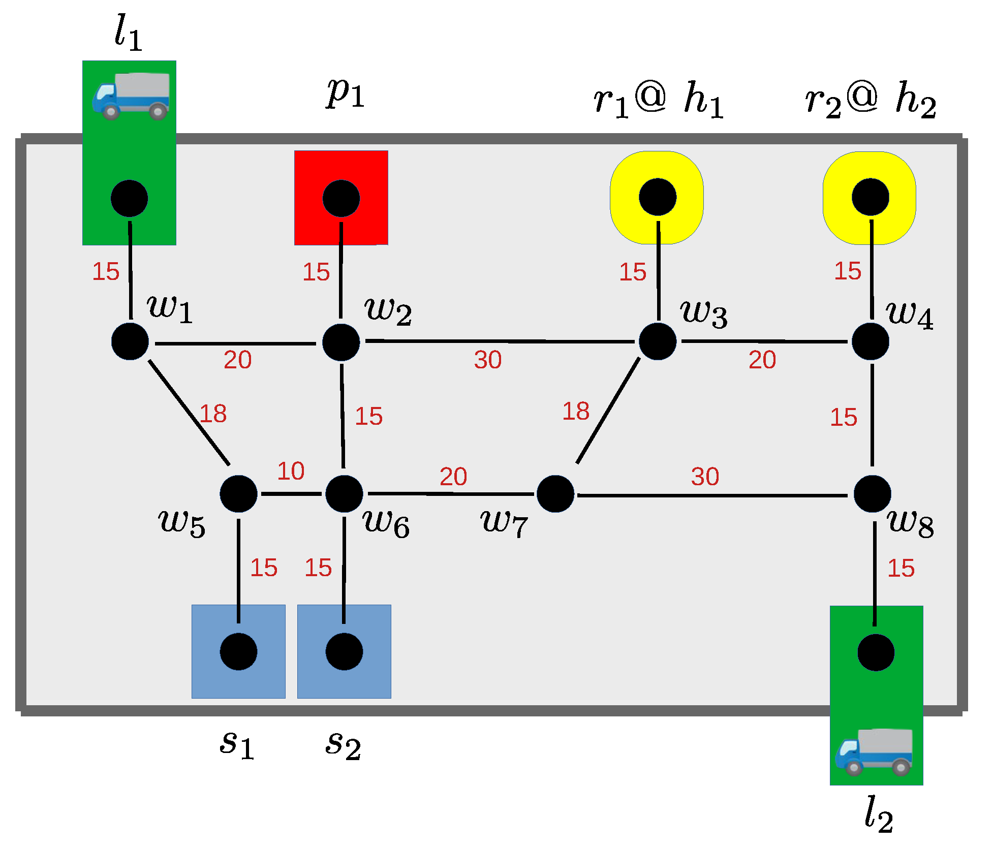
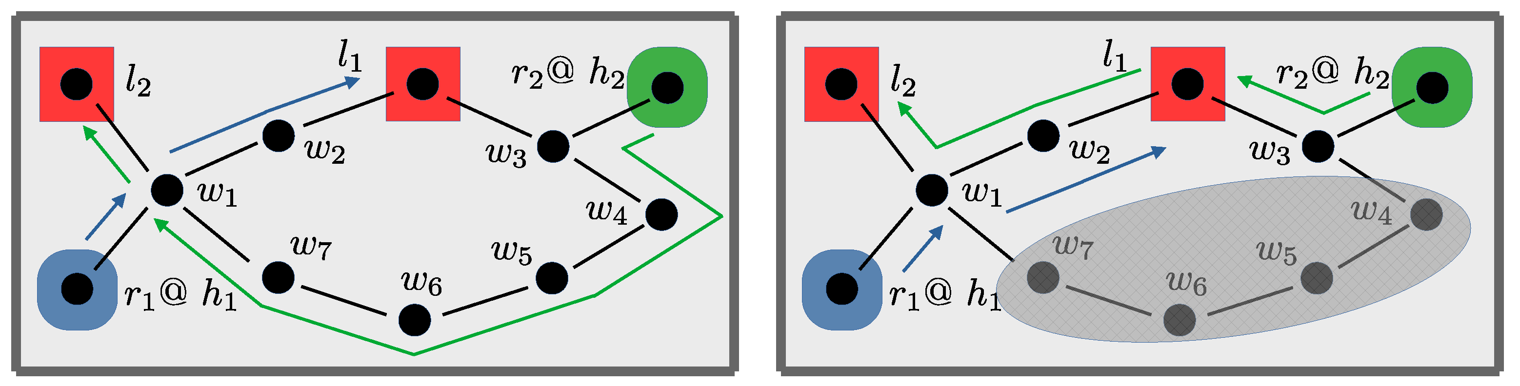
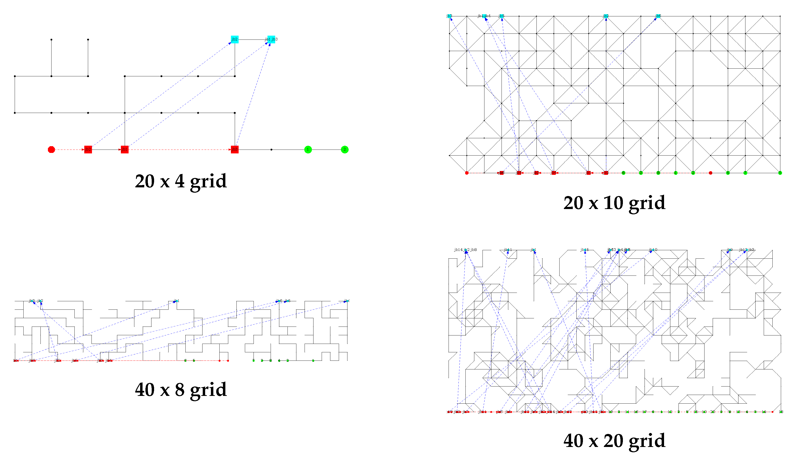
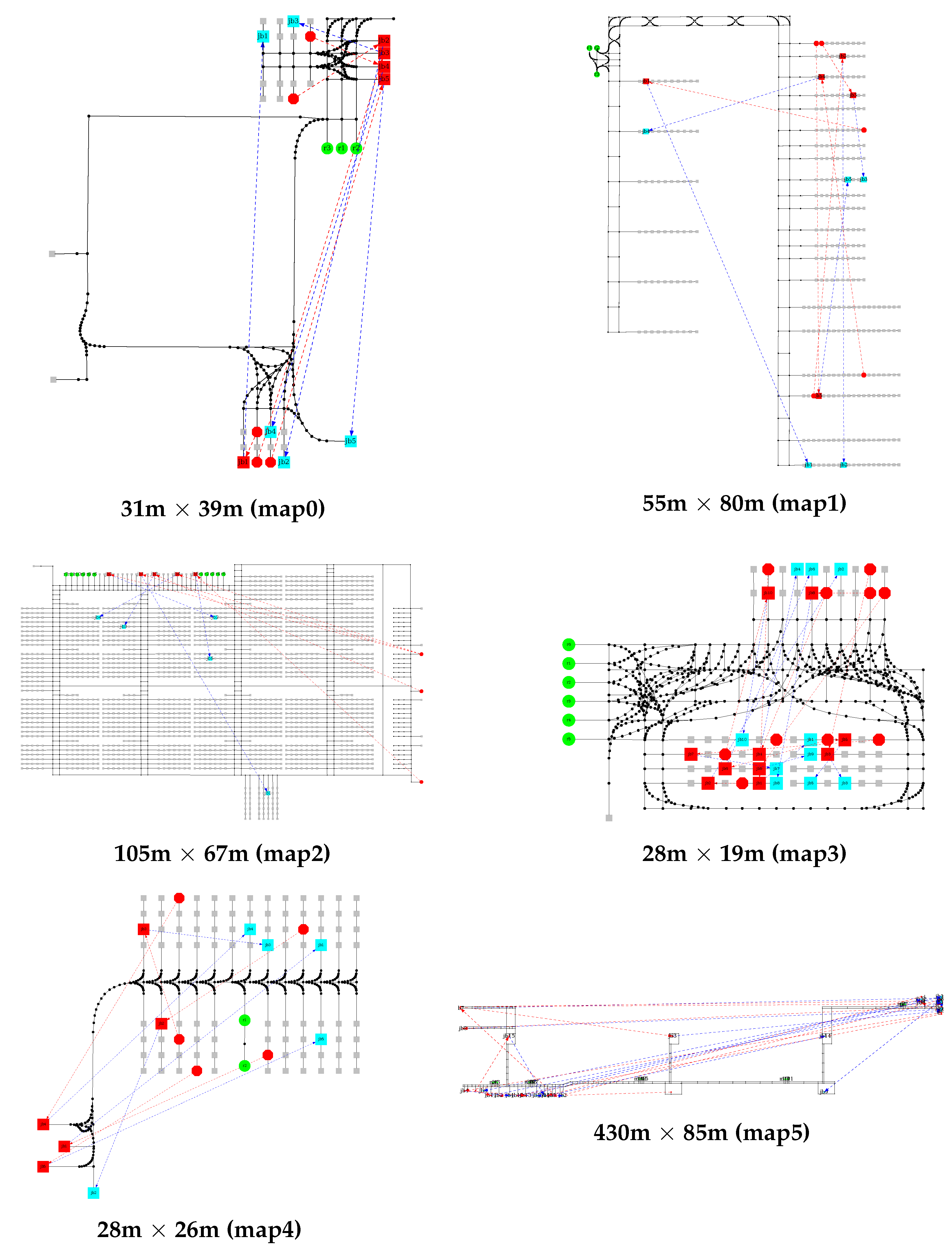
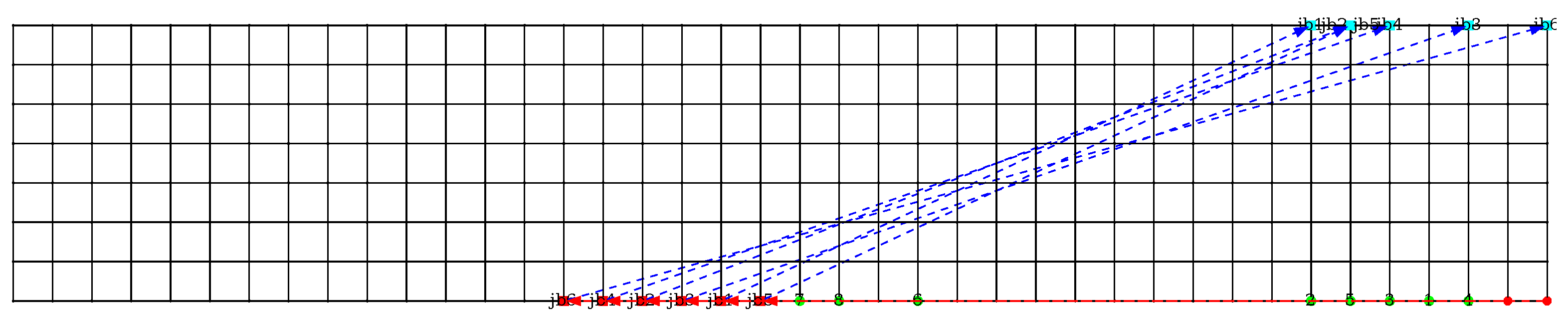4.6. Encoding Solution Quality

We accommodate both quality measures presented in Section 3.2. For measuring the makespan, we utilize the variable bound, as mentioned in Section 4.4.6. This allows us to either restrict the solution quality via a constraint of the form &diff{bound} <= q, where $q\in \mathbb{N}$ is the desired solution quality, or we can use clingo[dl]’s built-in branch-and-bound optimization by adding to the command line the option --minimize-variable=bound. Note that the latter method is computationally expensive and lacks clingo’s sophisticated optimization algorithms. This is the case because the scheduled values are not known to the solver and are stored in the background propagator handling difference constraints.

As for the task-pair distance, we assume an instance structure as in our running example. That is, every wait dependency expresses that something has to be retrieved from a loading bay before an empty pallet can be placed. Then, we only have to consider all tasks involved in such dependencies as our task pairs to accomplish that the task-pair distance expresses the maximum replacement time. Currently, we have no means of minimizing this measure, but we can restrict it to a certain value to enforce a desired solution quality. Listing 21 adds difference constraints to enforce the desired task-pair distance.

Listing 21. Add difference constraint representing an upper bound on the pallet replacement times.

1 #const replacement_bound=3*60*1000.   3 &diff{ arrive(T',V') - arrive(T,V) } <= replacement_bound :- 4           depends(wait,T,T'), task(T,V), task(T',V').

This pallet replacement bound provides a solution quality guarantee without resorting to computationally expensive optimization, as with makespan minimization. The constant replacement_bound should be overridden based on domain specific factors, such as the graph size and the expected ratio of tasks to robots.

5. Experiments

We evaluated our approach to the warehouse delivery problem using the Hybrid ASP system clingo[dl] v1.3.0, which is built on clingo v5.5.1. Given the industry focus of this work, the primary goal of these experiments is to understand the potential viability of our approach for solving real-world warehouse delivery problems. In particular, we evaluate the performance of the step-based and path-based encoding variants under different warehouse graph configurations and task loads.

While the focus is principally on the performant variants of the path-based encoding, the step-based encoding is also important to the evaluation. In particular, the step-base encoding provides a direct correspondence to the underlying problem formalization. In contrast, because the path-based encoding is restricted to acyclic paths, there are problem instances for which the step-based encoding admits a solution but the path-based encoding does not. Therefore the step-based encoding provides a baseline for our evaluation; both in terms of the solver performance but also to see whether the lack of completeness of the path-based encoding is an issue in practice.

We consider two sets of benchmarks. The first set of benchmarks consist of synthetically generated graphs, varying in size and graph density. The second set of benchmarks consist of real warehouse graphs, where we consider variations in the number of tasks and robots. The synthesized benchmarks have graphs with fewer vertices. On the other hand these benchmarks are grid-based in their construction, and in some cases are denser than the real warehouse graphs. Consequently, the differences in the two sets of benchmarks serve to highlight different performance features for a range of graph types and problem sizes.

For the real warehouse graphs we also consider a number of further variations to the problem instances. Firstly, we compare the performance when the size of each robot is treated as a single point versus when the robots are assigned non-point diameters of one and two meters. Importantly, depending on the graph vertex density, allowing for larger robots can result in an increase in the number of vertex conflict constraints. Secondly, we also consider how the addition of application specific constraints, in this case pallet replacement time constraints, affect solver performance. The pallet replacement constraints provide a mechanism to ensure good-enough plans without having to consider makespan minimization; which is computationally more expensive, and, as we shall see, ultimately impractical.

All benchmarks ran on a Linux computer with an Intel(R) Xeon(R) CPU E3-1260L v5 @ 2.90 GHz and 32 GB of RAM. Runs were given a memory limit of 30GB of RAM. For the experiments to find a single solution a time limit of 1800 s (30 min) was imposed. For the optimization runs with makespan minimization a longer time limit of 7200 s (2 h) was allowed. clingo[dl] was run in single-threaded mode, which ensures deterministic behavior and makes the experimental results repeatable. Finally, while we experimented with different solver configurations, clingo[dl]’s default tweety configuration provided good overall performance. In order to keep the presentation of the results manageable we only show the results for this default configuration.

5.1. Benchmarks

As mentioned earlier we consider two sets of benchmark problems to understand the performance limits of the different encodings and variants.

5.1.1. Crafted Benchmark

We generated a set of 50 problem instances of varying sizes and graph density. Graphs were generated from a number of grid configurations ranging in size from $20\times 4$ to $40\times 20$. For each size of grid the graphs were generated by varying the density of the vertices over the grid points and the connectedness between adjacent vertices. Each graph was also assigned a task execution graph consisting of between 2 and 20 robots and between 3 and 15 “jobs”. Note, we loosely use the term “job” here to describe two pairs of dependent tasks; so a single job consists of 4 distinct tasks. Each pair of tasks consists of a pickup and a putdown task; and the putdown of the second task pair has a wait dependency on the pickup of the first task pair. This corresponds to the industry scenario of a full pallet pickup-putdown from a loading bay to a storage location, as well as the corresponding pickup-putdown of a replacement empty pallet from the empty pallet storage to the newly vacated loading bay.

Figure 5 shows some example instances for a range of graph sizes. Note, the visualizations of benchmark graphs in Figure 5 and Figure 6 were generated using Clingraph [14], https://github.com/potassco/clingraph (accessed on 1 February 2023). The robots, pallet loading bays, and empty pallet storage locations were all placed on the south-most vertices, while the storage locations were placed on the north-most vertices. This ensured that each problem instance required routing over a substantial area of the graph.

5.1.2. Industry Benchmark

The industry benchmark consist of six distinct graphs handcrafted by domain experts at Dorabot, a provider of robotic and smart warehouse solutions. The graphs range in shape and size: 31 m × 39 m (map0), 55 m × 80 m (map1), 105 m × 67 m (map2), 28 m × 19 m (map3), 28 m × 26 m (map4), and 430 m × 85 m (map5). The graphs were provided in the OpenStreetMap (OSM) format, https://wiki.openstreetmap.org/wiki/OSM_XML (accessed on 1 February 2022), which we converted to our ASP graph fact format by converting the OSM edges to weighted edge/3 facts while assuming a constant velocity of 1 m/s. For example, an OSM edge that is 1.5 m in length is converted to an edge/3 fact with a weight of 1.5 s (which we represent as 1500 ms to remove the need for floating point numbers).

For each graph the allowable loading bay, storage, empty pallet, and robot home vertices were indicated with OSM attributes. In order to support more robots, we added some graph variants that increased the number of robots by turning some unused storage vertices into robot home locations. The maximum allowable robot home vertices for each graph ranged from 2 to 20 robots. For each map-robot configuration we then generated instances (5 instances each) with differing number of jobs from 5 to 40 depending on the capacity of the graph. As previously described, each job consists of two pairs of dependant tasks that constitute a full pallet delivery and its corresponding replacement empty pallet delivery. The maximum job capacity for each graph varied, with one graph only supporting 15 jobs (60 distinct tasks), some supporting 20 jobs (80 distinct tasks), others supporting 30 jobs (120 distinct tasks), and finally two supporting 40 jobs (160 distinct tasks). Overall this produced 215 distinct problems instances. See Figure 6 for an example instance from each of the warehouse graphs.

Note, that at the maximum number of task and robots some of the generated problem instances are potentially larger than what might be required in a real-world setting. However, our intention in generating this wide range of problem instances, from those with a relative few number of tasks to those with a large number of tasks, has been to explore the performance limits of our encodings.

5.2. Encodings Variants

In this sub-section we outline the different encoding variants used for the experiments. While some variants apply to both the step-based and path-based encodings, the majority of variants rely on pre-computed shortest path information and therefore only apply to the path-based encoding. Finally, we also consider the application specific variant of adding pallet replacement time constraints, which we also only apply to the path-based encoding for solving the industry benchmarks.

5.2.1. Basic and Task Acyclicity Variants

For the step-based and path-based encodings we tested the basic encodings as well as the variants with added task acyclicity checking. To be clear, all variants produce correct solutions but the basic variants have no enhancements to improve performance.

Both the step-based and path-based encodings support the addition of task sequence acyclicity checking, using the #edge directive, shown in Listing 4. Additionally, we also added the acyclicity check of Listing 5 to enforce task wait dependencies. As outlined in Section 4.2 the task acyclicity check can also be encoded in pure ASP using a reachability encoding (Listing 3). However, in all our experiments the reachability version for detecting task acyclicity under-performed the #edge variant, so we do not report on these results here. In our results tables we use the abbreviation TskAcyc(W) to indicate the use of task acycyclicity checking with wait dependencies.

5.2.2. Shortest-Path Enhancements

As the path-based encoding treats the notion of a path as a primitive, this enables many performance enhancements based on using pre-calculated shortest path information (see Section 4.5). For each problem instance, the shortest path information was pre-calculated using the FloydWarshal algorithm [15]. For a fast Python implementation of FloydWarshal see https://gist.github.com/mosco/11178777 (accessed on 1 February 2022). Note, here we calculated the shortest path information separately for each problem instance. However, in a production environment this information would typically to be calculated only once for each warehouse graph, and then filtered based on the particular tasks that make up the problem instance.

Lower-Bound Propagation

The first use of the shortest-path information that we evaluated was for propagating path length lower-bounds (Listing 17). We use the abbreviation LB  to indicate the use of lower-bound propagation in a configuration. Because lower-bound propagation showed only positive performance results we used it as the basis for all subsequent configurations.

Corridor Restrictions

To foreshadow the presentation of results, the path-based encoding can ground many more problem instances that are simply beyond the reach of the step-based encoding. Nevertheless grounding was still problematic for the path-based encoding when the paths were unconstrained. In order to reduce the grounding we restricted the allowable moves of the robots to a corridor constructed around the shortest-path information, as shown in Listings 19 and 20. We considered both the strict and non-strict corridor definitions, where the non-strict version simply drops the N’ <= N restriction to the rules in Listing 19. For the strict corridor definition we use the abbreviation Corr(S) and for the non-strict version we use the abbreviation Corr(NS). We consider both versions because there are some few cases where the strict definition makes the problem harder to solve without additional performance enhancements.

Domain Heuristics for Moves

Unarguably, the most important performance enhancement we consider is the addition of the domain heuristics for selecting moves. The main move heuristic we consider is the negative heuristic of preferring to set moves that are not on a shortest path to false. This is encoded in the rule at Line 7 of Listing 18. We use the abbreviation MvH  to indicate the use of this heuristic.

While the negative move heuristic always improved solver performance, we also considered the case where this heuristic is supplemented with the additional heuristic of weakly preferring moves that are on a shortest path. This weak preference heuristic is encoded in the rules at Lines 1 and 4 of Listing 18, and we use the abbreviation MvH(P) to indicate its use.

5.2.3. Move Routing Acyclicity Checking

As discussed in Section 4.4.4 the time-based path acyclicity checking of the base routing rules (Listing 11) can be supplemented by the addition of explicit acyclicity checking of the moves along a path. We considered both the pure ASP encoding using reachability (Listing 12) and using the edge/3 encoding (Listing 13). For the pure ASP reachability encoding we use the abbreviation MvR  and for the edge/3 based encoding we use the abbreviation MvA. We report on the performance of these two additional move acyclicity checkers separately as well as working together.

5.2.4. Pallet Replacement Time Bound

Finally, we report on the use of the pallet replacement time bound as a mechanism for providing a quality guarantee that can be computed quickly while providing a good-enough solution. Because determining an appropriate pallet replacement time bound is specific to a specific warehouse and problem configuration we do not perform these experiments on the synthetically generated graphs of the crafted benchmark, and only perform these experiments for the warehouse graphs of the industry benchmark. For most of the warehouse graphs we considered a pallet replacement time bound of 300 s and 400 s, however for the largest warehouse (map5) we used a bound of 800 s because some instances were simply not satisfiable given the lower bounds.

5.2.5. A Note on Step Encoding Horizons

The step-based encoding requires a horizon value that fixes the maximum length of any robot walk. A balance needs to be found between a horizon that is large enough to admit solutions and a horizon that is not so large that the problem instance fails to ground.

Since the size of the ground instance is directly correlated with the horizon, and we conjectured that grounding would be a major hurdle for the step-based encoding, ideally we would want to use the smallest horizon possible for each problem instance. However, determining this value for each problem instance would have been impractical, potentially needing to run each problem instance 100 s or 1000 s of times with varying horizon values to find this minimum value.

As a compromise we used the results generated by the solution of the path-based encoding. While the path-based encoding does not require a walk horizon, a horizon value can be calculated from each solution, using the translation described in Section 4.4.7. To approximate the minimum horizon we used the horizon value calculated when minimizing the makespan for the path-based encoding (with a 2 h time limit).

Note, there are two caveats to this approach. Firstly, most problem instances timed out after 2 h so the makespans found were not necessarily minimal. Secondly, the horizon value calculated from a minimal makespan solution does not guarantee that the horizon itself will be minimal. A solution with a minimal makespan solves the problem in the shortest amount of time, but this does not guarantee that the maximum number of steps required for all robots is also minimal. Nevertheless the two are loosely correlated so such a solution will provide a horizon that is close to the minimal.

Unfortunately, as we shall see in the next section (Section 5.3), despite our best efforts most problem instances simply failed to ground. While it is conceivable that there could be some cases where our approximation of the horizon was not good enough, however, considering that even for the basic path-based encoding there where 55 instances that failed to ground, finding a better horizon for just a few more instances of the step-based encoding would always be of limited use. Some form of restriction to reduce the grounding, such as the move corridors used in the path-based encoding, would still be required. Importantly, such corridor restrictions are difficult to define for the step-based encoding because there is no primitive path concept on which to anchor such a definition.

5.3. Results

We now report on our experimental results. To establish the base-line and to highlight the dramatic improvements of the path-based encoding with performance enhancements, we first compare the step-based encoding with both the basic and most performant path-based encodings. Here we only looked at the basic problem of finding a single solution to see which encoding variant could find a solution within the 30 min time limit.

Having established a base-line with the step-based encoding, we next focus entirely on the path-based encoding highlighting features of the different encoding variants. This identifies the most performant path-based encoding variant, Path + LB + Corr(S) + TskAcyc(W) + MvA + MvR + MVH, which we use for the remaining experiments. To better understand the limits of the path-based encoding on the industry benchmark we separate the instances by the graph and number of jobs. Then we look at the impact of the performance of solving on the size of the robot, comparing a point sized robot against one meter and two meter diameter robots. Finally, we consider solution quality. Here we consider the addition of the pallet replacement time constraints and compare the solving time and resulting makespan metric against solving to find the minimal makespan.

5.3.1. From Step Encoding to Best Path-Base Encoding Variant

Table 4. Comparison of the step encoding and path encodings, from basic to most performant variants. Note, means and geometric means of runtimes apply to grounded instances only.

Configuration	Benchmark	SAT/ UNSAT/ UNKNWN	Time Out	Mem Out	Runtime Mean/Geo.Mean (Excl. Mem Out)
Step Basic	Crafted	10/2/38	4	34	43.46/472.92
	Industry	0/0/215	0	215	-/-
	Total	10/2/253	4	249	43.46/472.92
Step TskAcyc(W)	Crafted	10/2/38	4	34	45.36/474.61
	Industry	0/0/215	0	215	-/-
	Total	10/2/253	4	249	45.36/474.61
Path Basic	Crafted	35/2/13	13	0	20.48/527.56
	Industry	0/0/215	169	46	1800.00/1800.00
	Total	35/2/228	182	46	647.81/1509.49
Path + LB + Corr(NS)	Crafted	37/2/11	11	0	6.88/400.84
	Industry	100/0/115	115	0	338.08/1069.35
	Total	137/2/126	126	0	162.12/943.22
Path + LB + Corr(S)	Crafted	48/2/0	0	0	1.07/5.13
+ TskAcyc(W)	Industry	209/0/6	6	0	22.41/124.47
+ MvA + MvR + MvH	Total	257/2/6	6	0	12.63/101.95

compares the step-based encoding, with and without task acyclicity checking, against a selection of path-based encoding variants. For the path-based encoding we highlight the basic variant, a variant with a corridor restriction, and finally, a variant with the most performant enhancements. These results serve to highlight the full range of behaviors for the different encodings and their variants.

Firstly, we can see that while the step-based encoding can solve some of the crafted problem instances it failed on all of the industrial problem instances. For all of the industry benchmark, and most of the crafted benchmark instances, clingo[dl]  simply ran out of memory and failed to ground the problem.

Note, as we used the #edge-based task acyclicity checking for the high-performant path-based encoding, and because it was the only performance enhancement that we consider for the step-based encoding, we therefore also compare this variant of the step-based encoding with the basic variant. However, as we can see in Table 4 there is no benefit of adding task acyclicity checking for the step-based encoding.

Besides the fact that the step-based encoding failed to ground most problem instances, there are two points to highlight. Firstly, while the basic path-based encoding was able to ground many more instances than the step-based encoding, nevertheless it still failed to ground a significant number of the industrial problems. However, when we added a corridor restriction it was able to ground all of the problem instances. Furthermore, with the corridor restriction, and lower-bound propagation, it also reduced the number of time outs and allowed many more additional problem instances to be solved. The final point to highlight is to do with the performance of the best variant of the path-based encoding, Path + LB + Corr(S) + TskAcyc(W) + MvA + MvR + MVH. Not only did it ground all problem instances, but it was also able to solve most of them; in some cases in a matter of seconds and in other cases within a few minutes.

Note, the mean and geometric means for runtimes apply only to the grounded problem instances. Consequently, the reason that the runtimes for the basic path-based encoding are higher than the basic step-based encoding is simply that the step-based encoding was not able to ground the hard problem instances. The basic path-based encoding grounded a majority of these instances, even though it subsequently failed to solve them within the time limit.

5.3.2. Comparison of Path-Based Encoding Variants

Table 5. Comparison of path encoding variants with/without basic move heuristic and differing in move corridor types and task/move acyclicity checks. Note, all problem instances grounded successfully so we only report on whether the problem was solvable or whether it timed out.

Configuration	Benchmark	Solved	Time Out	Runtime Mean/Geo.Mean
Path + LB + Corr(NS)	Crafted	39	11	6.88/400.84
	Industry	100	115	338.08/1069.35
	Total	139	126	162.12/943.22
Path + LB + Corr(S)	Crafted	43	7	3.20/265.02
	Industry	138	77	79.12/704.28
	Total	181	84	43.20/621.40
Path + LB + Corr(NS)	Crafted	50	0	1.37/5.34
+ MvH	Industry	209	6	32.43/171.51
	Total	259	6	17.86/140.16
Path + LB + Corr(S)	Crafted	49	1	1.21/39.59
+ MvH	Industry	207	8	24.79/148.78
	Total	256	9	14.03/128.18
Path + LB + Corr(NS)	Crafted	50	0	1.30/13.94
+ MvH + TskAcyc(W)	Industry	210	5	30.67/154.98
	Total	260	5	16.90/128.37
Path + LB + Corr(S)	Crafted	49	1	1.16/38.85
+ MvH + TskAcyc(W)	Industry	210	5	22.05/116.99
	Total	259	6	12.65/102.25
Path + LB + Corr(S)	Crafted	49	1	1.17/38.75
+ MvH + TskAcyc(W)	Industry	210	5	21.58/114.00
+ MvA	Total	259	6	12.44/99.80
Path + LB + Corr(S)	Crafted	50	0	1.10/26.06
+ MvH + TskAcyc(W)	Industry	210	5	22.50/128.37
+ MvR	Total	260	5	12.74/109.07
Path + LB + Corr(NS)	Crafted	50	0	1.40/6.40
+ MvH + TskAcyc(W)	Industry	210	5	30.93/141.50
+ MvA + MvR	Total	260	5	17.25/116.01
Path + LB + Corr(S)	Crafted	50	0	1.07/5.13
+ MvH + TskAcyc(W)	Industry	209	6	22.41/124.47
+ MvA + MvR	Total	259	6	12.63/101.95

compares variants of the path-based encoding with a view to identifying the variant with the best overall performance. We only consider variants with some form of move corridor restriction, since Table 4 shows that variants without a move corridor had many problem instances that failed to ground. As these configurations were able to ground all problem instances, therefore, on top of the runtime results, we only report the number of problem instances that were solved versus the number that timed out.

There are a number of interesting behaviors that can be observed from these results. Firstly, the most dramatic improvement in performance comes from the use of the basic move heuristic, where the move heuristic sets move/3 facts that are not on the shortest path to false. Without the move heuristic the number of timeouts was 126 and 84 for the non-strict and strict move corridors, respectively. This dropped dramatically to 6 and 9, respectively, with the addition of the move heuristic.

The second interesting behavior comes from the difference between the strict and non-strict move corridors. Using the strict corridor over the non-strict corridor typically improves solver performance for most cases, but results in timeouts for a few cases. Adding task acyclicity detection and move acyclicity detection with a reachability encoding was able to solve more cases. Interestingly for the crafted benchmark adding the move acyclicity reachability encoding allowed the one problematic instance to be solved. This is a particularly interesting case, because, unlike the industry benchmark problems which are large in size, the crafted problems are relatively small. Consequently it is useful to examine this problematic instance (Figure 7) in more detail to understand the difference between the strict and non-strict corridor versions.

The densely connected grid structure, meant that the strict corridor definition, which requires that corridor vertices be no further from the goal vertex than a shortest path vertex, failed to define an adequate corridor beyond the shortest paths themselves. Furthermore, there was significant clustering for the task source vertices and task destination vertices. The combination of this clustering and the pure shortest path corridors resulted in the search for a conflict free route for each task’s path being dominated by the potential vertex conflicts. Without the explicit task and move acyclicity checking, this resulted in a heavy burden on the difference logic solver to resolve the very fine grained timing required to avoid conflicts.

In contrast the non-strict corridor allows all vertices connected to a shortest path vertex to be part of the corridor, so in this case a wider corridor could be generated. This in turn provides greater flexibility in the allowable moves of the robots in order to avoid conflicts, and less heavy lifting is required by the difference logic solver.

The final observation from Table 5 is that there is no clear winner between the top path-based encoding variants with #edge-based task ayclicity checking and both #edge-based and reachability based move acyclicity detection. Using a non-strict corridor definition does allow more instances to be solved, in this case a single instance, but increases the solver runtime. The best choice of performance enhancements for a given scenario will therefore depend on the specific warehouse graph. For the sake of this paper, we have chosen the strict corridor version as our candidate winner. It had marginally, but also consistently, better runtimes than the best non-strict corridor based encoding for both the crafted and industry benchmarks.

5.3.3. Comparison of Move Heuristics

As discussed in Section “Domain Heuristics for Moves” we consider two variants of the move heuristic. The first move heuristic we consider preferences setting moves that are not on the shortest-path to false. However, this heuristic does not specify any additional heuristic behavior for moves that are on the shortest path. The second heuristic extends the first heuristic by enforcing a weak preference for setting moves on the shortest-path to true. Results of these two variants for a number of configurations are shown in

Table 6. Comparison of path encoding configurations for two variants of the move heuristics.

Configuration	Benchmark	Solved	Time Out	Runtime Mean/Geo.Mean
Path + LB + Corr(S)	Crafted	49	1	1.21/39.59
+ MvH	Industry	207	8	24.79/148.78
	Total	256	9	14.03/128.18
Path + LB + Corr(S)	Crafted	49	1	1.19/39.45
+ MvH(P)	Industry	208	7	24.40/154.62
	Total	257	8	13.81/132.89
Path + LB + Corr(S)	Crafted	49	1	1.16/38.85
+ MvH + TskAcyc(W)	Industry	210	5	22.05/116.99
	Total	259	6	12.65/102.25
Path + LB + Corr(S)	Crafted	49	1	1.13/38.62
+ MvH(P) + TskAcyc(W)	Industry	210	5	22.62/128.49
	Total	259	6	12.86/111.54
Path + LB + Corr(S)	Crafted	49	1	1.17/38.75
+ MvH + TskAcyc(W)	Industry	210	5	21.58/114.00
+ MvA	Total	259	6	12.44/99.80
Path + LB + Corr(S)	Crafted	49	1	1.13/38.23
+ MvH(P) + TskAcyc(W)	Industry	210	5	21.97/122.41
+ MvA	Total	259	6	12.56/106.52

.

For each configuration there was only margin differences in performance between the MvH and MvH(P) variants. However, in all cases the simpler MvH variant performed slightly better. Consequently, for all remaining experiments we only report on the MvH results.

5.3.4. Runtime with Increasing Number of Tasks

Table 7. Comparison of runtimes and makespans by map and and number of tasks for the high performance path encoding variant Path + LB + Corr(S) + TskAcyc(W) + MvA + MvR + MVH.

Map	Num Robots	Num Jobs (4 Tasks per Job)	Time Out	Makespan (seconds) Mean/Geo.Mean	Runtime Mean/Geo.Mean
map0	4	5	0	352/363	1.20/1.20
		10	0	842/855	6.00/6.05
		15	0	1308/1311	16.24/16.42
map1	3	5	0	1184/1198	2.33/2.33
		10	0	2554/2581	10.38/10.42
		15	0	3331/3343	28.32/28.45
		20	0	4805/4830	71.32/72.55
		30	0	6779/6848	308.39/327.74
		40	0	8790/8805	797.99/852.29
map2	11	5	0	1038/1052	6.52/6.53
		10	0	2450/2463	25.63/26.03
		15	0	3870/3873	84.45/85.26
		20	0	4808/4814	232.87/242.04
		30	1	7322/7343	973.34/1059.79
		40	5	-/-	1800.00/1800.00
map3	7	5	0	301/308	2.12/2.13
		10	0	573/580	7.90/7.92
		15	0	1045/1050	23.44/23.61
		20	0	1361/1371	51.77/52.46
		30	0	2321/2342	222.00/227.06
map4	2	5	0	341/354	1.11/1.12
		10	0	656/662	5.16/5.18
		15	0	926/934	15.68/15.78
		20	0	1228/1236	39.64/40.35
map5	20	5	0	3520/3561	11.25/11.26
		10	0	8008/8079	30.52/32.35
		15	0	13,467/13,517	121.64/138.78
		20	0	18,469/18,537	617.26/734.76

highlights the scalability of the encoding as the number of tasks increases for each graph. As expected the runtime increases as the number of tasks increase. For each of the six graphs, solving for 10 jobs (i.e., 40 tasks) was relatively easy, with a maximum geometric mean of 32.35 s for the largest map (map5). For context the geometric mean of the makespans in this case was 8079 s; so it took approximately 30 s to generate a plan for more than 2 h of robot operations. In this case the warehouse is very large (480 m × 85 m) so the plans typically span relatively long distances for the robots to complete their tasks.

If we hypothetically consider a maximum runtime of 60–90 s as an expectation for operating in a semi-realtime environment, then for most of the graphs the solver could comfortably plan for up for 20 jobs. The two exceptions to this being the two biggest graphs, map2  and map5. map5  could only solve for 10 jobs before breaching this limit, while map2  could solve for 15 jobs, the latter generating solutions with a 3873 s makespan (approx. 1 h). Unfortunately, for map2  the solver could not solve any instances containing 40 jobs within the 30 minute time limit.

5.3.5. Runtime with Differing Robot Diameters

Table 8. Comparison of solving for a point-sized robot vs. a circular one and two meter diameter robot, for the high performance path encoding variant Path + LB + Corr(S) + TskAcyc(W) + MvA + MvR + MVH.

Map	Robot Diamater	Time Out	Mem Out	Runtime Mean/Geo.Mean (Excl. Mem Out)
map0	Point size	0	0	4.89/7.89
(15 instances)	One meter	0	0	24.46/52.26
	Two meter	0	0	64.53/141.11
map1	Point size	0	0	47.87/215.63
(30 instances)	One meter	0	5	117.45/333.81
	Two meter	0	10	166.70/289.34
map2	Point size	6	0	133.88/536.63
(30 instances)	One meter	6	0	133.51/535.30
	Two meter	4	10	302.63/576.09
map3	Point size	0	0	21.42/62.63
(25 instances)	One meter	2	0	101.35/405.24
	Two meter	4	5	264.22/591.31
map4	Point size	0	0	7.72/15.61
(20 instances)	One meter	0	0	78.78/249.63
	Two meter	0	6	125.92/239.33
map5	Point size	0	0	71.26/229.29
(20 instances)	One meter	0	0	65.40/180.52
	Two meter	5	0	314.24/684.35

shows the effect of the diameter of the robot on solver performance. In Listing 14, Lines 5 to 13, the encoding generates conflict constraints for pairs of paths and vertices that can potentially interfere with each other. This is one of the main sources of combinatorics for the encoding. Consequently, as the size of each robot increases, the number of vertex conflicts will also increase, and will result in an increase in the number of conflict constraints. This in turn increases in the size of the ground program. One would also expect an increase in the solver runtime as these additional constraints need to be resolved.

Because of the variation in the vertex densities of the different maps it is worth looking at these result separately for the individual maps. Table 8 shows that as the diameter of the robots increase we start to see problems as more and more instances fail to ground. Furthermore, as expected, the solver runtimes increase with timeouts becoming more frequent. Note, in Table 8 the runtime results only apply to problem instances that were able to be grounded. So the reason that the runtimes may not increase as much as expected can simply be a result of the harder problems failing to ground and therefore not being included in the aggregate solver runtime values.

These results highlight the importance of choosing the correct level of granularity for a warehouse graph. A balance needs to be found between the need to plan high-level robot tasks and plan relatively low-level movements that might be better handled by a low-level robot motion controller. For example, while map3 (Figure 6) is relatively small in size it has a very dense set of vertices. While this allows for fine-grained path planning for the robots, it also results in large clusters of conflicting vertices that need to be resolved.

Finally, while reducing the density of vertices in the graph is one possibility for dealing with an increase in conflicting vertices, a second option would be to separate the conflict handling from the path routing. In particular, it would be possible to group vertices into larger blocks where conflict handling is performed on the blocks rather than on the individual vertices. We discuss this possibility further in Section 7.

5.3.6. Solution Quality with Pallet Replacement Time Bounds

To this point in the experimental results we have been primarily interested in solver runtimes; identifying the path-based encoding variant Path + LB + Corr(S) + TskAcyc(W) + MvA + MvR + MVH that solves the greatest number of benchmark instances in the shortest amount of time. In this section, we use this encoding variant but turn to examining the question of solution quality.

Table 9. Comparison of makespan by map and decision problem for the high performance path encoding variant Path + LB + Corr(S) + TskAcyc(W) + MvA + MvR + MVH.

Map	Decision Problem	Time Out	Makespan (seconds) Mean/Geo.Mean	Runtime Mean/Geo.Mean
map0	Minimal	30	345/422	7200.00/7200.00
(30 instances)	Pallet Rpl. 200 s	0	653/734	5.60/10.15
	First Soln	0	771/896	4.82/7.88
map1	Minimal	50	1891/2734	7200.00/7200.00
(50 instances)	Pallet Rpl. 400 s	5	2443/2884	49.60/325.60
	First Soln	0	3241/3919	28.84/136.39
map2	Minimal	50	1660/2627	7200.00/7200.00
(50 instances)	Pallet Rpl. 200 s	6	2060/2333	87.70/354.24
	First Soln	6	3007/3545	60.85/278.82
map3	Minimal	45	413/575	7200.00/7200.00
(45 instances)	Pallet Rpl. 200 s	0	665/789	20.38/106.45
	First Soln	0	810/1009	15.51/40.97
map4	Minimal	20	412/481	7200.00/7200.00
(20 instances)	Pallet Rpl. 200 s	0	611/695	12.69/40.73
	First Soln	0	716/804	7.83/15.73
map5	Minimal	20	4916/6876	7200.00/7200.00
(20 instances)	Pallet Rpl. 800 s	8	6206/6958	446.19/1078.63
	First Soln	0	9064/10,747	64.60/180.25

compares the makespan produced for computing a single solution with, and without, a given pallet replacement time constraint, and compares this to searching for the minimal makespan. The pallet replacement time is an application domain criteria and is highly sensitive to the specific warehouse graph. Therefore it only makes sense to evaluate this criteria with respect to the industry benchmarks consisting of real-world warehouse graphs, rather than the crafted benchmarks consisting of synthesized graphs. Note also, from Table 4, we know that the industry benchmarks consist of only satisfiable problem instances, which of course is a necessity for measuring solution quality.

There are a number of points to highlight here. Firstly, searching for a provably optimal solution is unrealistic in a practical setting. In our evaluation, searching for the optimal solution failed to prove optimality, within the 7200 s (2 h) timeout, for every problem instance. In contrast finding a single solution took between a few seconds and a few minutes. Note, for clarity it is worth pointing out that finding an optimal solution and proving that that solution is indeed optimal are separate things. Once a solution is found the solver still needs to ensure that there are no better solutions, so it is possible to find an optimal solution within the time limit but not prove its optimality.

It should also be pointed out that when returning the first solution, the makespan was typically around twice that of the makespan found for the optimality search, which in itself could be considered a good enough solution under some application settings. A primary reason for this relatively good solution quality is to do with the move heuristic and the difference logic solver. The move heuristic ensures that the paths are close to the shortest possible, while the algorithm for the difference logic solver returns the lowest possible integer value for each variable, which effectively minimizes any time delays on a given path. This means that any robot’s moves along a path will always be close to optimal. So it is only within the allocation and ordering of tasks, and not the moves themselves, that the main improvements in makespan can be made.

When the pallet replacement time constraints were added, the solving time for finding the first solution increased by up to a factor of 3. So for example, with map0  the geometric mean of the runtimes increased from 7.88 to 10.15 s, while for map4  it increased from 15.73 to 40.73 s. It should also be observed that enforcing the pallet replacement time bound also improved the makespan. The makespan often improved significantly, roughly halving the difference between the first and best solutions.

Finally, whether or not the pallet replacement time metric provides good-enough solutions will depend on the requirements of the given warehouse application. There are also further possibilities that could be explored in the future to determine a good-enough criteria for a given application. For example, when optimization is enabled, the solver returns the solutions as they are found. This allows the solver to be used in an anytime setting, returning the best solution up to some fixed timeout. So it could be interesting to compare the quality of the solutions for makespan minimimization as they are produced over time. It could be the case that the search gets close to an optimal solution quite quickly, even if it is ultimately not practical to wait for the provably optimal solution to be found.

6. Related Work

The warehouse delivery problem considered in this paper can be viewed as a specialized instance of the multi-agent path finding (MAPF) problem that has attracted a lot of attention in recent years due to its widespread applicability. Introductory materials on MAPF can be found in the papers [12,16] and several tutorials at AAAI, IJCAI, or ICAPS. Challenges and opportunities in MAPF and its extensions have been described by [17]. The present paper considers weighted graphs and robots that have a size that can place complex constraints on possible movements, e.g., a robot can block more than one vertex at a time and travel time between vertices is different.

As MAPF is essentially a planning problem, search-based approaches to solving MAPF are frequently used. Indeed, a plethora of MAPF solvers have been proposed [18,19,20,21,22,23,24,25,26,27]. They can be classified into different groups based on their search techniques such as conflict-based search (CBS) or prioritized planning (PBS)) or the solution quality such as optimal, bounded-optimal, or suboptimal solutions of MAPF.

Conflict-Based Search (CBS) is proposed in [21]. In this approach, the high-level search identifies constraints between plans of agents generated by a low-level $A^{*}$ search. These conflicts are then resolved using the low-level searches for new plans for a subset of conflicted agents. CBSH2-RTC [19] is the state-of-the-art version of CBS and is well known for its performance compared to other optimal MAPF solvers.

Enhanced CBS (EBCS)  [28] relaxes the optimal criteria in CBS and returns suboptimal solutions whose costs are bounded by some user-defined factor by replacing the optimal search in different levels of CBS with focal search that uses an admissible heuristic for bounding the solution cost at the higher-level and another heuristic in guiding the search. EECBS [27] is an improved version of EBCS by replacing the high-level search in ECBS with Explicit Estimation Search [29] and uses online learning to guide the search.

PBS [30] is a suboptimal MAPF solver that uses the idea of prioritized planning [31]. In this approach, agents are assigned different priorities and those with lower priority need to avoid having any conflict with higher-priority agents. PBS adopts a lazy exploration method that allows it to considers a total priority orderings. PBS is not complete solver.

In recent years, several extensions of the MAPF problem have been introduced. These extensions focus on the assumptions made in the classical MAPF. For example, combined Target Assignment and Path Finding (TAPF), where agents are partitioned into teams and each team is given a set of targets that they need to reach, is considered in [32]. Deadlines of tasks are addressed in [33]. MAPF problem with delay probabilities have been described by [34]. Lifelong MAPF is considered in [35]. The paper [36] investigates MAPF with continuous time, which removes the assumption that transitions between nodes are uniform. A SAT-based solver described in the paper [37] can also deal with this extension. SMT-based MAPF solver for MAPF with continuous time and geometric agents is described in [38]. Issue of unexpected delays of agents is considered in [39]. This paper introduces the notion of k-robust MAPF plan, which can still be successfully executed when at most k delays happen and investigate $pk$-robots MAPF plan, a probabilistic extension of k-robust MAPF plan. A somewhat more realistic version of MAPF, which allows agents to exchange packages and transfer payload, is considered by [40]. Discussion of the problems where robots have kinematic constraints can be found in the paper [41].

As we have mentioned above, the present paper addresses two assumptions in the classical MAPF problem, the disregard for robot size and the equal-distance between neighbors. Among these extensions, our work has some similarity to the multi- agent pickup and delivery (MAPD) problem, introduced in [35], in which one agent might have to complete many pickup-then-delivery tasks in an online setting. The warehouse delivery problem considered in this paper requires each robot completes at most one pickup-then-delivery task. Its natural extension will be the MAPD problem and we leave it for the future.

The present paper provides an ASP-based approach to solving an extension of MAPF problem and therefore is strongly related to ASP-based encodings proposed in [42,43,44,45]. Among these works, reference [42] considers the classical MAPF, while reference [45] solves the sum-of-cost variant of MAPF, and [43,44] tackles a more generalized MAPF problem. None of these works, however, consider robots with sizes that can block multiple vertices or graphs with non-uniform distances between vertices as in this paper.

The paper [43] discussed the MAPF problem in the context of a warehouse with picking stations, shelfs, orders, and quantities. It introduced the asprilo framework for experimental studies of MAPF problems, and thus, presented several scenarios and step-based encodings. These encodings, however, cannot deal with weighted graph (grid) or robots of different sizes. Experimental evaluation of various encodings was presented but for rather short makespan (≤40) that is well below the need of problems considered in this paper.

The paper [45] exploited a step-based encoding of MAPF and described different improvements to the generic encoding that helps reducing the size of the grounding of a problem. It also utilized parallel plans and used clingo with multiple threads to compute solutions. Similar to [43], the experiments shown in this paper implies a much smaller size of maps that does not meet the need of our applications.

The paper [44] employed an approach to solving TAPF problems. Focusing on the warehouse problem, the approach consists of three steps. First, it creates a simplified graph by combining nodes together. Second, it solves the problem on the simplified map. Third, it uses the solution in the second step as the skeleton to compute the final solution. This allows for the system to scale up quite well, being able to solve problems with more than 1,5 millions nodes. In our view, the path-based encoding of the present paper is similar in the spirit of this approach as it attempts to first creates multiple segments of the solution and then combining them to get the final solution.

It is worth noting that all of the aforementioned approaches to solving MAPF are centralized. The paper [46] proposed a distributed ASP-based MAPF solver. More scalable and efficient distributed MAPF-solvers can be found in [47,48,49].

7. Conclusions

A warehouse delivery problem consists of a set of robots that undertake delivery jobs within a warehouse as a response to events. A solution to this problem consists of a collision-free schedule of robot movements and actions that ensures that all delivery jobs are satisfied and each robot is returned to its docking station. The formulation and solution to this problem originates from an industrial collaboration between the two companies Dorabot, China, and Potassco Solutions, Germany. We report on the principles underlying formalizing and solving industrial-scale warehouse delivery problems, and in particular, we show how this problem can be efficiently solved through the application of ASP extended with difference constraints. ASP is used for conflict detection, routing and serialization, while difference constraints provide the scheduling. This separation of scheduling from the core ASP encoding is crucial to the efficient handling of fine-grained, sub-second, robot movements.

The industrial scale of the warehouse delivery problem required taking a novel approach that diverges from related research in the field, such as solving the MAPF problem. Specifically, warehouses can be large and irregular shaped, making them unsuited to the purely grid-based layout that is commonly used in the literature. Instead, we model the warehouse as a weighted directed graph, with vertices representing the meaningful locations and navigation waypoints along the graph, while the weighted edges capture the minimum travel times between vertices. This allows us to adjust the granularity of modeling based on the usage of the different areas within the warehouse. For example, areas such as storage bins may require very fine-grained sub-second robot movements, while other areas, such as corridors, may only require coarse grained movements. By varying the density of the vertices in the graph we were able to capture these differing navigational requirements. Finally, to ensure collision-free navigation we allow vertices to be grouped into conflict zones, which can be fine-tuned based on the density requirements of the graph.

Developing an efficient ASP-based solution to the warehouse delivery problem involved a multi-staged process. We developed two base encodings, a step-based encoding and a path-based encoding, that both rely on the scheduling of robot movements using difference constraints. While the step-based encoding is able to capture the generality of the formalization, it fails to scale to the level required for solving the problem in an industrial setting. In contrast, the path-based encoding gains efficiency by restricting robot motion to sequences of acyclic paths. We showed that despite lacking the generality of the step-based encoding, the restriction of the path-based encoding was not a limitation in practice. Furthermore, the encoding of paths provides a number of important advantages. Firstly, it obviates the need to specify a horizon value for each problem instance, a problem shared by many ASP-based planning approaches. Secondly, the introduction of paths as a primitive to the encoding opens a number of avenues for developing performance enhancing variants and restrictions.

We evaluated the path-based encoding and its variants on a range of problem instances, from small semi-randomly generated warehouses through to large warehouses that were hand-designed by domain experts at Dorabot. While all variants were able to provide some performance benefits, we can identify two key improvements, one for memory usage and the other for timing, that were crucial to the success of our approach. Both these improvements were built on the use of pre-computed shortest-path information, which is rendered practical as a result of the static nature of warehouse graphs.

Firstly, the restriction of robot motion to corridors, defined around the shortest-path information, is a necessary step to allowing the memory usage of clingo[dl]’s grounder to scale to robots operating over large graphs with many tasks. Secondly, the use of domain heuristics for robot routing is crucial to reaching the near real-time performance required by the application setting.

Beyond the task of simply finding a solution to a given problem instance, we also evaluated the performance of our approach with respect to solution quality. We can highlight three important findings from this evaluation. Firstly, we showed that traditional makespan minimization is not a realistic expectation for large scale warehouse delivery problems. Despite allowing for an extended timeout there was not a single case where the solver was able to provably find the solution with the minimal makespan for any of our industry benchmark problems. Secondly, the first solutions found by the basic search were already of a high quality, typically less than twice the makespan of the best solution found. This is not particularly surprising since the combination of the shortest-path domain heuristic and the algorithm for the difference constraints solver ensured both near optimal routes and minimal timing for individual tasks. Consequently, improvements in solution quality can, largely, only come from changes to the robot-task assignment and sequencing. Finally, we showed that significant improvements in solution quality can often come relatively cheaply through the use of application specific constraints.

While our evaluation shows the applicability of an ASP-based approach to warehouse delivery problems, there are still a number of important avenues for further work.

Firstly, our developments and evaluation did not cover all possible variants that could be applied to the path-based encoding. In particular, different corridor definitions could be developed, and a variety of domain heuristics could be considered for both the routing as well as task assignment and sequencing.

Secondly, the evaluation does highlight some areas for greater study and refinement. One aspect in particular can be seen in the breakdown comparison for the individual maps; both as the number of tasks increase but also as the size of the robots increase. Adding more tasks increases the runtime and number of timeouts. More pronounced, for the comparison of different robot diameters, increasing the size of the robots resulted in an increase in the number of memory failures and timeouts. The reason for this is that increasing the size of the robot means that the size of the clusters of conflicting vertices also needs to increase. However, increasing the cluster of conflicting vertices in turn leads to a combinatorial increase in the number of conflict constraints that need to be resolved. This both increases the problem size and the time needed to resolve these new constraints.

Different mechanisms that can reduce the number of conflict constraints should be explored. One option would be to introduce additional primitives that group vertices together for the purpose of conflict resolution. This would separate the level of fine-grained detail needed to perform robot routing from the detail needed for conflict resolution. In principle, this could potentially increase the minimum makespan achievable for any problem instance, for example, robots could not follow each other quite so closely as would be possible otherwise. Nevertheless, such a trade-off may be acceptable if it leads to a significant increase in solver performance. This trade-off would need to be evaluated experimentally.

Finally, industrial settings also require dynamic responses to events as new items are delivered to the warehouse. Because such events are unpredictable a working system requires re-planning, with new delivery tasks added to any waiting and currently executing tasks. While our encoding does allow for re-planning with partial assignments, nevertheless our evaluation infrastructure would need to be extended to cover this scenario. However, this is largely an engineering challenge, important from a practical perspective, but not something that requires the development of new ASP techniques and encodings.