Review

Inverse Reinforcement Learning as the Algorithmic Basis for Theory of Mind: Current Methods and Open Problems

by
Jaime Ruiz-Serra
and
Michael S. Harré
*
Modelling and Simulation Research Group, School of Computer Science, Faculty of Engineering, The University of Sydney, Sydney, NSW 2006, Australia
*
Author to whom correspondence should be addressed.
Algorithms 2023, 16(2), 68; https://doi.org/10.3390/a16020068
Submission received: 16 December 2022 / Revised: 13 January 2023 / Accepted: 16 January 2023 / Published: 19 January 2023
(This article belongs to the Special Issue Advancements in Reinforcement Learning Algorithms)

Abstract

:
Theory of mind (ToM) is the psychological construct by which we model another’s internal mental states. Through ToM, we adjust our own behaviour to best suit a social context, and therefore it is essential to our everyday interactions with others. In adopting an algorithmic (rather than a psychological or neurological) approach to ToM, we gain insights into cognition that will aid us in building more accurate models for the cognitive and behavioural sciences, as well as enable artificial agents to be more proficient in social interactions as they become more embedded in our everyday lives. Inverse reinforcement learning (IRL) is a class of machine learning methods by which to infer the preferences (rewards as a function of state) of a decision maker from its behaviour (trajectories in a Markov decision process). IRL can provide a computational approach for ToM, as recently outlined by Jara-Ettinger, but this will require a better understanding of the relationship between ToM concepts and existing IRL methods at the algorthmic level. Here, we provide a review of prominent IRL algorithms and their formal descriptions, and discuss the applicability of IRL concepts as the algorithmic basis of a ToM in AI.

1. Introduction

Our everyday interactions with others rely on us being aware of their mental states so that we can adapt our behaviour to best suit a social context. The increasing complexity and interconnectedness of our world requires that we interact with different types of agents and systems, including other humans, autonomous artificial agents, companies, and institutions. Theory of mind (ToM) is the psychological construct by which we infer the mental states of others we see as intentional, based on their behaviour [1]. Taking an intentional stance toward a system means treating it as a rational agent in order to predict or explain its behaviour by the desires and beliefs it is assumed to have given its purpose, irrespective of what the system is comprised of [2]. An agent is said to be rational when it acts so as to fulfill a desire on the basis of their perception and beliefs, or in decision-theoretic terms, when it seeks to optimise a measure of reward for the decisions it makes (noting that in the context of machine intelligence, it is advisable to consider rich psychological concepts such as ToM, desires, and beliefs with care [3]).
ToM can be cast as an information-processing problem—transforming raw information from observations into representations that are useful for reasoning about others’ mental states. As such, its function can be replicated algorithmically, but doing so requires knowing what representations are useful, and from what information and what transformations of it these representations can be obtained [4]. The design of these algorithms can be aided by insights into the neural correlates of social cognition from functional imaging studies [5], or from behavioural data [6]. A recent result for artificial agents on this front is the achievement of human-level performance in the diplomacy game—a challenging task that requires inferring beliefs and intentions of other players from natural language to negotiate and coordinate with them—by the Cicero AI agent [7]. A key step in their approach is to model an agent’s action choices by assuming it simultaneously attempts to maximise the expected value of an action given other players’ actions and minimise the difference between its action choices and that of a model from human behaviour data, in a reward function that is structurally similar to Equation (41) below. As artificial agents become more embedded in the world, not only will humans need to take an intentional stance toward them [8], but artificial agents will need to have that same ability toward others [9,10,11]. With these points in mind, the ability to socially integrate AI is important for its future development, and ToM will play a central role in achieving it.
An important part of such an AI ToM is the specification of desires (goals), beliefs, and intentions that are fundamental to how agents make choices [12]. Early work in the intersection between psychology and AI (published the same year as the first paper on ToM [13]) provided algorithmic methods by which to infer goals and plan structures from actions, by using linguistic descriptions of action sequences [14] and later extended to account for differing beliefs between the actor (i.e., the agent whose internal states are being modelled) and observer (i.e., the agent doing the modelling) [15]. Others showed semantic representations of the relationship between intentions and beliefs [16]. Notable work by Yoshida et al. [17] proposed a Game ToM model wherein the value function in a Markov decision process (MDP) is defined over the joint state spaces of all agents in the environment. This leads to a recursive optimisation of the joint value function in each agent up to a certain level of sophistication. Under the assumption that the rewards are the same for and known by all agents, instead of inferring rewards from behaviour, it is sufficient to infer other’s level of sophistication in order to act strategically. More recent and oft-cited computational implementations of ToM, Bayesian ToM [18,19] and Machine ToM [20], seek to recover agent goals as well as their beliefs in an MDP setting. A class of machine learning methods that is particularly designed to operate in the MDP framework is inverse reinforcement learning (IRL), the objective of which is to infer the reward function of an agent from its state–action trajectories. The potential suitability of preference learning, and IRL in particular, as a computational approach for ToM was recently outlined by Langley et al. [21] and Jara-Ettinger [22], respectively. IRL has seen a recent resurgence of interest, with multiple reviews of methods appearing in the last few years [23,24,25,26,27]. Simultaneously, a growing body of research focuses on computational approaches to modelling other agents [28,29,30]. In spite of these contributions, a better understanding of the relationship between ToM concepts and existing IRL methods at the algorthmic level is required to adopt IRL as the algorithmic basis of ToM.
Here we provide a review of prominent IRL algorithms and their formal descriptions and discuss the applicability of IRL concepts as foundations for an algorithmic ToM. Section 2 provides background on IRL, including the conceptual formulation of the problem, its foundations on reinforcement learning (RL), important concepts and notation, and its relation to ToM. Section 3 explains the connection between desires and rewards and reviews algorithmic approaches to two issues that arise: how to discriminate between different reward functions that equally explain observed behaviour (Section 3.1), and how to characterise the reward function in the context of the problem (Section 3.2). Section 4 discusses the importance of beliefs in the IRL problem and their interpretation in this context as relating to transition dynamics (Section 4.1) and state observability (Section 4.2). Section 5 covers methods that relate to the intentions of an agent, including how suboptimal behaviour (Section 5.1) and multiple intentions (Section 5.2) are accounted for. Section 6 highlights important and promising considerations for expanding IRL and making it more suitable as an algorithmic approach to ToM.

2. Background

RL algorithms learn to optimise agent actions given observations of the state of the agent’s environment, with respect to a reward function. This reward function is the most succinct representation of a task. We use the terms “reward” and “utility” interchangeably. Utility has more general connotations and widespread use in economics and game theory, whereas reward is more common in AI, and specifically in RL. Conceptual efforts in economics led to development of theories of rational multiobjective decision making based on the attributes of each available choice, in what is known as multiattribute utility theory. A central pillar in this line of work is the quantification of the decision maker’s preferences [31]. Russell [32] called to attention the lack of work on the computational aspects of this problem, which he related to machine learning as the dual of RL and named it IRL. The task was characterised as follows.
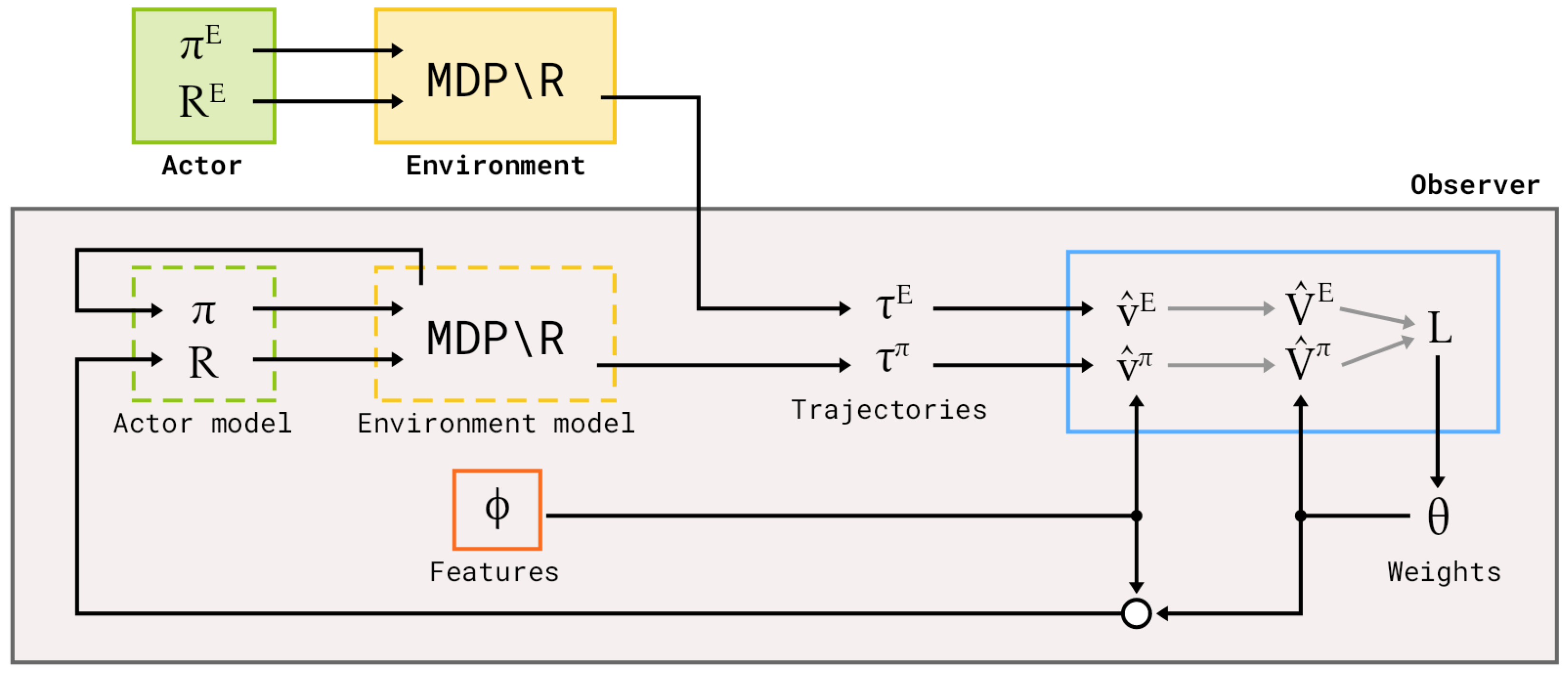
Given(1) measurements of an agent’s behaviour over time, in a variety of circumstances, (2) if needed, measurements of the sensory inputs to that agent, (3) if available, a model of the environment.
Determinethe reward function being optimised.
Under the principle of rationality, a rational agent’s behaviour is driven by a tendency to optimise for its desires given its beliefs. The intentional stance invokes this principle to attribute causality for behaviour to mental states [33]. An agent’s reward function is the driver of its behaviour and can therefore operate as a representation of its desires. On the other hand, the agent’s beliefs about the world inform what behaviour is appropriate or feasible, and play a crucial role in planning toward fulfilling its desires. IRL may serve as an algorithmic paradigm for inferring the mental states (beliefs, desires) of others based on their observed behaviour (i.e., ToM) [22].

2.1. Problem Formulation and Notation

The problem setting for IRL, as for RL, is a (finite) MDP, characterised by the tuple ( S , A , T , D , γ , R ) with
  • S = { s 1 , s 2 , } —a (finite) set of states
  • A = { a 1 , a 2 , , a k } —a finite set of k actions
  • T = { Pr ( s | s , a ) : s , s S , a A } —the state transition probabilities
    when performing a in s
  • D = { Pr ( s 0 = s ) : s S } —a probability distribution over S from
    which the initial state is drawn ( s 0 D)
  • γ [ 0 , 1 ) —a time discount factor
  • R : S × A R —a reward function whose absolute value
    is bounded by R m a x .
Behaviour within an MDP is dictated by a policy. A deterministic policy is a function π : S A , yielding an action choice a for a given state s. A stochastic policy is a probability distribution over actions given a state π ( a | s ) = P ( a | s ) . A mixed policy ψ is a distribution over a set of deterministic stationary policies Π , with λ k = P ( π = π k ) , or equivalently, a convex combination with coefficients k λ k = 1 . Mixed policies are executed by selecting a policy π k with probability λ k at the start of the MDP and following this policy for the entirety of the problem. A policy is optimal when it maximises its associated value function, or “expected sum of discounted rewards”,
V π = E ( s t , a t ) d π , T , t [ t = 0 γ t R ( s t , a t ) | D , T , π ] = E s 0 D [ V π ( s 0 ) ] ,
where d π , T , t is the state–action distribution at time t, a result of the agent’s policy and the environment’s transition probabilities, with s 0 drawn from D. The Bellman equation provides a way to recursively compute the values of states under a policy. For a given MDP, V π satisfies
V π ( s ) = R ( s ) + γ s S T ( s , π ( s ) , s ) V π ( s ) s S , a A .
An additional auxiliary function commonly used in MDP settings is the Q-function
Q π ( s , a ) = R ( s , a ) + γ s S T ( s , a , s ) V π ( s ) s S , a A ,
which defines the cumulative reward to be expected from performing action a while in state s, and can be used to obtain an optimal policy π ( s ) arg max a A Q π ( s , a ; R ) for a given R.
A useful representation of a policy is its discounted state–action visitation distribution, or occupancy. A policy π and its occupancy measure μ π can be used interchangeably for a given environment—occupancy provides a representation of the policy as influenced by the transition dynamics of the environment. By employing Kronecker delta notation ( δ i j = 1 if i = j , 0 otherwise), the occupancy is
μ π ( s , a ) = E ( s t , a t ) d π , T , t [ t = 0 γ t δ s t s δ a t a | D , T , π ]
and is sufficiently defined through the linear Bellman flow constraints [34]
μ π ( s ) = D ( s ) + γ s S a A μ π ( s , a ) T ( s , a , s ) , μ π ( s ) = a A μ π ( s , a ) , μ π ( s , a ) 0 .
These constraints define a set G of all the constraint-satisfying occupancies, each of which can be represented as a vector μ π R | S × A | [35].

2.2. IRL Concepts

The notation MDP∖R is used to denote an MDP where the reward function R is not given. The IRL task consists in finding an R for which the agent’s observed behaviour is optimal given an MDP∖R, usually working within a parametric class { R θ : θ Θ } . The canonical approach to this is to use a linear approximation of R from features ϕ ( s , a ) R d of each state and action, with weights θ R d , such that R ( s , a ) = θ T ϕ ( s , a ) . This is explained in further detail, with alternative approaches, in Section 3.2. The idea of approximating utility (reward) as a linear function of subutilities (features) dates back to the work of Carmel and Markovitch [36], used for opponent modelling in extensive form games (chess), and is closely related to earlier work in economics, such as in [37]. Often R, ϕ , are functions of the state only, instead of state–action pairs. The extension to this setting is trivial if we adopt the state–action formulation. Under a policy, we have feature expectations (expected discounted value of features) v π R d :
v π = E ( s t , a t ) d π , T , t [ t = 0 γ t ϕ ( s t , a t ) | D , T , π ] .
A feature matrix F R d × | S × A | can be employed to encapsulate the features for each state–action pair F ( · , s , a ) = ϕ ( s , a ) , resulting in v π = F μ π . Under a linear approximation of the rewards, V π (Equation (1)) can alternatively be obtained from features (through linearity of expectations) with
V π = θ T v π = θ T F μ π .
Feature counts from a given trajectory τ provide a compact representation of the trajectory
Φ j = Φ ( τ j ) = t = 0 H j γ t ϕ ( s t , a t ) R d .
The measurements of the behaviour of the agent of interest (here actor or expert) over time are given as demonstrations D , usually taking the form of an unordered set D = { τ j π } j = 1 m of sequential paths (i.e., trajectories) τ j π = ( ( s , a ) t ) t = 0 H j of length H j + 1 . Additional information may be provided in the demonstrations, including feature matrices, occupancies, etc.
Empirical estimates of occupancy and feature expectations can be computed as average counts from the observed trajectories
μ ˜ π ( s , a | τ j ) = 1 H j + 1 t = 0 H j γ t δ s t s δ a t a ,
v ˜ π = F μ ˜ π .
The above results all apply to mixed policies through linearity of expectations.

2.3. Boltzmann Policies

To make stochastic policies more robust to environmental changes, it is desirable that they assign nonzero probabilities to actions other than the optimal to allow for exploration. According to Jaynes’ Maximum Entropy Principle (MaxEnt) [38], to find a probability distribution that minimises bias for a given partial set of information requires maximising the amount of entropy (or uncertainty) in the distribution, subject to the known information. Recall the definition of a deterministic optimal policy through the Q-function (Equation 3)). To define a stochastic policy, a distribution over action choices can be determined from their associated Q-values instead. Subject to moment matching constraints for the zeroth and first moments
a A π ( a | s ) = 1 s S , E [ Q π ( s , a ) ] = a A π ( a | s ) Q π ( s , a ) s S ,
the entropy-maximising distribution is the Boltzmann distribution, or “Boltzmann policy” as it is known in the RL context,
π ( a | s ) = Pr ( a | s , R , π ) = 1 Z exp α Q π ( s , a ; R ) ,
with normalising constant, or partition function Z ( s , R , π , α ) = a A exp α Q π ( s , a ; R ) and (negative) potential energy Q π ( s , a ; R ) . The hyperparameter α serves as an inverse temperature parameter defining the steepness of the policy distribution, or how “greedy” for optimal Q-values it is. This greediness may be understood as the level of rationality attributed to the agent by the ToM observer. This distribution is known as the Softmax function in the machine learning literature.
A maximum entropy optimal policy can be obtained through the soft Q-function
Q soft π ( s , a ) = R ( s , a ) + γ s S T ( s , a , s ) V soft π ( s ) V soft π ( s ) log a A exp Q soft π ( s , a ) ,
where the value function is defined through the LogSumExp function [39]. Actions with higher Q-values reduce regret, which rational agents are expected to act in accordance with. An alternative and equivalent interpretation of this policy is as proportional to the exponential advantage of an action
π ( a | s ) exp Q π ( s , a ) V π ( s ) .
The Boltzmann distribution provides a smooth parametric model for the action choice distribution in a given state (i.e., a policy) that is shaped by the Q-function at the state. These qualities, along with the alignment with MaxEnt and the degree of freedom in the temperature hyperparameter, are desirable attributes in modelling rational agents. For these reasons, a sizable proportion of IRL algorithms resort to a Boltzmann assumption when characterising the policy (e.g., Section 3.1.1.6, Section 3.1.2.2, Section 3.1.2.3, Section 3.1.3.2 and Section 3.1.6.3). It is common practice to assume the Q-function is given in a converged state or obtained through dynamic programming (value iteration) or RL methods (e.g., Q-learning). In the ToM interpretation, the accuracy of the Q-function with respect to the true values of the MDP encode, in part, the accuracy of the agent’s beliefs—a core mental attitude of ToM, as discussed in Section 4. Another core mental attitude in models of ToM are desires, which are encoded as rewards in rational agent models. In the following section, we review IRL algorithms whose emphasis is on recovering these rewards, and discuss how they can provide an effective computational approach to inferring an agent’s desires from their behaviour.

3. Inferring an Agent’s Desires

The problem of inferring an agent’s desires with computer science methods was first approached by Russell [32], which coined IRL broadly, suggesting a possible algorithmic direction based on the use of a parametric form of the reward function, as is common in econometrics. In the IRL problem setting, this function can be fitted using Pr ( τ | R θ ) , the likelihood of observing behaviour τ if the true reward function were R θ , as a loss function. The parameterisation (or lack thereof) of R offers a design choice (see Section 2.2). Any optimisation method can be employed given this formulation, usually involving interleaving policy optimisation and reward function selection. However, there may exist multiple reward functions for which the observed trajectories are optimal, including degenerate solutions. This issue was the first to be addressed in the IRL literature [40], and provides our first classification axis for algorithms, namely by how they discriminate between plausible reward functions, as covered in Section 3.1. Another important concern is how the reward function can be characterised beyond a linear parameterisation, which we explore in Section 3.2.

3.1. Reward Function Discrimination

The first algorithmic treatment of the IRL task was by Ng and Russell [40], proving IRL soluble for moderately sized discrete and continuous state spaces. They characterised, analytically, the set of all reward functions for which a given policy is optimal for finite state spaces, and suggested heuristics to constrain said set of reward functions in the form of penalties for the cost of single-step deviations from the given (optimal) policy and regularisation of the rewards (modulated by hyperparameter λ ). For finite state spaces, R (and any other function of the states) can be represented as a vector R whose ith element is R ( s i ) . Similarly, the state transition probabilities can be encapsulated in a tensor T [ 0 , 1 ] | S | × | S | × | A | , which can be indexed by action to obtain a matrix T a where each ( i , j ) element is the probability of transitioning from state s i to state s j upon performing action a. In the resulting formulation, including the penalties, the goal is to find the R that maximises
s S min a A \ a 1 { ( T a 1 T a ) ( I γ T a 1 ) 1 R } λ | | R | | 1
with a 1 π ( s ) and subject to the constraints
( T a 1 T a ) ( I γ T a 1 ) 1 R 0 a A \ a 1 , | R ( s ) | R m a x s S ,
where ⪰ represents elementwise inequality (for all elements).

3.1.1. Maximum Margin Methods

3.1.1.1. Foundational Work

To extend the method to infinite state spaces, the authors resorted to a linear approximation of R with given fixed features. This approach to the problem is the canonical form of the so-called maximum-margin class of IRL techniques, the goal of which is to estimate a reward function that maximises the difference between an optimal policy and the rest of the available policies [27], or equivalently, a set of weights θ that parameterise a reward function R θ , such that under R θ , V π V π for all π . This particular method requires a way to approximate the value of V π under any MDP. Invoking Equation (7), the task is then to find the θ that maximises, for a sample S 0 S of the state space
s S 0 min a A \ a 1 { p ( E s T ( s , a 1 ) [ V π ( s ) ] E s T ( s , a ) [ V π ( s ) ] ) }
with
| θ i | 1 i = 1 , 2 , , d p ( x ) = x x 0 2 x x < 0 ,
where p is a penalty function for states in which π is not optimal under R ^ . The penalty weight value of 2 in p is arbitrarily chosen. The original paper asserts that results were not sensitive to this value.
Finally, further generalising the method, they introduced an algorithm to find R ^ such that a policy π to be determined maximises V π when a set D of trajectories τ through S is given in lieu of π E . This algorithm requires (i) a way to approximate V π (as above), (ii) a way to find an optimal policy π k under any R (techniques from the RL literature can be employed to this end), and (iii) the ability to simulate trajectories starting from s 0 under policy π in the MDP.
Approximations of the feature expectations and the value function can be obtained by performing m Monte Carlo trajectories of length H under π , and averaging over their values (for a large H, the difference as compared with an infinite time horizon is negligible):
v ˜ π ( s 0 ) = 1 m j = 1 m t = 0 H j γ t ϕ ( s t ( j ) )
V ˜ π ( s 0 ) = θ T v ˜ π ( s 0 ) .
Similarly, we can obtain approximations for the expert’s feature expectations, but note that their accuracy is contingent on the size of the set of demonstrations provided, as well as the fact that some states may not be visited in some cases.
In their final algorithm, shown in Algorithm 1, the optimisation step is similar to Equation (15), with the same constraints, but replacing the expectation by the empirical average V ˜ π from Equation (17), and the domain S × A \ a 1 by the set of policies Π . The initial state s 0 is fixed for all the trajectories, but this results in no loss of generality if we let s 0 be a dummy state and set T ( s 0 , a , s 1 ) = D ( s 1 ) for all a A .
Algorithm 1: Algorithm from [40]
Algorithms 16 00068 i001
In the context of ToM, the given trajectories represent the observer’s knowledge of the actor’s behaviour. The longer the trajectories and the larger the set of trajectories (hyperparameters H and m, respectively), the better the observer can be said to know the actor. The resultant R ^ is the observer’s model of what drives the actor’s behaviour (i.e., its utilities), which may be used in conjunction with policy estimates π Π (i.e., its probabilities) to predict its future behaviour. In Figure 1, we group these two variables together conceptually as the observer’s model of the agent (green, dashed outline). The rationality of the actor is based on these two sources of information [41]. The observer requires a model of the environment (MDP∖R) to be able to estimate the model of the agent. This is a sensible requirement for any agent. In Algorithm 1, it is assumed to be completely faithful to the real environment (Figure 1, yellow with dashed and solid outlines, respectively).
One outstanding question is the meaning of the basis functions, or environment features, ϕ i in the context of ToM. We place them conceptually within the observer, as depicted in Figure 1 (orange). The cardinality d of the space Θ in which we perform the linear approximation of the reward function, and thus its expressivity, depends on how many features the observer makes use of. Intuitively, they stand for the perceptual acuity of the observer—the number of different “stimuli” the observer can differentiate amongst and attribute value to. They are likely to differ to that of the actor; that is, if the actor does have them in the first place—it may not know its subutilities and simply be guided by its reward function. Simple examples of features in the scenario of an agent crossing the road include whether there is a car present, the speed of the car, the state of the pedestrian crossing traffic lights, etc. Moreover, not only the features, but the state observations themselves may differ between the actor and the observer (e.g., first-person vs. third-person point of view). In Ng and Russell [40] they are “given” and fixed.
As new trajectories are observed, the same algorithm can be used to update the weights if the current θ and π k are used instead of randomly initialising them. We call attention to the fact that, although this was not stated in the algorithm as presented, it can yield the set of policies π Π , as well as their respective v ˜ π , V ˜ π , and different reward function estimates R ^ under which each of the policies were optimised.

3.1.1.2. Feature Expectation Matching

Abbeel and Ng [42] contributed modifications to the max-margin approach under somewhat stricter constraints: R is bounded in absolute value to 1, which requires | | θ | | 1 1 , and therefore | | θ | | 2 1 . Casting the problem as apprenticeship learning (AL), deviating slightly from the IRL premise, their goal is to find a policy π that performs close to the expert policy under the unknown reward function R . Their focus is on the feature expectations: the estimated policy π must obtain (empirical) feature expectations close to the expert’s, i.e., satisfy | | v π v π E | | 2 ϵ . In other words, the true goal is not uncovering the reward function: although the algorithm guarantees finding a policy, the feature expectations of which are within ϵ of the expert’s, the reward function recovered as part of this process may not be correct. Because the 2 -norm of the linear approximation weights θ is restricted to be less than 1, this is equivalent to minimising the difference between the value functions of the expert’s ( π E ) and estimated ( π ) policies. Such policy (and pertaining feature expectations) can be obtained almost identically to Algorithm 1, with the key difference being in the weights’ update step, as per Algorithm 2, and the change in the loop exit condition to t < ϵ . They provide an additional, simpler algorithm based on computing the orthogonal projection of the feature expectations onto the segment between previous iterations’ expectations and demonstrate its faster convergence compared to their max-margin method.
Algorithm 2: Excerpt from the algorithm in [42], with adapted notation.
Algorithms 16 00068 i002

3.1.1.3. Multiplicative Weights Apprenticeship Learning

Syed and Schapire [43] expand on the apprenticeship learning algorithm in [42] with algorithmic tools from game theory. Further constraining the ranges of ϕ ( s ) [ 1 , 1 ] d and θ Θ C = { θ R d : | | θ | | 1 = 1 and θ 0 } allows for defining the margin V π V π E min i { v i π v i π E } to be maximised. The goal is defined through the game value (note the difference in symbols ν , v)
ν = max ψ Ψ min θ Θ C θ T v ψ θ T v E ,
i.e., ψ is the mixed policy that maximises V ψ V π E for the worst-case possibility for θ , a sensible constraint because θ is unknown. This allows for a zero-sum game formulation, though only abstractly, so the “players” are not the observer and actor, but the rewards and the policy (this is the foundational concept of adversarial IRL methods, reviewed in Section 3.1.7). “Min player” sets the reward by choosing θ , and “max player” chooses a mixed policy ψ , adversarially. As such, the game can be defined via a d × | Π | game matrix with G ( i , k ) = v k ( i ) v E ( i ) , where i indices over the feature dimensions d and k over the policies in Π , the space of policies π . From this, we have
ν = max ψ Ψ min θ Θ C θ T G ψ = min θ Θ C max ψ Ψ θ T G ψ 0
in Von Neumann’s minimax form [44]. The 0 lower bound is explained as follows. The stricter constraint setting θ Θ C is equivalent to assuming all the features “got the sign right” in relation to how they contribute to the reward (because the weights are all positive). This assumption results in ψ having higher value than π E when v ψ v π E regardless of the value of the actual weights θ .
To solve this optimisation problem, they adapt the multiplicative weights algorithm from [45]. This algorithm has two main steps. (1) Given min player “strategy” θ , find ψ = arg max ψ Ψ θ T G ψ (i.e., find an optimal policy in the MDP with known R, through any MDP solver); (2) Given max player “strategy” ψ , compute ( θ ˙ ( i ) ) T G ψ for each of the d pure (i.e., one-hot) strategies θ ˙ ( i ) (i.e., compute the feature expectations v R d of the given policy ψ , which can be done by solving d systems of linear equations, or approximated iteratively). These steps in Algorithm 3 are equivalent to the projection algorithm from [42]. The complexity of these steps scales with the size of MDP∖R, and not with G. There is similarity in the higher bound approximation step in [46] (Algorithm 4, line 12).
The mixed policy returned by the Multiplicative Weights AL algorithm consists of a uniform distribution over estimated policies π ^ that are ϵ π -optimal, meaning | V ( π ^ ) V ( π ) | ϵ π . The game matrix G is slightly modified and makes use of ϵ v -good feature expectations estimates, meaning | | v ^ v π | | ϵ v .

3.1.1.4. Linear Programming Apprenticeship Learning

The nondeterministic nature of mixed policies may not be desirable. Later work by Syed et al. [34] demonstrated that stationary policies can be obtained from Algorithm 3 by finding the optimal policies through linear programming, showing up to two orders of magnitude improvement in running time. The resultant linear program to find the maximum margin is
max ν R , μ π G ν
subject to
v i F i ( μ π μ E ) i = 1 , , d
with resulting stationary policy
π ( a | s ) = μ π ( s , a ) a A μ π ( s , a ) .
Empirical estimates for occupancy values can be obtained from given trajectories by using Equation (9).
Algorithm 3: Multiplicative Weights Apprenticeship Learning (MWAL) Algorithm [43]
Algorithms 16 00068 i003
The last three methods we reviewed [34,42,43] are instances of AL. Although the objective in AL is to learn a policy that resembles the expert’s, as opposed to learning the reward function, AL and IRL are largely overlapping and share core techniques, specifically in the two main tasks of policy estimation from observed behaviour (goal of AL), and the inference of rewards from a given policy (goal of IRL). Knowing an agent’s policy may also be considered a form of ToM, as it is internal to the agent and reflects their intentions/modus operandi. The use of these two core tasks in ToM may be better understood through a simile with the “theory theory” and the simulation theory accounts of mentalising. The theory theory perspective assumes that we make inferences about hidden mental states through logic and abstraction, as we do in the natural sciences for the unobservable causal phenomena of the world. This is similar to the reward learning approach. In the “simulation theory” account, mental states are represented through perspective-taking, by using our own cognitive resources to simulate another’s [47,48]. This is similar to the AL approach (e.g., [42,49]), as well as the less-sophisticated behavioural cloning (BC), whereby agents learn state–action mappings through supervised learning (with the limitation in applicability to observed state–action pairs only). The simulation account can be extended to IRL. For example, in [50] the observer models a human’s reward function by proposing counterfactual scenarios.

3.1.1.5. Maximum Margin Planning

The use of (estimated) state–action occupancy measure from demonstrations is further extended by Ratliff et al. [49], whose goal is to find a reward function under which the optimal policy is similar to the expert’s. To do so, they cast the problem as structured prediction, relying on a loss-augmented reward function R l = θ T F j + l j T , where l j R + | S × A | is a loss vector defining the cost of deviating from the expert policy for every state–action pair.
Each demonstration may be generated in a different MDP, and is given by D = { ( S , A , F , G , μ , l ) j } j = 1 m . From this, they introduce an objective function measuring the difference in performance between a policy with occupancy μ θ = arg max μ G j ( θ T F j + l j T ) μ (optimal under the loss-augmented reward function), and the given demonstration μ j (without loss-augmentation), based on a quadratic programming formulation (in accordance with the hinge loss form)
c q ( θ ) = 1 m j = 1 m β j θ T F j + l j T μ θ θ T F j μ j q + λ 2 | | θ | | 2 .
The form of the loss function imposes a margin by which the solution obtained is better than any other possible solutions. Using the occupancy measures from the expert policy has the effect of making rewards for high occupancy state–action pairs larger, which in turn encourages similarity between the policies, as well as discouraging degenerate solutions [51]. The optimisation of the weights θ is performed through gradient descent by using the subgradient of the objective function
g θ q = 1 m j = 1 m q β j θ T F j + l j T μ θ θ T F j μ j q 1 F j ( μ θ μ j ) + λ θ ,
where β j is a data-dependent normalisation coefficient, q { 1 , 2 } is a choice of slack penalty type (for 1 - and 2 -loss, respectively). Boularias and Chaib-draa suggest the use of a loss vector l ( s , a ) = 1 μ j ( s , a ) [35]. The (near-)optimal policy π θ is obtained with RL methods in the particular MDP∖R under the loss-augmented reward function, and provides the occupancy μ θ . Optionally, the weights θ can be projected on to additional problem-specific constraints after every update. The weights can be learned offline from a training set D , or online for each observation D j . The occupancies μ j can be obtained equivalently from trajectories τ j when the demonstrations are in said format instead.
Prior knowledge can be included in the form of further constraints on θ , such as by explicitly penalising certain features, or regularising the learning procedure around a prior belief about θ instead of approximately 0. Additionally, it can be included through the loss vector l if certain state–action pairs are known to be poor choices [49].
When there is no single reward function that maximises the margin, such as when the agent’s behaviour is suboptimal or no data is available for parts of the state space, this method is limited [52].

3.1.1.6. Policy Matching

Neu and Szepesvári [53] set out to find a θ for which π θ matches the expert policy π E , or rather the empirical occupancy estimate μ ˜ π E thereof, through gradient descent on a loss function (similar to [49]). Thus, their performance measure is the difference between the proposed and expert policies, as opposed to the proposed policy’s performance with respect to the original reward function as is the case in [42]. They select the squared loss function
L ( μ θ ; μ E ) = s S , a A μ θ ( s , a ) μ E ( s , a ) 2
and assert it can be approximated by
L ( μ θ ; μ E | τ E ) = s S , a A μ θ ( s , a ) μ ˜ E ( s , a | τ E ) 2 .
Obtaining the occupancies μ θ requires a policy π θ . They employ a Boltzmann policy (Section 2.3), acting as a smooth map from the parameter space to the policy space. As in [49], the parameterised policy π θ is trained through an MDP solver to be (near-)optimal under R in the MDP∖R. The reward function parameters are obtained through gradient descent on the loss function. Others have taken a similar approach of matching the expert’s state occupancy through gradient techniques [54].

3.1.2. Probabilistic Methods

Probabilistic methods cast the IRL problem as a (Bayesian) inference problem, aiming to find an estimate for R that best explains the given demonstrations (interpreted as noisy observations of the expert’s policy) [55]. The agent’s action choice probabilities Pr ( a | s , R E ) are modelled as a Boltzmann distribution (Section 2.3) (or alternatively made deterministic as arg max a A Q ( s , a ; R E ) ). This allows us to define the likelihood of a pair ( s , a ) S × A under any given R as
Pr ( ( s , a ) | R ) = exp α Q ( s , a ; R ) a A exp α Q ( s , a ; R ) .
Under an assumption of independence between state–action pairs in a given demonstration (based on a stationarity assumption for the agent’s policy), the likelihood of the demonstration is
Pr ( D | R ) = ( s t , a t ) D Pr ( ( s t , a t ) | R ) .
Combining the likelihood from the demonstrations with a given prior over rewards P ( R ) , we can obtain a posteriori
Pr ( R | D ) = Pr ( D | R ) Pr ( R ) .
Two solution methods are used to find this posterior in the literature: gradient-based methods are used to directly find an (approximate) maximum a posteriori estimate for R, and Markov chain Monte Carlo (MCMC) methods to approximate the entire posterior distribution of R [55]; more recently, variational inference-based methods have been proposed to this end, e.g., [56,57,58].

3.1.2.1. Tree Traversal

Chajewska et al. [46] provide the first algorithm to treat the reward as a random variable. Of further interest to this review, they show the usefulness of their method for strategic interactions in the two-player game setting. They work with a game decision tree instead of an MDP (though the method can equivalently be applied in the MDP setting), allowing the observer to consider the actor’s actions as well as their own and “nature”/chance decision nodes.
Similarly to [40], they use τ E to fit linear constraints on Θ , a space of coefficient values for a linear approximation of R. They set out to obtain a posterior distribution q ( θ | τ ) over a constrained region of the parameter space Θ C , by conditioning a prior p ( θ ) on the evidence from the demonstrations Pr ( τ | θ ) . The constrained region Θ C is contained in Θ [ 0 , 1 ] d , the polytope defined by V π V π π Π . The prior p ( θ ) over Θ is obtained through density estimation on population reward function data (from many actors, as in e.g., [41]). Because q ( θ | τ ) can be prohibitively complex to compute, the method approximates it through an MCMC procedure (Algorithm 4), specifically by using the Metropolis–Hastings (MH) algorithm over a quantisation of the convex set Θ C , with p as the acceptance probability distribution.
Θ C is obtained by traversing the tree and assigning upper ( V hi ( s ) ) and lower ( V lo ( s ) ) bounds on the value of each node, V lo ( s ) V ( s ) V hi ( s ) , with the set of constraints C built with constraints V hi ( s ) V lo ( s ) from each of the expert’s decision nodes. We use S ( s ) as shorthand for the subset of S that is reachable from s, i.e., S ( s ) = { s : T ( s , a , s ) > 0 a A } . The use of π E ( s ) denotes choices that are perceived as chance by the expert, including the observer’s actions and nature’s actions (passive dynamics). Although the original paper did not, we make use of the Bellman equations in our elucidation of the algorithm where applicable, for closer correspondence with IRL. The algorithms are equivalent if γ = 1 and ϕ ( s ) = 0 for all s that are not leaf nodes.
Algorithm 4: Metropolis–Hastings-based approach to approximate q ( θ | τ ) from [46]
Algorithms 16 00068 i004

3.1.2.2. Policy Walk

Ramachandran and Amir [59] formally state the problem as Bayesian inference (hereafter Bayesian IRL). Their PolicyWalk MH algorithm (Algorithm 5) allows for domain knowledge to be incorporated in the prior, with the potential for further improvement in estimation accuracy.
Their approach models the likelihood of state–action pairs as the occupancy under the expert’s policy Pr ( ( s t , a t ) | R ) = μ E ( s t , a t ) with a Boltzmann distribution assumption (Section 2.3). Unlike its use in [53] (Section 3.1.1.6), here the normalisation in the likelihood has to be done over all ( s t , a t ) τ , which may be intractable depending on the state space. Fortunately, because the algorithm only uses ratios of the densities, the normalising constant Z can be discarded, and the resultant likelihood is
Pr ( τ | R , π ) exp α ( s t , a t ) τ Q π ( s t , a t ; R ) ;
hence, the posterior is
Pr ( R , π | τ ) p = exp α ( s t , a t ) τ Q π ( s t , a t ; R ) Pr ( R ) ,
where p is used as the acceptance probability distribution in the MH procedure.
Algorithm 5: Policy Walk Algorithm [59]
Algorithms 16 00068 i005
For the prior Pr ( R ) , they invoke the principle of maximum entropy to assume the rewards are independent and identically distributed. Three different prior distribution candidates are proposed:
  • for prior-agnostic context, a uniform distribution over [ R max , R max ] | S | or an improper prior Pr ( R ) = 1 over R | S | ;
  • for real-world MDP with parsimonious reward structures, a Gaussian or Laplacian prior (over R | S | ); and
  • for planning-type problems, where most states can be expected to have low or negative rewards, with some having high rewards, a Beta distribution (over R | S | ).
An important distinction is that the PolicyWalk algorithm estimates the value of R at each of the states directly, and therefore it does not make use of features or a (linear) function approximator for R as in the previously discussed methods. Although they show substantial improvements over the method in [40] for | S | 1000 , larger (or infinite) state spaces may not be feasible to learn over with this approach. The loss functions used in their evaluation experiments are the 2 -norm between the estimated and true reward functions R, and the 1 -norm for the estimated policy π evaluated under the true R. Bayesian IRL methods are limited in scalability, as they have to define probabilities and/or calculate value or quality function values for every point in the state–action space. Furthermore, as in other previous methods, large computational overheads are associated with the need to optimise the policy in the MDP.
The authors posit that the max-margin method from [40] is a special case of Bayesian IRL where the obtained R is the MAP estimate with a Laplacian prior. This argument is later extended by Choi and Kim [60] (Section 3.1.4). The solution space for this method is the same as in [53], as per the analysis in [61].

3.1.2.3. Structured Generalisation

Rothkopf and Dimitrakakis [62] contribute a principled generalisation of the Bayesian IRL approach (Section 3.1.2.2) with structured priors on rewards and policies. Given a controlled Markov process ν = { S , A , T } and a discount factor γ (or priors thereof), a prior for a stochastic reward function Pr ( ρ | ν ) over the space of reward functions R , and a prior for the policy Pr ( π | ρ E , ν ) over the policy space Π ; with joint prior π P Π , ρ R R
Pr ( π , ρ | ν ) ρ R Pr ( π | ρ , ν ) d Pr ( ρ | ν )
the posterior on reward functions is
Pr ( ρ | τ , ν ) = Pr ( ρ | s 1 : H , a 1 : H , ν ) = ρ Π π ( a 1 : H | s 1 : H ) d Pr ( π | ρ , ν ) d Pr ( ρ | ν ) R Π π ( a 1 : H | s 1 : H ) d Pr ( π | ρ , ν ) d Pr ( ρ | ν ) .
With this statistical model and the usual Boltzmann action choice probability assumption (Section 2.3), they derive two MH algorithms: direct sampling from the joint posterior distribution Pr ( π , ρ | τ ) , and a hybrid Gibbs sampler procedure with a reward sequence augmentation of the model with Pr ( r t | s t , a t , ρ E ) . These algorithms do not require the demonstrations to be optimal, and are capable of finding policies that outperform the agent’s actual policy with respect to its reward function, as well as revealing policies that perform better than those recovered with previous IRL methods.

3.1.3. Maximum Entropy Methods

Bayesian IRL methods compute the likelihood as the total probability over each action choice in a trajectory. This fails to account for global interdependencies of choices along a trajectory. Maximum entropy methods focus on modelling the likelihood of entire trajectories Pr ( τ | R ) as a whole, as opposed to individual action choices. They resolve the ambiguity between trajectories, constrained to matching feature counts by maximising the entropy of the distribution.

3.1.3.1. Maximum Entropy IRL

Ziebart et al. [52] provided a definitive method by which to discriminate between reward function candidates by focusing on the characterisation of the likelihood Pr ( τ | θ ) . Although previous probabilistic approaches worked with distributions over policies, inevitably focusing on local action choices [53,59], this method is based on a distribution over entire trajectories that is normalised globally. Multiple trajectories with the same feature counts may obtain the same rewards under a given R θ . Through the principle of maximum entropy, they obtain a distribution that removes any preferences for trajectories beyond the requirement of matching feature counts, thereby resolving the ambiguity. It attributes equal probabilities to trajectories with equal rewards, and exponentially higher probabilities to trajectories with higher rewards, and does so globally over the trajectories (as opposed to locally at the action level as is the case in [49,59]).
For observed trajectory realisations τ j = 1 : m E , this is equivalent to maximising the likelihood of the observed trajectories under a maximum entropy exponential family of distributions ( exp θ T Φ ( τ ) ) θ Θ . Thus, learning from observation entails finding θ = arg max θ L ( θ ) , where
L ( θ ) = τ j = 1 : m E log Pr ( τ j E | θ , T ) .
With a partition function Z assumed constant for all ( s , a , s ) , and assuming the effects of transition dynamics on behaviour are negligible, the distribution of interest for nondeterministic MDPs (which extends trivially to deterministic MDPs) is
Pr ( τ | θ , T ) = ( s , a , s ) τ T ( s , a , s ) exp θ T Φ ( τ ) Z ( θ , s , a , s ) exp θ T Φ ( τ ) Z ( θ , T ) ( s , a , s ) τ T ( s , a , s ) .
The gradient of L ( θ ) is the difference between the average feature counts from observed trajectories and the expected feature counts over all trajectories in the MDP. The latter can be expressed equivalently taking the expectation over states in the MDP instead, requiring the state visitation frequencies μ θ ( s )
L ( θ ) = 1 m j = 1 m s t τ j E ϕ ( s t ) τ [ Pr ( τ | θ , T ) s τ ϕ ( s ) ] = Φ ˜ ( τ j = 1 : m E ) E τ [ Φ ( τ ) | θ , T ] = Φ ˜ ( τ j = 1 : m E ) E s [ ϕ ( s ) | θ , T ] = 1 m j = 1 m Φ ( τ j E ) s S μ θ ( s ) ϕ ( s ) .
Thus, for the optimal θ , the feature expectations over the MDP match the empirical feature expectations from the observed trajectories. The state visitation frequencies μ θ ( s ) for an infinite time horizon can be approximated for a large time horizon H by using a sample-based algorithm (Algorithm 6). The above is equivalent to calculating the feature expectations v ˜ π with γ = 1 ; thus, here too we try to minimise the difference between trajectory values between observed trajectories and trajectories from parameterised policy, but avoid actually computing the policy in favor of using state occupancies obtained with Algorithm 6.
This approach is resilient to expert behaviour being suboptimal (cf. Section 5.1), as well as the stochasticity of the environment. Although the algorithm is efficient by using all paths below a fixed length, in their experiments with taxi driver path data Ziebart et al. [52] work within a smaller, fixed class of reasonable trajectories resulting in significant improvements in speed.
Algorithm 6: Maximum Entropy IRL Algorithm [52]
Algorithms 16 00068 i006

3.1.3.2. Maximum Causal Entropy IRL

Transition dynamics play an important role in MDPs. Ziebart et al. [39] frame the agent’s decision making in the MDP as two interacting stochastic processes: the environment’s transition dynamics T (assumed to be known—given or estimated from data), and the agent’s policy π (unknown in the IRL problem). For each time step t in the sequence ( 1 , , H ) , the state and action values are random variables S t , A t . These can be collected into the random sequences S 1 : H , A 1 : H , respectively, and they determine the interaction between the processes. When considered together, they form a trajectory τ .
In the MaxEnt approach [52], information is lost by failing to consider causality (time direction) in the trajectory distribution Pr ( τ | θ , T ) Pr ( S 1 : H , A 1 : H ) . This is addressed in [39,63] by proposing to use an alternative way to decompose this joint probability by using causally conditioned probabilities [64],
Pr ( S 1 : H , A 1 : H ) = Pr ( S 1 : H | | A 1 : H 1 ) Pr ( A 1 : H | | S 1 : H ) = t = 1 H Pr ( S t | S 1 : t 1 , A 1 : t 1 ) t = 1 H Pr ( A t | A 1 : t 1 , S 1 : t )
wherein future state variable outcomes have no effect on preceding variables. The state transition dynamics follow the Markov property, and thus have a causally conditioned probability T ( S 1 : H | | A 1 : H 1 ) = t = 1 H T ( S t , | S t 1 , A t 1 ) . An agent’s policy can also be modelled as a causally conditioned probability distribution, though the factors in the product of probabilities may not be Markovian, so π ( A 1 : H | | S 1 : H ) = t = 1 H π ( A t , | A 1 : t 1 , S 1 : t ) . The goal in this framing of the IRL problem is to find the maximum causal entropy (MaxCausalEnt) policy estimator
π ^ = arg max π ^ ( A 1 : H | | S 1 : H ) E τ [ log π ^ ( a 1 : H | | s 1 : H ) ] ,
such that
E τ Φ ( τ ) = Φ ˜ ( τ E ) ,
A t Pr ( A t | S 1 : t , A 1 : t 1 ) = 1 S 1 : t , A 1 : t 1 .
Assuming, as is usually the case, that the features decompose linearly in time makes the optimisation much simpler. The distribution (first-order Markovian policy) that optimises this constrained problem is a Boltzmann policy (Section 2.3) and takes the recursive form
π θ A t S t = Z A t S t , θ Z S t , θ log Z A t S t , θ = θ T ϕ S t , A t + S t + 1 P S t + 1 S t , A t log Z S t + 1 , θ log Z S t , θ = log A t Z A t S t , θ = LogSumExp A t { log Z A t S t , θ } .
An estimate of θ can be obtained through optimisation on the gradient computed through the calculation procedure in Algorithm 7. MaxCausalEnt was later expanded to the infinite time horizon setting [65,66].
Algorithm 7: Maximum causal entropy algorithm [63,67]
Algorithms 16 00068 i007

3.1.3.3. Extensions

Though the MaxEnt approach was groundbreaking and has been adopted as the de facto canonical model for IRL, it shares shortcomings with other previous methods, such as reliance on the feature map ϕ being given, and on a defined model T of the environment’s transition dynamics. Work that addresses these issues is exposed in Section 3.2 and Section 4.1, respectively. Boularias et al. [68] provide a model-free method based on minimising the relative entropy (KL-divergence) between the empirical distribution of trajectories produced by a baseline policy and the distribution of demonstrated trajectories produced by a learned policy. With p ( τ ) = Pr ( τ ) defined over the space of possible trajectories, and p π , T ( τ ) = Pr ( τ | π , T ) the probability of a trajectory under a policy and transition dynamics, the objective is
min p τ p ( τ ) ln p ( τ ) p π , T ( τ )
with constraints
| E τ [ Φ ( τ ) ] Φ ˜ i ( τ E ) | ϵ i i = 1 , , d p ( τ ) 0 τ τ p ( τ ) = 1 .
The objective is minimised through stochastic gradient descent, and this method is capable of learning from small demonstration samples. More recently, Snoswell et al. [69] provide a model-free MaxEnt IRL method based on a unified view of the MaxEnt and relative entropy methods that is capable of handling trajectories of variable lengths (with time complexity linear in longest trajectory length), state-dependent action spaces, and nonlinear reward characterisations (Section 3.2). An approach that is similiar to MaxEnt IRL and extends to continuous time and continuous state and action spaces is presented in [70]. Others have explored the use of semisupervised techniques by including unsupervised trajectories in addition to expert trajectories in training [71]. Connections of MaxEnt IRL with GAN and energy-based models have been drawn [72].
The MaxCausalEnt IRL method has been improved by including both (labelled) successful and failed demonstrations [73], and by considering its performance degradation as a result of diverging transition dynamics models in the agent and observer [74]. Its connections to other methods from econometrics have been studied under a unified perspective [75].

3.1.4. MAP Inference Generalisation

We have seen ways to obtain the posterior reward distribution for given trajectories through Bayesian and maximum entropy methods. Choi and Kim [60] analyse how best to obtain point estimates for the reward function from the posterior. Although the posterior mean is commonly used because it minimises the mean squared error, this measure entails integrating over the entire space of reward functions, including those that are not consistent with observed behaviour. Motivated by this issue, the authors suggest the MAP estimate as a more robust alternative and introduce a gradient method by which to obtain MAP estimates of the reward function, based on the (sub)differentiability of the distribution. In an effort to unify previous methods under the Bayesian perspective, they demonstrate that most of the IRL methods can be alternatively viewed as finding the MAP estimate, because they work by maximising an objective (equivalent to the posterior in Bayesian terms) that is comprised of an assessment term measuring compatibility between the reward and the demonstrations (equivalent to the likelihood in Bayesian terms), and a regularisation term measuring preference over realisations of the reward function (equivalent to the prior in Bayesian terms).
The ability to use prior knowledge to model an agent’s reward function is an important point from the ToM perspective. Actions alone do not provide enough information about the desires driving them, and there is great advantage in utilising information from other sources, such as task context or the type of actor [22], which can be incorporated in the form of priors in probabilistic approaches. For example, in the algorithm in [59] (Section 3.1.2.2) the observer has two “preconceptions” of the actor: the temperature α , representing how capable of choosing high-valued actions the observer expects the actor to be, and the prior Pr ( R ) , a distribution over the reward functions that may be chosen based on the type of actor or environment. Moreover, working with uncertainties may be useful to the observer. In an interactive setting, they may choose to act more conservatively when there are high uncertainties, or act to elicit more information from the actor to improve the confidence in the reward function estimate.

3.1.5. Linearly-Solvable MDPs

A severe limitation of the approaches we have reviewed thus far is their requirement to solve the forward MDP on each iteration, which comes at a high computational cost. Dvijotham and Todorov [76] present a method based on linearly solvable MDPs (LMDP) [77], which was the first to not require solving the forward problem. LMDP provide an approximation to MDPs that enables finding solutions faster at a small cost in accuracy. This is achieved through a decomposition of the dynamics into the environment’s passive dynamics Pr ( s | s ) (not to be confused with transition dynamics Pr ( s | s , a ) ), assumed to be given, and the control dynamics π ( s | s ) (not to be confused with the policy π ( a | s ) , though they are closely related).
The reward function (here, cost to be minimised) R comprises a state term r ( s ) 0 (to be inferred) and a control term that is the KL-divergence between the control dynamics and the passive dynamics (in order for the KL divergence to be defined, it is required that π ( s | s ) = 0 when Pr ( s | s ) = 0 , a condition that is imposed),
R ( s , π ( · | s ) ) = r ( s ) + D K L ( π ( · | s ) | | Pr ( · | s ) ) .
A desirability function z ( s ) = exp V ( s ) is used to define the optimal control dynamics
π ( s | s ) = Pr ( s | s ) z ( s ) ζ Pr ( ζ | s ) z ( ζ ) .
When the demonstration sample size is larger than the number of states, the method can recover the value function analytically, as the MLE of the unconstrained, convex function
Pr ( τ | V ) = s μ ˜ E ( s ) V ( s ) + s μ ˜ E ( s ) log s Pr ( s | s ) exp V ( s ) ,
which is uniquely defined. The policy and reward function are subsequently recovered from the value function estimate through z ( s ) . When the size of the demonstration sample is smaller than the number of states, the (negative) likelihood can be optimised with respect to z ( s ) instead, although the resulting function is nonconvex and its optimisation is slower and susceptible to local minima.
The value function can be represented as a look-up table or approximated as a linear function of features. Additionally, they suggest a method to automatically initialise and adapt the features in continuous space, employing Gaussian radial basis function kernels. A further potential advantage of this method is that it does not require trajectories ( s , a ) , operating over state transitions ( s , s ) instead.
Under passive dynamics, Pr ( τ | s 0 ) = t = 1 H Pr ( s t | s t 1 ) is the probability of a trajectory. For the same trajectory to occur when the control dynamics are applied, the probability is
Pr ( τ | s 0 , π ) = Pr ( τ | s 0 ) exp t = 0 H r ( s t ) z ( s 0 ) .
Note the similarity with MaxEnt IRL. Under uniform passive dynamics, MaxEnt IRL is an equivalent approach for LMDP.

3.1.6. Direct Methods

Direct methods take a more analytical approach to solving the IRL problem, exploiting the algebraic structure of the problem definition. Two classification methods proposed by Klein et al. [78,79] address the important limitation in previous work of needing to solve the MDP at every iteration. Orthogonally, two policy search methods operate through direct loss minimisation [80] and policy gradient minimisation [81].

3.1.6.1. Structured Classification-Based IRL

In Klein et al. [78], a multinomial classification with output labels for each action a A is trained to yield a classification score given the states. The critical insight is that the classification score q ( s , a ) can be interpreted as a proxy for the Q ( s , a ) function, assigning a value to each state–action pair. This additionally affords a policy approximator π C ( s ) = arg max a q ( s , a ) (Equation (3)). The training dataset comes from expert trajectories D C = { ( s t , a t = π E ( s t ) ) t } .

3.1.6.2. Cascaded Supervised IRL

Subsequent work by Klein et al. [79] retrieve a reward function estimate by chaining two generic supervised learning steps. First, a multinomial classification step yields a Q-function surrogate q, as in [78]. If the transition dynamics for the environment are known, a reward function can be obtained directly based on the Bellman equation from this classifier:
R ( s , a ) = q ( s , a ) γ s T ( s , a , s ) q ( s , π C ( s ) ) .
A key contribution of this work is removing the requirement of knowing the transition dynamics by approximating R through regression, as the second step in the process. Although the regressors ( s , a ) are provided, this requires a response variable r ^ , obtained from the Bellman equation with
{ r ^ t = q ( s t , a t ) γ q ( s t + 1 , π C ( s t + 1 ) ) } t .
The resultant dataset is D R = { ( s t , a t ) , r ^ t } t . However, samples for state–actions that differ from the expert’s ( s k , a a k ) are needed to reduce the regression error. The authors address this with a synthetic augmentation of the regression dataset with artificial samples ( ( s t = s k , a ) , r l o ) t , a π E ( s t ) . The reward for these samples is set to ensure it is always lower than that of the expert’s samples: r l o = min k r ^ k 1 .

3.1.6.3. Empirical Q-Space Estimation

Melo et al. [61] provide analytical solutions to the IRL problem through constraints imposed by the policy observations, which can be optimal, perturbed, or incomplete. The so-called inverse Bellman equation
R ( s , a ) = Q ( s , a ) γ s S T ( s , a , s ) a A π ( s , a ) Q ( s , a )
shows a one-to-one relationship between Q-functions and rewards. If the transition dynamics are known, all we need to obtain a valid R is the Q-function, because the optimal policy is assumed to be either deterministic (Equation (3)) or Boltzmann (Equation (11)). Given the demonstrations and a prior on policies we can obtain an empirical Bayesian estimate of the policy π ^ ( s , a ) . If the optimal policy is known for a given state, we have Q ( s , · ) = 0 for actions that are suboptimal and uniform across the optimal actions. If the optimal policy is noisy, Q ( s , a ) = log ( π ^ ( s , a ) ) α + V ( s ) and we can set V arbitrarily. If no information is available for the policy at a given state, invoking the advantage function A ( s , a ) = Q ( s , a ) V ( s ) we have multiple degrees of freedom: arbitrary V ( s ) , and A ( s , · ) constrained to be 0 and have at least one zero-valued element because every state has at least one optimal action.

3.1.6.4. Direct Loss Minimisation

Doerr et al. [80] propose performing direct (deterministic) policy search on a reward function R j ( τ ) = L ( τ j , τ ) that reflects the loss between observed ( τ j ) and proposed ( τ ) trajectories. That is, optimise the reward parameterisation weights through
c ( θ ) = j M R j ( τ )
where τ is a trajectory under parameters θ (e.g., generated by the optimal policy for R θ ) in the same MDP as the demonstrations. Any off-the-shelf policy search method can be used to optimise θ , with the authors employing the covariance matrix adaptation evolutionary strategy (CMA-ES) optimiser.

3.1.6.5. Policy Gradient Minimisation

An alternative direct method is to find the reward function for which the parameterised policy gradient is minimised, as is done by Pirotta and Restelli [81] and Metelli et al. [82]. This removes the need for solving the MDP.

3.1.7. Adversarial Methods

Ho and Ermon [83] introduced a model-free adversarial framework to learn a policy, which is trained through RL under a reward function obtained through MaxCausalEnt IRL. Although this work did not contribute new IRL algorithms, it proposed a new framing of the problem analogous to generative adversarial networks (GAN) [84].
In tasks with large state–action spaces or unknown transition dynamics, the computation of the partition function in the MaxEnt objective is intractable [85]. Adversarial IRL methods [72,86] approximate the MaxEnt objective through sampling. A synthetic policy π ω generates trajectories maximising an entropy-regularised policy objective E [ t R ^ θ ( s t , a t ) log π ω ( a t | s t ) ] , whereas a binary discriminator
D θ ( s , a ) = exp R ^ θ ( s , a ) exp R ^ θ ( s , a ) + π ω ( a | s )
discerns between synthetic and expert trajectories. The two networks are trained adversarially, resulting in a reward function approximator R ^ θ and a policy π ω . This shares similarities with the earlier approach in [43] (Section 3.1.1.3).
The adversarial IRL approach has been extended for metalearning [85,87] (Section 6); improved with an information bottleneck [88], semantic rewards [89], or end-to-end differentiability through self-attention [90]; and adapted to language-conditioned tasks [91].
In this subsection, we have outlined the many approaches that have been proposed to discriminate between the several reward functions that could explain a given set of behavioural demonstrations. Maximum margin methods do so by attempting to maximise the margin between the chosen reward function and any other alternatives (Section 3.1.1). Probabilistic methods interpret the rewards as a random variable and the state–action pair demonstrations as evidence, framing the problem as Bayesian inference to obtain a posterior distribution over rewards (Section 3.1.2). This is extended in maximum entropy methods, which seek to account for interdependencies between action choices at the trajectory level to provide a more accurate way to select from plausible reward functions (Section 3.1.3). A gradient method is proposed to obtain a MAP estimate of the rewards without needing to integrate over the entire solution space, showing how most previous methods can be unified under this perspective (Section 3.1.4). Others, by approximating the environment by using the LMDP construct, are able to recover the reward function without needing the actions to be given in the demonstrations (Section 3.1.5). A class of more direct methods exploit the algebraic definition of the IRL problem to find solutions by means of optimisaion techniques (Section 3.1.6). Finally, adversarial methods train a synthetic policy to generate trajectories and a discriminator to discern between expert and synthetic trajectories, converging into a useful reward approximator (Section 3.1.7). All of these approaches assume the solution space for reward functions is defined a priori. In what ways may this solution space be defined? In other words, how may these reward functions be characterised?

3.2. Reward Function Characterisation

Early IRL methods assumed linear approximations of the reward function over basis functions, or features ϕ ( s , a ) . Features have a natural interpretation as elements of the environment that can be perceived and on the basis of which decisions are made. Each feature may be more or less valuable to the decision-making process given context and goals, and they may have complex, logical, hierarchical relationships amongst them and with respect to the rewards (beyond linear). Some approaches include “raw” or “primitive” features that can simply be enumerated without taking their relevance into account, and which form the basis on which to compose more complex or abstract features. In most IRL methods, R defines how to combine and how much value to attribute to features, placing them at the core of the problem. Important considerations arise from this, such as whether they are perceived equally by the actor and the observer, including issues of partial observability, beliefs, perspective taking, and differing ways to interpret and combine raw features. A notable exception in early methods is Bayesian IRL [59] (Section 3.1.2.2), which constructs a Markov chain in R space to sample from the space directly, avoiding the use of features.
Although functions of features afford the possibility of using kernelisation to incorporate nonlinearity, the kernel versions of these functions can have intractable computation and memory requirements. Methods based on matching feature expectations or feature counts do not hold when the reward function is nonlinear in the features. The policy matching method [53] (Section 3.1.1.6) used linear functions in the experiments but applies to any R that is differentiable with respect to θ . They show their method to produce results even when the knowledge of the features is incomplete, through experiments with features that are transformed (linearly) and perturbed (by uniform noise).
Ratliff et al. [92] introduce an algorithmic boosting procedure based on maximum margin planning [49] (Section 3.1.1.5) to learn a nonlinear mapping from a set of feature primitives that is capable of inducing new features, thereby reducing the feature engineering problem to a simple classification problem. The loss vector l s a = 1 I [ ( s , a ) τ E ] { 0 , 1 } d , where I is the indicator function, provides the loss for failing to match the demonstrations τ E . The procedure iterates through the following.
  • From current features F k , optimise c ( θ ; F k ) (Equations (22) and (23)) and compute the loss-augmented reward function R θ = θ T F k + l T .
  • Train π θ under current R θ and obtain the best loss-augmented μ θ . Early on in the process, this may differ greatly from the given μ E , as the features are not yet expressive enough.
  • Gather a training dataset D ϕ of features for the classifier, comprising:
    (a)
    { ( ϕ ( s , a ) , 1 ) } , positive examples from { ( s , a ) : μ θ ( s , a ) > 0 } ,
    (b)
    { ( ϕ ( s , a ) , 1 ) } , negative examples from { ( s , a ) : μ E ( s , a ) > 0 } .
  • Train a classifier on this data D ϕ to generalise to other ( s , a ) D ϕ .
  • Update the feature matrix F k (expanding in d) by classifying every ( s , a ) S × A with the classifier.
Subsequent work by the authors [93] generalises the boosting technique with a functional approach, with a simpler and nonlinear variant with faster convergence and better performance in experiments. They do so by replacing the cost term θ T F j μ in the maximum margin planning objective function by a more general ( s , a ) S × A R ( ϕ j ( s , a ) ) μ ( s , a ) ; thus, the objective becomes a functional in R and can be optimised through functional gradient descent. Additionally, they derive an exponentiated functional gradient algorithm to ensure R is positive everywhere, with the aim to make it compatible with path-planning algorithms such as A .
A method to automatically initialise and adapt feature parameterisations in continuous space is proposed in Dvijotham and Todorov [76] (Section 3.1.5). The features are normalised Gaussian radial basis function kernels
ϕ i ( s ; θ ϕ ) = exp θ ϕ i T G ( s ) j exp θ ϕ j T G ( s )
with G ( s ) = [ 1 , s k , s k s l ] k l . The value function is linear in the kernels
V ( s ; θ V , θ ϕ ) = θ V T ϕ ( s ; θ ϕ ) .
In Levine et al. [94], the observer learns a regression tree over S to represent the reward function, with the branching determined by (binary) feature primitives ϕ ( 0 ) ( s ) { 0 , 1 } d 0 , yielding features ϕ that are logical combinations of these primitives. This way, instead of minimising a measure of deviation from expert demonstrations as in previous methods, their algorithm discovers regions of the state–action space where the expressiveness of the features is insufficient with respect to R, and updates the features accordingly, by iteratively alternating between an R optimisation step and a ϕ fitting step. The tree has d leaf nodes each containing a set of states S i S , for i = 1 , , d . The features can be interpreted as indicator functions ϕ i ( s ) = I ( s S i ) . Features deeper in the tree are more complex combinations of feature primitives.
For the optimisation step, R is constrained by D , because the optimal policy under R must be consistent with the demonstrations; the current features ϕ , so that R must minimise the sum of squares error with its projection onto the feature space. The projection is performed by means of G R ϕ R d × | S | and G ϕ R R | S | × d , defined to be
G R ϕ ( S i , s ) = | S i | 1 if s S i 0 otherwise G ϕ R ( s , S i ) = 1 if s S i 0 otherwise
so that the vector G ϕ R G R ϕ R R | S | encodes the reward for each state, computed as the average reward over the states in the S i that s belongs to. They set the optimisation step as a sparse quadratic program
min R , R ϕ , V 1 | S | | A | | | R G ϕ R R ϕ | | 2 2 + λ K | | N R ϕ | | 1 ,
such that
R ϕ = G R ϕ R V ( s ) = R ( s , a ) + γ s T ( s , a , s ) V ( s ) ( s , a ) D V ( s ) R ( s , a ) + γ s T ( s , a , s ) V ( s ) + ϵ s D , ( s , a ) D V ( s ) R ( s , a ) + γ s T ( s , a , s ) V ( s ) s D ,
where the regularisation term discourages similar features from taking new values by employing a sparse matrix N R K × d of feature distances where each row k out of K = d ( d 1 ) / 2 corresponds to a pair of features, and N k , i = N k , i = Δ ( ϕ i , ϕ i ) . The use of 1-penalty for this term is justified by the preference for potentially mergeable features to be very similar to each other, rather than having minimal distance to all others. In the feature optimisation step, a reward function candidate is computed at each node with
R ^ ( s , a ) = | S i | 1 s S i R ( s , a ) if s S i R ( s , a ) otherwise
and the pertaining optimal policy trained with value iteration. If the optimal policy for R ^ is consistent with D , set node as leaf node, R R ^ , and terminate the iteration. The feature distance measure Δ ( ϕ i , ϕ i ) is defined to be proportional to the depth of the deepest common parent node for ϕ i and ϕ i and acts as a measure against overfitting. Additionally, the maximum allowed depth of the tree is increased with each iteration.
Their algorithm reaches convergence in very few iterations consistently. It does not scale to continuous space because it needs to enumerate all s S for the optimisation step, though approximation techniques may be used to construct a tractable set of constraints to allow for this. Incorporating priors in the fitting step may make learning more efficient. Other regression techniques (including neural networks) can be used instead of regression trees.
A limitation of the above nonlinear reward function methods is that they assume optimal demonstrations. Two concurrent but differing works [95,96] leverage Gaussian processes (GP) to learn nonlinear reward functions of the features that do not require the expert behaviour to be optimal. Furthermore, unlike the above methods, which use the max-margin heuristic to discriminate between reward functions, they are probabilistic. Jin et al. [95] extend [42]’s projection method to continuous spaces by using kernels (GP). The use of kernel machines has issues with scalability, with complexity increasing in the amount of data, and requiring large numbers of training samples for tasks with high variability in the reward structure [97]. Grounded on the MaxEnt perspective, the algorithm in Levine et al. [96] learns a reward function and a kernel function by means of a probabilistic model of the demonstrations and a GP prior on rewards. The learned kernel function comprises feature weights that capture the relevance of each feature to the agent’s reward function, an important capability from the ToM perspective. Though they use the mean posterior of the learned reward distribution, they suggest that the entire distribution could be used for different exploration/exploitation tradeoffs in policies, or to elicit more information for regions of high uncertainty. Because it is linear in state, it may not converge in large spaces. This was addressed in subsequent work by local approximation of the reward function likelihood [98].
Kim and Park [99] extend the original AL method [42] with kernels (reproducing kernels), simplifying the training and making it robust to local optima and both robust to and efficient with small demonstration samples.
Choi and Kim [100] propose a nonparametric method to construct the features based on Bayesian IRL. These features are again constructed from logical combinations of primitives. The number of features does not need to be defined beforehand. The prior is an Indian buffet process (IBP).
An alternative proposed by Michini and How [101] is to partition the demonstrations into smaller subtrajectories to simplify the complexity requirements of the reward function approximator. Interpreting them as subgoals, simpler reward functions are then obtained for each. They contribute a Bayesian, nonparametric algorithm that automates the partitioning based on a generative model. With a Chinese restaurant process (CRP) prior, the number of partitions does not need to be predetermined and has no limitation in number. This has a number of advantages. A subgoal may be as simple as a single state or feature, so sparse reward functions can be obtained through this method. It also removes sequential dependencies, making it robust to changes in the initial conditions and better able to handle cyclic trajectories.
Metelli et al. [82] induce the features which, taken as basis functions, span the subspace of reward functions for which the policy gradient is zero (i.e., under which the policy is optimal). The reward function for which deviations from the demonstrations has the highest penalty is selected from this subspace.
The advent of deep architectures provided a way to learn reward functions directly from “raw” state representations (such as images). In Ref. [97] leverage neural networks trained through backpropagation, under the MaxEnt paradigm, to approximate complex, nonlinear reward functions. The features may be learned by the network (e.g., convolutional NN for visual states), without having to rely on handcrafted (given) feature functions. Neural networks aptly scale to complex reward structures in large state spaces. As the computational complexity of this method does not increase with the number of demonstrations, it is suitable for lifelong learning—a desideratum for ToM-IRL. However, it requires access to the MDP to train a policy at each iteration. Wulfmeier et al. [102] extend their deep MaxEnt IRL approach [97] with new architectures for more complex environments. Their approach is shown to be scalable to large demonstration datasets. Similarly, Bogdanovic et al. [103] demonstrate learning to play simple video games in pixel state spaces from expert demonstrations with deep AL. They also show that their method can be extended with an approach similar to [79] to retrieve the reward function [104]. NN are also used to approximate R in [105], avoiding the need to solve the MDP at each iteration. Others propose a binomial logistic regression classifier-based method to learn the value and (nonlinear) reward functions without needing to solve the forward MDP [106].
Training models through Bayesian variational inference has been successful in uncovering nonlinear reward functions. Jin et al. [56] employ deep GP to concurrently learn abstract representations of state features and the reward function. The reward function is modelled as a zero-mean GP prior as in [96], and representations are learned through stacked latent GP layers. Bayesian neural networks (BNN) are finite-dimensional equivalents to GP. Roa-Vicens et al. [57] apply BNN to solve the IRL problem by exploiting their ability to robustly and efficiently characterise a reward function from point estimates obtained by MaxCausalEnt. The process consists of an inference step optimising the likelihood of the demonstrations to obtain point estimates of the rewards, and a learning step that uses the point estimates to train a BNN mapping features to rewards.
Two approximations to MaxCausalEnt IRL for tasks with unknown dynamics have been proposed: Finn et al. [107] address these issues with an adversarial, sample-based approximation algorithm for MaxEnt IRL that is capable of learning nonlinear reward functions as well as efficiently scaling to continuous, high-dimensional state spaces, without relying on a transition dynamics model. Fu et al., introduce adversarial IRL (AIRL) [86]. Focusing on scalability to large, high-dimensional tasks, with unknown dynamics. their algorithm obtains reward functions with robustness to changes in environment dynamics, thereby being able to generalise better beyond training. Following [97], they use a NN as a reward function approximator (i.e., there is no need for feature map). Furthermore, by estimating the gradient through sampling, it does not require a transition dynamics model to be given (but it requires the MDP to simulate in).
In this subsection, we have seen the important role that features play in characterising the reward function. The expressivity of the reward function has a direct dependency on the complexity of the features and their relationships. It is important for our discussion to note that the features in the algorithms belong, phenomenologically, in the observer. Though the agent’s decision making does indeed depend on features—things in the world that can be perceived by it—there may or may not be an overlap in the features that the agent and the observer perceive, depending on how the problem is framed conceptually. As a simple illustrative example, consider a blind person walking on the street. As they navigate by using tactile and auditory features, one may infer their “reward” function (e.g., where they want to go) based on visual features that they are certainly not making use of. Future IRL approaches in the context of ToM could benefit from preemptively selecting features based on the type the agent is perceived to be, as a form of perspective-taking. This could be achieved by means of the priors that some of the algorithms above have available as “stored sources” of information, to be used in combination with “immediate sources” observed from the external world [108]. Section 4.1 and Section 4.2 provide support for this point of view.
Learning an agent’s exact R is usually not possible, nor is it necessary, because the use of knowing R is to act strategically in the context of a particular interaction [46]. This is supported by Samuelson’s Theory of Revealed Preferences [37], which states that consumer behaviour is the most reliable indicator of their preferences (read utilities or rewards). The identifiability of the reward function was flagged and addressed as a fundamental problem in IRL since its conception, but only recently analysis of the problem has been undertaken. Kim et al. [109] formalise the problem and show its relation to properties of the MDP, providing algorithms to establish whether an MDP’s rewards are identifiable. This analysis is extended by Cao et al. [110], finding that a single reward function is not identifiable even if the optimal policy is fully known, and that because the value function parameterises the reward space, it is all that is required in conjunction with the optimal policy to recover a suitable reward function (cf. Section 3.1.6.1). Interestingly, they also show that, in the absence of a value function, rewards can be uniquely identified up to a constant if a policy under different discount factors or transition dynamics is given. This highlights the importance of parameters of the MDP ( γ , T) beyond the reward function. These recent findings ought to be incorporated into any new IRL algorithms.

4. Inferring an Agent’s Beliefs

The relationship between desires and beliefs is tightly coupled and influences an agent’s perceived rationality—an agent’s behaviour that appears irrational under a set of beliefs may turn out to be completely rational under another. The majority of work in IRL has focused on recovering the reward function of the agent (i.e., its desires), and has mostly neglected its beliefs. On the other hand, the beliefs of agents can be inferred by observing their behaviour [111].
In the structural estimation of MDPs [112], the econometrics counterpart of IRL that inspired its conception, an agent is represented by the tuple of “primitives” ( R , T , γ ) , and in conjunction with its policy π results in a “controlled stochastic process” { ( s t , a t ) } t = 1 , . The discount factor γ has an effect on the value function, capturing the agent’s time preference. As such, it may be a parameter of interest in modelling an agent’s decision-making in ToM, but IRL attempts at inferring this parameter are scarce. Using a prior over γ has been suggested [62], or jointly optimising R and γ [113]. Other work addresses the challenge of entanglement of rewards over time [110] and bias for short-term rewards [114]. Note that in contrast to the assumption we have seen in IRL algorithms so far, the transition dynamics T are modelled as part of the agent, i.e., they represent the agent’s subjective beliefs about the outcomes of its actions. Seeing a given set of trajectories as realisations of the controlled stochastic process, the goal is to uncover the driving policy and the primitives that generated it (including both its desires and beliefs about the effects of its actions on the environment). Other agent beliefs to be considered are those about the actual state of the environment—observations alone may not be sufficient to know with certainty the exact state of the environment. In this section, we review how IRL methods have addressed beliefs as relating to the transition dynamics in Section 4.1 and state observability in Section 4.2.

4.1. Transition Dynamics

A strong assumption of previous IRL methods is that the transition dynamics model of the agent is known by the observer (e.g., [40,59]), or assumed to have a negligible effect on the agent’s decision making (e.g., [52]) [115]. Numerous model-free IRL methods have been proposed (e.g., [106,116,117,118]). Here we are interested in how differences between the actual dynamics and the expert’s beliefs thereof may be modelled. IRL methods to estimate the environment’s actual transition dynamics T ( s , a , s ) = Pr ( s | s , a ) and the agent’s belief about them T E ( s , a , s ) = Pr ( s | s , a ) as well as the rewards have been proposed: by mapping transition probabilities to distributions over features [115]; maximising the likelihood of demonstrations with respect to parameters for the reward function, real transition dynamics, and agent’s belief about the transition dynamics θ = ( θ R , θ T , θ E ) [119]; or by first observing the agent in tasks with known rewards and subsequently learning the parameterisation θ = ( θ j = 1 : m , θ E ) (requiring the real transition dynamics to be known) [120]. Others perform reward learning with biased beliefs about dynamics [121], study degradation in performance as the transition functions differ between actor and observer [74], or study the impacts of changes in the environment dynamics [122,123]. In earlier work, internal dynamics models are learnt from demonstrations without learning the reward, in a subset of tasks with linear-Gaussian dynamics and quadratic rewards [124], or selecting from a discrete set of candidate models [125,126].

4.2. State Observability

False belief tasks are prominent ToM assessment tasks [6]. MDPs, while providing a compact paradigm for the study of rational decision making, have a critical limitation in the context of algorithmic approaches to ToM: agents’ beliefs about the state of the world are always accurate [19]. Partially observable MDPs (POMDP) are an extension of the MDP construct in which states may not be fully identified by the agent from perceptual information. Instead, agents have a belief distribution b ( s ) over S , given the evidence up to the current time step, denoting the agent’s belief that a given state is the actual current state. The formal definition of a POMDP entails a tuple ( S , A , T , D , γ , R , Ω , O ) . The elements that differentiate it from a MDP are a space of observations Ω and an observation distribution O = Pr ( o | s ) over Ω encoding what actual states are consistent with an observation (percept). The uncertainty stemming from incomplete state information provides a context in which to model the beliefs of an agent.
Several IRL methods have been proposed under the POMDP formulation, including a general framework to extend existing IRL methods where agents act according to their beliefs, as opposed to the actual state, so policies are a mapping π : Δ A , where Δ is the belief simplex in | S | 1 dimensions [127]. Others specifically provide a computational implementation of ToM, using Bayesian inference to reconstruct agents’ joint belief state and desires [19]. In this approach, the observer encodes this joint distribution in a dynamic Bayesian network (DBN) with world state (Y), agent state (X), percept (O), belief (B), reward (R), and action (A) variables. The world and agent states result from a decomposition of the MDP state S, because the agent state x X is fully observed, but the world state y Y is not. The agent’s belief at a given time t is a probability b ( y ) over Y denoting the agent’s belief that a given y is the actual state of the world (fixed for the entirety of a given episode). The observer’s joint distribution (conditioned on a given sequence up to time T t ) of belief at time t and reward function can be recovered from the DBN. Beliefs are smoothed retrospectively: the observer’s model of the beliefs of the agent at time t is informed by behaviour up to time T t , bearing similarity to how humans model other’s beliefs. Earlier work by the authors under the name of Bayesian inverse planning [33,128], is a subset of the IRL problem, wherein the reward function is known to be constrained to R ( s ) = 1 s S \ s g , where s g is the absorbing goal state.
To summarise, one cannot assume that agents have perfect knowledge of the effects of performing an action (i.e., their transition dynamics model may not match that of the environment), or what the actual state of the world is (i.e., their beliefs about the current state may be a more or less accurate distribution over states based on observations of the environment). Furthermore, from a ToM perspective, the observer’s transition dynamics and current state models may differ from both the actual environment’s and the agent’s. For IRL methods that rely on the actual state and transition dynamics being given to be suitable in the ToM context, they need to be expanded to incorporate these considerations about beliefs.
Orthogonally, there is yet another factor to be considered. Even if an agent were to have a clearly defined reward function and perfectly accurate beliefs, its behaviour may not be in accordance with them, be it due to a lack of skill or due to other extrinsic effects. Bridging the gap between desires and beliefs on the one hand and behaviour (actions) on the other are an agent’s intentions.

5. Agent’s Intentions

Intentions reflect an agent’s commitment to acting, guided by their beliefs, toward states of the world that align with their desires. In the MDP formulation, intentions manifest as the selection of actions so as to maximise expected utility, i.e., in the agent’s policy. Here we take a brief look at IRL methods that have taken the agent’s intentions into account, be it through considering potentially suboptimal behaviour with respect to the true rewards (Section 5.1), or the possibility that agents have multiple intentions (Section 5.2).

5.1. Suboptimal Demonstrations

The policy is ultimately what generates behaviour (trajectories). Although, under the assumption of rationality, the policy is expected to choose actions so as to maximise value, it may not achieve this optimally, reflecting the skill of the agent. This creates a challenge for the recovery of a reward function; we may recover a reward function under which the observed behaviour is optimal, but the behaviour may not have been optimal with respect to the true reward function in the first place. Some methods avoid dealing with this by making their goal to mimic the expert directly, in a manner agnostic about the underlying MDP and R (although they employ policy occupancies obtained in the MDP under the proposed rewards) [49] (Section 3.1.1.5). Another example [98], designed for large state spaces, requires local optimality only. The use of Boltzmann policies in many of the methods reviewed (e.g., [53,59]) entails a certain level of suboptimality given by the stochasticity of the policy—the agent’s rationality is captured, to some degree, in the temperature parameter that defines the bias of the action choice distribution for higher expected value actions. This may also be related to curiosity or openness to risk.
Relaxing the assumption that behaviour needs to be consistent with rewards allows for modelling suboptimal agents in an influence diagram framework (including agents with changing desires) [129], through a model-free relative-entropy approach [68]. Alternatively, suboptimal behaviour may in fact be optimal with respect to an agent’s incorrect belief about the transition dynamics (see Section 4.1) [120], or it may otherwise be attributed to random perturbations in the environment [130,131], or modelled as different experts with a common underlying reward function [132]. Other work seeks a balance between how compatible a reward function is with demonstrations, and how effective it is for learning a policy [113]. If an approximate ranking of demonstrations is provided, a reward function that explains the ranking can be extrapolated to train policies that outperform the demonstrator [133]. Others have shown the usefulness of (labelled) successful and failed demonstrations for learning [73]. The importance of modelling biases in human behaviour (beyond noisy rationality or simplicity assumptions) has been highlighted in [134].

5.2. Multiple Intentions

When inferring an agent’s reward function from its behaviour, it is important to take context into account. There may be different types of agents, or agents with different preferences for achieving the same goal, with different skills [135] or options [136] or intentions [116], or different types of goal for a single agent, so being able to produce multiple reward functions is desirable. Thus, in what is known as multiple intention IRL (MI-IRL), two problems need to be solved: clustering trajectories based on their intentions, and recovering the reward function for each of the clusters. Methods to achieve this can be classified by whether the number of distinct reward functions is known ex-ante or not.
Parametric methods require the number of reward functions to be known ex-ante. Unsupervised clustering via expectation–maximisation (EM) can be employed to discern common intentions to find a R θ k for each cluster k, with the assumption that there are K < m clusters [137]. This approach has been extended with gradient methods by constraining the optimisation problem to rewards that are stationary points of the value function, with the selected reward being the MLE of the estimated policy gradient [116]. Subsequent work built on this method to account for nonstationarity in the environment and the expert’s policy [138]. To scale Bayesian IRL to complex environments with large, high-dimensional state spaces (e.g., robotics), others propose metalearning the reward function parameters, finding a parameterisation for each of the provided demonstrations by assuming the reward weights are close to the mean of the weights over the tasks [139].
Nonparameteric methods do not require the number of different reward functions to be known beforehand. Bayesian nonparametric methods have been proposed to achieve this, extending previous parametric clustering methods with the structured generalisation of Bayesian IRL from [62] in [140], or using a Dirichlet process mixture model to draw cluster assignments and reward functions for each cluster through a MCMC algorithm, with the ability to transfer modelled information to new observations [141]. MaxEnt methods combining Dirichlet process-based clustering of demonstrations have also been proposed, including a gradient-based solution based on a Lagrangian relaxation of the resulting nonlinear optimisation problem [142], and employing a deep reward network [143]. Others extend this thinking to continuous action spaces via the path integral MaxEnt method from [70] with hierarchical clustering [144]. A more recent method based on contextual MDPs is able to learn from different experts with nonstationary policies without an assumption of optimality employing subgradient-based optimisation [145].
As we have seen, mentalising complex agents in the real world will require algorithms that can handle discrepancies between intentions and behaviour—manifesting as suboptimal behaviour with respect to the true reward function, as well as the possibility that agents have multiple intentions they behave in accordance with, and whose number may be unknown. Despite the number of operational issues that IRL needs to overcome to be a practicable algorithmic basis for ToM, our review has shown that there is a wealth of methods that aptly address each or some combination of them. What remains to be accomplished is the development of methods capable of modelling not only desires, but beliefs and intentions too, and to do so in large and complex spaces with degrees of uncertainty. For these methods to be truly effective, they ought to heed the considerations in the following section, toward which valuable contributions have been made independently, as we outline.

6. Further Considerations

Having reviewed the main approaches to IRL and how they relate to desires, beliefs, and intentions, here we outline some remaining important considerations and open challenges. IRL approaches to ToM need to be able to handle vast, complex state spaces to be successful in the real world. A number of methods made advances toward extrapolating to a large state space from demonstrations in a small subset of the space, through minimising the relative entropy between the observed and a learned policy’s trajectories [68], by using local approximations of the reward function [98], or employing deep neural networks (DNN) as reward function approximators [102,146] or feature encoders [147]. Others scale Bayesian IRL to large state spaces, through approximate variational inference (with the additional advantage of not requiring it to solve the forward MDP at each iteration) [58], or leveraging multiple RL algorithms with different configurations as approximators to create a multifidelity Bayesian optimization framework [148]. Recent work has shown promising results in large state spaces such as pixel inputs in the Atari suite [133,147,149], or real-world driving data [69,150].
The number of demonstrations required for accurate modelling is an important consideration for inference, and thus for ToM algorithms. Feature expectation estimates can be obtained from observed trajectories, and (under a linear reward parameterisation) the number of expert demonstrations required scales with the dimensions of the features d, but not with | S | or the complexity of π E . Estimating the actor’s policy from empirical averages has the advantage of not requiring transition dynamics model to be known. On the other hand, it requires large amounts of trajectory data to be accurate, as well as being limited to states that are visited by the actor. This may be addressed through synthetic data, such as generating trajectories from the learned reward function mimicking the expert to generalise the expert’s actions to unseen state space regions [35]. Sample efficiency also affects adaptation to new tasks (e.g., new agents, or new contexts). Metalearning methods seek to uncover the structural similarities of different tasks to be able to more readily adapt to new tasks.It has been used to learn effective initialisation of the reward network parameters in AIRL [87,139], and to learn the similarities between tasks to build a prior, showing good performance in navigation tasks from pixels [151], or to small and state-only demonstration samples by conditioning the function approximators on context [152]. These, however, require known transition dynamics, a shortcoming addressed by disentangling the reward function from the environment dynamics through probabilistic embeddings, adapting to different tasks from single demonstrations through conditioning the rewards and policy on a latent context variable [85].
Another important consideration is how noisy or incomplete the observations are. The effect of noise in features can be mitigated by propagating information between states [153]. Incomplete trajectories, for example due to occlusion, have been addressed with a generalisation of the MaxEnt IRL approach [154]. Work has gone to establish whether an observation is sufficient to recover a (linear) reward function, allowing for new information to be included incrementally and identifying irrelevant features [155]. Both occlusions in trajectories and noisy perception by the observer are addressed with an approach grounded in Bayesian IRL (Section 3.1.2.2) and the MAP inference generalisation (Section 3.1.4) [156]. In more realistic settings, the actions at each timestep may not be available and the observer may need to work with state-only trajectories. This is known as the imitation from observation (IfO) problem (see [157] for a recent review). Some existing IRL algorithms naturally extend to this setting, e.g., [76,149,152]. IfO considers challenges relevant to ToM, such as perceptual encoding (vision, proprioception) [158], embodiment mismatch [159], and differences in viewpoint [160].
A clear direction for expansion of IRL methods, and especially so for their applicability as algorithmic ToM, is to settings where the observer not only observes but also acts in the environment or is able to communicate with the actor. In the cooperative setting, although the reward function may be common to both, the policies must complement each other in maximising rewards [161]. Incorporating human feedback in the learning process can be done by querying the expert for action at specific states [55], correcting suboptimal behaviour as it occurs [162], providing pairwise preferences between segments of trajectories [163], or evaluating counterfactual (“what if?”) scenarios generated by the observer and thus reducing the number of interactions with the environment [50]. Human expertise can also be used to teach features to the observer [164].
The natural and most promising extension of the participative setting is to interactions where both agents have ToM abilities. This gives raise to game-theoretic considerations as both agents model each other’s strategies. In psychological game theory, payoffs associated with emotions such as guilt or anger are operationalised into the utility function, going beyond the material payoff-based utility of classical game theory [29]. This framework has been used to predict behaviour in cooperative games [165] and to model the perception of other’s intentions [166,167]. Emotions and mental states are closely interrelated, and computational ToM approaches may benefit from incorporating empathy and affective mentalising, as well as providing a foundation to develop standalone models thereof [168,169].
The overlap between IRL and game theory is studied in the game identification literature in econometrics [170,171], wherein the payoffs are estimated from behaviour analytically. Others do so algorithmically, by employing the game-theoretic concept of regret in conjunction with MaxEnt [172], or efficient linear programming in succinct games [173], or learning both the system dynamics and the reward function of multiagent nonzero-sum multistage games [174]. The extension from two-player games to the multiagent setting (e.g., [118,175,176,177]) is nontrivial and may result in emergent phenomena, particularly when sophisticated ToM is present.
An interesting application of algorithmic ToM is as applied to oneself, i.e., as a means to introspection [178]. Behaviour-rating methods for reward learning (e.g., [121]) could provide a way for an agent to rate their own behaviour retrospectively and adjust their own mental models accordingly. Most of the considerations, issues, and extensions covered in this review may be applicable to the introspection application of algorithmic ToM, providing an avenue for more sophisticated artificial agents with better social abilities.
Priors and inductive biases are built into IRL algorithms and play an important role in narrowing down the space of reward function candidates. These afford a degree of flexibility for encoding relevant ToM heuristics in an algorithm’s design, such as normative assumptions [134,179], neurophysiological correlates [21,180,181], or models of human decision-making [182] and habits [183]. More generally, an observer may include their experiences into the prior over time, and develop different structured priors in a hierarchical model, selecting them based on the agent’s perceived “type” [184,185]. Furthermore, beyond generalisation, the observer may build agent-specific models that encode their idiosyncrasies, refined through repeated interactions [22].
Models for planning, including ToM, must be abstract, causal, and structured [11]. The IRL approach to ToM is highly abstract—compressing an agent’s mental dispositions as a single reward function and environment model. The MDP framework in which it is modelled provides a causal structure, and prominent foundational algorithms, e.g., [39,63], place emphasis on this causality. Some work has gone to incorporate further structure into IRL-ToM, including the use of structured priors [62], dynamic Bayesian networks [19,128], compositional desires [186], hierarchical IRL [136,187,188], or the extension of IRL to relational domains [122,189] and contextual MDPs [145]. However, the expressiveness of MDPs as a way to encapsulate the decision-making task may be limited. Others have explored IRL and similar problems in alternative tasks’ representations such as decision trees [46], influence diagrams, [129], Markov random field-based graphs [153], adaptive state graphs [190], and and–or graphs [191]. These and other more structured representations afford an avenue for further research for IRL-ToM.
Although the last two decades have produced a substantial amount of IRL methods with practical results, the algorithms are highly specific to the tasks and environments for which they are trained [29]. For IRL algorithms to be useful for ToM, they must be able to make use of different cues available in different contexts [4]. Environments from the field of control have provided a useful basis on which to develop foundational IRL methods, but there is promise in expanding to more dynamic environments involving other agents, such as lane switching for autonomous driving [146], games with strategic modelling of others [192], and specific benchmarks for evaluation [143,193,194,195,196]. We need environments in which we can test both the individual differences in ToM and the degree to which some tasks require ToM more than others [197].

7. Conclusions

We have provided background on the IRL problem, reviewed the main algorithmic approaches with their formal descriptions, and discussed the applicability of IRL concepts as the algorithmic basis of a ToM in AI. The main goal in the IRL problem is to retrieve the reward function that best explains an agent’s behaviour—the agent’s desires in the ToM context. The foremost challenge in IRL comes from it being an ill-posed problem: a policy may be optimal under any number of reward functions, including degenerate ones; therefore, algorithms must incorporate heuristics to discriminate between solutions. Another important consideration is how the reward function is characterised, usually as a function of features of the environment. Different approaches have been taken to define the features and structure that characterise this function.
Some IRL methods also address other core ToM attitudes: beliefs about the environmental dynamics modelled as the transition probabilities and about the states in the form of observations, and intentions, with considerations of potentially suboptimal observed behaviour with respect to the true agent goals and the modelling of multiple intentions. Further considerations have been addressed in IRL algorithms, including the size and complexity of the state space, sample efficiency and robustness to noisy or incomplete observations, the participation of the observer in the environment and its game-theoretical and recursive consequences, ToM as introspection, the incorporation of prior knowledge and structured representations, and the environments and benchmarks available for further research and applications.
As demonstrated in this review, the IRL framework encapsulates the core elements of ToM succinctly while providing enough flexibility for many and various solution methods and extensions to be developed. As such, it holds great promise as a cradle for the algorithmic basis of a ToM in AI.

Author Contributions

Conceptualization, M.S.H.; investigation, J.R.-S.; writing—original draft preparation, J.R.-S.; writing—review and editing, J.R.-S. and M.S.H.; visualization, J.R.-S.; supervision, M.S.H. All authors have read and agreed to the published version of the manuscript.

Funding

This research received no external funding.

Data Availability Statement

Not applicable.

Conflicts of Interest

The authors declare no conflict of interest.

References

  1. Frith, C.; Frith, U. Theory of Mind. Curr. Biol. 2005, 15, R644–R645. [Google Scholar] [CrossRef] [PubMed] [Green Version]
  2. Dennett, D.C. Précis of The Intentional Stance. Behav. Brain Sci. 1988, 11, 495–505. [Google Scholar] [CrossRef]
  3. Shevlin, H.; Halina, M. Apply Rich Psychological Terms in AI with Care. Nat. Mach. Intell. 2019, 1, 165–167. [Google Scholar] [CrossRef]
  4. Mitchell, J.P. Mentalizing and Marr: An Information Processing Approach to the Study of Social Cognition. Brain Res. 2006, 1079, 66–75. [Google Scholar] [CrossRef]
  5. Lockwood, P.L.; Apps, M.A.J.; Chang, S.W.C. Is There a ‘Social’ Brain? Implementations and Algorithms. Trends Cogn. Sci. 2020, 24, 802–813. [Google Scholar] [CrossRef]
  6. Rusch, T.; Steixner-Kumar, S.; Doshi, P.; Spezio, M.; Gläscher, J. Theory of Mind and Decision Science: Towards a Typology of Tasks and Computational Models. Neuropsychologia 2020, 146, 107488. [Google Scholar] [CrossRef]
  7. Bakhtin, A.; Brown, N.; Dinan, E.; Farina, G.; Flaherty, C.; Fried, D.; Goff, A.; Gray, J.; Hu, H.; Jacob, A.P.; et al. Human-Level Play in the Game of Diplomacy by Combining Language Models with Strategic Reasoning. Science 2022, 378, 1067–1074. [Google Scholar] [CrossRef]
  8. Perez-Osorio, J.; Wykowska, A. Adopting the Intentional Stance toward Natural and Artificial Agents. Philos. Psychol. 2020, 33, 369–395. [Google Scholar] [CrossRef] [Green Version]
  9. Harré, M.S. Information Theory for Agents in Artificial Intelligence, Psychology, and Economics. Entropy 2021, 23, 310. [Google Scholar] [CrossRef]
  10. Williams, J.; Fiore, S.M.; Jentsch, F. Supporting Artificial Social Intelligence With Theory of Mind. Front. Artif. Intell. 2022, 5, 750763. [Google Scholar] [CrossRef]
  11. Ho, M.K.; Saxe, R.; Cushman, F. Planning with Theory of Mind. Trends Cogn. Sci. 2022, 26, 959–971. [Google Scholar] [CrossRef]
  12. Cohen, P.R.; Levesque, H.J. Intention Is Choice with Commitment. Artif. Intell. 1990, 42, 213–261. [Google Scholar] [CrossRef]
  13. Premack, D.; Woodruff, G. Does the Chimpanzee Have a Theory of Mind? Behav. Brain Sci. 1978, 1, 515–526. [Google Scholar] [CrossRef] [Green Version]
  14. Schmidt, C.F.; Sridharan, N.S.; Goodson, J.L. The Plan Recognition Problem: An Intersection of Psychology and Artificial Intelligence. Artif. Intell. 1978, 11, 45–83. [Google Scholar] [CrossRef]
  15. Pollack, M.E. A Model of Plan Inference That Distinguishes between the Beliefs of Actors and Observers. In Proceedings of the 24th Annual Meeting on Association for Computational Linguistics (ACL ’86), New York, NY, USA, 24–27 June 1986; pp. 207–214. [Google Scholar] [CrossRef] [Green Version]
  16. Konolige, K.; Pollack, M.E. A Representationalist Theory of Intention. In Proceedings of the 13th International Joint Conference on Artifical Intelligence (IJCAI ’93), Chambery, France, 28 August–3 September 1993; Morgan Kaufmann Publishers Inc.: San Francisco, CA, USA, 1993; Volume 1, pp. 390–395. [Google Scholar]
  17. Yoshida, W.; Dolan, R.J.; Friston, K.J. Game Theory of Mind. PLoS Comput. Biol. 2008, 4, e1000254. [Google Scholar] [CrossRef]
  18. Baker, C.; Saxe, R.; Tenenbaum, J. Bayesian Theory of Mind: Modeling Joint Belief-Desire Attribution. In Proceedings of the Annual Meeting of the Cognitive Science Society, Boston, MA, USA, 20–23 July 2011; pp. 2469–2474. [Google Scholar]
  19. Baker, C.L.; Jara-Ettinger, J.; Saxe, R.; Tenenbaum, J. Rational Quantitative Attribution of Beliefs, Desires and Percepts in Human Mentalizing. Nat. Hum. Behav. 2017, 1, 64. [Google Scholar] [CrossRef]
  20. Rabinowitz, N.; Perbet, F.; Song, F.; Zhang, C.; Eslami, S.M.A.; Botvinick, M. Machine Theory of Mind. In Proceedings of the 35th International Conference on Machine Learning, Stockholm, Sweden, 10–15 July 2018; pp. 4218–4227. [Google Scholar]
  21. Langley, C.; Cirstea, B.I.; Cuzzolin, F.; Sahakian, B.J. Theory of Mind and Preference Learning at the Interface of Cognitive Science, Neuroscience, and AI: A Review. Front. Artif. Intell. 2022, 5, 62. [Google Scholar] [CrossRef]
  22. Jara-Ettinger, J. Theory of Mind as Inverse Reinforcement Learning. Curr. Opin. Behav. Sci. 2019, 29, 105–110. [Google Scholar] [CrossRef]
  23. Osa, T.; Pajarinen, J.; Neumann, G.; Bagnell, J.A.; Abbeel, P.; Peters, J. An Algorithmic Perspective on Imitation Learning. ROB 2018, 7, 1–179. [Google Scholar] [CrossRef]
  24. Ab Azar, N.; Shahmansoorian, A.; Davoudi, M. From Inverse Optimal Control to Inverse Reinforcement Learning: A Historical Review. Annu. Rev. Control 2020, 50, 119–138. [Google Scholar] [CrossRef]
  25. Arora, S.; Doshi, P. A Survey of Inverse Reinforcement Learning: Challenges, Methods and Progress. Artif. Intell. 2021, 297, 103500. [Google Scholar] [CrossRef]
  26. Shah, S.I.H.; De Pietro, G. An Overview of Inverse Reinforcement Learning Techniques. Intell. Environ. 2021, 29, 202–212. [Google Scholar] [CrossRef]
  27. Adams, S.; Cody, T.; Beling, P.A. A Survey of Inverse Reinforcement Learning. Artif. Intell. Rev. 2022, 55, 4307–4346. [Google Scholar] [CrossRef]
  28. Albrecht, S.V.; Stone, P. Autonomous Agents Modelling Other Agents: A Comprehensive Survey and Open Problems. Artif. Intell. 2018, 258, 66–95. [Google Scholar] [CrossRef] [Green Version]
  29. González, B.; Chang, L.J. Computational Models of Mentalizing. In The Neural Basis of Mentalizing; Gilead, M., Ochsner, K.N., Eds.; Springer International Publishing: Cham, Switzerland, 2021; pp. 299–315. [Google Scholar] [CrossRef]
  30. Kennington, C. Understanding Intention for Machine Theory of Mind: A Position Paper. In Proceedings of the 31st IEEE International Conference on Robot and Human Interactive Communication (RO-MAN), Naples, Italy, 29 August–2 September 2022; pp. 450–453. [Google Scholar] [CrossRef]
  31. Keeney, R.L. Multiattribute Utility Analysis—A Brief Survey. In Systems Theory in the Social Sciences: Stochastic and Control Systems Pattern Recognition Fuzzy Analysis Simulation Behavioral Models; Bossel, H., Klaczko, S., Müller, N., Eds.; Interdisciplinary Systems Research/Interdisziplinäre Systemforschung, Birkhäuser: Basel, Switzerland, 1976; pp. 534–550. [Google Scholar] [CrossRef] [Green Version]
  32. Russell, S. Learning Agents for Uncertain Environments (Extended Abstract). In Proceedings of the Eleventh Annual Conference on Computational Learning Theory (COLT ’98), Madison, WI, USA, 24–26 July 1998; Association for Computing Machinery: New York, NY, USA, 1998; pp. 101–103. [Google Scholar] [CrossRef] [Green Version]
  33. Baker, C.L.; Tenenbaum, J.B.; Saxe, R.R. Bayesian Models of Human Action Understanding. In Proceedings of the 18th International Conference on Neural Information Processing Systems (NIPS ’05), Vancouver, BC, Canada, 5–8 December 2005; MIT Press: Cambridge, MA, USA, 2005; pp. 99–106. [Google Scholar]
  34. Syed, U.; Bowling, M.; Schapire, R.E. Apprenticeship Learning Using Linear Programming. In Proceedings of the 25th International Conference on Machine Learning (ICML ’08), Helsinki, Finland, 5–9 July 2008; Association for Computing Machinery: New York, NY, USA, 2008; pp. 1032–1039. [Google Scholar] [CrossRef]
  35. Boularias, A.; Chaib-draa, B. Apprenticeship Learning with Few Examples. Neurocomputing 2013, 104, 83–96. [Google Scholar] [CrossRef]
  36. Carmel, D.; Markovitch, S. Learning Models of the Opponent’s Strategy in Game Playing. In Proceedings of the AAAI Fall Symposium on Games: Planing and Learning, Raleigh, NC, USA, 22–24 October 1993; pp. 140–147. [Google Scholar]
  37. Samuelson, P.A. A Note on the Pure Theory of Consumer’s Behaviour. Economica 1938, 5, 61–71. [Google Scholar] [CrossRef]
  38. Jaynes, E.T. Information Theory and Statistical Mechanics. Phys. Rev. 1957, 106, 620–630. [Google Scholar] [CrossRef]
  39. Ziebart, B.D.; Bagnell, J.A.; Dey, A.K. Modeling Interaction via the Principle of Maximum Causal Entropy. In Proceedings of the 27th International Conference on International Conference on Machine Learning (ICML ’10), Haifa, Israel, 21–24 June 2010; Omnipress: Madison, WI, USA, 2010; pp. 1255–1262. [Google Scholar]
  40. Ng, A.Y.; Russell, S.J. Algorithms for Inverse Reinforcement Learning. In Proceedings of the Seventeenth International Conference on Machine Learning (ICML ’00), Stanford, CA, USA, 29 June–2 July 2000; Morgan Kaufmann Publishers Inc.: San Francisco, CA, USA, 2000; pp. 663–670. [Google Scholar]
  41. Chajewska, U.; Koller, D. Utilities as Random Variables: Density Estimation and Structure Discovery. In Proceedings of the Sixteenth Conference on Uncertainty in Artificial Intelligence (UAI ’00), Stanford, CA, USA, 30 June–3 July 2000. [Google Scholar] [CrossRef]
  42. Abbeel, P.; Ng, A.Y. Apprenticeship Learning via Inverse Reinforcement Learning. In Proceedings of the Twenty-First International Conference on Machine Learning (ICML ’04), Banff, AB, Canada, 4–8 July 2004; Association for Computing Machinery: New York, NY, USA, 2004. [Google Scholar] [CrossRef]
  43. Syed, U.; Schapire, R.E. A Game-Theoretic Approach to Apprenticeship Learning. In Proceedings of the Advances in Neural Information Processing Systems, Vancouver, BC, Canada, 3–6 December 2007; Platt, J., Koller, D., Singer, Y., Roweis, S., Eds.; Curran Associates, Inc.: Red Hook, NY, USA, 2007; Volume 20. [Google Scholar]
  44. Von Neumann, J. On the Theory of Parlor Games. Math. Ann. 1928, 100, 295–320. [Google Scholar]
  45. Freund, Y.; Schapire, R.E. Adaptive Game Playing Using Multiplicative Weights. Games Econ. Behav. 1999, 29, 79–103. [Google Scholar] [CrossRef] [Green Version]
  46. Chajewska, U.; Koller, D.; Ormoneit, D. Learning an Agent’s Utility Function by Observing Behavior. In Proceedings of the Eighteenth International Conference on Machine Learning (ICML ’01), Williamstown, MA, USA, 28 June–1 July 2001; Morgan Kaufmann Publishers Inc.: San Francisco, CA, USA, 2001; pp. 35–42. [Google Scholar]
  47. Gallese, V.; Goldman, A. Mirror Neurons and the Simulation Theory of Mind-Reading. Trends Cogn. Sci. 1998, 2, 493–501. [Google Scholar] [CrossRef]
  48. Shanton, K.; Goldman, A. Simulation Theory. WIREs Cogn. Sci. 2010, 1, 527–538. [Google Scholar] [CrossRef]
  49. Ratliff, N.D.; Bagnell, J.A.; Zinkevich, M.A. Maximum Margin Planning. In Proceedings of the 23rd International Conference on Machine Learning (ICML ’06), Pittsburgh, PA, USA, 25–29 June 2006; ACM Press: Pittsburgh, PA, USA, 2006; pp. 729–736. [Google Scholar] [CrossRef] [Green Version]
  50. Reddy, S.; Dragan, A.; Levine, S.; Legg, S.; Leike, J. Learning Human Objectives by Evaluating Hypothetical Behavior. In Proceedings of the 37th International Conference on Machine Learning, Virtual Event, 13–18 July 2020; pp. 8020–8029. [Google Scholar]
  51. Neu, G.; Szepesvári, C. Training Parsers by Inverse Reinforcement Learning. Mach. Learn. 2009, 77, 303. [Google Scholar] [CrossRef]
  52. Ziebart, B.D.; Maas, A.; Bagnell, J.A.; Dey, A.K. Maximum Entropy Inverse Reinforcement Learning. In Proceedings of the 23rd National Conference on Artificial Intelligence-Volume 3 (AAAI ’08), Chicago, IL, USA, 13–17 July 2008; AAAI Press: Chicago, OL, USA, 2008; pp. 1433–1438. [Google Scholar]
  53. Neu, G.; Szepesvári, C. Apprenticeship Learning Using Inverse Reinforcement Learning and Gradient Methods. In Proceedings of the Twenty-Third Conference on Uncertainty in Artificial Intelligence (UAI ’07), Vancouver, BC, Canada, 19–22 July 2007; AUAI Press: Arlington, VA, USA, 2007; pp. 295–302. [Google Scholar]
  54. Ni, T.; Sikchi, H.; Wang, Y.; Gupta, T.; Lee, L.; Eysenbach, B. F-IRL: Inverse Reinforcement Learning via State Marginal Matching. In Proceedings of the 2020 Conference on Robot Learning, Virtual Event, 16–18 November 2020; pp. 529–551. [Google Scholar]
  55. Lopes, M.; Melo, F.; Montesano, L. Active Learning for Reward Estimation in Inverse Reinforcement Learning. In Proceedings of the 2009 European Conference on Machine Learning and Knowledge Discovery in Databases-Volume Part II (ECMLPKDD ’09), Bled, Slovenia, 7–11 September 2009; Springer: Berlin/Heidelberg, Germany, 2009; pp. 31–46. [Google Scholar]
  56. Jin, M.; Damianou, A.; Abbeel, P.; Spanos, C. Inverse Reinforcement Learning via Deep Gaussian Process. In Proceedings of the Conference on Uncertainty in Artificial Intelligence (UAI), Sydney, Australia, 11–15 August 2017; p. 10. [Google Scholar]
  57. Roa-Vicens, J.; Chtourou, C.; Filos, A.; Rullan, F.; Gal, Y.; Silva, R. Towards Inverse Reinforcement Learning for Limit Order Book Dynamics. In Proceedings of the 36th International Conference on Machine Learning (ICML), Long Beach, CA, USA, 9–15 June 2019. [Google Scholar] [CrossRef]
  58. Chan, A.J.; Schaar, M. Scalable Bayesian Inverse Reinforcement Learning. In Proceedings of the 2021 International Conference on Learning Representations (ICLR), Virtual Event, Austria, 3–7 May 2021. [Google Scholar]
  59. Ramachandran, D.; Amir, E. Bayesian Inverse Reinforcement Learning. In Proceedings of the International Joint Conference on Artificial Intelligence (IJCAI ’07), Hyderabad, India, 6–12 January 2007; pp. 2586–2591. [Google Scholar]
  60. Choi, J.; Kim, K.e. MAP Inference for Bayesian Inverse Reinforcement Learning. In Proceedings of the Advances in Neural Information Processing Systems, Granada, Spain, 12–15 December 2011; Curran Associates, Inc.: Red Hook, NY, USA, 2011. [Google Scholar]
  61. Melo, F.S.; Lopes, M.; Ferreira, R. Analysis of Inverse Reinforcement Learning with Perturbed Demonstrations. In Proceedings of the 19th European Conference on Artificial Intelligence, Lisbon, Portugal, 16–20 August 2010; pp. 349–354. [Google Scholar]
  62. Rothkopf, C.A.; Dimitrakakis, C. Preference Elicitation and Inverse Reinforcement Learning. In Proceedings of the Machine Learning and Knowledge Discovery in Databases (ECMLPKDD ’11), Athens, Greece, 5–9 September 2011; Gunopulos, D., Hofmann, T., Malerba, D., Vazirgiannis, M., Eds.; Springer: Berlin/Heidelberg, Germany, 2011; pp. 34–48. [Google Scholar] [CrossRef] [Green Version]
  63. Ziebart, B.D.; Bagnell, J.A.; Dey, A.K. The Principle of Maximum Causal Entropy for Estimating Interacting Processes. IEEE Trans. Inf. Theory 2013, 59, 1966–1980. [Google Scholar] [CrossRef] [Green Version]
  64. Kramer, G. Directed Information for Channels with Feedback. Ph.D. Thesis, Hartung-Gorre Germany, Swiss Federal Institute of Technology, Zurich, Switzerland, 1998. [Google Scholar]
  65. Bloem, M.; Bambos, N. Infinite Time Horizon Maximum Causal Entropy Inverse Reinforcement Learning. In Proceedings of the 53rd IEEE Conference on Decision and Control, Los Angeles, CA, USA, 15–17 December 2014; pp. 4911–4916. [Google Scholar] [CrossRef]
  66. Zhou, Z.; Bloem, M.; Bambos, N. Infinite Time Horizon Maximum Causal Entropy Inverse Reinforcement Learning. IEEE Trans. Autom. Control 2018, 63, 2787–2802. [Google Scholar] [CrossRef]
  67. Ziebart, B.D. Modeling Purposeful Adaptive Behavior with the Principle of Maximum Causal Entropy. Ph.D. Thesis, Carnegie Mellon University, Pittsburgh, PA, USA, 2010. [Google Scholar]
  68. Boularias, A.; Kober, J.; Peters, J. Relative Entropy Inverse Reinforcement Learning. In Proceedings of the Fourteenth International Conference on Artificial Intelligence and Statistics, JMLR Workshop and Conference Proceedings, Ft. Lauderdale, FL, USA, 11–13 April 2011; pp. 182–189. [Google Scholar]
  69. Snoswell, A.J.; Singh, S.P.N.; Ye, N. Revisiting Maximum Entropy Inverse Reinforcement Learning: New Perspectives and Algorithms. In Proceedings of the 2020 IEEE Symposium Series on Computational Intelligence (SSCI ’20), Canberra, ACT, Australia, 1–4 December 2020; pp. 241–249. [Google Scholar] [CrossRef]
  70. Aghasadeghi, N.; Bretl, T. Maximum Entropy Inverse Reinforcement Learning in Continuous State Spaces with Path Integrals. In Proceedings of the 2011 IEEE/RSJ International Conference on Intelligent Robots and Systems, San Francisco, CA, USA, 25–30 September 2011; pp. 1561–1566. [Google Scholar] [CrossRef] [Green Version]
  71. Audiffren, J.; Valko, M.; Lazaric, A.; Ghavamzadeh, M. Maximum Entropy Semi-Supervised Inverse Reinforcement Learning. In Proceedings of the Twenty-Fourth International Joint Conference on Artificial Intelligence, Buenos Aires, Argentina, 25–31 July 2015; pp. 3315–3321. [Google Scholar]
  72. Finn, C.; Christiano, P.; Abbeel, P.; Levine, S. A Connection between Generative Adversarial Networks, Inverse Reinforcement Learning, and Energy-Based Models. arXiv 2016, arXiv:1611.03852. [Google Scholar] [CrossRef]
  73. Shiarlis, K.; Messias, J.; Whiteson, S. Inverse Reinforcement Learning from Failure. In Proceedings of the 2016 International Conference on Autonomous Agents & Multiagent Systems (AAMAS ’16), Singapore, 9–13 May 2016; International Foundation for Autonomous Agents and Multiagent Systems: Richland, SC, USA, 2016; pp. 1060–1068. [Google Scholar]
  74. Viano, L.; Huang, Y.T.; Kamalaruban, P.; Weller, A.; Cevher, V. Robust Inverse Reinforcement Learning under Transition Dynamics Mismatch. In Proceedings of the Advances in Neural Information Processing Systems, Virtual Event, 6–14 December 2021; Curran Associates, Inc.: Red Hook, NY, USA, 2021; 34, pp. 25917–25931. [Google Scholar]
  75. Sanghvi, N.; Usami, S.; Sharma, M.; Groeger, J.; Kitani, K. Inverse Reinforcement Learning with Explicit Policy Estimates. In Proceedings of the AAAI Conference on Artificial Intelligence, Virtual Event, 2–9 February 2021; pp. 9472–9480. [Google Scholar] [CrossRef]
  76. Dvijotham, K.; Todorov, E. Inverse Optimal Control with Linearly-Solvable MDPs. In Proceedings of the 27th International Conference on International Conference on Machine Learning (ICML ’10), Haifa, Israel, 21–24 June 2010; Omnipress: Madison, WI, USA, 2010; pp. 335–342. [Google Scholar]
  77. Todorov, E. Linearly-Solvable Markov Decision Problems. In Advances in Neural Information Processing Systems 19, Proceedings of the Twentieth Annual Conference on Neural Information Processing Systems, Vancouver, BC, Canada, 4–7 December 2006; Schölkopf, B., Platt, J.C., Hofmann, T., Eds.; MIT Press: Cambridge, MA, USA, 2006; pp. 1369–1376. [Google Scholar]
  78. Klein, E.; Geist, M.; Piot, B.; Pietquin, O. Inverse Reinforcement Learning through Structured Classification. In Proceedings of the Advances in Neural Information Processing Systems (NeurIPS ’12), Lake Tahoe, NV, USA, 3–8 December 2012; Curran Associates, Inc.: Red Hook, NY, USA, 2012; 25. [Google Scholar]
  79. Klein, E.; Piot, B.; Geist, M.; Pietquin, O. A Cascaded Supervised Learning Approach to Inverse Reinforcement Learning. In Proceedings of the Machine Learning and Knowledge Discovery in Databases, Prague, Czech Republic, 23–27 September 2013; Lecture Notes in Computer Science; Blockeel, H., Kersting, K., Nijssen, S., Železný, F., Eds.; Springer: Berlin/Heidelberg, Germany, 2013; pp. 1–16. [Google Scholar] [CrossRef]
  80. Doerr, A.; Ratliff, N.; Bohg, J.; Toussaint, M.; Schaal, S. Direct Loss Minimization Inverse Optimal Control. In Proceedings of the Robotics: Science and Systems Conference, Rome, Italy, 13–17 July 2015. [Google Scholar]
  81. Pirotta, M.; Restelli, M. Inverse Reinforcement Learning through Policy Gradient Minimization. In Proceedings of the Thirtieth AAAI Conference on Artificial Intelligence, Phoenix, AZ, USA, 12–17 February 2016. [Google Scholar]
  82. Metelli, A.M.; Pirotta, M.; Restelli, M. Compatible Reward Inverse Reinforcement Learning. In Proceedings of the Advances in Neural Information Processing Systems, Long Beach, CA, USA, 4–9 December 2017; Curran Associates, Inc.: Red Hook, NY, USA, 2017; Volume 30. [Google Scholar]
  83. Ho, J.; Ermon, S. Generative Adversarial Imitation Learning. In Proceedings of the Advances in Neural Information Processing Systems, Barcelona, Spain, 5–10 December 2016; Curran Associates, Inc.: Red Hook, NY, USA, 2016; Volume 29. [Google Scholar]
  84. Goodfellow, I.; Pouget-Abadie, J.; Mirza, M.; Xu, B.; Warde-Farley, D.; Ozair, S.; Courville, A.; Bengio, Y. Generative Adversarial Nets. In Proceedings of the Advances in Neural Information Processing Systems, Montreal, QC, Canada, 8–13 December 2014; Curran Associates, Inc.: Red Hook, NY, USA, 2014; Volume 27. [Google Scholar]
  85. Yu, L.; Yu, T.; Finn, C.; Ermon, S. Meta-Inverse Reinforcement Learning with Probabilistic Context Variables. In Proceedings of the Advances in Neural Information Processing Systems, Vancouver, BC, Canada, 8–14 December 2019; Curran Associates, Inc.: Red Hook, NY, USA, 2019; Volume 32. [Google Scholar]
  86. Fu, J.; Luo, K.; Levine, S. Learning Robust Rewards with Adverserial Inverse Reinforcement Learning. In Proceedings of the 6th International Conference on Learning Representations (ICLR ’18), Vancouver, BC, Canada, 30 April–3 May 2018. [Google Scholar]
  87. Wang, P.; Li, H.; Chan, C.Y. Meta-Adversarial Inverse Reinforcement Learning for Decision-making Tasks. In Proceedings of the 2021 IEEE International Conference on Robotics and Automation (ICRA), Xi’an, China, 30 May–5 June 2021; pp. 12632–12638. [Google Scholar] [CrossRef]
  88. Peng, X.B.; Kanazawa, A.; Toyer, S.; Abbeel, P.; Levine, S. Variational Discriminator Bottleneck: Improving Imitation Learning, Inverse RL, and GANs by Constraining Information Flow. In Proceedings of the 7th International Conference on Learning Representations, New Orleans, LA, USA, 6–9 May 2019. [Google Scholar]
  89. Wang, P.; Wang, P.; Liu, D.; Chen, J.; Li, H.; Chan, C.Y.; Chan, C.Y. Decision Making for Autonomous Driving via Augmented Adversarial Inverse Reinforcement Learning. In Proceedings of the 2021 IEEE International Conference on Robotics and Automation (ICRA), Xi’an, China, 30 May–5 June 2021. [Google Scholar] [CrossRef]
  90. Sun, J.; Yu, L.; Dong, P.; Lu, B.; Zhou, B. Adversarial Inverse Reinforcement Learning With Self-Attention Dynamics Model. IEEE Robot. Autom. Lett. 2021, 6, 1880–1886. [Google Scholar] [CrossRef]
  91. Zhou, L.; Small, K. Inverse Reinforcement Learning with Natural Language Goals. In Proceedings of the AAAI Conference on Artificial Intelligence, New York, NY, USA, 7–12 February 2020. [Google Scholar] [CrossRef]
  92. Ratliff, N.; Bradley, D.; Bagnell, J.; Chestnutt, J. Boosting Structured Prediction for Imitation Learning. In Proceedings of the Advances in Neural Information Processing Systems, Vancouver, BC, Canada, 4–9 December 2006; MIT Press: Cambridge, MA, USA, 2006; Volume 19. [Google Scholar]
  93. Ratliff, N.D.; Silver, D.; Bagnell, J.A. Learning to Search: Functional Gradient Techniques for Imitation Learning. Auton. Robot 2009, 27, 25–53. [Google Scholar] [CrossRef]
  94. Levine, S.; Popovic, Z.; Koltun, V. Feature Construction for Inverse Reinforcement Learning. In Proceedings of the Advances in Neural Information Processing Systems (NeurIPS ’10), Vancouver, BC, Canada, 6–11 December 2010; Curran Associates, Inc.: Red Hook, NY, USA, 2010; Volume 23. [Google Scholar]
  95. Jin, Z.J.; Qian, H.; Zhu, M.L. Gaussian Processes in Inverse Reinforcement Learning. In Proceedings of the 2010 International Conference on Machine Learning and Cybernetics (ICMLC ’10), Qingdao, China, 11–14 July 2010; Volume 1, pp. 225–230. [Google Scholar] [CrossRef]
  96. Levine, S.; Popovic, Z.; Koltun, V. Nonlinear Inverse Reinforcement Learning with Gaussian Processes. In Proceedings of the Advances in Neural Information Processing Systems, Granada, Spain, 12–17 December 2011; Curran Associates, Inc.: Red Hook, NY, USA, 2011; Volume 24. [Google Scholar]
  97. Wulfmeier, M.; Ondruska, P.; Posner, I. Maximum Entropy Deep Inverse Reinforcement Learning. arXiv 2015, arXiv:1507.04888. [Google Scholar] [CrossRef]
  98. Levine, S.; Koltun, V. Continuous Inverse Optimal Control with Locally Optimal Examples. In Proceedings of the 29th International Conference on Machine Learning (ICML ’12), Edinburgh, Scotland, 26 June–1 July2012; Omnipress: Madison, WI, USA, 2012; pp. 475–482. [Google Scholar]
  99. Kim, K.E.; Park, H.S. Imitation Learning via Kernel Mean Embedding. In Proceedings of the AAAI Conference on Artificial Intelligence, New Orleans, LA, USA, 2–7 February 2018; Volume 32. [Google Scholar] [CrossRef]
  100. Choi, J.; Kim, K.E. Bayesian Nonparametric Feature Construction for Inverse Reinforcement Learning. In Proceedings of the Twenty-Third International Joint Conference on Artificial Intelligence (IJCAI ’13), Beijing, China, 3–9 August 2013; p. 7. [Google Scholar]
  101. Michini, B.; How, J.P. Bayesian Nonparametric Inverse Reinforcement Learning. In Proceedings of the Machine Learning and Knowledge Discovery in Databases, Bristol, UK, 24–28 September 2012; Lecture Notes in Computer Science; Flach, P.A., De Bie, T., Cristianini, N., Eds.; Springer: Berlin/Heidelberg, Germany, 2012; pp. 148–163. [Google Scholar] [CrossRef] [Green Version]
  102. Wulfmeier, M.; Wang, D.Z.; Posner, I. Watch This: Scalable Cost-Function Learning for Path Planning in Urban Environments. In Proceedings of the 2016 IEEE/RSJ International Conference on Intelligent Robots and Systems (IROS), Daejeon, Republic of Korea, 9–14 October 2016; pp. 2089–2095. [Google Scholar] [CrossRef]
  103. Bogdanovic, M.; Markovikj, D.; Denil, M.; de Freitas, N. Deep Apprenticeship Learning for Playing Video Games. In Papers from the 2015 AAAI Workshop; AAAI Technical Report WS-15-10; The AAAI Press: Palo Alto, CA, USA, 2015. [Google Scholar]
  104. Markovikj, D. Deep Apprenticeship Learning for Playing Games. Master’s Thesis, University of Oxford, Oxford, UK, 2014. [Google Scholar]
  105. Xia, C.; El Kamel, A. Neural Inverse Reinforcement Learning in Autonomous Navigation. Robot. Auton. Syst. 2016, 84, 1–14. [Google Scholar] [CrossRef]
  106. Uchibe, E. Model-Free Deep Inverse Reinforcement Learning by Logistic Regression. Neural. Process Lett. 2018, 47, 891–905. [Google Scholar] [CrossRef] [Green Version]
  107. Finn, C.; Levine, S.; Abbeel, P. Guided Cost Learning: Deep Inverse Optimal Control via Policy Optimization. In Proceedings of the 33rd International Conference on International Conference on Machine Learning (ICML ’16), New York, NY, USA, 19–24 June 2016; Volume 48, pp. 49–58. [Google Scholar]
  108. Achim, A.M.; Guitton, M.; Jackson, P.L.; Boutin, A.; Monetta, L. On What Ground Do We Mentalize? Characteristics of Current Tasks and Sources of Information That Contribute to Mentalizing Judgments. Psychol. Assess. 2013, 25, 117–126. [Google Scholar] [CrossRef] [PubMed]
  109. Kim, K.; Garg, S.; Shiragur, K.; Ermon, S. Reward Identification in Inverse Reinforcement Learning. In Proceedings of the 38th International Conference on Machine Learning, Virtual Event, 18–24 July 2021; pp. 5496–5505. [Google Scholar]
  110. Cao, H.; Cohen, S.; Szpruch, L. Identifiability in Inverse Reinforcement Learning. In Proceedings of the Advances in Neural Information Processing Systems, Virtual Event, 6–14 December 2021; Curran Associates, Inc.: Red Hook, NY, USA, 2021; Volume 34, pp. 12362–12373. [Google Scholar]
  111. Tauber, S.; Steyvers, M. Using Inverse Planning and Theory of Mind for Social Goal Inference. In Proceedings of the 33rd Annual Meeting of the Cognitive Science Society, Boston, MA, USA, 20–23 July 2011; Volume 1, pp. 2480–2485. [Google Scholar]
  112. Rust, J. Structural Estimation of Markov Decision Processes. In Handbook of Econometrics; Elsevier: Amsterdam, The Netherlands, 1994; Volume 4, pp. 3081–3143. [Google Scholar] [CrossRef]
  113. Damiani, A.; Manganini, G.; Metelli, A.M.; Restelli, M. Balancing Sample Efficiency and Suboptimality in Inverse Reinforcement Learning. In Proceedings of the 39th International Conference on Machine Learning, Baltimore, MD, USA, 17–23 July 2022; pp. 4618–4629. [Google Scholar]
  114. Jarboui, F.; Perchet, V. A Generalised Inverse Reinforcement Learning Framework. arXiv 2021, arXiv:2105.11812. [Google Scholar] [CrossRef]
  115. Bogert, K.; Doshi, P. Toward Estimating Others’ Transition Models under Occlusion for Multi-Robot IRL. In Proceedings of the Twenty-Fourth International Joint Conference on Artificial Intelligence, Buenos Aires, Argentina, 25–31 July 2015. [Google Scholar]
  116. Ramponi, G.; Likmeta, A.; Metelli, A.M.; Tirinzoni, A.; Restelli, M. Truly Batch Model-Free Inverse Reinforcement Learning about Multiple Intentions. In Proceedings of the Twenty Third International Conference on Artificial Intelligence and Statistics, Virtual Event, 26–28 August 2020; pp. 2359–2369. [Google Scholar]
  117. Xue, W.; Lian, B.; Fan, J.; Kolaric, P.; Chai, T.; Lewis, F.L. Inverse Reinforcement Q-Learning Through Expert Imitation for Discrete-Time Systems. IEEE Trans. Neural Netw. Learn. Syst. 2021. [Google Scholar] [CrossRef] [PubMed]
  118. Donge, V.S.; Lian, B.; Lewis, F.L.; Davoudi, A. Multi-Agent Graphical Games with Inverse Reinforcement Learning. IEEE Trans. Control. Netw. Syst. 2022. [Google Scholar] [CrossRef]
  119. Herman, M.; Gindele, T.; Wagner, J.; Schmitt, F.; Burgard, W. Inverse Reinforcement Learning with Simultaneous Estimation of Rewards and Dynamics. In Proceedings of the 19th International Conference on Artificial Intelligence and Statistics, Cadiz, Spain, 9–11 May 2016; pp. 102–110. [Google Scholar]
  120. Reddy, S.; Dragan, A.; Levine, S. Where Do You Think You’ Re Going? Inferring Beliefs about Dynamics from Behavior. In Proceedings of the Advances in Neural Information Processing Systems, Montréal, QC, Canada, 3–8 December 2018; Curran Associates, Inc.: Red Hook, NY, USA, 2018; Volume 31. [Google Scholar]
  121. Gong, Z.; Zhang, Y. What Is It You Really Want of Me? Generalized Reward Learning with Biased Beliefs about Domain Dynamics. Proc. AAAI Conf. Artif. Intell. 2020, 34, 2485–2492. [Google Scholar] [CrossRef]
  122. Munzer, T.; Piot, B.; Geist, M.; Pietquin, O.; Lopes, M. Inverse Reinforcement Learning in Relational Domains. In Proceedings of the 24th International Conference on Artificial Intelligence (IJCAI ’15), Buenos Aires, Argentina, 25–31 July 2015; AAAI Press: Palo Alto, CA, USA, 2015; pp. 3735–3741. [Google Scholar]
  123. Chae, J.; Han, S.; Jung, W.; Cho, M.; Choi, S.; Sung, Y. Robust Imitation Learning against Variations in Environment Dynamics. In Proceedings of the 39th International Conference on Machine Learning, Baltimore, MD, USA, 17–23 July 2022; pp. 2828–2852. [Google Scholar]
  124. Golub, M.; Chase, S.; Yu, B. Learning an Internal Dynamics Model from Control Demonstration. In Proceedings of the 30th International Conference on Machine Learning, Atlanta, GA, USA, 16–21 June 2013; pp. 606–614. [Google Scholar]
  125. Rafferty, A.N.; LaMar, M.M.; Griffiths, T.L. Inferring Learners’ Knowledge From Their Actions. Cogn. Sci. 2015, 39, 584–618. [Google Scholar] [CrossRef]
  126. Rafferty, A.N.; Jansen, R.A.; Griffiths, T.L. Using Inverse Planning for Personalized Feedback. In Proceedings of the 9th International Conference on Educational Data Mining, Raleigh, NC, USA, 29 June–2 July 2016; p. 6. [Google Scholar]
  127. Choi, J.; Kim, K.E. Inverse Reinforcement Learning in Partially Observable Environments. J. Mach. Learn. Res. 2011, 12, 691–730. [Google Scholar]
  128. Baker, C.L.; Saxe, R.; Tenenbaum, J.B. Action Understanding as Inverse Planning. Cognition 2009, 113, 329–349. [Google Scholar] [CrossRef]
  129. Nielsen, T.D.; Jensen, F.V. Learning a Decision Maker’s Utility Function from (Possibly) Inconsistent Behavior. Artif. Intell. 2004, 160, 53–78. [Google Scholar] [CrossRef] [Green Version]
  130. Zheng, J.; Liu, S.; Ni, L.M. Robust Bayesian Inverse Reinforcement Learning with Sparse Behavior Noise. In Proceedings of the Twenty-Eighth AAAI Conference on Artificial Intelligence (AAAI ’14), Québec City, QC, Canada 27–31 July 2014; AAAI Press: Palo Alto, CA, USA, 2014; pp. 2198–2205. [Google Scholar]
  131. Lian, B.; Xue, W.; Lewis, F.L.; Chai, T. Inverse Reinforcement Learning for Adversarial Apprentice Games. IEEE Trans. Neural Netw. 2021. [Google Scholar] [CrossRef]
  132. Noothigattu, R.; Yan, T.; Procaccia, A.D. Inverse Reinforcement Learning From Like-Minded Teachers. Proc. AAAI Conf. Artif. Intell. 2021, 35, 9197–9204. [Google Scholar] [CrossRef]
  133. Brown, D.; Goo, W.; Nagarajan, P.; Niekum, S. Extrapolating Beyond Suboptimal Demonstrations via Inverse Reinforcement Learning from Observations. In Proceedings of the 36th International Conference on Machine Learning, Long Beach, CA, USA, 9–15 June 2019; pp. 783–792. [Google Scholar]
  134. Armstrong, S.; Mindermann, S. Occam’ s Razor Is Insufficient to Infer the Preferences of Irrational Agents. In Proceedings of the Advances in Neural Information Processing Systems, Montréal, QC, Canada, 3–8 December 2018; Curran Associates, Inc.: Red Hook, NY, USA, 2018; Volume 31. [Google Scholar]
  135. Ranchod, P.; Rosman, B.; Konidaris, G. Nonparametric Bayesian Reward Segmentation for Skill Discovery Using Inverse Reinforcement Learning. In Proceedings of the 2015 IEEE/RSJ International Conference on Intelligent Robots and Systems (IROS), Hamburg, Germany, 28 September–2 October October 2015; pp. 471–477. [Google Scholar] [CrossRef]
  136. Henderson, P.; Chang, W.D.; Bacon, P.L.; Meger, D.; Pineau, J.; Precup, D. OptionGAN: Learning Joint Reward-Policy Options Using Generative Adversarial Inverse Reinforcement Learning. In Proceedings of the 32nd AAAI Conference on Artificial Intelligence, New Orleans, LA, USA, 2–7 February 2018. [Google Scholar] [CrossRef]
  137. Babeş-Vroman, M.; Marivate, V.; Subramanian, K.; Littman, M. Apprenticeship Learning about Multiple Intentions. In Proceedings of the 28th International Conference on International Conference on Machine Learning (ICML ’11), Bellevue, WA, USA, 28 June–2 July 2011; Omnipress: Madison, WI, USA, 2011; pp. 897–904. [Google Scholar]
  138. Likmeta, A.; Metelli, A.M.; Ramponi, G.; Tirinzoni, A.; Giuliani, M.; Restelli, M. Dealing with Multiple Experts and Non-Stationarity in Inverse Reinforcement Learning: An Application to Real-Life Problems. Mach. Learn. 2021, 110, 2541–2576. [Google Scholar] [CrossRef]
  139. Gleave, A.; Habryka, O. Multi-Task Maximum Entropy Inverse Reinforcement Learning. arXiv 2018, arXiv:1805.08882. [Google Scholar] [CrossRef]
  140. Dimitrakakis, C.; Rothkopf, C.A. Bayesian Multitask Inverse Reinforcement Learning. In Proceedings of the Recent Advances in Reinforcement Learning—9th European Workshop (EWRL), Athens, Greece, 9–11 September 2011; Lecture Notes in Computer Science; Sanner, S., Hutter, M., Eds.; Springer: Berlin/Heidelberg, Germany, 2012; pp. 273–284. [Google Scholar] [CrossRef] [Green Version]
  141. Choi, J.; Kim, K.e. Nonparametric Bayesian Inverse Reinforcement Learning for Multiple Reward Functions. In Proceedings of the Advances in Neural Information Processing Systems (NeurIPS ’12), Lake Tahoe, NV, USA, 3–8 December 2012; Curran Associates, Inc.: Red Hook, NY, USA, 2012; Volume 25. [Google Scholar]
  142. Arora, S.; Doshi, P.; Banerjee, B. Min-Max Entropy Inverse RL of Multiple Tasks. In Proceedings of the 2021 IEEE International Conference on Robotics and Automation (ICRA), Xi’an, China, 30 May–5 June; pp. 12639–12645. [CrossRef]
  143. Bighashdel, A.; Meletis, P.; Jancura, P.; Jancura, P.; Dubbelman, G. Deep Adaptive Multi-Intention Inverse Reinforcement Learning. ECML/PKDD 2021, 2021, 206–221. [Google Scholar] [CrossRef]
  144. Almingol, J.; Montesano, L. Learning Multiple Behaviours Using Hierarchical Clustering of Rewards. In Proceedings of the 2015 IEEE/RSJ International Conference on Intelligent Robots and Systems (IROS), Hamburg, Germany, 28 September–3 October 2015; pp. 4608–4613. [Google Scholar] [CrossRef]
  145. Belogolovsky, S.; Korsunsky, P.; Mannor, S.; Tessler, C.; Zahavy, T. Inverse Reinforcement Learning in Contextual MDPs. Mach. Learn. 2021, 110, 2295–2334. [Google Scholar] [CrossRef]
  146. Sharifzadeh, S.; Chiotellis, I.; Triebel, R.; Cremers, D. Learning to Drive Using Inverse Reinforcement Learning and Deep Q-Networks. In Proceedings of the NIPS Workshop on Deep Learning for Action and Interaction. arXiv 2017, arXiv:1612.03653. [Google Scholar] [CrossRef]
  147. Brown, D.; Coleman, R.; Srinivasan, R.; Niekum, S. Safe Imitation Learning via Fast Bayesian Reward Inference from Preferences. In Proceedings of the 37th International Conference on Machine Learning, Virtual Event, 12–18 July 2020; pp. 1165–1177. [Google Scholar]
  148. Imani, M.; Ghoreishi, S.F. Scalable Inverse Reinforcement Learning Through Multifidelity Bayesian Optimization. IEEE Trans. Neural Netw. Learn. Syst. 2022, 33, 4125–4132. [Google Scholar] [CrossRef]
  149. Garg, D.; Chakraborty, S.; Cundy, C.; Song, J.; Ermon, S. IQ-Learn: Inverse Soft-Q Learning for Imitation. In Proceedings of the Advances in Neural Information Processing Systems, Virtual Event, 6–14 December 2021; Curran Associates, Inc.: Red Hook, NY, USA, 2021; Volume 34, pp. 4028–4039. [Google Scholar]
  150. Liu, S.; Jiang, H.; Chen, S.; Ye, J.; He, R.; Sun, Z. Integrating Dijkstra’s Algorithm into Deep Inverse Reinforcement Learning for Food Delivery Route Planning. Transp. Res. Part E Logist. Transp. Rev. 2020, 142, 102070. [Google Scholar] [CrossRef]
  151. Xu, K.; Ratner, E.; Dragan, A.; Levine, S.; Finn, C. Learning a Prior over Intent via Meta-Inverse Reinforcement Learning. In Proceedings of the 36th International Conference on Machine Learning, PMLR, Long Beach, CA, USA, 9–15 June 2019; pp. 6952–6962. [Google Scholar]
  152. Seyed Ghasemipour, S.K.; Gu, S.S.; Zemel, R. SMILe: Scalable Meta Inverse Reinforcement Learning through Context-Conditional Policies. In Proceedings of the Advances in Neural Information Processing Systems, Vancouver, BC, Canada, 8–14 December 2019; Curran Associates, Inc.: Red Hook, NY, USA, 2019; Volume 32. [Google Scholar]
  153. Boularias, A.; Krömer, O.; Peters, J. Structured Apprenticeship Learning. In Proceedings of the Machine Learning and Knowledge Discovery in Databases, Bristol, UK, 24–28 September 2012; Lecture Notes in Computer Science; Flach, P.A., De Bie, T., Cristianini, N., Eds.; Springer: Berlin/Heidelberg, Germany, 2012; pp. 227–242. [Google Scholar] [CrossRef] [Green Version]
  154. Bogert, K.; Doshi, P. Multi-Robot Inverse Reinforcement Learning under Occlusion with Estimation of State Transitions. Artif. Intell. 2018, 263, 46–73. [Google Scholar] [CrossRef]
  155. Jin, W.; Kulić, D.; Mou, S.; Hirche, S. Inverse Optimal Control from Incomplete Trajectory Observations. Int. J. Robot. Res. 2021, 40, 848–865. [Google Scholar] [CrossRef]
  156. Suresh, P.S.; Doshi, P. Marginal MAP Estimation for Inverse RL under Occlusion with Observer Noise. In Proceedings of the Thirty-Eighth Conference on Uncertainty in Artificial Intelligence, Eindhoven, The Netherlands, 1–5 August 2022; pp. 1907–1916. [Google Scholar]
  157. Torabi, F.; Warnell, G.; Stone, P. Recent Advances in Imitation Learning from Observation. In Proceedings of the Electronic Proceedings of IJCAI (IJCAI ’19), Macao, China, 10–16 August 2019; pp. 6325–6331. [Google Scholar]
  158. Das, N.; Bechtle, S.; Davchev, T.; Jayaraman, D.; Rai, A.; Meier, F. Model-Based Inverse Reinforcement Learning from Visual Demonstrations. In Proceedings of the 2020 Conference on Robot Learning, London, UK, 8–11 November 2021; pp. 1930–1942. [Google Scholar]
  159. Zakka, K.; Zeng, A.; Florence, P.; Tompson, J.; Bohg, J.; Dwibedi, D. XIRL: Cross-embodiment Inverse Reinforcement Learning. In Proceedings of the 5th Conference on Robot Learning, Auckland, New Zealand, 14–18 December 2022; pp. 537–546. [Google Scholar]
  160. Liu, Y.; Gupta, A.; Abbeel, P.; Levine, S. Imitation from Observation: Learning to Imitate Behaviors from Raw Video via Context Translation. In Proceedings of the 2018 IEEE International Conference on Robotics and Automation (ICRA), Brisbane, Australia, 21–25 May 2018; pp. 1118–1125. [Google Scholar] [CrossRef] [Green Version]
  161. Hadfield-Menell, D.; Russell, S.J.; Abbeel, P.; Dragan, A. Cooperative Inverse Reinforcement Learning. In Proceedings of the Advances in Neural Information Processing Systems, Barcelona, Spain, 5–10 December 2016; Curran Associates, Inc.: Red Hook, NY, USA, 2016; Volume 29. [Google Scholar]
  162. Amin, K.; Jiang, N.; Singh, S. Repeated Inverse Reinforcement Learning. In Proceedings of the Advances in Neural Information Processing Systems, Long Beach, CA, USA, 4–9 December 2017; Curran Associates, Inc.: Red Hook, NY, USA, 2017; Volume 30. [Google Scholar]
  163. Christiano, P.F.; Leike, J.; Brown, T.; Martic, M.; Legg, S.; Amodei, D. Deep Reinforcement Learning from Human Preferences. In Proceedings of the Advances in Neural Information Processing Systems, Long Beach, CA, USA, 4–9 December 2017; Curran Associates, Inc.: Red Hook, NY, USA, 2017; Volume 30. [Google Scholar]
  164. Bobu, A.; Wiggert, M.; Tomlin, C.; Dragan, A.D. Inducing Structure in Reward Learning by Learning Features. Int. J. Robot. Res. 2022, 41, 497–518. [Google Scholar] [CrossRef]
  165. Chang, L.J.; Smith, A. Social Emotions and Psychological Games. Curr. Opin. Behav. Sci. 2015, 5, 133–140. [Google Scholar] [CrossRef]
  166. Rabin, M. Incorporating Fairness into Game Theory and Economics. Am. Econ. Rev. 1993, 83, 1281–1302. [Google Scholar]
  167. Falk, A.; Fehr, E.; Fischbacher, U. On the Nature of Fair Behavior. Econ. Inq. 2003, 41, 20–26. [Google Scholar] [CrossRef]
  168. Preckel, K.; Kanske, P.; Singer, T. On the Interaction of Social Affect and Cognition: Empathy, Compassion and Theory of Mind. Curr. Opin. Behav. Sci. 2018, 19, 1–6. [Google Scholar] [CrossRef]
  169. Ong, D.C.; Zaki, J.; Goodman, N.D. Computational Models of Emotion Inference in Theory of Mind: A Review and Roadmap. Top. Cogn. Sci. 2019, 11, 338–357. [Google Scholar] [CrossRef]
  170. Lise, W. Estimating a Game Theoretic Model. Comput. Econ. 2001, 18, 141–157. [Google Scholar] [CrossRef]
  171. Bajari, P.; Hong, H.; Ryan, S.P. Identification and Estimation of a Discrete Game of Complete Information. Econometrica 2010, 78, 1529–1568. [Google Scholar] [CrossRef]
  172. Waugh, K.; Ziebart, B.D.; Bagnell, J.A. Computational Rationalization: The Inverse Equilibrium Problem. In Proceedings of the 28th International Conference on International Conference on Machine Learning (ICML ’11), Bellevue, WA, USA, 28 June–2 July 2011; Omnipress: Madison, WI, USA, 2011; pp. 1169–1176. [Google Scholar]
  173. Kuleshov, V.; Schrijvers, O. Inverse Game Theory: Learning Utilities in Succinct Games. In Proceedings of the Web and Internet Economics, Amsterdam, The Netherlands, 9–12 December 2015; Lecture Notes in Computer Science; Markakis, E., Schäfer, G., Eds.; Springer: Berlin/Heidelberg, Germany, 2015; pp. 413–427. [Google Scholar] [CrossRef]
  174. Cao, K.; Xie, L. Game-Theoretic Inverse Reinforcement Learning: A Differential Pontryagin’s Maximum Principle Approach. IEEE Trans. Neural Netw. Learn. Syst. 2022. [Google Scholar] [CrossRef]
  175. Natarajan, S.; Kunapuli, G.; Judah, K.; Tadepalli, P.; Kersting, K.; Shavlik, J. Multi-Agent Inverse Reinforcement Learning. In Proceedings of the 2010 Ninth International Conference on Machine Learning and Applications (ICMLA ’10), Washington, DC, USA, 12–14 December 2010; pp. 395–400. [Google Scholar] [CrossRef] [Green Version]
  176. Reddy, T.S.; Gopikrishna, V.; Zaruba, G.; Huber, M. Inverse Reinforcement Learning for Decentralized Non-Cooperative Multiagent Systems. In Proceedings of the 2012 IEEE International Conference on Systems, Man, and Cybernetics (SMC) (IEEE SMC ’12), Seoul, Republic of Korea, 14–17 October 2012; pp. 1930–1935. [Google Scholar] [CrossRef]
  177. Chen, Y.; Zhang, L.; Liu, J.; Hu, S. Individual-Level Inverse Reinforcement Learning for Mean Field Games. arXiv 2022, arXiv:2202.06401. [Google Scholar] [CrossRef]
  178. Harré, M.S. What Can Game Theory Tell Us about an AI ‘Theory of Mind’? Games 2022, 13, 46. [Google Scholar] [CrossRef]
  179. Wellman, H.M.; Miller, J.G. Including Deontic Reasoning as Fundamental to Theory of Mind. HDE 2008, 51, 105–135. [Google Scholar] [CrossRef]
  180. Sanfey, A.G. Social Decision-Making: Insights from Game Theory and Neuroscience. Science 2007, 318, 598–602. [Google Scholar] [CrossRef] [Green Version]
  181. Adolphs, R. The Social Brain: Neural Basis of Social Knowledge. Annu. Rev. Psychol. 2009, 60, 693–716. [Google Scholar] [CrossRef] [Green Version]
  182. Peterson, J.C.; Bourgin, D.D.; Agrawal, M.; Reichman, D.; Griffiths, T.L. Using Large-Scale Experiments and Machine Learning to Discover Theories of Human Decision-Making. Science 2021, 372, 1209–1214. [Google Scholar] [CrossRef]
  183. Gershman, S.J.; Gerstenberg, T.; Baker, C.L.; Cushman, F.A. Plans, Habits, and Theory of Mind. PLoS ONE 2016, 11, e0162246. [Google Scholar] [CrossRef] [Green Version]
  184. Harsanyi, J.C. Games with Incomplete Information Played by “Bayesian” Players, I–III. Part III. The Basic Probability Distribution of the Game. Manag. Sci. 1968, 14, 486–502. [Google Scholar] [CrossRef]
  185. Conway, J.R.; Catmur, C.; Bird, G. Understanding Individual Differences in Theory of Mind via Representation of Minds, Not Mental States. Psychon. Bull. Rev. 2019, 26, 798. [Google Scholar] [CrossRef] [Green Version]
  186. Velez-Ginorio, J.; Siegel, M.H.; Tenenbaum, J.; Jara-Ettinger, J. Interpreting Actions by Attributing Compositional Desires. In Proceedings of the 39th Annual Meeting of the Cognitive Science Society, London, UK, 16–29 July 2017. [Google Scholar]
  187. Sun, L.; Zhan, W.; Tomizuka, M. Probabilistic Prediction of Interactive Driving Behavior via Hierarchical Inverse Reinforcement Learning. In Proceedings of the 2018 21st International Conference on Intelligent Transportation Systems (ITSC), Maui, HI, USA, 4–7 November 2018; pp. 2111–2117. [Google Scholar] [CrossRef]
  188. Kolter, J.; Abbeel, P.; Ng, A. Hierarchical Apprenticeship Learning with Application to Quadruped Locomotion. In Proceedings of the Advances in Neural Information Processing Systems, Vancouver, BC, Canada, 3–6 December 2007; Curran Associates, Inc.: Red Hook, NY, USA, 2007; Volume 20. [Google Scholar]
  189. Natarajan, S.; Joshi, S.; Tadepalli, P.; Kersting, K.; Shavlik, J. Imitation Learning in Relational Domains: A Functional-Gradient Boosting Approach. In Proceedings of the Twenty-Second International Joint Conference on Artificial Intelligence, Barcelona, Spain, 16–22 July 2011. [Google Scholar]
  190. Okal, B.; Gilbert, H.; Arras, K.O. Efficient Inverse Reinforcement Learning Using Adaptive State-Graphs. In Proceedings of the Robotics: Science and Systems XI Conference (RSS ’15), Rome, Italy, 13–17 July 2015; p. 2. [Google Scholar]
  191. Gao, X.; Gong, R.; Zhao, Y.; Wang, S.; Shu, T.; Zhu, S.C. Joint Mind Modeling for Explanation Generation in Complex Human-Robot Collaborative Tasks. In Proceedings of the 2020 29th IEEE International Conference on Robot and Human Interactive Communication (RO-MAN), Naples, Italy, 31 August–4 September 2020; pp. 1119–1126. [Google Scholar] [CrossRef]
  192. Bard, N.; Foerster, J.N.; Chandar, S.; Burch, N.; Lanctot, M.; Song, H.F.; Parisotto, E.; Dumoulin, V.; Moitra, S.; Hughes, E.; et al. The Hanabi Challenge: A New Frontier for AI Research. Artif. Intell. 2020, 280, 103216. [Google Scholar] [CrossRef]
  193. Heidecke, J. Evaluating the Robustness of GAN-Based Inverse Reinforcement Learning Algorithms. Master’s Thesis, Universitat Politècnica de Catalunya, Barcelona, Spain, 2019. [Google Scholar]
  194. Snoswell, A.J.; Singh, S.P.N.; Ye, N. LiMIIRL: Lightweight Multiple-Intent Inverse Reinforcement Learning. arXiv 2021, arXiv:2106.01777. [Google Scholar] [CrossRef]
  195. Toyer, S.; Shah, R.; Critch, A.; Russell, S. The MAGICAL Benchmark for Robust Imitation. arXiv 2020, arXiv:2011.00401. [Google Scholar] [CrossRef]
  196. Waade, P.T.; Enevoldsen, K.C.; Vermillet, A.Q.; Simonsen, A.; Fusaroli, R. Introducing Tomsup: Theory of Mind Simulations Using Python. Behav. Res. Methods 2022. [Google Scholar] [CrossRef] [PubMed]
  197. Conway, J.R.; Bird, G. Conceptualizing Degrees of Theory of Mind. Proc. Natl. Acad. Sci. USA 2018, 115, 1408–1410. [Google Scholar] [CrossRef] [PubMed]
Figure 1. Diagram of the max-margin IRL algorithm (see Algorithms 1 and 2). Given trajectories τ E , the observer constructs a model of the actor comprising a policy π and reward function R (dashed green), employing a model of the environment (i.e., a model of the MDP∖R, dashed yellow, which is usually assumed to be a priori known by the observer and equal to the actual environment, yellow) to generate candidate trajectories τ π . Both trajectories are compared (blue) with the aid of features ϕ (orange) that are intrinsic to the observer to update the weights θ . The weights characterise the reward function in conjunction with the features. Iteratively repeating this process yields a suitable reward function.
Algorithms 16 00068 g001
Disclaimer/Publisher’s Note: The statements, opinions and data contained in all publications are solely those of the individual author(s) and contributor(s) and not of MDPI and/or the editor(s). MDPI and/or the editor(s) disclaim responsibility for any injury to people or property resulting from any ideas, methods, instructions or products referred to in the content.

