Reinforcement Learning in a New Keynesian Model ^†

Abstract

We construct a New Keynesian (NK) behavioural macroeconomic model with bounded-rationality (BR) and heterogeneous agents. We solve and simulate the model using a third-order approximation for a given policy and evaluate its properties using this solution. The model is inhabited by fully rational (RE) and BR agents. The latter are anticipated utility learners, given their beliefs of aggregate states, and they use simple heuristic rules to forecast aggregate variables exogenous to their micro-environment. In the most general form of the model, RE and BR agents learn from their forecasting errors by observing and comparing them with each other, making the composition of the two types endogenous. This reinforcement learning is then at the core of the heterogeneous expectations model and leads to the striking result that increasing the volatility of exogenous shocks, by assisting the learning process, increases the proportion of RE agents and is welfare-increasing.

1. Introduction

Since the burst of the United States housing bubble in 2008, a large amount of recent behavioural macroeconomics literature has emerged in response to what many regard as the extreme modelling assumption of rational (model-consistent) expectations—henceforth RE. Its defining characteristic is to limit the cognitive skills of at least a group of agents in the model. One strand of this literature achieves this by introducing simple ‘heuristic’ learning rules which can be thought of as parsimonious forms of forecasting rules (as in References [1,2,3,4]). This, we argue, fits well the behavioural approach of assuming agents in the model with limited cognitive skills who behave according to bounded rationality—henceforth BR.

However, this raises the opposite concern regarding the bounds on BR: with heuristic rule-of-thumb behaviour, agents may fall considerably short of building RE, and such models are particularly vulnerable to the Lucas critique when policy scenarios are studied. The problem is that agents can depart from rationality in an infinite number of ways, leading into the “the wilderness of bounded rationality problem” of Reference [5]. The challenge posed by the wilderness is clearly demonstrated by the sheer size of literature on behavioural macroeconomics and the huge number of equilibria proposed. Surveys include References [6,7,8,9].

The concern of behavioural models regarding RE are shared by the recent Agent-Based(AB) alternatives. This approach represents economic agents as well as various social and environmental phenomena as autonomous virtual entities that interact during simulation experiments following pre-defined rules. In standard macroeconomic models, agents’ decisions consist of behavioural equations or, in the case of dynamic stochastic general equilibrium (DSGE) models, micro-founded first-order conditions satisfying a dynamic optimisation problem, that are continuous functions of the current and past state of the economy. The AB approach provides a potentially more flexible way of modelling the cognitive capabilities of decision makers and their responses to both the macro- and individual micro-environment (for example, the authors of Reference [10] studied the inter-linkages between the real and financial sides of the economy using an AB framework in which different types of agents interact on different markets following simple heuristic rules).

When emotional states, cognitive limitations and past information play a key role in economic behaviour, the AB decision process serves as a promising approach for accounting for the behaviour of heterogeneous rule-possessing agents. In AB models, economies can represent out-of-equilibrium behaviour and non-market clearing and can be regarded as “evolving systems of autonomous interacting agents” Reference [11]. Hence, while DSGE assumes that agents have very sophisticated computational capabilities and live in very simple environments, AB models assume that people use simple behavioural rules to cope with complex and dynamic environments. Many of the features of AB models in addition to non-RE, such as heterogeneous agents and unemployment, are now being incorporated into DSGE models. The bounded-rational behavioural models with learning can be then seen as a genre with both classical DSGE and AB modelling features (see Reference [12] for further discussions).

In response to the wilderness concern, the literature on BR models adopts a basic general heterogeneous expectations framework pioneered by Reference [13]. To limit the departure from rationality, the approach of reinforcement learning proposes that, although adaptation can be slow and there can be a random component of choice, the higher the “payoff” (defined appropriately) from taking an action in the past, the more likely it will be taken in the future. We adopt a heterogeneous RE-BR model of this type. The idea behind this correction mechanism in which agents evaluate the payoff function is rooted in discrete choice theory, which is extensively studied in the fields of experimental economics and cognitive psychology. Recent studies have shown that, when managing their incentive structures, agents with market-consistent information may not follow rational choice theory and do not always correct irrational behaviour even if they have sufficient knowledge available to correct it Reference [14]. Instead, a recent study by Reference [15] conducted several experiments to analyse how agents decide between different alternatives. The results showed that people tend to evaluate their perceived efficacy to correct the error by following rational principles based on cognitively assessing the costs and benefits (payoff) associated with the correction.

In addition to the selection mechanism, for given proportions of RE and BR agents, there then exists a choice of learning model: Euler versus the anticipated utility approach (following Reference [16])—henceforth EL and AU. In both approaches, agents cannot form model-consistent expectations. Under EL, agents forecast their own one-period-ahead decisions, whereas under AU, agents form beliefs over the future infinite time horizon of aggregate states and prices which are exogenous to their decisions (AU, also known the “infinite time-horizon” framework, is closely related to the “internal rationality” (IR) approach of Reference [17]). Under both IR and AU, agents maximise utility, given their constraints and a consistent set of probability beliefs about payoff-relevant variables that are external. Then with IR, beliefs take the form of a well-defined probability measure over a stochastic process (the “fully Bayesian” plan). The authors of Reference [18] compared the IR vs. AU and found that AU can closely approximate the fully Bayesian optimisation. The two approaches then differ with respect to what agents learn about—their own future one-period ahead decision for EL and variables exogenous to the agents for AU.

In this paper, we introduce heterogeneity in a full Brock–Hommes new Keynesian (NK) model with a composite specification of BR and RE agents allowing for a wealth distribution between the two groups. A third-order perturbation solution leads to a demonstration of the effects of reinforcement learning in our NK boundedly rational model environment. The primary interest of this paper is to study the effect of learning on the business cycle and its implications for the design of optimal policy strategies within the BR environment. To this end, the discussions are organised around a number of issues that we aim to address. Can our model with an endogenous selection mechanism generate endogenous persistence and non-normality in the frequency distribution of macroeconomic aggregates? Does the composition of the types of agents change with reinforcement learning and the nature of the shocks hitting the economy? What are the welfare implications based on a behavioural macroeconomic model of this type?

In particular, the main contributions of this paper are as follows: (1) we develop a micro-founded framework that models the endogenous composition of RE and non-RE agents with reinforcement learning along the lines of Reference [19]; (2) we carry out our simulations based on different parameterisations of the model and focus on an assessment of the model-implied moments, including the simulated impulse response functions. Furthermore, in Appendix A, Appendix B, Appendix C, Appendix D, Appendix E, Appendix F and Appendix G we discuss the sources of instability and indeterminacy in our setup featuring the BR agents who solve their decision problems using the EL and AU expectation formation schemes. The highly non-linear structure of the BR specification in which agents endogenously select the heuristic rules is crucial for conducting optimal policy in macroeconomic models.

Our paper aims to contribute to both the learning and macroeconomic literature. The investigation on the role of BR behaviour in understanding the dynamics in economic activity observed empirically and guiding policy choices is not a trivial one. Various attempts modify the baseline NK model to account for hybrid heterogeneous expectations and BR. An approach that is closely related to ours in this regard is from the earlier contributions of References [3,19,20], in which they studied calibrated composite heterogeneous expectations models of RE and BR agents and discuss implications for the business cycle and designing stabilisation policies. In our setting, we focus on the major BR approaches with reinforcement learning—a highly non-linear structure within BR which is methodologically relevant for capturing movements that are non-normally distributed in empirical data. We also investigate the effect on rationality when we subject our model to the occurrence of more volatile exogenous shocks.

The rest of the paper is structured as follows. Section 2 sets out the standard linear RE NK model used in the literature and then proceeds to the Brock–Hommes composite model of rational and boundedly rational agents. Section 3 goes back to the non-linear foundations of the model. Section 4 describes the specific market-consistent environment in which households and firms form their expectations. Then, Section 5 presents our main results. Section 5.3 discusses how we choose the set of parameter values that avoids chaotic dynamics. Finally, Section 6 concludes the paper. Appendix A, Appendix B, Appendix C, Appendix D, Appendix E, Appendix F and Appendix G contain further details and results on the model’s stability and the construction of the model.

2. The Standard Behavioural NK Model

This section discusses the standard behavioural NK model framework used by References [3,4,19,20,21,22] and others.

2.1. The Workhorse NK Model

We first set out the most basic three-equation linearised workhorse NK model with RE

$$\begin{array}{ccc}\hfill y_t& =& {\mathbb{E}}_t{y}_{t+1}-(r_{n,t}-{\mathbb{E}}_t{\pi }_{t+1})+u_{1,t}\hfill \end{array}$$

(1)

$$\begin{array}{ccc}\hfill {\pi }_t& =& \beta {\mathbb{E}}_t{\pi }_{t+1}+\kappa y_t+u_{2,t}\hfill \end{array}$$

(2)

$$\begin{array}{ccc}\hfill r_{n,t}& =& {\rho }_r{r}_{n,t-1}+(1-{\rho }_r)({\theta }_{\pi }{\pi }_t+{\theta }_y{y}_t)+u_{3,t}\hfill \end{array}$$

(3)

where $y_t$, ${\pi }_t$ and $r_{n,t}$ are the output gap, the inflation rate and the nominal interest rate, respectively. All variables are expressed in log-deviation form about a zero net-inflation steady state. The shock processes $u_{i,t},i=1,2,3$ should be interpreted as exogenous shocks to demand (or preferences), the supply side, and monetary policy, respectively, and they are usually AR(1) processes. Expectations (${\mathbb{E}}_t$) up to now are formed, assuming RE and perfect information of the state vector (which includes the shock processes). Equation (1) is the linearised Euler equation for consumption which is equated with output in equilibrium (there is no government expenditure). The value (2) is the NK Phillips curve, and (3) is the nominal interest rate rule in “implementable form” in that it responds to output relative to the steady state rather than the output gap (note that (1) assumes logarithmic utility and that the supply side shock is a composite of technology and marginal cost processes in the model developed in this paper. The AR(1) feature of shock processes is criticised by Reference [4], as it implies that persistence is exogenously generated. This paper addresses this critique in developing strong endogenous persistence mechanisms through learning).

Before relaxing the RE assumption, two points about this formulation need to be made. First, there are not a lagged term in $y_t$ in the demand curve (1) nor a lagged term in ${\pi }_t$ in the Phillips curve (2) (as, for example, in Reference [23]). These can enter through the introduction of external habits in the consumers’ utility function and price indexing, respectively, but we choose to focus on learning as a persistence mechanism; thus, both these features are omitted. Second, the linearisation even without these persistence terms is only correct for a zero-inflation steady state.

2.2. The Brock–Hommes Behavioural NK Model

In the Brock–Hommes framework, which we later follow, the model becomes behavioural by a departure from the RE assumption and the introduction of two groups of agents. One group is rational, and the other forms EL expectations through simple “heuristic” learning rules. RE agents form model-consistent expectations fully aware of the existence of BR agents in the composite model. A version of general adaptive learning rules (the authors of Reference [24] provided lab-based support for such rules, and the generalised heuristic rule we later adopt in Section 4 includes a $t-2$ period and encompasses all the different behavioural group forecast heuristics) that encompasses those adopted by References [3,4,13,19,25] is

$$\begin{array}{ccc}\hfill {\mathbb{E}}_t^{*}{y}_{t+1}& =& {\mathbb{E}}_{t-1}^{*}{y}_t+{\lambda }_y(y_{t-j}-{\mathbb{E}}_{t-1}^{*}{y}_t);{\lambda }_y\in [0,1],j=0,1\hfill \end{array}$$

(4)

$$\begin{array}{ccc}\hfill {\mathbb{E}}_t^{*}{\pi }_{t+1}& =& {\mathbb{E}}_{t-1}^{*}{\pi }_t+{\lambda }_{\pi }({\pi }_{t-j}-{\mathbb{E}}_{t-1}^{*}{\pi }_t);{\lambda }_{\pi }\in [0,1],j=0,1\hfill \end{array}$$

(5)

where we can in principle allow for both current and lagged observations of output and inflation, $j=0,1$, respectively. Throughout the rest of the paper, we make the following information assumptions: for observations of aggregateoutput and inflation, similar to the EL approach, we assume $j=1$. Later in the AU approach, we need to model observations of market-specificvariables consisting of factor prices, profits and marginal costs. These we assume can be observed without a lag, and therefore, $j=0$.

Let $n_{y,t}$, $n_{\pi ,t}$ be the proportions of rational agents forecasting output and inflation, respectively. The IS and NK Phillips curve equations then become

$$\begin{array}{ccc}\hfill y_t& =& n_{y,t}{\mathbb{E}}_t{y}_{t+1}+(1-n_{y,t}){\mathbb{E}}_t^{*}{y}_{t+1}-[r_{n,t}-(n_{\pi ,t}{\mathbb{E}}_t{\pi }_{t+1}+(1-n_{\pi ,t}){\mathbb{E}}_t^{*}{\pi }_{t+1})]+u_{1,t}\hfill \end{array}$$

(6)

$$\begin{array}{ccc}\hfill {\pi }_t& =& \beta [n_{\pi ,t}{\mathbb{E}}_t{\pi }_{t+1}+(1-n_{\pi ,t}){\mathbb{E}}_t^{*}{\pi }_{t+1}]+\lambda y_t+u_{2,t}\hfill \end{array}$$

(7)

To complete the model, we need expressions for the weights $n_{y,t}$ and $n_{\pi ,t}$. These follow the reinforcement learning literature by choosing probabilities

$$n_{x,t}=\frac{exp(-\gamma {\Phi }_{x,t}^{RE}\left(\left\{x_t\right\}\right))}{exp(-\gamma {\Phi }_{x,t}^{RE}\left(\left\{x_t\right\}\right))+exp(-\gamma {\Phi }_{x,t}^{AE}\left(\left\{x_t\right\}\right))}$$

(8)

where $-{\Phi }_{x,t}^{RE}\left(\left\{x_t\right)\right\})$ and $-{\Phi }_{x,t}^{AE}\left(\left\{x_t\right)\right\})$ are “fitness” measures, respectively, of the forecast performance of the rational and non-rational predictor of outcome $\left\{x_t\right\}=\left\{y_t\right\},\left\{{\pi }_t\right\}$ given by a discounted least-squares error predictor

$$\begin{array}{ccc}\hfill {\Phi }_{x,t}^{RE}\left(\left\{x_t\right\}\right)& =& {\mu }_{RE}{\Phi }_{x,t-1}^{RE}\left(\left\{x_t\right\}\right)+(1-{\mu }_{RE})({[x_t-{\mathbb{E}}_{t-1}{x}_t]}^2+C_x)\hfill \end{array}$$

(9)

$$\begin{array}{ccc}\hfill {\Phi }_{x,t}^{AE}\left(\left\{x_t\right\}\right)& =& {\mu }_{AE}{\Phi }_{x,t-1}^{AE}\left(\left\{x_t\right\}\right)+(1-{\mu }_{AE}){[x_{t-j}-{\mathbb{E}}_{t-1-j}^{*}{x}_{t-1}]}^2;j=0,1\hfill \end{array}$$

(10)

where ${\mu }_{RE}$ and ${\mu }_{AE}$ capture the memory of the agents forming RE and adaptive expectations (a measure of forgetfulness of past observations). $C_x$ represents the relative costs of being rational in learning about variable $x_t$. Thus, the proportion of rational agents in the steady state is given by

$$n_x=\frac{exp(-\gamma C_x)}{exp(-\gamma C_x)+1}$$

which is pinned down by the $\gamma C_x$. Equations (3)–(10) constitute the linearised NK behavioural model (the authors of References [3,4] constructed a rather different composite EL-type model consisting of “fundamentalist” rather than rational agents alongside adaptive learners. For the former RE, $\mathbb{E}(·)$ are replaced with ${\mathbb{E}}^f{y}_{t+1}=y_t^F$ and ${\mathbb{E}}^f{\pi }_{t+1}=0$. Thus, fundamentalists always believe that the next period’s output gap is zero and that the net inflation rate will return to its steady-state value of zero. The same authors also assume $C_x=0$ in (9)).

3. The Non-Linear NK Model

Thus far in the linearised model, the justification for the form of adaptive forecasts needs to be established. In order to address this, we step back to the underlying non-linear model and introduce the distinction between internal decisions and aggregate macro-variables. We start with the non-linear RE model and proceed from full to bounded rationality in stages. The complete model setup and its balanced growth steady state are summarised in Appendix A, Appendix B, Appendix C, Appendix D, Appendix E, Appendix F and Appendix G.

3.1. Households

Household j chooses savings between work and labour supply. Let $C_t\left(j\right)$ be consumption and $H_t\left(j\right)$ be the proportion of available work or leisure spent at the former. The single-period utility we choose, compatible with a balanced growth steady state, is

$$U_t\left(j\right)=U(C_t\left(j\right),H_t\left(j\right))=log\left(C_t\left(j\right)\right)-\frac{H_t{\left(j\right)}^{1+\varphi }}{1+\varphi }$$

and the value function of the representative household at time t dependent on its assets B is

$$V_t\left(j\right)=V_t\left(B_{t-1}\left(j\right)\right)={\mathbb{E}}_t\left[\sum _{s=0}^{\infty }{\beta }^{s}U(C_{t+s}\left(j\right),H_{t+s}\left(j\right))\right]$$

(11)

The household’s problem at time t is to choose paths for consumption $\left\{C_t\left(j\right)\right\}$, labour supply $\left\{H_t\left(j\right)\right\}$ and holdings of financial savings to maximise $V_t\left(j\right)$, given by (11), given its budget constraint in period t

$$B_t\left(j\right)=R_t{B}_{t-1}\left(j\right)+W_t{H}_t\left(j\right)+{\Gamma }_t-C_t\left(j\right)-T_t-\frac{\varpi }{2}{(B_{t-1}\left(j\right)-B)}^2$$

(12)

where $B_t\left(j\right)$ is the given net stock of real financial assets at the end of period t, $W_t$ is the wage rate, $T_t$ are lump-sum taxes, and ${\Gamma }_t$ are profits from wholesale and retail firms owned by households. In order to allow for a wealth distribution by heterogenous agents introduced later and to achieve a stationary path for bond holdings, we introduce a portfolio adjustment cost (this as a modelling device similar to that used in open economies with home and foreign household is pioneered by Reference [26]. We examine the limit as $\varpi$ becomes very small so that our choice of real rather than nominal bond holding costs is immaterial. The wealth distribution effect does not significantly change the equilibrium). $R_t$ is the real interest rate paid on assets held at the beginning of period t given by $R_t=\frac{R_{n,t-1}}{{\Pi }_t}R{S}_t$, where $R_{n,t}$ and ${\Pi }_t$ are the nominal interest and inflation rates, respectively, and $R{S}_t$ is a risk premium shock. $W_t$, $R_{n,t}$, ${\Pi }_t$ and ${\Gamma }_t$ are all exogenous to household j. As usual, all real variables are expressed relative to the price of the final output. The standard first-order conditions are

$$\begin{array}{ccc}\hfill {\mathbb{E}}_t\left[{\Lambda }_{t,t+1}\left(j\right)R_{t+1}\right]& =& 1+\varpi (B_t\left(j\right)-B)\hfill \\ \hfill \frac{U_{H,t}\left(j\right)}{U_{C,t}\left(j\right)}& =& -W_t\hfill \end{array}$$

where ${\Lambda }_{t,t+1}\left(j\right)\equiv \beta \frac{U_{C,t+1}\left(j\right)}{U_{C,t}\left(j\right)}$ is the stochastic discount factor for household j, over the interval $[t,t+1]$. For our choice of utility function $U_{C,t}=\frac{1}{C_t}$ and $U_{H,t}=-H_t^{\varphi }$, and these become

$$\begin{array}{ccc}\hfill \beta {\mathbb{E}}_t\left[\frac{C_t\left(j\right)R_{t+1}}{C_{t+1}\left(j\right)}\right]& =& 1+\varpi (B_t\left(j\right)-B)\hfill \end{array}$$

(13)

$$\begin{array}{ccc}\hfill C_t\left(j\right)H_t{\left(j\right)}^{\varphi }& =& W_t\Rightarrow H_t\left(j\right)={\left(\frac{W_t}{C_t\left(j\right)}\right)}^{\frac{1}{\varphi }}\hfill \end{array}$$

(14)

The first-order conditions up to now are suitable for the RE solution. We now express the solution in a form suitable for moving from an RE to a learning equilibrium. We consider the limit as $\varpi \to 0$. Solving (12) forward in time and imposing the transversality condition on debt, we can write

$$B_{t-1}\left(j\right)={\mathrm{PV}}_t\left(C_t\left(j\right)\right)-{\mathrm{PV}}_t\left(W_t{H}_t\left(j\right)\right)-{\mathrm{PV}}_t\left({\Gamma }_t\right)+{\mathrm{PV}}_t\left(T_t\right)$$

(15)

where the present (expected) value of a series $X\equiv {\left\{X_{t+i}\right\}}_{i=0}^{\infty }$ at time t is defined by

$${\mathrm{PV}}_t\left(X_t\right)\equiv {\mathbb{E}}_t\sum _{i=0}^{\infty }\frac{X_{t+i}}{R_{t,t+i}}=\frac{X_t}{R_t}+\frac{1}{R_t}{\mathrm{PV}}_t\left(X_{t+1}\right)$$

(16)

writing $R_{t,t+i}\equiv R_t{R}_{t+1}{R}_{t+2}\cdots R_{t+i}$ as the real interest rate over the interval $[t-1,t+i]$.

The forward-looking budget constraint (15) holds for the representative household. If we allow RE and BR agents to borrow from or lend to one another, we must allow for $B_{t-1}\ne 0$. Then, in a symmetric equilibrium with $C_t\left(j\right)=C_t$ and $H_t\left(j\right)=H_t$, (15) and (14) become

$$\begin{array}{ccc}\hfill B_{t-1}& =& {\mathrm{PV}}_t\left(C_t\right)-{\mathrm{PV}}_t\left(\frac{W_t^{1+\frac{1}{\varphi }}}{C_t^{\frac{1}{\varphi }}}\right)-{\mathrm{PV}}_t\left({\Gamma }_t\right)+{\mathrm{PV}}_t\left(T_t\right)\hfill \\ \hfill H_t& =& {\left(\frac{W_t}{C_t}\right)}^{\frac{1}{\varphi }}\hfill \end{array}$$

Solving (13) forward in time and using the law of iterated expectation, we have for $i\ge 1$

$$\frac{1}{C_t}={\beta }^i{\mathbb{E}}_t\left[\frac{R_{t+1,t+i}}{C_{t+i}}\right];i\ge 1$$

(17)

We now express the solution to the household optimisation problem for $C_t$ and $H_t$ that are functions of point expectations ${\left\{{\mathbb{E}}_t{W}_{t+i}\right\}}_{i=1}^{\infty }$, ${\left\{{\mathbb{E}}_t{R}_{t+1,t+i}\right\}}_{i=1}^{\infty }$ and ${\left\{{\mathbb{E}}_t{\Gamma }_{t+i}\right\}}_{i=0}^{\infty }$, treated as exogenous processes given at time t. With point expectations, we use (17) to obtain the following optimal decision for $C_{t+i}$, given the point expectations ${\mathbb{E}}_t{R}_{t+1,t+i}$

$$\begin{array}{ccc}\hfill C_{t+i}& =& C_t{\beta }^i{\mathbb{E}}_t{R}_{t+1,t+i};i\ge 1\hfill \end{array}$$

(18)

$$\begin{array}{ccc}\hfill {\mathbb{E}}_t\left(W_{t+i}{H}_{t+i}\right)& =& \frac{{\left({\mathbb{E}}_t{W}_{t+i}\right)}^{1+\frac{1}{\varphi }}}{C_{t+i}^{\frac{1}{\varphi }}}\hfill \end{array}$$

(19)

Substituting (18) and (19) into the forward-looking household budget constraint, using ${\sum }_{i=0}^{\infty }{\beta }^i=\frac{1}{1-\beta }$ and ${\mathbb{E}}_t{R}_{t,t+i}=R_t{\mathbb{E}}_t{R}_{t+1,t+i}$ for $i\ge 1$, we arrive at

$$\frac{C_t-R_t{B}_{t-1}}{(1-\beta )}=\frac{1}{C_t^{\frac{1}{\varphi }}}\left(W_t^{1+\frac{1}{\varphi }}+\sum _{i=1}^{\infty }{\left({\beta }^{\frac{1}{\varphi }}\right)}^{-i}{\left(\frac{{\mathbb{E}}_t{W}_{t+i}}{{\mathbb{E}}_t{R}_{t+1,t+i}}\right)}^{1+\frac{1}{\varphi }}\right)+{\Gamma }_t-T_t+\sum _{i=1}^{\infty }\frac{{\mathbb{E}}_t({\Gamma }_{t+i}-T_{t+i}))}{{\mathbb{E}}_t{R}_{t+1,t+i}}$$

which can be written in recursive form as

$$\begin{array}{ccc}\hfill \frac{C_t-R_t{B}_{t-1}}{(1-\beta )}& =& \frac{1}{C_t^{\frac{1}{\varphi }}}\left(W_t^{1+\frac{1}{\varphi }}+{\Omega }_{1,t}\right)+{\Gamma }_t-T_t+{\Omega }_{2,t}\hfill \\ \hfill {\Omega }_{1,t}& \equiv & \sum _{i=1}^{\infty }{\left({\beta }^{\frac{1}{\varphi }}\right)}^{-i}{\left(\frac{{\mathbb{E}}_t{W}_{t+i}}{{\mathbb{E}}_t{R}_{t+1,t+i}}\right)}^{1+\frac{1}{\varphi }}={\left({\beta }^{\frac{1}{\varphi }}\right)}^{-1}{\left(\frac{{\mathbb{E}}_t{W}_{t+1}}{{\mathbb{E}}_t{R}_{t+1,t+1}}\right)}^{1+\frac{1}{\varphi }}+\frac{{\Omega }_{1,t+1}}{{\beta }^{\frac{1}{\varphi }}{\mathbb{E}}_t{R}_{t+1}}\hfill \\ \hfill {\Omega }_{2,t}& \equiv & \sum _{i=1}^{\infty }\frac{{\mathbb{E}}_t({\Gamma }_{t+i}-T_{t+i})}{{\mathbb{E}}_t{R}_{t+1,t+i}}=\frac{{\mathbb{E}}_t({\Gamma }_{t+1}-T_{t+1})}{{\mathbb{E}}_t{R}_{t+1,t+1}}+\frac{{\Omega }_{2,t+1}}{{\mathbb{E}}_t{R}_{t+1}}\hfill \end{array}$$

(20)

Consumption is then given by (20), assuming point expectations or by the symmetric form of the Euler equation (13) under full rationality (i.e., households know the symmetric nature of equilibrium with $C_t\left(j\right)=C_t$). $C_t$ is a function of rational point expectations${\left\{{\mathbb{E}}_t{W}_{t+i}\right\}}_{i=1}^{\infty }$, ${\left\{{\mathbb{E}}_t{R}_{t,t+i}\right\}}_{i=i}^{\infty }$ and ${\left\{{\mathbb{E}}_t{\Gamma }_{t+i}\right\}}_{i=1}^{\infty }$ which can be treated as exogenous processes given at time t or as rational model-consistent expectations. Since $E_{t}f\left(X_t\right)\approx f\left(E_t\left(X_t\right)\right)$; $E_{t}f\left(X_t{Y}_t\right))\approx f\left(E_t\left(X_t\right)E_t\left(Y_t\right)\right)$ up to a first-order Taylor-series expansion, assuming that point expectations are equivalent to using a linear approximation (given below), as is usually performed in the literature.

3.2. Firms, Government Expenditures and Monetary Policy

This section sets out the wholesalers and the retail sector which is optimised using Calvo-pricing contracts. We close the non-linear setup with resource and balanced government budget constraints, a monetary policy rule and by specifying the structural shocks in the economy. Wholesale firms employ a Cobb–Douglas production function to produce a homogeneous output

$$Y_t^W=F(A_t,H_t)=A_t{H}_t^{\alpha }$$

where $A_t$ is total factor productivity. Profit-maximising demand for labour results in the first-order condition

$$W_t=\frac{P_t^W}{P_t}{F}_{H,t}=\alpha \frac{P_t^W}{P_t}\frac{Y_t^W}{H_t}$$

(21)

The retail sector costlessly converts a homogeneous wholesale good into a basket of differentiated goods for aggregate consumption

$$C_t={\left({\int }_0^1{C}_t{\left(m\right)}^{(\zeta -1)/\zeta }dm\right)}^{\zeta /(\zeta -1)}$$

(22)

where $\zeta$ is the elasticity of substitution. For each m, the consumer chooses $C_t\left(m\right)$ at a price $P_t\left(m\right)$ to maximise (22) given total expenditure ${\int }_0^1{P}_t\left(m\right)C_t\left(m\right)dm$. Assuming that government services are similarly differentiated, this results in a set of demand equations for each differentiated good m with price $P_t\left(m\right)$ of the form

$$Y_t\left(m\right)={\left(\frac{P_t\left(m\right)}{P_t}\right)}^{-\zeta }{Y}_t$$

(23)

where $P_t={\left[{\int }_0^1{P}_t{\left(m\right)}^{1-\zeta }dm\right]}^{\frac{1}{1-\zeta }}$, $P_t$ is the aggregate price index, and $C_t$ and $P_t$ are Dixit–Stigliz aggregates; see Reference [27].

Following Reference [28], we assume that there is a probability of $1-\xi$ at each period that the price of each retail good m is set optimally to $P_t^O\left(m\right)$. If the price is not re-optimised, then it is held fixed. For each retail producer m, given its real marginal cost $M{C}_t=\frac{P_t^W}{P_t}$, the objective is at time t to choose $\left\{P_t^O\left(m\right)\right\}$ to maximise discounted real profits

$${\mathbb{E}}_t\sum _{k=0}^{\infty }{\xi }^k\frac{{\Lambda }_{t,t+k}}{P_{t+k}}{Y}_{t+k}\left(m\right)\left[P_t^O\left(m\right)-P_{t+k}M{C}_{t+k}\right]$$

subject to (23), where ${\Lambda }_{t,t+k}\equiv {\beta }^k\frac{U_{C,t+k}}{U_{C,t}}$ is the stochastic discount factor over the interval $[t,t+k]$. The solution to this is standard and is given by

$$\begin{array}{c}\hfill \frac{P_t^O\left(m\right)}{P_t}=\frac{\zeta }{\zeta -1}\frac{{\mathbb{E}}_t{\sum }_{k=0}^{\infty }{\xi }^k{\Lambda }_{t,t+k}{\left({\Pi }_{t,t+k}\right)}^{\zeta }{Y}_{t+k}M{C}_{t+k}}{{\mathbb{E}}_t{\sum }_{k=0}^{\infty }{\xi }^k{\Lambda }_{t,t+k}{\left({\Pi }_{t,t+k}\right)}^{\zeta }{\left({\Pi }_{t,t+k}\right)}^{-1}{Y}_{t+k}}\end{array}$$

Denoting the numerator and denominator by $J_t$ and $J{J}_t$, respectively, and introducing a mark-up shock $M{S}_t$ to $M{C}_t$, from Appendix D, we write in recursive form

$$\begin{array}{ccc}\hfill \frac{P_t^O\left(m\right)}{P_t}& =& \frac{J_t}{J{J}_t}\hfill \end{array}$$

(24)

$$\begin{array}{ccc}\hfill J_t-\xi {\mathbb{E}}_t\left[{\Lambda }_{t,t+1}{\Pi }_{t+1}^{\zeta }{J}_{t+1}\right]& =& \frac{1}{1-\frac{1}{\zeta }}{Y}_{t}M{C}_{t}M{S}_t\hfill \end{array}$$

(25)

$$\begin{array}{ccc}\hfill J{J}_t-\xi {\mathbb{E}}_t\left[{\Lambda }_{t,t+1}{\Pi }_{t+1}^{\zeta -1}J{J}_{t+1}\right]& =& Y_t\hfill \end{array}$$

(26)

Using the fact that all resetting firms will choose the same price, by the law of large numbers, we can find the evolution of inflation given by

$$1=\xi {\left({\Pi }_{t-1,t}\right)}^{\zeta -1}+(1-\xi ){\left(\frac{P_t^O}{P_t}\right)}^{1-\zeta }$$

(27)

Price dispersion lowers aggregate output as follows. Market clearing in the labour market gives

$$H_t=\sum _{m=1}^n{H}_t\left(m\right)=\sum _{m=1}^n{\left(\frac{Y_t\left(m\right)}{A_t}\right)}^{\frac{1}{\alpha }}={\left(\frac{Y_t}{A_t}\right)}^{\frac{1}{\alpha }}\sum _{m=1}^n{\left(\frac{P_t\left(m\right)}{P_t}\right)}^{-\frac{\zeta }{\alpha }}$$

using (23). Hence, equilibrium for good m gives $Y_t=\frac{Y_t^W}{{\Delta }_t^{\alpha }}$, where price dispersion is defined by

$${\Delta }_t\equiv \left(\sum _{m=1}^n{\left(\frac{P_t\left(m\right)}{P_t}\right)}^{-\frac{\zeta }{\alpha }}\right)$$

Assuming that the number of firms is large from Appendix E, we obtain the following dynamic relationship

$${\Delta }_t=\xi {\Pi }_t^{\frac{\zeta }{\alpha }}{\Delta }_{t-1}+(1-\xi ){\left(\frac{J_t}{J{J}_t}\right)}^{-\frac{\zeta }{\alpha }}$$

(28)

To close the model, we first require total profits from retail, and wholesale firms, ${\Gamma }_t$, is remitted to households. This is given in real terms by

$${\Gamma }_t=\underset{retail}{\underbrace{Y_t-\frac{P_t^W}{P_t}{Y}_t^W}}+\underset{Wholesale}{\underbrace{\frac{P_t^W}{P_t}{Y}_t^W-W_t{H}_t}}=Y_t-\alpha \frac{P_t^W}{P_t}{Y}_t^W$$

using the first-order condition (21). Then, to complete closure, we have resource and balanced government budget constraints

$$Y_t=C_t+G_t=C_t+T_t$$

where $G_t$ is an exogenous demand process, and a monetary policy rule for the nominal interest rate given by the following implementable Taylor-type rule

$$\begin{array}{ccc}\hfill log\left(\frac{R_{n,t}}{R_n}\right)& =& {\rho }_{r}log\left(\frac{R_{n,t-1}}{R_n}\right)+(1-{\rho }_r)({\theta }_{\pi }log\left(\frac{{\Pi }_t}{{\Pi }_{targ,t}}\right)\hfill \\ & +& {\theta }_{y}log\left(\frac{Y_t}{Y}\right)+{\theta }_{dy}log\left(\frac{Y_t}{Y_{t-1}}\right))+{ϵ}_{MP,t}\hfill \end{array}$$

and ${ϵ}_{MP,t}$ is an i.i.d. shock to monetary policy. ${\Pi }_{targ,t}$ is a time-varying inflation target and together with $A_t$, $G_t$, $R{S}_t$ and $M{S}_t$ follows an AR(1) process. This completes the model.

3.3. Recovering the NK Workhorse Model

We now show that the linearised form of the non-linear model about the steady state reduces to the standard workhorse model in Section 2.1 where rational expectations ${\mathbb{E}}_t{y}_{t+1}$ and ${\mathbb{E}}_t{\pi }_{t+1}$ or non-RE ${\mathbb{E}}_t^{*}{y}_{t+1}$ and ${\mathbb{E}}_t^{*}{\pi }_{t+1}$ can be treated as expectations by individual households and firms, respectively, of aggregate future output and inflation. We consider the linearised form of the above set-up about a zero inflation and growth deterministic steady state. We also ignore lending or borrowing between RE and BR agents. With RE, the household j’s first-order conditions take one of two forms. First, linearising (20), we have

$$\begin{array}{ccc}\hfill {\alpha }_1{c}_t\left(j\right)& =& {\alpha }_2{w}_t+{\alpha }_3({\omega }_{2,t}+r_t)+{\alpha }_4{\omega }_{1,t}\hfill \\ \hfill {\omega }_{1,t}& =& {\alpha }_5{\mathbb{E}}_t{w}_{t+1}-{\alpha }_6{\mathbb{E}}_t{r}_{t+1}+\beta {\mathbb{E}}_t{\omega }_{1,t+1}\hfill \\ \hfill {\omega }_{2,t}& =& (1-\beta )({\gamma }_t-g_t)-r_t+\beta {\mathbb{E}}_t{\omega }_{2,t+1}\hfill \\ \hfill {\gamma }_t& =& \frac{1}{{\gamma }_y}{y}_t-\frac{\alpha }{{\gamma }_y}(w_t+h_t)\hfill \end{array}$$

(29)

where lower case variables $x_t\equiv log(X_t/X)$, X is the steady state of $X_t$; $c_y\equiv \frac{C}{Y}$, ${\gamma }_y\equiv \frac{\Gamma }{Y}$, $g_y\equiv \frac{G}{Y}$ and ${\gamma }_t$ is exogenous profit per household (a function of aggregate consumption and hours). Positive coefficients are given by ${\alpha }_1\equiv 1+\frac{\alpha }{\varphi c_y}$, ${\alpha }_2\equiv (1-\beta )(1+\frac{1}{\varphi })\frac{\alpha }{c_y}$, ${\alpha }_3\equiv \frac{{\gamma }_y}{c_y}$, ${\alpha }_4\equiv \frac{\beta \alpha }{c_y}$, ${\alpha }_5\equiv (1-\beta )(1+\frac{1}{\varphi })$ and ${\alpha }_6\equiv (1+\frac{1}{\varphi })$. Alternatively, from Euler Equation (13),

$$c_t={\mathbb{E}}_t{c}_{t+1}-{\mathbb{E}}_t{r}_{t+1}$$

(30)

in a symmetric equilibrium. Under RE, (29) or (30) lead to the same equilibrium, but under BR, this is no longer the case.

Linearising the household supply of hours decision, the resource constraint and the Fisher equation, we have

$$\begin{array}{ccc}\hfill y_t& =& (1-g_y)c_t+g_y{g}_t\hfill \end{array}$$

(31)

$$\begin{array}{ccc}\hfill r_t& =& r_{n,t-1}-{\pi }_t+r{s}_{t-1}\hfill \\ \hfill h_t& =& \frac{1}{\varphi }(w_t-c_t)\hfill \end{array}$$

(32)

Then, in a special case where $G_t=0$ and there is no distinction between public and private consumption, $g_y=0$ and $y_t=c_t$. Equations (30)–(32) with $r{s}_t=u_{1,t}$ reduce to (1) where ${\mathbb{E}}_t{y}_{t+1}$ is the forecast of aggregate output.

Turning to the supply side, for the wholesale sector

$$\begin{array}{ccc}\hfill y_t& =& a_t+\alpha h_t\hfill \\ \hfill m{c}_t& =& w_t-y_t+h_t\hfill \end{array}$$

For retail firm m, linearising the pricing dynamics (24)–(26) about a zero net equation steady state and solving forward, we have

$$\begin{array}{ccc}\hfill p_t^o\left(m\right)-p_t& =& \beta \xi {\mathbb{E}}_t[{\pi }_{t+1}+p_{t+1}^o\left(m\right)-p_{t+1}]+(1-\beta \xi )(m{c}_t+m{s}_t)\hfill \\ & =& {\mathbb{E}}_t\sum _{i=0}^{\infty }{\left(\beta \xi \right)}^i[\beta \xi {\pi }_{t+i+1}+(1-\beta \xi )(m{c}_{t+i}+m{s}_{t+i})]\hfill \end{array}$$

(33)

Then, in a symmetric equilibrium, we have

$${\pi }_t=\frac{(1-\xi )}{\xi }\left({\mathbb{E}}_t\sum _{i=0}^{\infty }{\left(\beta \xi \right)}^i[\beta \xi {\pi }_{t+i+1}+(1-\beta \xi )(m{c}_{t+i}+m{s}_{t+i})]\right)$$

(34)

where ${\mathbb{E}}_t\left[{\pi }_{t+i+1}\right]$ and ${\mathbb{E}}_t[m{c}_{t+i}+m{s}_{t+i}]$ are expectations of aggregate inflation and real marginal costs, both variables exogenous to individual price setters. However, if price setters know they are identical, they know the aggregate price level over non-optimising and optimising firms

$$p_t\left(m\right)=\xi p_{t-1}+(1-\xi )p_t^o\left(m\right)$$

(35)

to obtain in a symmetric equilibrium

$$p_t^o\left(m\right)-p_t=p_t^o-p_t=\frac{\xi }{(1-\xi )}(p_t-p_{t-1})=\frac{\xi }{(1-\xi )}{\pi }_t$$

Then, substituting back into (33), we arrive at

$${\pi }_t=\frac{(1-\xi )(1-\beta \xi )}{\xi }{\mathbb{E}}_t^{*}\sum _{i=0}^{\infty }{\beta }^i(m{c}_{t+i}+m{s}_{t+i})$$

(36)

which omits learning about aggregate inflation. Equation (36) is the familiar linearised Phillips curve. Under RE, (34) and (36) are equivalent. (Putting $m{c}_t=w_t-a_t+h_t=(1+\varphi )h_t=\frac{(1+\varphi )(y_t-a_t)}{\alpha }$, (36) in recursive form gives (2) with $\lambda =\frac{(1-\xi )(1-\beta \xi )(1+\varphi )}{\alpha \xi }$ and $u_{2,t}=\lambda m{s}_t$). The form of the Phillips curve (36), which is equivalent to (2), is often used in the behavioural NK literature (see, for example, Reference [4]), but as we have shown, this assumes that firms know they are identical. In our BR model, we use (29) and (34), which do not make this assumption.

4. AU Learning and Market-Consistent Information

With anticipated utility (AU) learning, our learning model is one where agents make fully optimal decisions, given their individual specification of beliefs, but have no macroeconomic model to form expectations of aggregate variables. We draw a clear distinction between aggregate and internal quantities so that identical agents in our model are not aware of this equilibrium property (nor any others).

To close the model, we need to specify the manner in which households and firms form their expectations. To do so, we assume that variables which are local to the agents, in a geographical sense, are observable within the period, whereas variables that are strictly macroeconomic are only observable with a lag. This categorisation regarding information about the current state of the economy follows Reference [29], which distinguishes between the local information that agents acquire directly through their interactions in markets and statistics that are collected and summarised, usually by governments, and are made available to the wider public. (This paper actually focuses on a third category, information provided by the news media, and allows for imperfect information in the form of noisy signals, issues which go beyond the scope of our paper.) The policy rate is announced by the central bank; thus, it is observed without a lag, and it is common knowledge. Given this, we assume an adaptive expectations forecasting rule given below by (38) and (39) about variables external to agents’ decisions. Let $x_t=r_t,r_{n,t},{\pi }_t,w_t,{\gamma }_t$, then household expectations are given by

$${\mathbb{E}}_t^{*}{x}_{t+i}={\mathbb{E}}_t^{*}{x}_{t+1};i\ge 1$$

(37)

Expressing ${\mathbb{E}}_t{\omega }_{1,t+1}$ and ${\mathbb{E}}_t{\omega }_{2,t+1}$ in (29) as forward-looking summations and using (37), we arrive at the individual learning consumption equation

$$\begin{array}{ccc}\hfill {\alpha }_1{c}_t& =& {\alpha }_2{w}_t+{\alpha }_3({\omega }_{2,t}+r_t)+{\alpha }_4{\omega }_{1,t}\hfill \\ \hfill {\omega }_{1,t}& =& \frac{1}{1-\beta }\left[{\alpha }_5{\mathbb{E}}_t^{*}{w}_{t+1}-{\alpha }_6(\beta {\mathbb{E}}_t^{*}{r}_{n,t+1}-{\mathbb{E}}_{h,t}^{*}{\pi }_{t+1})\right]-{\alpha }_6{r}_{n,t}\hfill \\ \hfill {\omega }_{2,t}& =& (1-\beta )({\gamma }_t-g_t)-r_t+\frac{\beta }{1-\beta }((1-\beta )({\mathbb{E}}_t^{*}{\gamma }_{t+1}-{\mathbb{E}}_t^{*}{g}_{t+1})-{\mathbb{E}}_t^{*}{r}_{t+1})\hfill \end{array}$$

which is now expressed in terms of one-step ahead forecasts by

$${\mathbb{E}}_t^{*}{x}_{t+1}={\mathbb{E}}_t^{*}{x}_t+{\lambda }_x(x_{t-j}-{\mathbb{E}}_t^{*}{x}_t);x=w,r_n,\pi ,\gamma ;j=0,1$$

(38)

Households make inter-temporal decisions for their consumption and hours supplied given adaptive expectations of the wage rate, the nominal interest rate, inflation and profits. These macro-variables may in principle be observed with or without a one-period lag ($j=1,0$), but as stated earlier, we assume $j=0$ for market-specific variables $w_t,{\gamma }_t$, and $j=1$ for aggregate inflation ${\pi }_t$. However, we assume that the current nominal interest rate, $r_{n,t}$, is announced and therefore is observed without a lag.

We distinguish household and firm expectations ${\mathbb{E}}_{h,t}^{*}{\pi }_{t+1}$, ${\mathbb{E}}_{f,t}^{*}{\pi }_{t+1}$. Then, for retail firm m

$$\begin{array}{ccc}\hfill {\mathbb{E}}_t^{*}{\pi }_{t+i+1}& =& {\mathbb{E}}_t^{*}{\pi }_{t+1};i\ge 0\hfill \\ \hfill {\mathbb{E}}_t^{*}(m{c}_{t+i}+m{s}_{t+i})& =& {\mathbb{E}}_t^{*}(m{c}_{t+1}+m{s}_{t+1});i\ge 1\hfill \\ \hfill p_t^o\left(m\right)-p_t& =& \frac{\beta \xi }{1-\beta }{\mathbb{E}}_{f,t}^{*}{\pi }_{t+1}+(1-\beta \xi )(m{c}_t+m{s}_t)+\frac{\beta }{1-\beta }{\mathbb{E}}_t^{*}(m{c}_{t+1}+m{s}_{t+1})\hfill \end{array}$$

where one-step ahead forecasts are given by the adaptive expectations rule

$${\mathbb{E}}_t^{*}{x}_{t+1}={\mathbb{E}}_t^{*}{x}_t+{\lambda }_x(x_{t-j}-{\mathbb{E}}_t^{*}{x}_t);x=\pi ,(mc+ms);j=0,1$$

(39)

Retail firms make inter-temporal decisions for their price and output given adaptive expectations of the aggregate inflation rate and their post-shock real marginal shock wage rate. As before, these variables may be observed with or without a one-period lag ($j=1,0$), but for aggregate inflation, we assume $j=1$ as for households, but $j=0$ for the market-specific variable $m{c}_t$. Note that we can in principle distinguish between households’ and firms’ expectations of inflation.

5. Heterogeneous Expectations across Agents

Now we come to the full Brock–Hommes NK model but with BR-AU rather than EL boundedly rational agents. We argue that our benchmark models, namely, an agent-level learning behavioural NK model with infinite horizon learners (AU) who use the standard Brock–Hommes forecast heuristics to form expectations, and a composite version with fixed proportions of agents forming both RE and AU in a NK setting, are selected because we want to compare the equilibrium features and empirical performance of these assumptions in an informational, consistent environment. We assume that all RE agents know the composite model, and moreover, we impose informational inconsistency by assuming that they have the same imperfect information set as the BR-AU agents. The latter do not know the model, but they make individually optimal decisions given individual observations of the states and belief formations. The composite RE-BR model then has an equilibrium (in non-linear form)

$$\begin{array}{ccc}\hfill H_t^d& =& n_{h,t}{\left(H_t^s\right)}^{RE}+(1-n_{h,t}){\left(H_t^s\right)}^{BR}\hfill \\ \hfill C_t& =& n_{h,t}{\left(C_t\right)}^{RE}+(1-n_{h,t}){\left(C_t\right)}^{BR}=Y_t-G_t\hfill \\ \hfill \frac{P_t^o}{P_t}& =& n_{f,t}{\left(\frac{P_t^o}{P_t}\right)}^{RE}+(1-n_{f,t}){\left(\frac{P_t^o}{P_t}\right)}^{BR}\hfill \end{array}$$

Zero net wealth in aggregateimplies that $n_{h,t}{B}_t^{RE}=-(1-n_{h,t})B_t^{BR}$.

We first consider the properties of the model with fixed exogenous proportions of RE and BR agents. Then, in Section 5.2, we allow these proportions to be determined endogenously.

5.1. Exogenous Proportions of RE and BR Agents

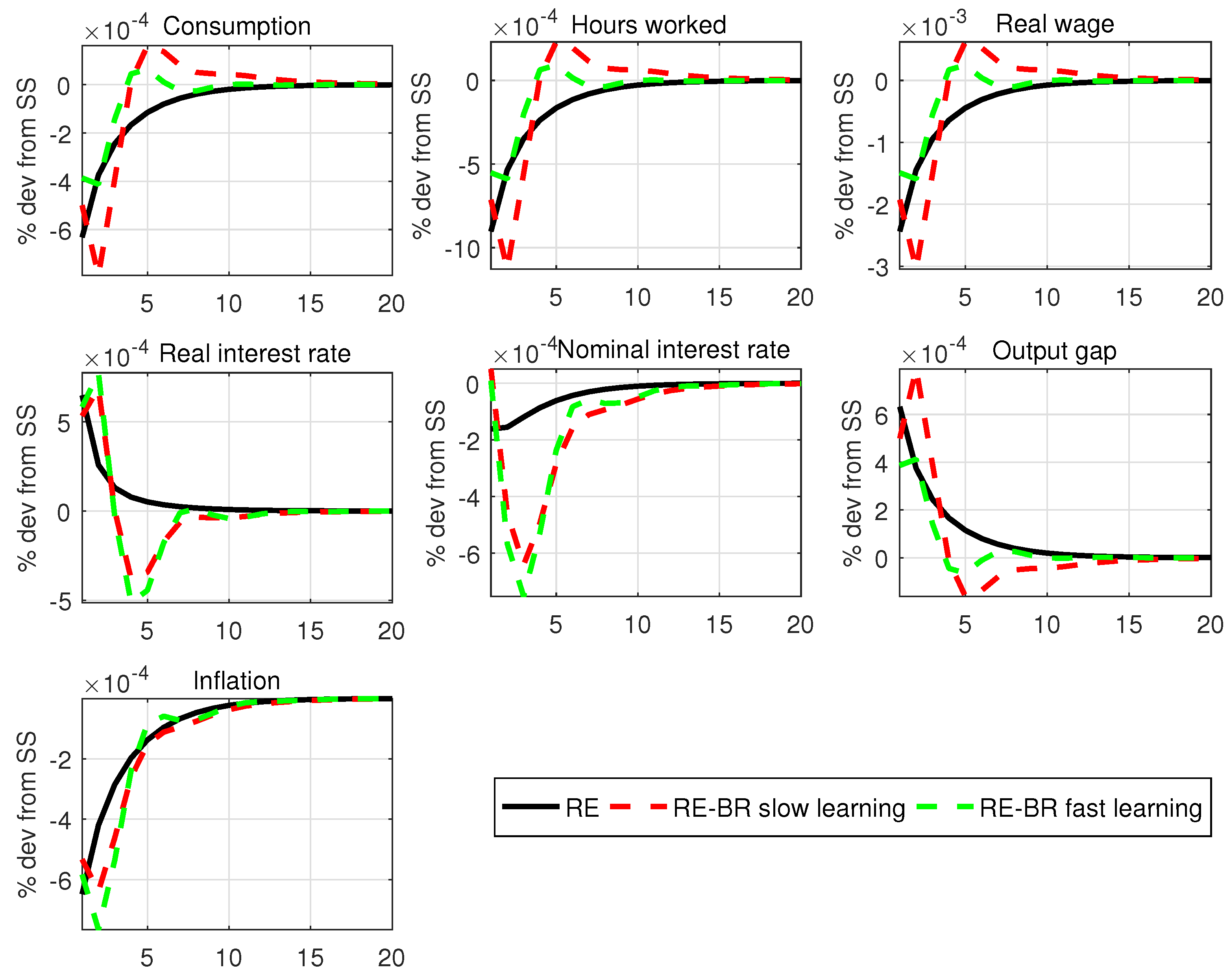
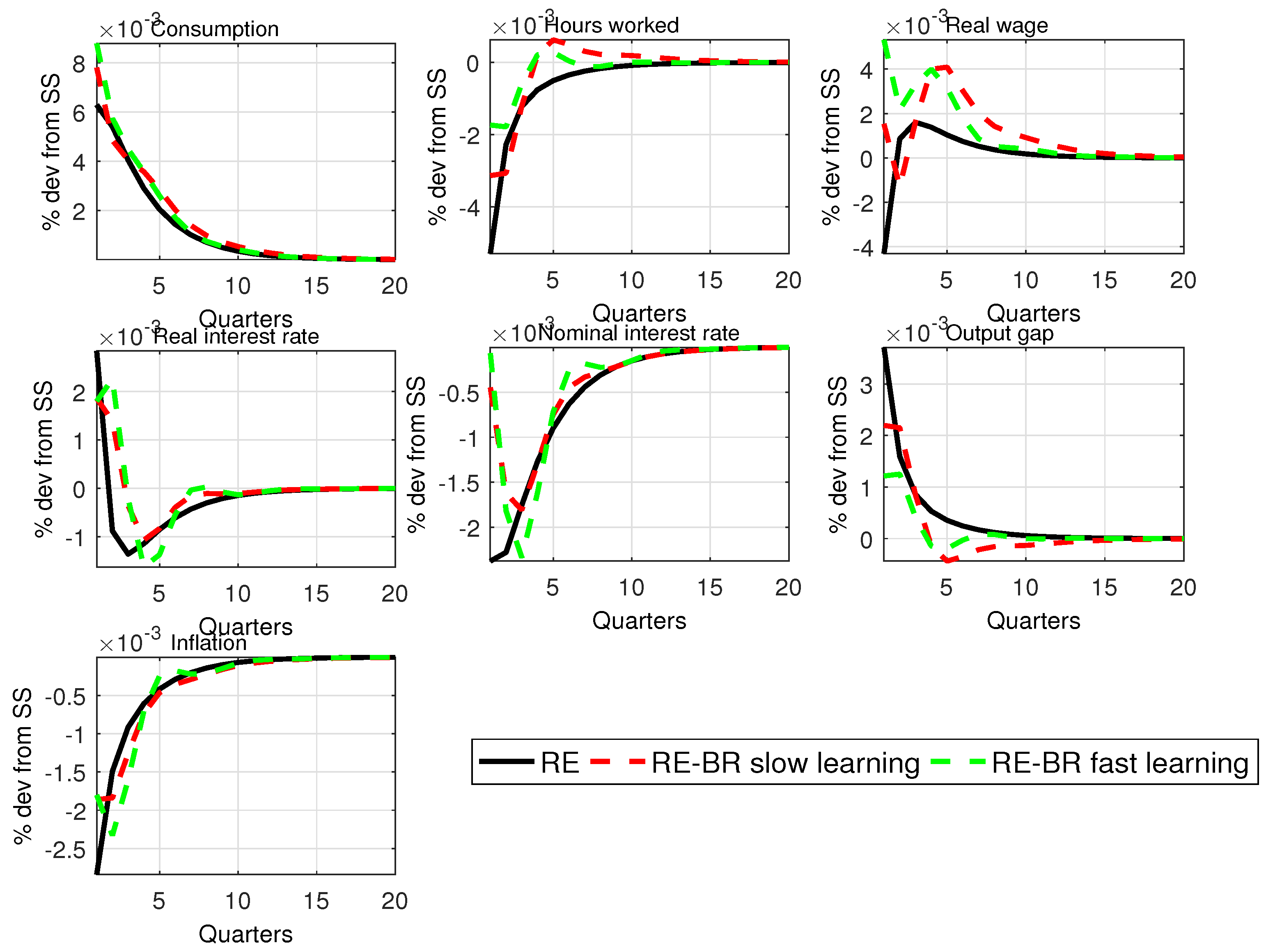
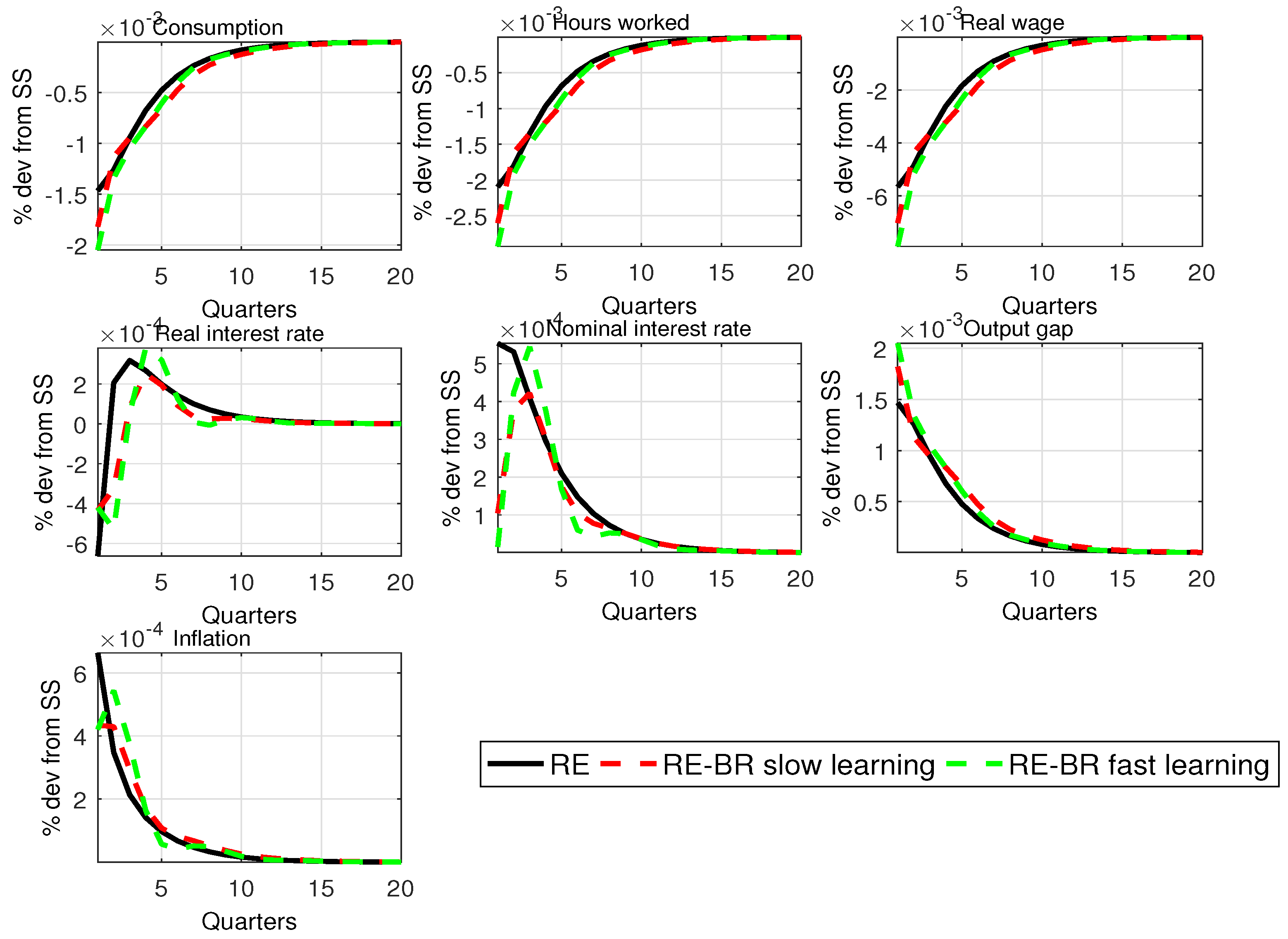
For our model of BR with AU, Figure 1 plots the impulse response functions (IRFs) with standard parameters for the rule for a shock to monetary policy under fast and slow learning. Figure A3 and Figure A4 in Appendix F show IRFs for the technology and mark-up shocks. Not surprisingly, fast learning sees an IRF converge faster to the RE case, but in either case, BR introduces more persistence compared with RE. This suggests that this feature should lead to a better fit of the data without relying on other persistence mechanisms (shocks, habit or price indexing). The stability properties of the model are examined in the WP version of the paper and Appendix A.

5.2. Endogenous Proportions of RE and BR Agents with Reinforcement Learning

Proportions of rational households ($n_{h,t}$) and firms ($n_{f,t}$) are given by (8)

$$n_{j,t}=\frac{exp(-\gamma {\Phi }_{j,t}^{RE})}{exp{(-\gamma {\Phi }_{j,t})}^{RE}+exp(-\gamma {\Phi }_{j,t}^{BR})};j=h,f$$

where fitness for households and firms $j=h,f$ is given by

$$\begin{array}{ccc}\hfill {\Phi }_{j,t}^{RE}& =& {\mu }_j^{RE}{\Phi }_{j,t-1}^{RE}+(1-{\mu }_j^{RE})\left(\mathrm{weighted}\mathrm{sum}\mathrm{of}\mathrm{forecast}\mathrm{errors}+C_j\right)\hfill \\ \hfill {\Phi }_{j,t}^{BR}& =& {\mu }_j^{BR}{\Phi }_{j,t-1}^{BR}+(1-{\mu }_j^{BR})\left(\mathrm{weighted}\mathrm{sum}\mathrm{of}\mathrm{forecast}\mathrm{errors}\right)\hfill \end{array}$$

Table 1. Third-order solution of the estimated NK RE-BR model; ${\mu }_h^{RE}={\mu }_h^{BR}={\mu }_f^{RE}={\mu }_f^{BR}=0$; $\gamma =1,100,1000$.

Variable	Stochastic Mean	Standard Deviation (%)	Skewness	Kurtosis
$\frac{C_t}{C}$	0.999544	0.042057	0.323304	0.093034
$\frac{H_t}{H}$	1.000273	0.005111	0.038002	−0.020743
$\frac{W_t}{W}$	0.999810	0.038145	0.318586	0.073488
$\frac{{\Pi }_t}{\Pi }$	0.999898	0.004235	−0.045800	0.030136
$\frac{R_{n,t}}{R_n}$	0.999887	0.004440	−0.046254	0.044145
${\Phi }_{h,t}^{RE}-C_h$	−0.000443	0.000446	−2.078809	6.635580
${\Phi }_{h,t}^{AE}$	−0.000526	0.000516	−2.168947	8.000489
${\Phi }_{f,t}^{RE}-C_f$	−0.000199	0.000203	−2.279557	9.082031
${\Phi }_{f,t}^{AE}$	−0.000349	0.000342	−2.269953	9.937975
$n_{h,t}(\gamma =1;\sigma =1)$	0.100008	0.000023	0.857638	4.454288
$n_{f,t}(\gamma =1;\sigma =1)$	0.100014	0.000025	1.586194	6.015115
$n_{h,t}(\gamma =100;\sigma =1)$	0.100750	0.002297	0.857638	4.454288
$n_{f,t}(\gamma =100;\sigma =1)$	0.101352	0.002479	1.586194	6.015115
$n_{h,t}(\gamma =1000;\sigma =1)$	0.107501	0.022973	0.857638	4.454288
$n_{f,t}(\gamma =1000;\sigma =1)$	0.113518	0.024787	1.586194	6.015115
$n_{h,t}(\gamma =1000;\sigma =2)$	0.130007	0.093482	0.888592	4.857691
$n_{f,t}(\gamma =1000;\sigma =2)$	0.154182	0.100265	1.683430	6.867599

provides a third-order perturbation solution of the non-linear NK RE-BR model. We use the Bayesian estimation of the model in Reference [30] where the model is linearised and the proportions $n_{h,t}$ and $n_{f,t}$ are fixed. Non-linear estimation would be required to pin down the parameters $n_h$, $n_f$ in the steady state in the BR scenarios and ${\mu }_h^{RE,BR}$, ${\mu }_f^{RE,BR}$ and $\gamma$ in the reinforcement learning process, which goes beyond the scope of this paper. Thus, here we impose them as reported in the table ($n_{h,t}=n_{f,t}=0.1$). We also scale the estimated standard deviations of the shocks using a parameter $\sigma =1,2$. For the robustness of our results, we perform additional simulations, for different choice of the memory parameters, and present the results with ${\mu }_h^{RE}={\mu }_h^{BR}={\mu }_f^{RE}={\mu }_f^{BR}=0.5$ and $=0.75$ in Appendix G. The robustness exercise assumes instead that agents have some memory of past observations.

The main results from these simulations are as follows. First, reinforcement learning introduces high kurtosis and skewness in macroeconomic variables, the absence of kurtosis in the standard NK model, often highlighted in the literature (see, for example, Reference [3]), is in part simply the consequence of linearisation, and non-normality is a feature of higher order approximations. Second, reinforcement learning with stronger switching processes (i.e., $\gamma =100,1000$) coupled with higher volatility of exogenous shocks results in the numbers of rational agents increasing from the estimated deterministic steady state value of $0.1$ to $0.13$ and $0.15$ for households and firms, respectively, in the stochastic steady state. Third, given that BR is a welfare-reducing friction in these models, it follows that volatility can actually be welfare-increasing in our heterogeneous expectations setting. Furthermore, when we assume that agents have some memory of past observations when revising their expectations given their forecast performances, the simulated skewness and kurtosis are lower compared to the case when no memory is assumed in the learning process.

Our main results clearly suggest that, when the switching process between groups of heterogeneous agents becomes more deterministic depending on agents’ willingness to learn from the past performance when predicting future outcomes, this leads to an increase in the level of rationality in the BR macroeconomy. This result is in line with the finding in Reference [3]. The cognitive effect of this selection mechanism is much stronger with the occurrence of large exogenous shocks. This group behaviour not only plays a key role in explaining the dynamic properties of the data, revaluating the importance of expectations in driving economic fluctuations in the spirit of Keynes’ concept of animal spirits, but has important implications for the optimal control of policy in the spirit of the Lucas critique. Depending on intentions on the part of policymakers, the model suggests that different versions of policy can be designed and devised in a game between policymakers and the economy, with uncertainty as to which expectation formation is selected.

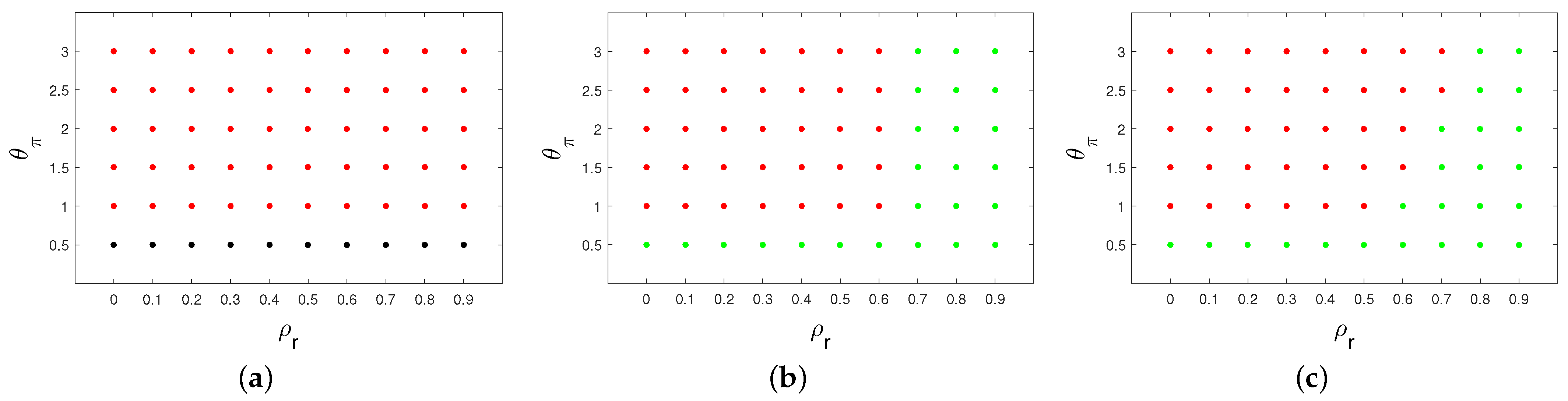
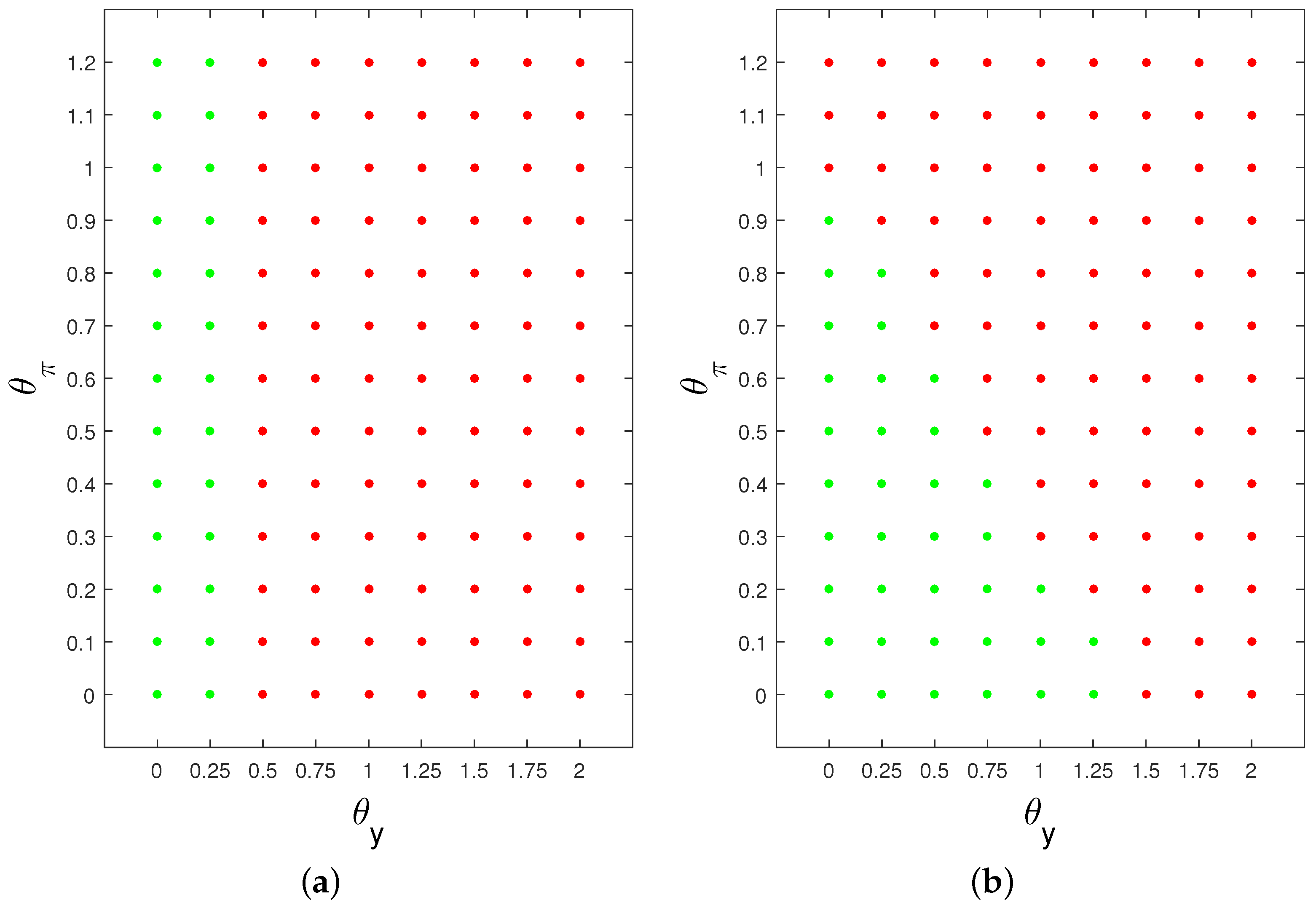
5.3. The Possibility of Bifurcation and Chaotic Dynamics

Non-linear models in general open up the possibility that, for certain parameter values or initial conditions, they may exhibit chaotic dynamics. How are the obtained results related to such dynamics? This possibility is examined using the model of this paper in Reference [22].

The conclusions are: first, the RE determinancy condition for the linearised model in the vicinity of the deterministic steady state ensures local determinancy and stability in the model with a fixed proportion n of fully rational agents. Second, if the linear form of the model starts from a position of indeterminacy, an increase in the fixed cost of being fully rational can lead to the loss of local stability via a Hopf bifurcation. This Hopf bifurcation appears to be super-critical, giving rise to stable limit cycles. As the speed at which agents learn increases, a rational route to randomness appears to follow, which we explore with numerical methods. From a policy point of view, the main conclusion is that local indeterminacy about the steady state can be avoided by a careful choice of interest-rate rule that obeys a “Taylor condition” modified to allow for persistence. This is the case for our simulations which avoid chaotic dynamics.

6. Conclusions

This paper studies an NK behavioural model for which boundedly rational beliefs of economic agents are about payoff-relevant macroeconomic variables that are exogenous to their decision rules. Reinforcement learning is at the core of the heterogeneous expectations model and leads to the striking result that a high volatility of exogenous shocks, by assisting the learning process, can be welfare-increasing.

The results from our simulations have a range of practical and theoretical implications. From a practical point of view, our model provides a behavioural explanation for the important properties of the business cycle dynamics and (ir)rationality under market economy. Our findings shed more light on the underlying mechanism that guides policy choices in a society comprising policymakers and agents who form heterogeneous expectations. Regarding the theoretical implications, our results for a simple NK model suggest a new agenda for constructing empirical medium-sized NK models for agents’ behaviours under imperfect information. Future work will embed the RE-BR composite model into a richer NK macroeconomic model along the lines of Reference [31], use non-linear estimation methods to identify a number of parameters involving reinforcement learning that are not identified using linear Bayesian estimation, and examine optimal monetary policy.

Another potential direction for future research is to investigate how reinforcement learning affects the possible chaotic dynamics of the model. We know that an increase in the fixed cost of being fully rational can lead to the loss of local stability. If we enter a region of local instability, but global boundedness, we see chaotic dynamics as highlighted generally in Reference [25]. In addition, from Reference [22], who plotted the simulated trajectories for various parameter values with an almost purely stochastic switching process ($\gamma =0.1$), it is evident that, when the level of rationality varies according to reinforcement learning, it is likely that we see very different stability/determinancy properties of the model, which imply that uncertainty as to how expectations and learning are processed can lead to a policy rule that is unstable or has infinite multiple equilibria (i.e., is indeterminate).

As with any research, there are limitations in our study that should be addressed in future work. We have alluded to the wilderness of non-rational expectations posed by the sheer size of the literature on behavioural macroeconomics and the huge number of equilibria proposed. Any analysis based on only one choice of model clearly has limitations when turning to policy implications. A policy that works well for one particular choice may perform badly using a different model. One solution to this problem proposed by References [32,33] is to choose a policy to maximise weighted average inter-temporal welfare across a set of competing models and to weigh models based on relative forecasting performance. In other studies, the proportions of rational and non-rational agents are fixed; a possible avenue for future research would be to extend the analysis to time-varying endogenous proportions as in this paper.

Finally, there remains a wide range of views over the asymmetric macroeconomic effects of economic shocks (e.g., news, energy and monetary policy) as well as over the variations in these effects with respect to economic conditions and states. Different strands of literature offer different explanations on the existence of non-linearities, focusing on the sources of the shocks, econometric specifications and time-variation in impact and policy responses (see Reference [34] for a recent study that addresses the latter two aspects). We argue that the modelling approach and non-linear techniques used in our paper add an important dimension to this strand of literature by providing a variety of starting points for future work that investigates the non-linear effects of shocks that may originate from the time-varying nature of expectation formations and complex adaptive systems.

References

1. Branch, W.A.; Evans, G.W. Monetary Policy and Heterogeneous Agents. Econ. Theory 2011, 47, 365–393. [Google Scholar] [CrossRef]
2. De Grauwe, P. Animal spirits and monetary policy. Econ. Theory 2011, 47, 423–457. [Google Scholar] [CrossRef]
3. De Grauwe, P. Booms and Busts in Economic Activity: A Behavioral Explanation. J. Econ. Behav. Organ. 2012, 83, 484–501. [Google Scholar] [CrossRef]
4. De Grauwe, P. Lectures on Behavioral Macroeconomics; Princeton University Press: Princeton, NJ, USA, 2012. [Google Scholar]
5. Sims, C. Macroeconomics and Reality. Econometrica 1980, 48, 1–48. [Google Scholar] [CrossRef]
6. Evans, G.W.; Honkapohja, S. Learning and Macroeconomics. Annu. Rev. Econ. 2009, 1, 421–449. [Google Scholar] [CrossRef]
7. Eusepi, S.; Preston, B. The science of monetary policy: An imperfect knowledge perspective. In Federal Reserve Bank of New York Satff Reports; No. 782; Federal Reserve Bank of New York: New York, NY, USA, 2016. [Google Scholar]
8. Branch, W.A.; McGough, B. Heterogeneous Expectations and Micro-Foundations in Macroeconomics. In Handbook of Computational Economics 4; Elsevier: Amsterdam, The Netherlands, 2018. [Google Scholar]
9. CalvertJump, R.; Levine, P. Behavioural New Keynesian Models. J. Macroecon. 2019, 59, 58–77. [Google Scholar]
10. Caiani, A.; Godin, A.; Caverzasi, E.; Gallegati, M.; Kinsella, S.; Stiglitz, J. Agent based-stock flow consistent macroeconomics: Towards a benchmark model. J. Econ. Dyn. Control 2016, 69, 375–408. [Google Scholar] [CrossRef]
11. Tesfatsion, L. Agent-based computational economics: A constructive approach to economic theory. In Handbook of Computational Economics; Tesfatsion, L.S., Judd, K.L., Eds.; North-Holand: Amsterdam, The Netherlands, 2006; pp. 831–880. [Google Scholar]
12. Levine, P. The State of DSGE Modelling. In Oxford Research Encyclopedia of Economics and Finance; Oxford University Press: Oxford, UK, 2020. [Google Scholar]
13. Brock, W.A.; Hommes, C. A Rational Route to Randomness. Econometrica 1997, 65, 1059–1095. [Google Scholar] [CrossRef]
14. Tamvada, J.P.; Chowdhury, R. The irrationality of rationality in market economics: A paradox of incentives perspective. Bus. Soc. 2023, 62, 482–487. [Google Scholar] [CrossRef]
15. Sirota, M.; Juanchich, M.; Holford, D.L. Rationally irrational: When people do not correct their reasoning errors even if they could. J. Exp. Psychol. Gen. 2023. advance online publication. [Google Scholar] [CrossRef]
16. Kreps, D. Anticipated Utility and Dynamic Choice. In Frontiers of Research in Economic Theory; Jacobs, D., Kalai, E., Kamien, M., Eds.; Cambridge University Press: Cambridge, UK, 1998; pp. 242–274. [Google Scholar]
17. Adam, K.; Marcet, A. Internal Rationality, Imperfect Market Knowledge and Asset Prices. J. Econ. Theory 2011, 146, 1224–1252. [Google Scholar] [CrossRef]
18. Cogley, T.; Sargent, T.J. Anticipated utility and rational expectations as approximations of bayesian decision making. Int. Econ. Rev. 2008, 49, 185–221. [Google Scholar] [CrossRef]
19. Branch, W.A.; McGough, B. Dynamic predictor election in a new keynesian model with heterogeneous agents. J. Econ. Dyn. Control 2010, 34, 1492–1508. [Google Scholar] [CrossRef]
20. Massaro, D. Heterogeneous Expectations in Monetary DSGE Models. J. Econ. Dyn. Control 2013, 37, 680–692. [Google Scholar] [CrossRef]
21. Cornea-Madeira, A.; Hommes, C.; Massaro, D. Behavioral Heterogeneity in U.S. Inflation Dynamics. J. Bus. Econ. Stat. 2019, 37, 288–300. [Google Scholar] [CrossRef]
22. CalvertJump, R.; Hommes, C.; Levine, P. Learning, Heterogeneity, and Complexity in the New Keynesian model. J. Econ. Behav. Organ. 2019, 166, 446–470. [Google Scholar] [CrossRef]
23. Milani, F. Expectations, learning and macroeconomic persistence. J. Monet. Econ. 2007, 54, 2065–2082. [Google Scholar] [CrossRef]
24. Anufriev, M.; Hommes, C.; Makarewicz, T. Simple Forecasting Heuristics that Make Us Smart: Evidence from Different Market Experiments; Working Paper Series 29; Economics Discipline Group, UTS Business School, University of Technology: Sydney, Australia, 2015. [Google Scholar]
25. Hommes, C. Behavioral Rationality and Heterogeneous Expectations in Complex Economic Systems; Cambridge University Press: Cambridge, UK, 2013. [Google Scholar]
26. Schmitt-Grohe, S.; Uribe, M. Closing small open economy models. J. Int. Econ. 2003, 61, 163–185. [Google Scholar] [CrossRef]
27. Dixit, A.K.; Stiglitz, J.E. Monopolistic competition and optimal product diversity. Am. Econ. Rev. 1977, 67, 297–308. [Google Scholar]
28. Calvo, G. Staggered Prices in a Utility-Maximising Framework. J. Monet. Econ. 1983, 12, 383–398. [Google Scholar] [CrossRef]
29. Nimark, K.P. Man-Bites-Dog Business Cycles. Am. Econ. Rev. 2014, 104, 2320–2367. [Google Scholar] [CrossRef]
30. Deak, S.; Levine, P.; Pearlman, J.; Yang, B. Internal Rationality, Learning and Imperfect Information; School of Economics, University of Surrey: Guildford, UK, 2017; Discussion Papers 08/17. [Google Scholar]
31. Smets, F.; Wouters, R. Shocks and Frictions in US business cycles: A Bayesian DSGE approach. Am. Econ. Rev. 2007, 97, 586–606. [Google Scholar] [CrossRef]
32. Deak, S.; Mirza, A.; Levine, P.; Pearlman, J. Designing Robust Policies using Optimal Pooling; School of Economics, University of Surrey: Guildford, UK, 2019; Discussion Papers 12/19. [Google Scholar]
33. Deak, S.; Mirza, A.; Levine, P.; Pham, S. Negotiating the Wilderness of Bounded Rationality through Robust Policy; School of Economics, University of Surrey: Guildford, UK, 2023; Discussion Papers 02/23. [Google Scholar]
34. Bildirici, M.; Ersin, O. Markov-switching vector autoregressive neural networks and sensitivity analysis of environment, economic growth and petrol prices. Environ. Sci. Pollut. Res. 2018, 25, 31630–31655. [Google Scholar] [CrossRef] [PubMed]
Figure 1. RE versus RE-BR composite expectations with n h = n f = 0.5 , λ x = 0.25 , 1.0 ; Taylor rule with ρ r = 0.7 , θ π = 1.5 and θ y = 0.3 , θ d y = 0 ; monetary policy shock.
Algorithms 16 00280 g001