
Cathode Shape Design for Steady-State Electrochemical Machining


Lehrstuhl für Werkstoffkunde und Werkstoffmechanik, Technische Universität München, Boltzmannstraße 15, 85748 Garching, Germany
*
Author to whom correspondence should be addressed.
Algorithms 2023, 16(2), 67; https://doi.org/10.3390/a16020067
Submission received: 19 December 2022
/
Revised: 14 January 2023
/
Accepted: 16 January 2023
/
Published: 19 January 2023
(This article belongs to the Collection Feature Papers in Algorithms)
Abstract
:The inverse or cathode shape design problem of electrochemical machining (ECM) deals with the computation of the shape of the tool cathode required for producing a workpiece anode of a desired shape. This work applied the complex variable method and the continuous adjoint-based shape optimization method to solve the steady-state cathode shape design problem with anode shapes of different smoothnesses. An exact solution to the cathode shape design problem is proven to exist only in cases when the function describing the anode shape is analytic. The solution’s physical realizability is shown to depend on the aspect ratio of features on the anode surface and the width of the standard equilibrium front gap. In cases where an exact and physically realizable cathode shape exists, the continuous adjoint-based shape optimization method is shown to produce accurate numerical solutions; otherwise, the method produces cathode shapes with singularities. For the latter cases, the work demonstrates how perimeter regularization can be applied to compute smooth approximate cathode shapes suitable for producing workpieces within the range of manufacturing tolerance.
1. Introduction
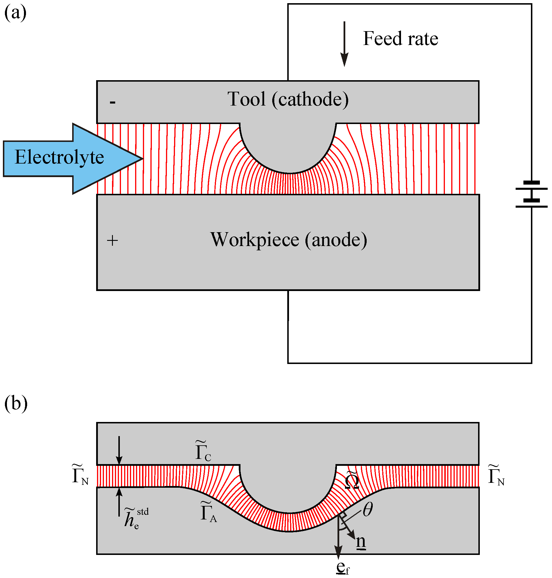
Electrochemical machining (ECM) is a non-conventional machining technique. Its principle is shown in Figure 1. Since it is contactless, ECM can be applied in the manufacturing of complex-shaped parts made of high-strength materials without introducing residual stresses into the workpiece and without tool wear. Today, applications of ECM include the production of turbine disks and blades in aerospace industry [1,2], manufacturing of fuel injection devices in automotive industry [3], production of gun barrels in weapon industry [4], fabrication of medical implants [5], or shaping three-dimensional (3D) structures with submicrometer precision [6]. An overview of the recent developments of ECM is presented in review articles [2,7].
One of the main disadvantages of ECM is the long production preparation cycle, especially for the tool cathode that is required for producing workpieces of complex shapes. In this context, two problems exist: the direct- or anode shape prediction problem of ECM refers to anticipating the evolution of the anode shape in a defined standard ECM process with a given set of process parameters and a known shape of the cathode. In industrial applications, however, the known information is often the desired shape of the workpiece, resulting in a problem that is referred to as the inverse- or cathode shape design problem of ECM.
Regarding the solution of the direct problem, the main focus is—apart from the prediction of the anode shape—on modeling different interdependent physical and chemical processes within the interelectrode gap during machining. The results of numerous studies are summarized in a comprehensive review [9]. In recent years, the focus has been turned to verifying multiphysics models with experiments [10], or taking further processes such as short pulses [11], electrochemical reaction kinetics [12], or the mechanical oscillation of the cathode [13] into account. Recently, machine learning techniques have been applied to predict workpiece profiles after ECM [14] or the microstructure and mechanical properties of materials [15,16,17].
Due to the relevance for industrial applications, numerous researchers have developed algorithms for solving the inverse or cathode shape design problem. These methods can be classified into the following groups:
- Approximative analytical methods: Tipton [18] proposed the so-called -method, assuming the width of the interelectrode gap to be inversely proportional to , where is the angle between the normal of the local anode surface and the cathode feed direction (see Figure 1b). However, this method is only applicable in gap regions where is less than [19].
- Exact analytical methods: The complex variable method applied by Krylov [20], Nilson and Tsuei [21], and extended by Alder et al. [22] makes use of the harmonic property of holomorphic functions and the principle of analytic continuation. However, due to the number of degrees of freedom in the complex plane, this method is inherently limited to 2D applications.
- Numerically solving an “initial value problem”: Some authors solve the cathode shape design problem either via computing a solution to a system of ordinary differential equations [23] or by imposing both anode boundary conditions on the finite element discretized equation [24,25,26]. These methods, especially the latter, require a non-standard numerical scheme different from those used when solving conventional boundary value problems of partial differential equations. Furthermore, the method of Zhu et al. [24] and Sun et al. [25] is assumed to only be applicable to electrode shapes with gentle curvatures [9].
- Correction methods: Reddy et al. [27] proposed a correction factor method that makes local corrections of the cathode shape based on the shape of the anode obtained as the numerical solution to the direct problem. The underlying ECM model extends the potential model by taking into account a variable electrolyte conductivity that depends on the temperature and void fraction distribution within the electrolyte [19,28,29,30]. The correction factor method was included in an integrated tool design approach described by Jain and Rajurkar [31]. Narayanan et al. [32] and Hardisty and Mileham [33] corrected the shape of the cathode based on the deviation of the current density on the anode. In several studies, correction methods for cathode shape design are proposed, taking multiphysics ECM models into account [34,35,36,37]. Correction methods have a wide field of use, including cathode shape design for non-steady-state ECM, such as electrochemical drilling [27] or electrochemical trepanning [37]. For these methods, much numerical expertise and effort are required to develop a computational environment.
- Embedding method: Hunt [38] approximated the shape of the cathode, computed anode, and required anode by sums of basis functions and computed the shape of the cathode by solving a nonlinear equation system for the corresponding coefficients (i.e., the design variables of the cathode). The method was applied by Chang and Hourng [39] to solve the cathode shape design problem in two dimensions, taking multiphase flow into account. Since the solution of the nonlinear equation system involves the computation of the Jacobian for the Newton method, the anode shape prediction problem has to be solved times per iteration (M is the number of coefficients), making the method computationally expensive.
- Optimization methods: Several approaches approximate the shape of the cathode, computed anode, and required anode by sums of basis functions and use gradient-based minimization of an objective function to compute the coefficients of electrode shape basis functions [39,40,41]. However, the approaches are also computationally expensive and require the anode shape prediction problem to be solved times per iteration. This work applied the continuous adjoint shape optimization method that is capable of solving the steady-state cathode shape design problem in three dimensions [8]. The method is efficient since only two Laplace equations per optimization iteration have to be solved, although the number of design variables M corresponds to the degree of freedom of the mesh nodes at the cathode surface. In addition, key steps of the method only involve solving the Laplace equation or computing normal derivatives of computed scalar fields at boundaries. These are standard routines in many commercial or open-source simulation tools, making the method also accessible for a larger group of application engineers who are not directly related to research since there is no need to implement complex solvers or algorithms for numerical computations from scratch.
Regardless of the solution approach, and even in the simplest case of the potential model, the cathode shape design problem is a free-boundary Cauchy problem of the Laplace equation, which is known to be ill-posed [42]. For these problems, small changes in the given data may cause large changes in the solution, which is a challenge, especially for numerical computations.
In this work, we applied the complex variable method [20,21,22] and the continuous adjoint-based shape optimization method [8] to answer the following questions:
- What are the conditions for the existence of an exact and physically realizable cathode shape?
- How does the solution computed using the continuous adjoint-based shape optimization method behave depending on the existence of an exact and physically realizable cathode shape?
- How can the ill-posed nature be “overcome” in the sense of computing an acceptable approximate solution to the cathode shape design problem in practical engineering cases?
2. Fundamentals and Methods
2.1. Modeling the ECM Process
Due to the large number of interdependent process variables, multiphysics models are required to describe the general ECM process. For simplification, the major part of this work uses the so-called potential model [41,43,44,45] as the underlying ECM process model. Within this model, the primary electric current distribution is considered, which is a function of the applied voltage, the electrolyte conductivity, and the gap geometry only [46]. The change in the geometry of the interelectrode gap due to material dissolution at the anode surface results in a change in the current density, which, in turn, affects the local rate of material dissolution. As shown by experiments (see Appendix A), the potential model can describe the ECM process under ideal conditions.
The mathematical formulation of the potential model (cf. Lu et al. [8], Equations (1)–(4)) can be nondimensionalized by normalizing spacial quantities to the standard equilibrium front gap width and the electric potential to the effective voltage across the interelectrode gap. The dimensionless electric potential within the interelectrode gap is computed by solving the equations
where is the computational domain covering the interelectrode gap, and , , and denote the non-metallic side boundaries, the cathode surface boundary, and the anode surface boundary, respectively (see Figure 1b).
2.2. Steady-State Anode Shape Prediction
In this work, the direct problem of ECM is solved numerically. The solution is used mainly to verify the quality of the computed cathode shapes as the solution to the inverse problem. Since only the steady-state anode shape is of interest, the machining process can be considered in a reference coordinate frame tied to the cathode. In this frame, the cathode boundary is fixed, and the velocity of the anode boundary is given by , where denotes the dissolution velocity and is the unit vector in the feed direction (usually pointing to the negative z-direction of the coordinate system). Since only the velocity component normal to the boundary leads to a change in the shape of the gap domain, the velocity of the anode boundary is replaced by its normal component, i.e.,
In the beginning of each simulation time step, the electric potential is computed by solving the finite-volume-discretized form of Equations (1)–(4) using libraries of the open-source C++ toolbox OpenFOAM® (“Open-source Field Operation And Manipulation”). The central-difference scheme is applied to obtain the flux at the control volume faces, as proposed for steady-state heat conduction problems (see [47], Chapter 4). The conjugate gradient method is applied to solve the resulting linear equation system with a symmetric coefficient matrix. Then, the dimensionless anode shape change velocity is evaluated according to Equation (5). Before the next simulation time step starts, the anode boundary motion velocity is propagated to the interior of the mesh by the approach described by Löhner and Yang [48] and the mesh is updated. The computations of this work were carried out on a single Intel Xeon X5550 processor (2.67 GHz).
2.3. Cathode Shape Design for Steady-State ECM
In the majority of the examples shown in this work, the inverse problem of ECM is solved numerically by continuous adjoint-based shape optimization aimed at minimizing the (reduced) objective function (cf. [8], Equation (41)):
where denotes the angle between the outer surface normal of the anode surface boundary and the feed direction of the cathode (see Figure 1b). Each iteration starts with solving for the electric potential (Equations (1)–(4)) and for the Lagrange multiplier governed by the adjoint equations (cf. Lu et al. [8], Equations (44)–(47)):
When the domain is deformed infinitesimally into , the change in the reduced objective function is given by the so-called reduced gradient,
To optimize the shape of the cathode by the steepest descent method, each point on is moved according to (cf. [8], Equation (53))
in an iteration step with step length . The numerical schemes and the mesh deformation method are similar to those applied when solving the direct problem. To evaluate the convergence of the optimization process, the maximum of the shape gradient,
and that of the integrand of the shape optimization objective function (Equation (6)),
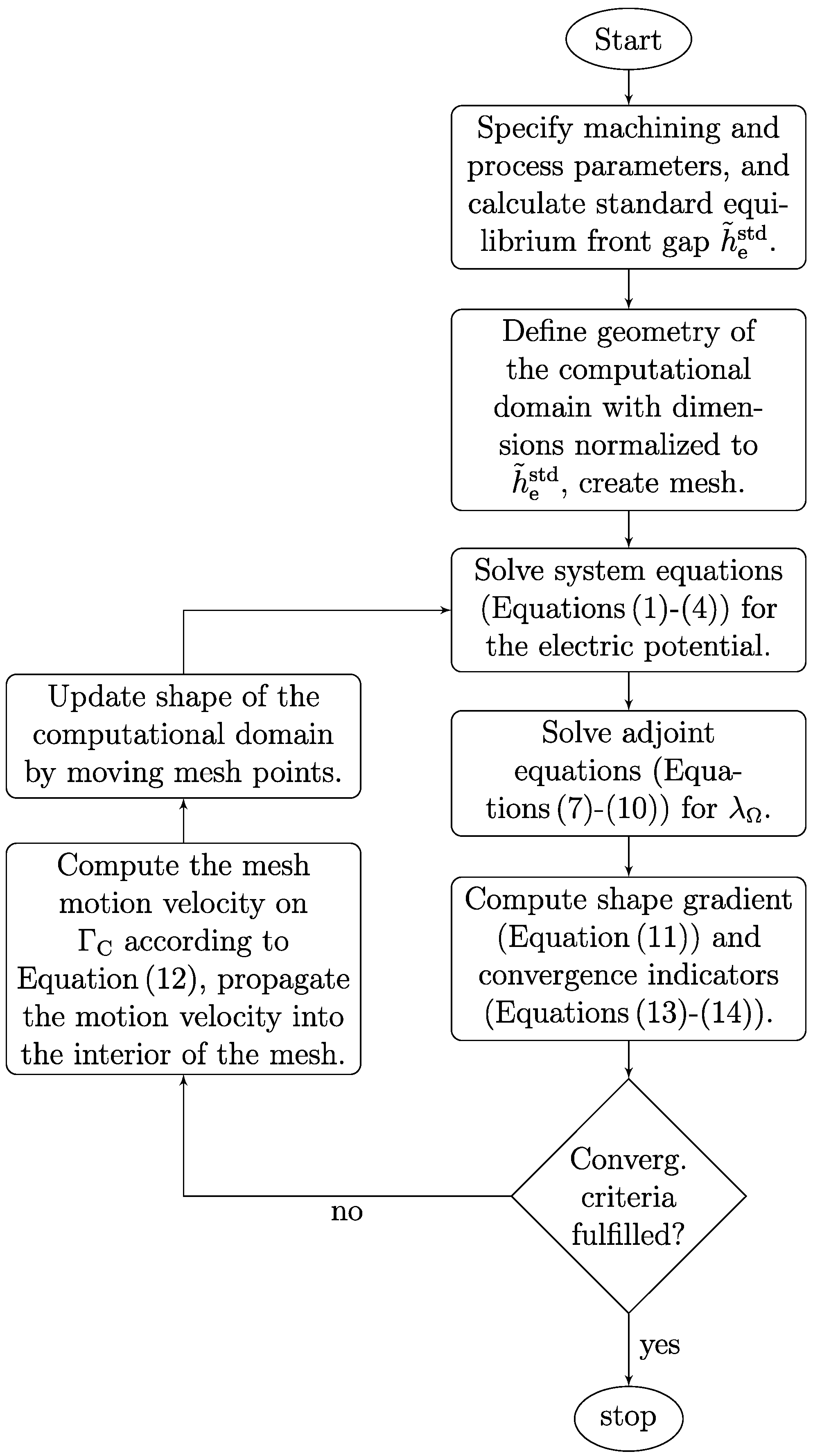
are monitored (cf. [8], Section 3.2.1). A schematic diagram of the cathode shape design procedure is shown in Figure 2.
In certain 2D cathode shape design problems, explicit analytical solutions can be found if the anode shape is analytic, i.e., with an analytic function F. For these cases, the complex variable method [21] is used to calculate the surface profile of the unknown cathode as a curve with parameter in the x-z-plane (cf. [8], Appendix C). The coordinates of the curve points are given by
The complex variable method is used to discuss the existence of solutions in general cases and serves as an additional way to verify numerically computed solutions.
3. Results and Discussion
3.1. Cathode Shape Design for Smooth Anode Shapes
3.1.1. Analytical Solutions
To illustrate the physical realizability of solutions to the cathode shape design problem, anode profiles in the shape of a smooth indentation are modeled by the graph of a Gaussian:
The complex variable method is applied to calculate the required shape of the cathode in the x-z plane, resulting in
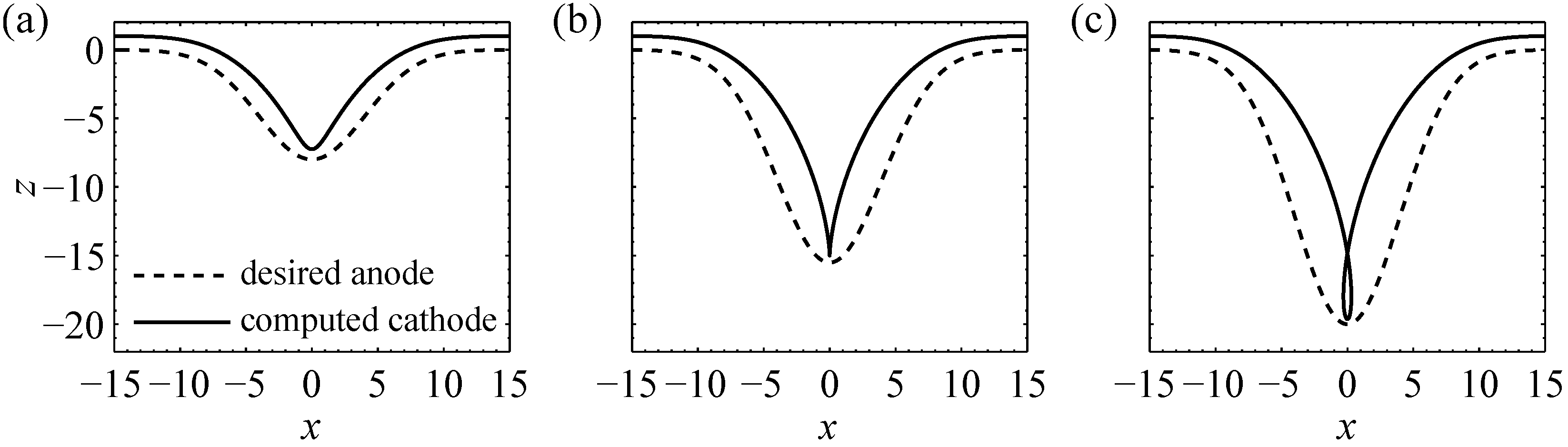
Figure 3 illustrates surface profiles of anodes and the corresponding cathodes obtained for three combinations of the parameters A and . While the shapes of the anodes are smooth in all three panels, the cathodes have qualitatively different shapes, respectively. In Panel (a), the cathode is regular and in line with ECM experience because the cathode is approximately the negative image of the anode. In Panel (c), the cathode surface profile has a “loop” at , which is physically not meaningful as the cathode cannot penetrate itself. The cathode shape in Panel (b) with a singularity at seems to be the limit between physically meaningful (i.e., realizable) and meaningless cathodes.
The qualitative behavior of the cathode shapes in Figure 3 can be understood by considering the derivative of (Equation (18)) with respect to . For , is positive for all , i.e., increases monotonously. For , is negative near , resulting in a physically meaningless loop of the cathode surface profile in Figure 3c. For given width ,
is the maximum amplitude of a Gaussian-shaped anode described by Equation (17), where an exact and physically realizable cathode shape exists.
In cases where the exact shape of the cathode obtained through the complex variable method has “loops” (see, e.g., Figure 3c), it is important to investigate if the numerical approach on the basis of shape optimization yields comparable solutions.
3.1.2. Numerical Computations
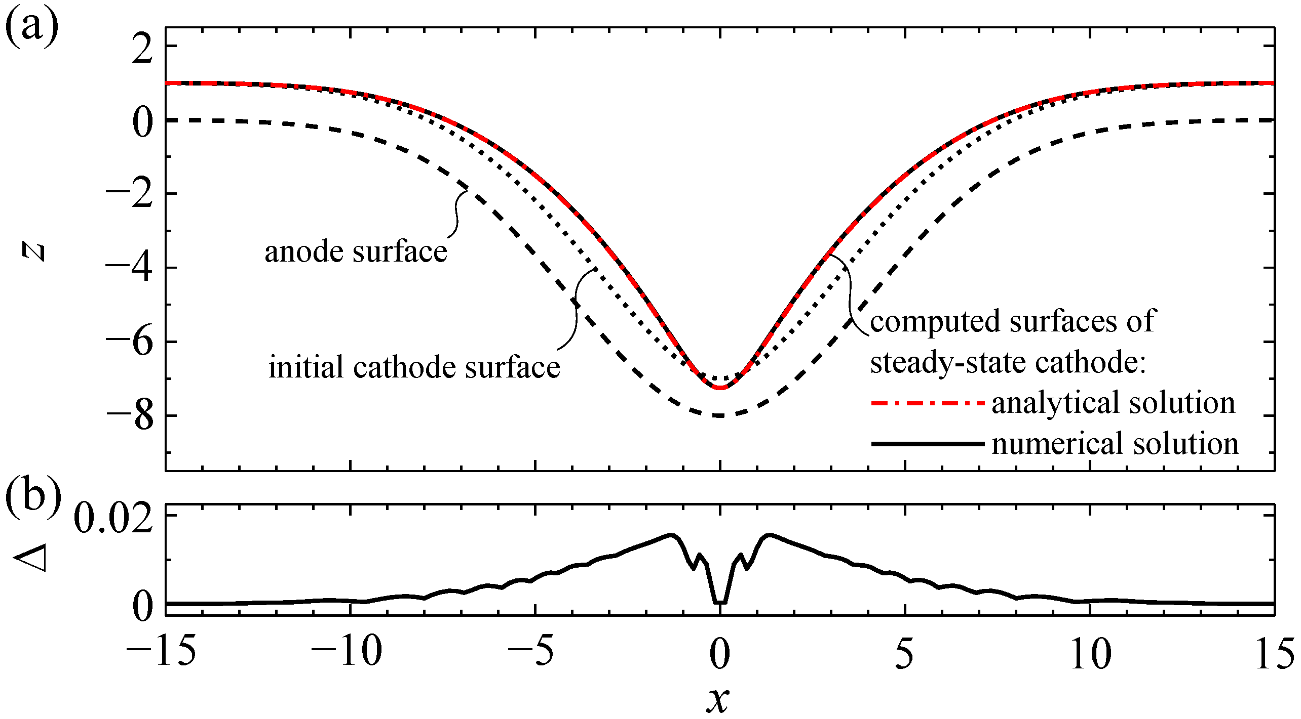
The numerical simulation tool for the cathode shape design was applied to the anode shape defined by Equation (17) with and several values of A. Figure 4 exemplarily illustrates the results for an anode with (black dashed line in Panel (a)), for which, a regular shape of the cathode was obtained in the analytical calculation (cf. Figure 3a). For the iterative computation based on continuous adjoint shape optimization, the offset curve of the anode with a normal distance of 1 (dotted black line in Figure 4a) is assumed to be the surface profile of the initial cathode. The computational domain was discretized by a mesh; the computation was carried out for 200 iteration steps with constant step length (see Equation (12)).
The surface profile of the cathode obtained after 200 iterations is shown by the solid line in Figure 4a, which overlaps with the analytical solution given by Equations (18) and (19) (dash dotted line) on the scale of the figure. For clearer visualization, the absolute deviation between these solutions, measured in surface normal direction, was computed and is shown in Figure 4b. The maximum of , denoted by , is less than , i.e., 2% of the width of the standard steady-state front gap.
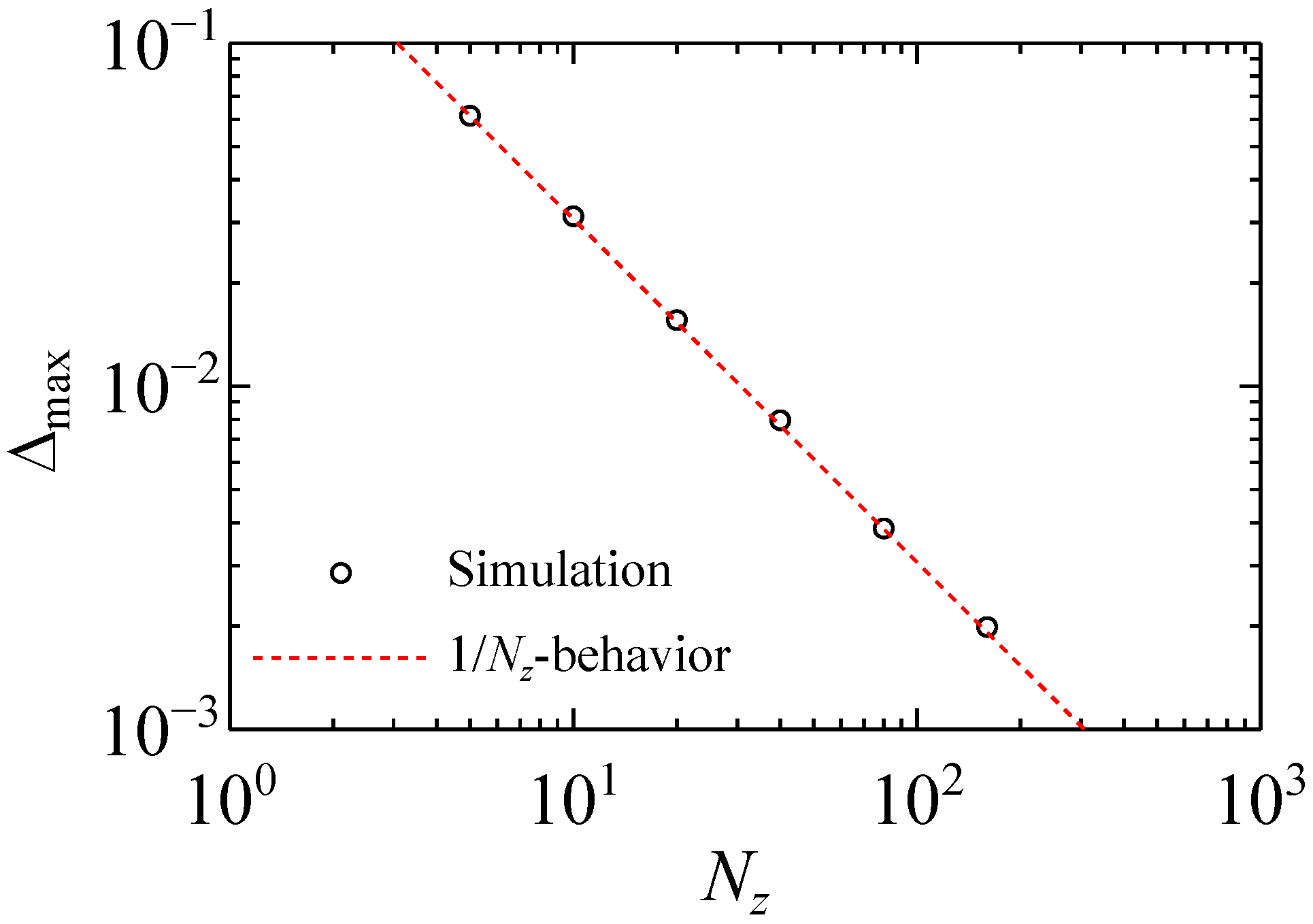
The results of the simulation were also assessed in terms of the mesh dependence of its accuracy. The surface profiles of the anode and the initial cathode remain the same as those shown in Figure 4. The maximum normal deviation () of the numerically obtained cathode shapes from the analytical solution (Equations (18) and (19) was computed in each case.
The computational domain was discretized by meshes. For and varying between 200 and 800, no significant changes in are observed (not displayed). Figure 5 shows the quantity as a function of that ranges from 5 to 160 while is kept fixed. As evident from the figure, is inversely proportional to , indicating an improvement in accuracy due to mesh refinement in the case where the shape of the cathode is regular.
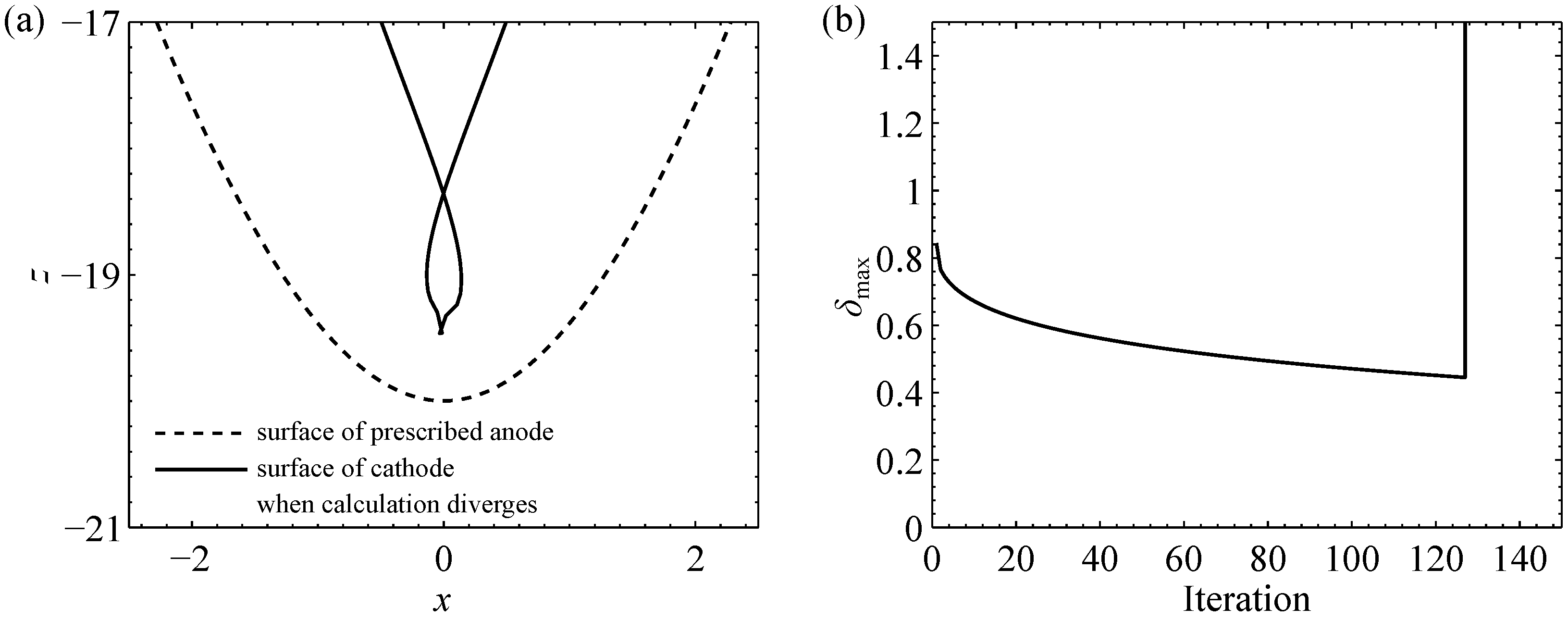
As an example of a case in which a non-physical shape of the cathode was obtained in the analytical calculation (cf. Figure 3c), the numerical computation procedure was applied to an anode shape with and . During the iterative optimization procedure, the cathode boundary forms a loop before the computation diverges due to errors resulting from the degenerated mesh. The solid curve in Figure 6a illustrates the cathode surface profile in the vicinity of the vertex in the last iteration before the computation diverges. Figure 6b shows the evolution of the convergence indicator (Equation (14)).
The loop of the numerically computed cathode surface profile agrees qualitatively with the analytical solution. Quantitatively, the numerically and analytically computed cathode shapes cannot be compared with each other since the numerical computation is stopped before convergence. However, the convergence measure, , decreases with an increasing number of iterations before the error occurs, indicating that the cathode shape in the numerical computation tries to approach the (physically meaningless) analytical solution as long as the mesh is not degenerated.
To interpret the results shown in Figure 3 and Figure 6 in terms of their significance for practice, the critical amplitude of the anode (cf. Equation (20)) has to be expressed in the dimensioned form
where is the standard equilibrium front gap in steady-state condition. According to Equation (21), the dimensioned critical amplitude () increases with a decreasing for a given horizontal dimension of the anode (). Hence, for anode shapes with large ratios of the vertical to horizontal dimension (i.e., ratio) a physically realizable cathode shape only exists if is sufficiently small. The phenomenon that some cathode shapes are physically meaningless has been mentioned by Krylov [20] and Alder et al. [22]; it is not caused by the complex variable method [21] but is a consequence of the nature of the inverse problem. As shown by the example in Figure 6, this conclusion also applies to the failure of the numerical computation.
3.2. Cathode Shape Design for Anode Shapes with Limited Smoothness
3.2.1. Analytical Solutions
For producing an anode whose surface profile is represented by a graph of a continuous but non-analytic function F on an interval , the required shape of the cathode can be calculated using the method proposed by Alder et al. [22]. In this method, F is thought to be continued periodically and approximated by Fourier polynomials
with Fourier coefficients and . Then, the complex variable method is applied to , resulting in
as the parametric representation of the cathode. In the following example, the surface profile of the anode is defined by the continuous function
which has a sharp bend at (see Figure 7) intended to model sharp edges or corners in reality. The approximating Fourier polynomial is given by
With Equations (23) and (24), the surface profile of the cathode required to produce the approximated anode with surface profile is given by the parametric representation
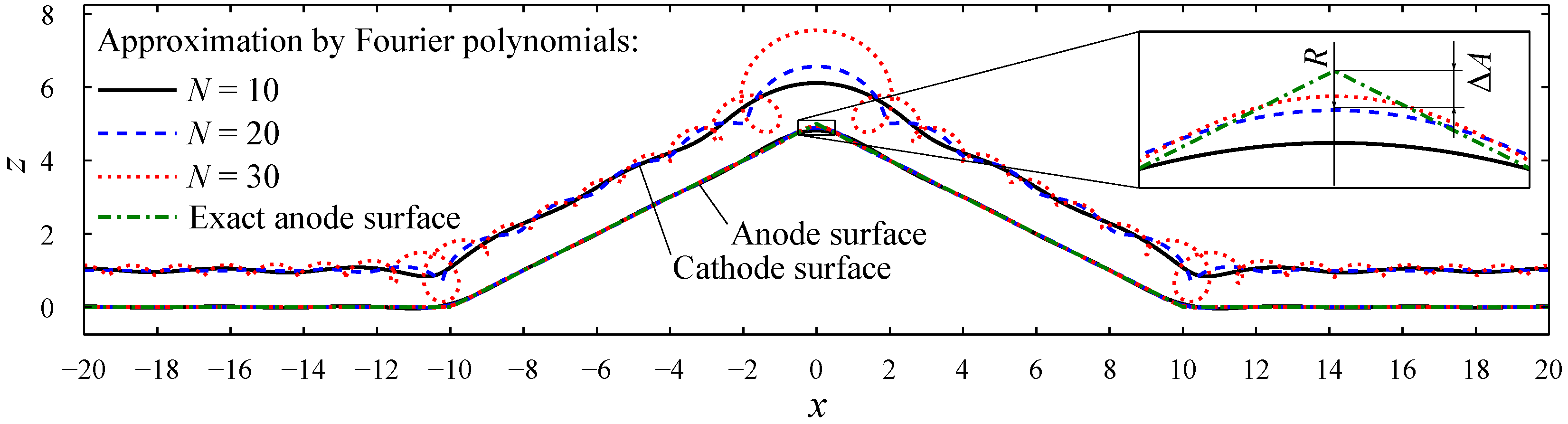
Figure 7 shows examples in which the surface profile of the anode described by Equation (25) with and is approximated by Fourier polynomials (26) of degree , and 30, respectively. The precision of the approximation increases with an increasing N since, for a continuous function F, the function sequence converges uniformly. The maximum deviation of the anode surface profiles and from each other, which is found at , is below ; however, the maximum deviation of the corresponding cathode surface profiles from each other is larger than . Furthermore, with an increasing N, the cathode shape becomes increasingly “distorted”: The cathode surface profile changes from regular (, solid line) over singular (, dashed line) to physically meaningless (, dotted line). The size of the “loops” in the physically unrealizable case increases with a decreasing distance to the sharp bends of the anode surface at and .
The behavior of the cathode shapes shown in Figure 7 can be understood by analyzing the magnitude of the coefficients , , and of the harmonic terms in Equations (26)–(29). For the approximate anode, the coefficients decrease like . For the resulting cathodes, however, the coefficients and increase like and . When the degree N of the Fourier polynomial increases, the approximation of the shape of the anode improves. However, the shape of the approximated cathode becomes physically meaningless for N larger than a certain limit, .
As shown in Figure 7, the physically meaningless “loops” of the calculated cathode shapes become most obvious near the positions where the anode has sharp “corners”. The behavior of the numerically computed cathode shape near such a nonanalytic point of the anode surface is investigated in more detail in the following section.
3.2.2. Numerical Computations
To illustrate the behavior of numerical computations of cathode shapes for anode shapes with limited smoothness, curves described by
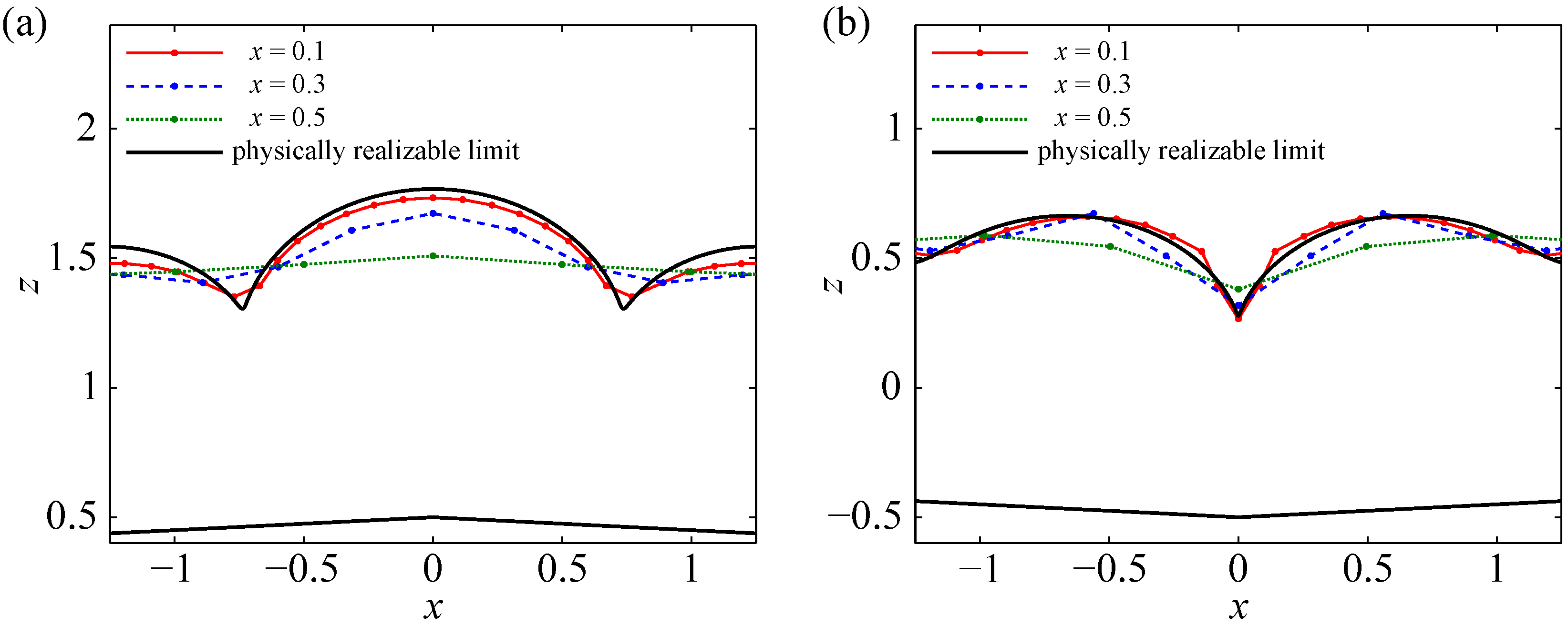
with a discontinuous first derivative at were chosen as surface profiles of 2D anodes that have a sharp “corner”. The shapes of cathodes corresponding to anodes with and were computed by applying the continuous adjoint-based shape optimization method; the mesh cell size in x direction, , was varied from to .
Figure 8 shows numerically computed cathode shapes in the vicinity of a sharp corner of a convex (Panel (a)) or concave (Panel (b)) anode.
To evaluate the plausibility of the numerical results, the limit of physically meaningful cathode shapes, which will be referred to as the “analytical limit solution”, was computed by the Fourier approximation method of the previous section.
Details of the interelectrode gap region near are shown in Figure 8. All in all, the numerically computed cathode shape approaches the “analytical limit solution” when the mesh becomes finer. The “analytical limit solution” has two singularities at when the anode is convex (Panel (a)) and one singularity at when the anode is concave (Panel (b)). At the same positions, the numerically computed cathode surface profiles also have “peaks”, which become increasingly sharp when decreases. For (not shown), the computation diverges since the cathode boundary starts forming loops at the locations of the “peaks”, similar to the situation shown in Figure 6.
The behavior of the results shown in Figure 8 bears some similarity to the behavior of the results obtained through the Fourier approximation method: with an increasing degree of the Fourier polynomial, the accuracy of the approximation of the anode improves, but the shape of the obtained cathode becomes less smooth and eventually physically meaningless (cf. Figure 7). In fact, both refining the mesh and increasing the degree of the Fourier polynomial involves an increase in the degree of freedom.
The formation of “peaks” when using a fine mesh was also mentioned by Das and Mitra [49] in a related inverse problem associated with steady-state heat conduction. However, the authors consider this phenomenon to be “unrealistic” and see its cause as due to the motion of the mesh in the numerical iteration process. As revealed by the comparison with the results obtained through the Fourier approximation method (see Figure 8), the formation of the “peaks” is not a numerical artifact but a consequence of the nature of the cathode shape design problem.
3.3. Existence of Exact and Physically Realizable Solutions
In view of the previous examples, it is important to answer the question about conditions for the theoretical existence of cathode shapes required to produce an anode of arbitrary smoothness, at least for the 2D case.
When the function F that describes the shape of the desired anode is not analytic, the complex variable method can be applied to a Fourier polynomial (Equation (22)) approximating F, as shown in the previous section. The exact shape of F is obtained in the limit of for . If F has a piecewise continuous m-th derivative, , on , and are continuous on , the Fourier coefficients satisfy . The parametric representations of the cathode, then, comprises harmonic contributions with amplitudes proportional to
which become infinite when for any integer number m. Hence, for anode surface profiles that are not representable by analytic functions, exact solutions to the cathode shape design problem do not exist.
3.4. Ill-Posedness of the Cathode Shape Design Problem and Its Consequences
In practice, workpiece geometries are often provided as interpolations by splines or freeform surfaces used in CAD models. These anode shapes are not analytic, thus violating the condition for the existence of an exact solution, as discussed in the previous section.
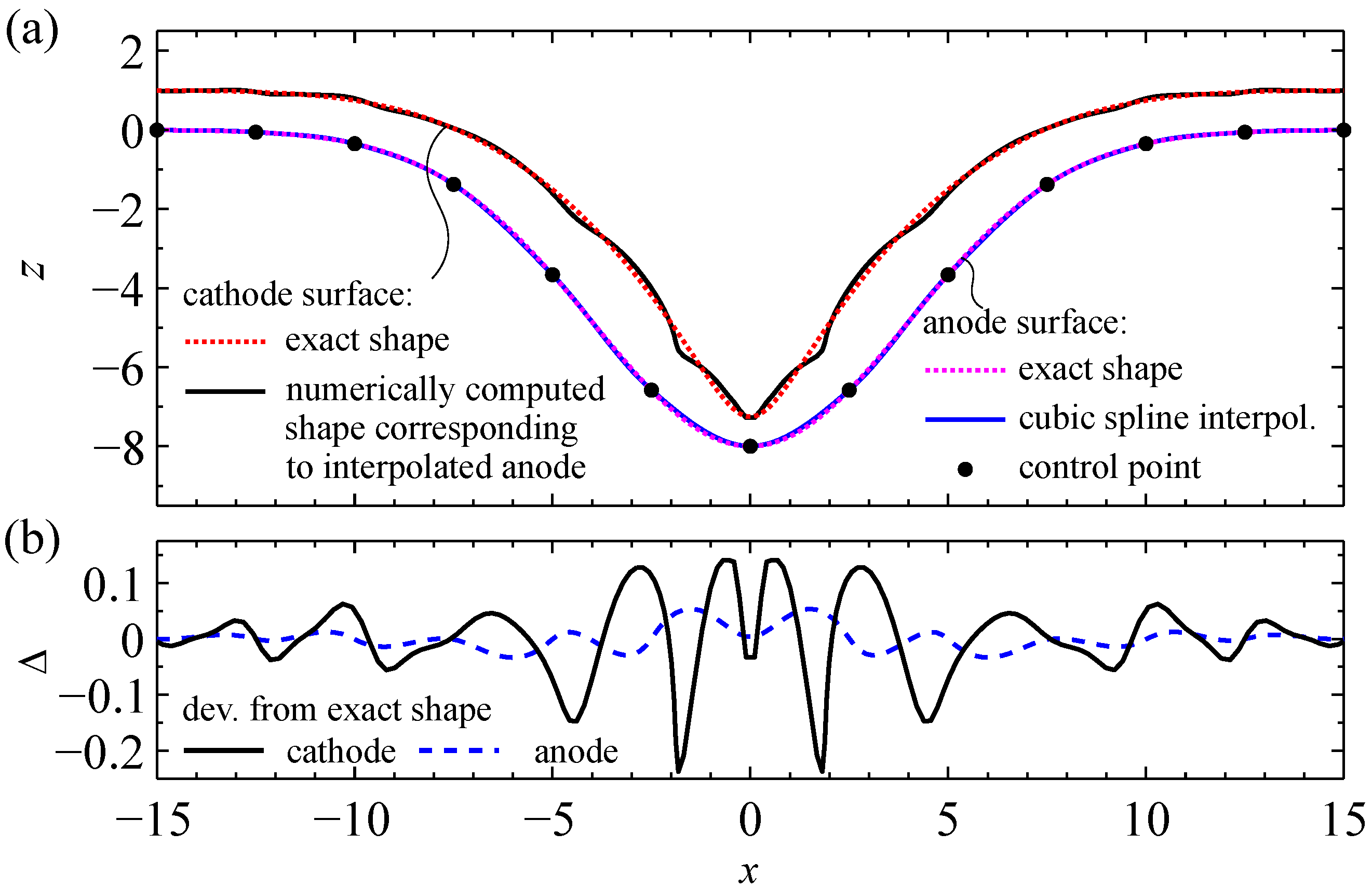
In the following, we investigated the shape of the numerically computed cathode in cases where the nominally analytic shape of a desired anode is disturbed by a nonanalytic perturbation. As an example, the 2D Gaussian-shaped anode shown in Figure 3a was chosen as the nominal anode. The “perturbed” shape of the anode was generated by interpolating the nominal anode by a cubic spline through 13 control points as illustrated in Figure 9a.
The shape of the cathode corresponding to the “perturbed”, i.e., interpolated anode shape, was obtained by adjoint-based shape optimization and will be called a “perturbed cathode shape” in the following. The surface profiles of both electrodes are shown in Figure 9a. As illustrated by the upper solid line, the numerically computed cathode surface profile exhibits features with a high curvature, which are referred to as “peaks” in the following discussion.
The deviations of the perturbed shapes of both electrodes from the respective nominal shapes (Equations (17)–(19)), which are measured in the direction of the surface normal, are shown in Figure 9b. While the maximum deviation of the nominal and the perturbed anode shape from each other is less than 6% of the gap width, the maximum deviation of the nominal and the perturbed cathode shape from each other is more than 23%. The latter deviation exceeds 25%, when the number of mesh cells along the gap is increased to . For , the simulation fails before convergence, which is caused by mesh degeneration around the “peak” of the perturbed cathode shape at , similar to the failure shown in Figure 6a.
The high sensitivity of the numerically computed cathode shape to nonanalytic perturbations of an analytic anode shape can be attributed to the ill-posed nature of the cathode shape design problem as a Cauchy problem of the Laplace equation, as mentioned by Das and Mitra [40]. As also observed, mesh refinement “deteriorates” the quality of the results in the sense that the deviation of the perturbed cathode shape from the nominal cathode shape is increased. This paradoxical behavior is often encountered when solving a discretized ill-posed problem (see [50], Section 4.1).
3.5. Perimeter Regularization for Cathode Shape Design
Stable approximate solutions to ill-posed problems can be constructed using regularization methods. In the context of the cathode shape design problem in ECM, the solution would be stable if small (nonanalytic) perturbations of the anode data, which are caused by, e.g., spline interpolation of an analytic shape, still resulted in smooth cathode shapes, which is not the case in the example shown in the previous section.
Smooth cathode shapes, in spite of nonanalytic perturbations, could be obtained by choosing a coarse mesh (cf. Figure 8), which is indeed a regularization method known as projection method [51]. However, the disadvantage of using a coarse mesh is the limited accuracy of the numerically computed physical fields.
To decouple the stability of the solution from the size of the mesh used in computations, the cathode shape design procedure by continuous adjoint-based shape optimization was extended by including the technique of perimeter regularization, which was used to stabilize ill-posed geometric inverse problems and shape optimization problems [52,53]. In the cathode shape design problem, the objective function (Equation (6)) was extended by an additional integral term that penalizes the total surface area of the unknown cathode, , i.e.,
where is the regularization parameter. To derive the reduced gradient of Equation (32), Theorem 4 in Murat and Simon [54] for the shape derivative of surface objectives applies, resulting in (cf. Equation (11))
where H is the sum of principal curvatures. The optimal shape variation direction field is then given by (cf. Equation (12) for the unregularized case)
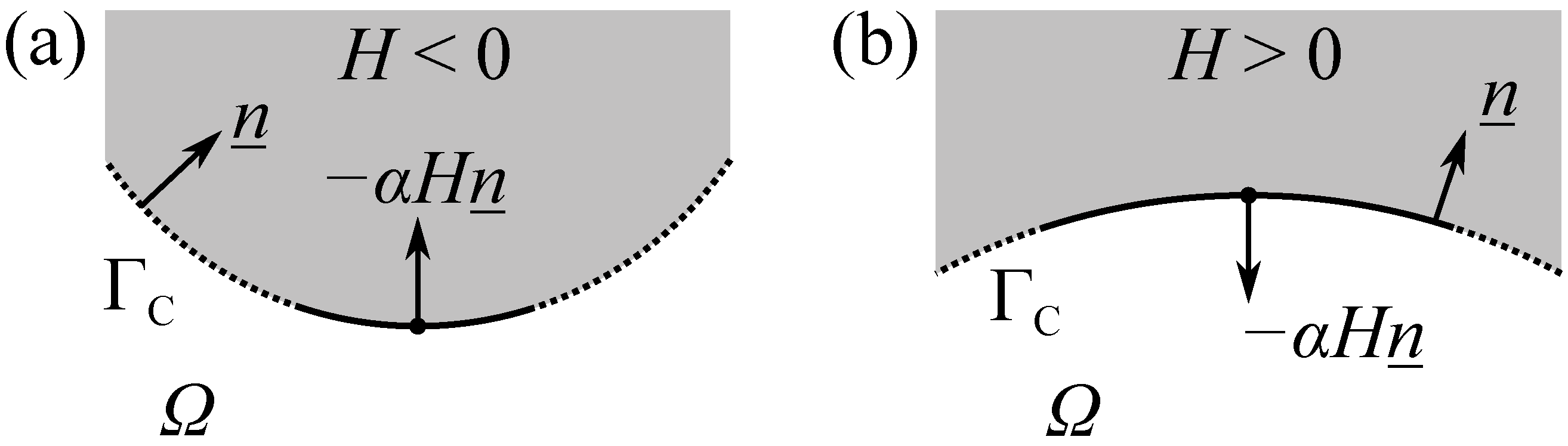
The second integral term in the objective function (32) can be interpreted as the surface energy of that tends to a minimum. Figure 10 illustrates the contribution of the term to the optimal shape variation direction field (34), where is the outer unit surface normal of the gap domain (and points into the cathode). For boundary regions in which the electrode is locally convex and the gap domain is locally concave (see Figure 10a), H is negative; hence, the vector points towards the exterior of . For boundary regions in which the cathode is locally concave and the gap domain is locally convex (see Figure 10b), the vector points towards the interior of . In both cases, the regularization term smooths the boundary .
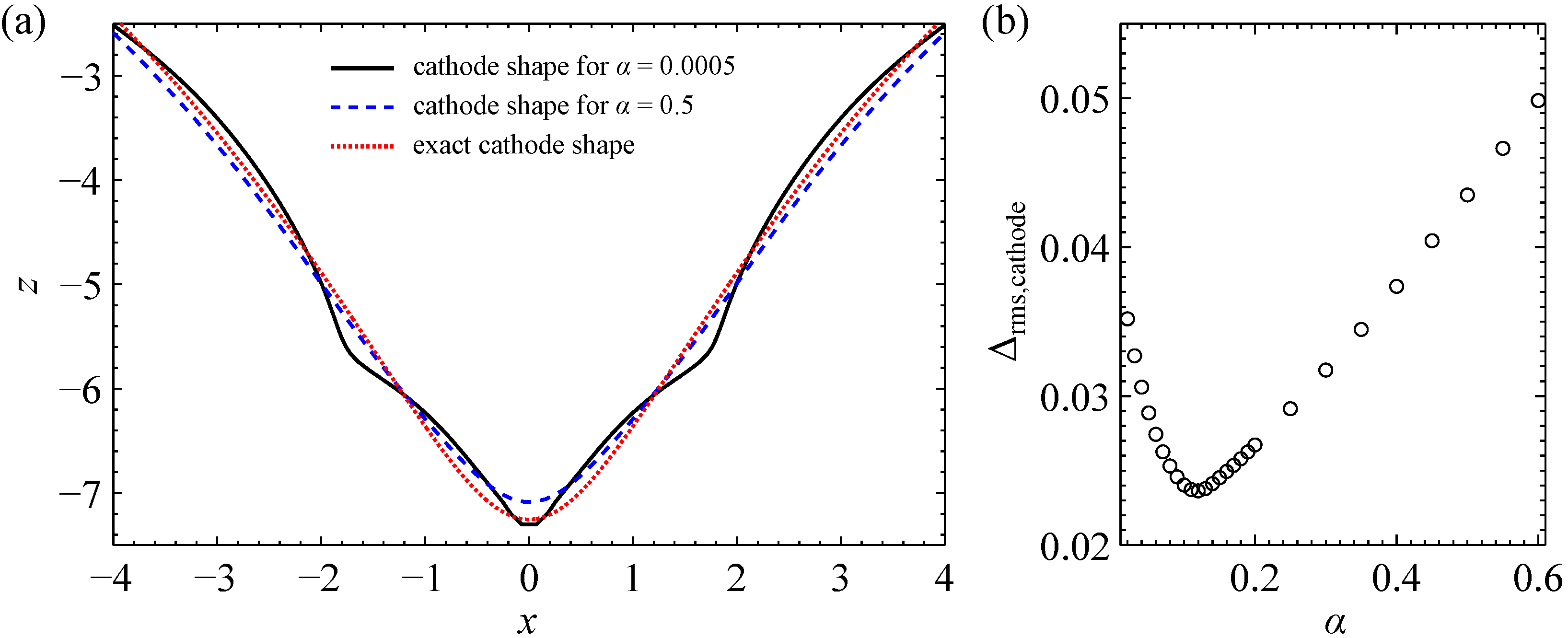
The example shown in Figure 9a was recalculated using the perimeter regularization technique with ranging from to . To illustrate the effect of regularization, the region around of two numerically computed cathode shapes is shown in Figure 11a and compared with the exact shape of the cathode. Whereas, for , the cathode surface exhibits “peaks” similar to the unregularized solution (cf. Figure 9a), the vertex at of the cathode obtained for is truncated compared with the analytical solution.
To quantify the overall difference between the analytical and numerical solutions, the mean normal deviation
of the numerically computed cathode (required to produce the spline-interpolated anode) from the exact cathode (required to produce the anode defined by the analytic function) is plotted in Figure 11b as a function of the regularization parameter, . With an increasing , first decreases, then reaches a minimum at an optimum regularization parameter of and increases for .
The function behaves in a way that is commonly observed in the regularization of ill-posed problems: for , the “error” () increases since the instability of the ill-posed inverse problem dominates; for large , the approximation of the original objective function (6) by the regularized objective function (32) becomes less accurate and is dominated by the approximation error.
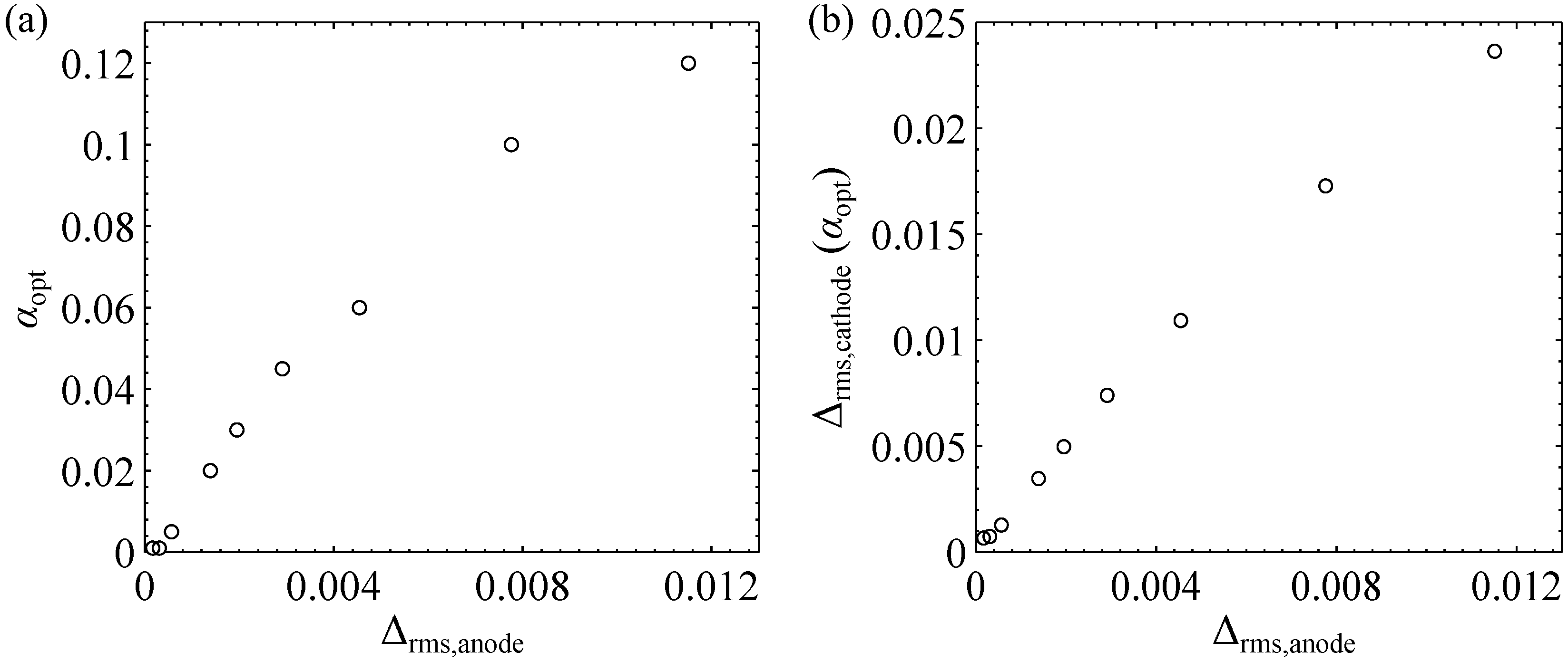
In a further study, the number of the control points for the spline interpolation of the anode shape is varied. A higher number of equidistantly distributed control points corresponds to a decrease in the mean normal deviation
of the anode, or a reduction in the “perturbation” of the given anode data. As shown in Figure 12a, the value of approaches zero when . Likewise, the quantity approaches zero when (Figure 12b). Both results indicate the admissibility of the perimeter regularization method (cf. [55] Definition 2.3).
3.6. Anode Shapes Produced by Regularized Cathodes
Perimeter regularization is shown to be an admissible regularization technique and enables the computation of stable approximate solutions to the cathode shape design problem in the case where the desired shape of the anode is not given by an analytic function. However, every regularization technique modifies the original problem to a certain extent. Hence, the cathode computed using regularization, which will be abbreviated by “regularized cathode” in the following, usually produces an anode shape (in an ECM process) that deviates from the shape of the desired anode. In practical applications, this deviation should be quantified to assess whether the regularized cathode can be used in ECM to produce the desired anode shape within predefined tolerance levels.
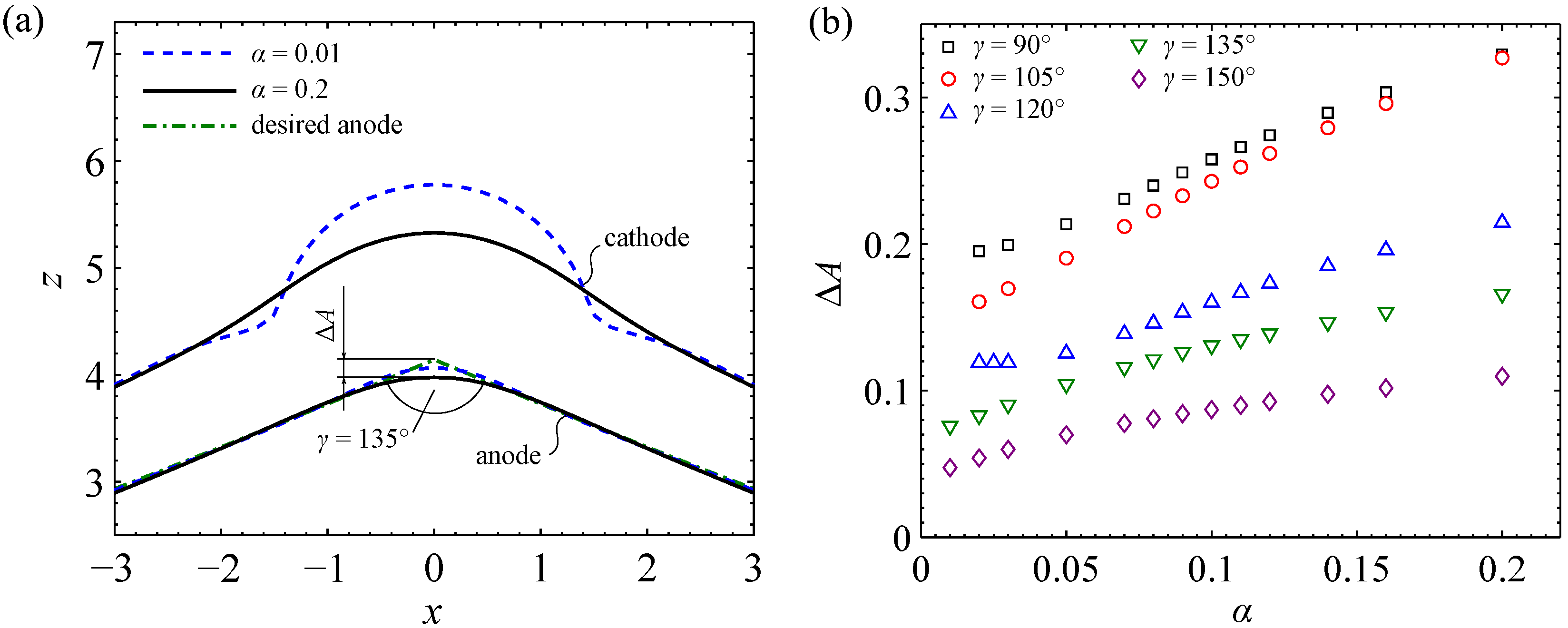
The following example illustrates the influence of the regularization parameter chosen for the cathode shape design procedure on the anode shape produced by the regularized cathode. The focus is on the rounding of originally sharp corners on the anode surface. The shapes of the desired anodes are similar to the study presented in Figure 7. Figure 13 exemplarily illustrates the results of the cathode shape design problem with for and . In the region , which is far from the tip of the corner, the cathode shapes obtained for both values of agree with each other. Large differences are observed in the vicinity of the tip of the corner: the widths of the front gaps at differ from each other by , which is half of the width of the standard equilibrium front gap. Furthermore, the cathode shape obtained for has two “peaks” at , which are not observed in the case of .
The steady-state shapes of anodes obtained in an ECM process using the regularized cathodes were computed to verify the quality of the designed cathodes. As illustrated in Figure 13a, the anode shapes produced by regularized cathodes have a rounded corner, where the radius of the rounding is larger for than for . The largest deviation of the resulting obtained shapes from the desired shapes of the anode is found at , which is quantified by , as indicated in the inset of Figure 13a.
Regularized cathode shapes were computed for a series of anodes with values of the opening angle between and and values of the regularization parameter ranging from to (in the cases with , the simulation is unstable for ). The quantity was determined for all anodes produced by the computed regularized cathode shapes.
As illustrated in Figure 13b, increases with increasing values of , indicating that the least regularized cathode (with sharp “peaks” on its surface) that can be computed stably would produce the anode with the most precise shape. This phenomenon is also observed in Figure 7, where the precision of the shape of the produced anode increases whereas the shape of the cathode “deteriorates” due to the formation of singularities and loops (cf. Figure 7). Furthermore, the value of obtained for a given regularization parameter decreases with an increasing value of the angle .
In practice, however, since the regularized cathode shape obtained for low values of the regularization parameter is usually less smooth, which could adversely affect the flow of the electrolyte, choosing a higher value of could be advantageous as long as the shape of the anode produced by the regularized cathode fulfills the tolerance requirements.
4. Conclusions
The analytical and numerical studies presented in the previous section answer the three questions posed in the introduction:
- When the function F describing the surface profile of the anode is analytic, the theoretical shape of the cathode can be calculated analytically using the complex variable method. However, the physical realizability of the cathode depends on the aspect ratio of features on the anode surface and the width of the standard equilibrium front gap. When F is not analytic, especially when F is represented by piecewise interpolation as in most engineering cases, exact solutions of the cathode shape problem do not exist at all.
- When an exact and physically realizable cathode shape exists, the continuous adjoint-based shape optimization method is shown to be able to compute cathode shapes with an accuracy of 2 ‰ of the interelectrode gap using a sufficiently fine mesh. The accuracy increases with an increasing mesh refinement. When an exact and physically realizable cathode shape does not exist, singularities such as kinks and loops form on the cathode boundary in the course of the iterative optimization process. The formation of singularities becomes more severe with an increasing mesh refinement. This phenomenon is not a numerical artifact but is due to the nature of the ill-posed inverse problem.
- Smooth and physically realizable approximate solutions for the cathode shape can be obtained through perimeter regularization. The smoothness of the approximated cathode is controlled by the regularization parameter, where the latter should be chosen in such a way that the shape of the anode produced by the approximate cathode is within the range of manufacturing tolerance.
Author Contributions
Conceptualization, J.L. and E.A.W.; methodology, J.L.; software, J.L.; validation, J.L.; formal analysis, J.L.; investigation, J.L.; resources, E.A.W.; writing—original draft preparation, J.L. and E.A.W.; writing—review and editing, J.L. and E.A.W.; visualization, J.L.; supervision, E.A.W.; project administration, E.A.W. All authors have read and agreed to the published version of the manuscript.
Funding
This research received no external funding.
Data Availability Statement
Due to the non-disclosure agreement signed with the industrial partner, experimental data are not allowed to be published.
Conflicts of Interest
The authors declare no conflict of interest.
Abbreviations
| 2D, 3D | Two-, three-dimensional |
| ECM | Electrochemical machining |
| OpenFOAM® | “Open-source Field Operation And Manipulation” (C++ toolbox for the |
| development of customized numerical solvers) | |
| Symbols, over- and undersets | |
| (tilde) | Dimensioned physical quantity |
| (underline) | Vector quantity or operator |
| Nabla operator | |
| Normal derivative on a boundary | |
| Partial shape derivative of J at in the direction | |
| of the deformation velocity field | |
| Total derivative with respect to x | |
| Total shape derivative of the reduced objective function j at | |
| in direction of the deformation velocity field | |
| Upper-case Roman | |
| A | Amplitude parameter characterizing the vertical extension of |
| the anode profile | |
| Critical value of A relevant to the physical realizability of solutions | |
| Function describing the anode profile | |
| Fourier polynomial of degree N approximating | |
| Maximum of the shape gradient | |
| H | Sum of principal curvatures |
| J, | (Regularized) objective function |
| L | Width parameter characterizing the horizontal extension of the anode profile |
| N | Degree of the Fourier polynomial |
| Number of mesh cells along the gap | |
| Maximum degree of the Fourier polynomial for physically | |
| realizable solutions to exist | |
| Lower-case Roman | |
| , | Coefficients of the Fourier polynomial approximating the anode profile |
| , | Coefficients of the Fourier polynomial approximating the cathode profile |
| , | (Dimensionless) standard front gap width |
| Initial standard front gap width | |
| Standard equilibrium front gap width | |
| j, | (Regularized) reduced objective function |
| n | Index |
| Outer unit normal of anode boundary | |
| Deformation velocity field (continuous) | |
| Component of deformation velocity field in boundary | |
| normal direction | |
| Dimensionless anode dissolution velocity | |
| Dimensionless cathode feed velocity | |
| x, y, z | Dimensionless spacial coordinates |
| ,, | Coordinates of points on cathode and anode boundaries |
| Upper-case Greek | |
| Boundary (in general) | |
| Dimensionless anode boundary | |
| Dimensionless cathode boundary | |
| Dimensionless non-metallic side boundary | |
| Normal deviation of the computed electrode profile from the exact profile | |
| Deviation of the amplitude of the computed electrode profile | |
| from the exact amplitude | |
| Mean normal deviation of computed electrode profile | |
| Mesh size along the gap direction | |
| Dimensionless electric potential | |
| Dimensionless calculation domain | |
| Total boundary of the dimensionless calculation domain | |
| Deformed calculation domain | |
| Lower-case Greek | |
| (Optimum) regularization parameter | |
| Opening angle (see Figure 13) | |
| Maximum of the integrand of the shape optimization | |
| objective function | |
| Angle between feed direction and anode surface normal | |
| Lagrange multipliers for calculation domain, anode, cathode, and | |
| non-metallic side boundary | |
| Standard deviation of the Gaussian | |
| Iteration step length | |
| Curve parameter | |
Appendix A. Experimental Tests of the Potential Model
Appendix A.1. Outline
In parallel to the theoretical and numerical studies, several experiments were conducted to test if the potential model (see Section 2.1) can describe an ECM experiment under near-ideal conditions. Since the materials and the experimental setup were also used by an industrial partner for commercial applications, technical details and absolute values of the process parameters are omitted throughout this chapter due to obligations resulting from a non-disclosure agreement.
Appendix A.2. Materials and Experimental Setup
Samples made of a nickel-based alloy were processed on a single-axis laboratory ECM set-up. Aqueous solution of sodium nitrate was used as electrolyte, whose temperature and pH value were controlled to maintain the electrolyte conductivity as constant as possible.
The gap width was measured by touching, i.e., by turning off the machining voltage and recording the distance so that the tool can be further advanced until mechanical contact with the workpiece is established. The process current was measured inductively and monitored during machining. The voltage across the interelectrode gap was measured as potential difference between tool and workpiece. The widths of the interelectrode gaps were in the magnitude of several hundreds micrometers, ensuring the effective removal of reaction products in the interelectrode gap.
Appendix A.3. Transition into Steady State
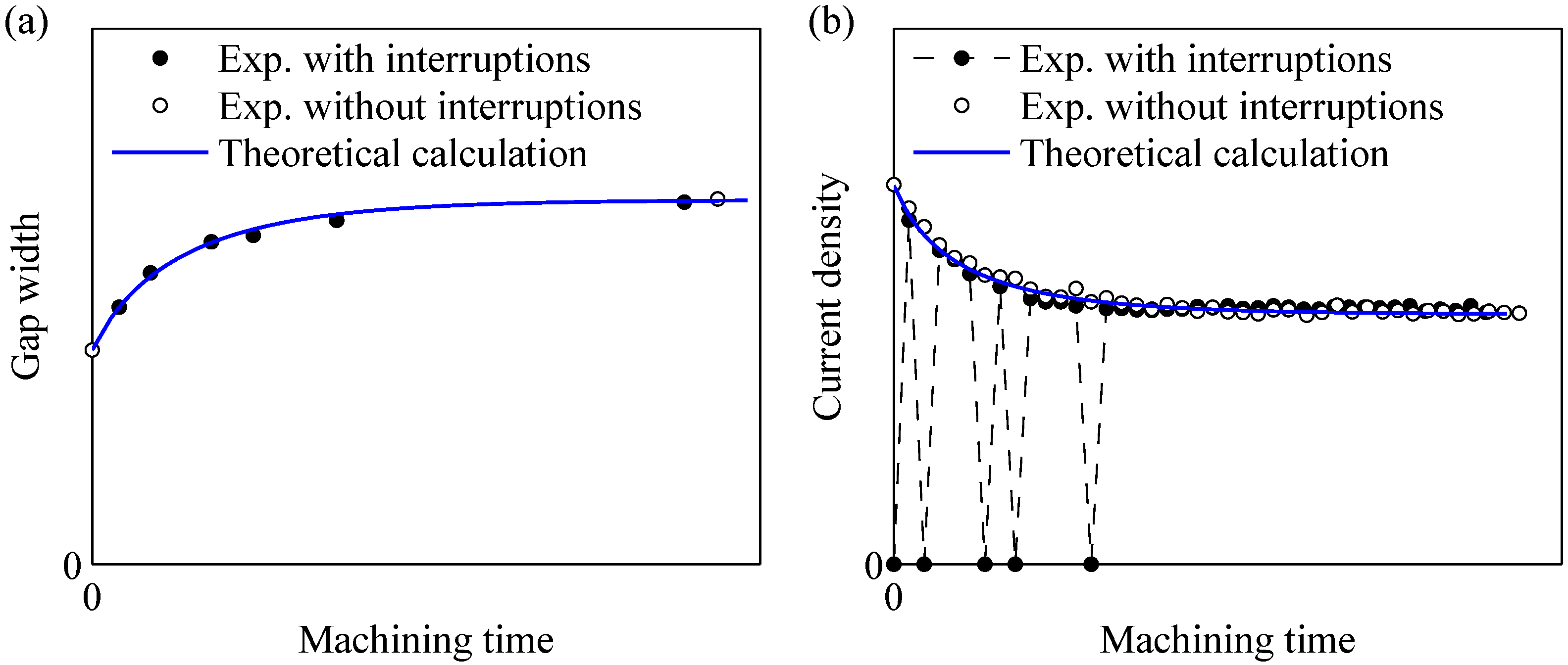
Since the formulation of the inverse problem is based on the shape of the anode in steady state (see Section 2.2), ECM experiments were carried out to investigate if the potential model can describe the steady state, including the instationary transition at the beginning of an ECM process. The machining parameters were chosen such that the initial gap widths () deviated from the standard equilibrium front gap widths () by more than 30%. The process was interrupted after certain time intervals to determine the gap widths during the transition stage. A continuous experiment under the same machining conditions, but without interruptions, was carried out to check the influence of the interruptions on the process.
The panels (a) and (b) in Figure A1 show, as an example, the evolution of the gap width and the current density, respectively. The solid lines in both panels represent the theoretical evolution of the corresponding quantities. Both the experimental and the theoretical gap widths increase with time and asymptotically approach an upper limit. The experimental gap widths deviate from the theoretical values by less than 3%. Apart from five zero values in the experiment with interruptions, the experimental as well as the theoretical current density decrease with time and asymptotically approach a lower limit. The maximum deviation between the experimental and the theoretical current density is less than 5%.
The zero values of the current density evolution in Figure A1b are attributed to the interruption of the process for gap width determination. However, the nonzero current density values of the experiment with interruptions agree with those obtained in the continuous experiment within experimental uncertainties, indicating that the interruptions do not significantly disturb the overall process. The experimental data agree with the theoretical calculation for both the gap width and the current density evolution; hence, under the process conditions of this example, the potential model can be used to describe the current density and the gap width during the transition stage of a basic ECM experiment.
Figure A1.
Evolution of the gap width (panel (a)) and the current density (panel (b)) in an ECM experiment at constant feed rate compared with theoretical computations based on the potential model. (The scales are omitted due to reasons of non-disclosure).
Figure A1.
Evolution of the gap width (panel (a)) and the current density (panel (b)) in an ECM experiment at constant feed rate compared with theoretical computations based on the potential model. (The scales are omitted due to reasons of non-disclosure).

Appendix A.4. Anode Shapes in Steady State
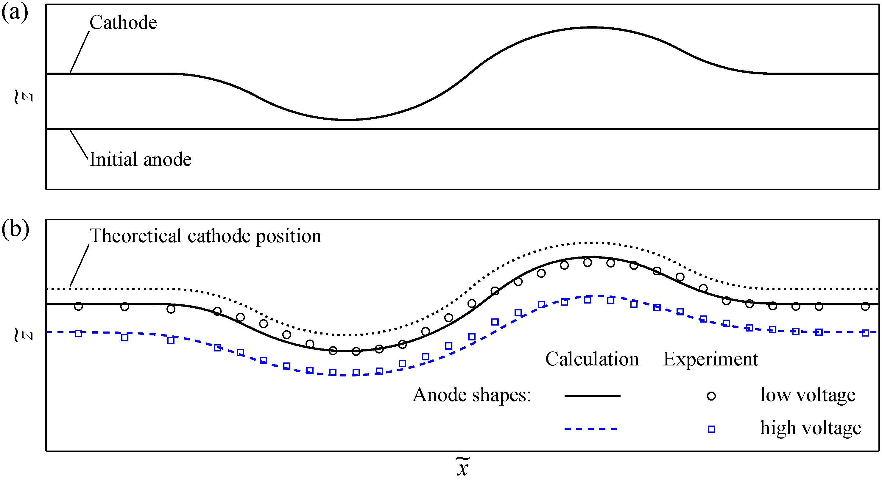
ECM using curved tools was studied using a quasi 2D cathode consisting of two plane regions at the borders and a sine-like shape composed of arcs in the center (see Figure A2a). The experiments were carried out at two different values of the machining voltage while the feed rate was kept fixed. The initially plane anode was machined electrochemically until the process reached the steady-state indicated by a constant process current. The anode shape after machining was determined by scanning the machined surface using a digital indicator. The “theoretical” shapes of the anodes were computed using the simulation tool, whose implementation is described in more details in Section 2.2. The initial gap geometry shown in Figure A2a was used as the initial computational domain; values of voltage and feed rate used in the experiments were used as input parameters for the simulation.
Figure A2.
ECM using curved tool electrode. Panel (a) shows the cross section of the initial configuration of tool and workpiece. Panel (b) shows workpiece surfaces after ECM two gap voltages, while the feed rate in both experiments are equal.
Figure A2.
ECM using curved tool electrode. Panel (a) shows the cross section of the initial configuration of tool and workpiece. Panel (b) shows workpiece surfaces after ECM two gap voltages, while the feed rate in both experiments are equal.

Figure A2b displays experimental and simulated anode shapes obtained for two values of gap voltages. The position of the cathode obtained in the simulation is indicated as well to visualize the shape of the steady-state interelectrode gap. As evident from Figure A2b, the results of the experiments agree quite well with those obtained in the simulations. They show that the underlying potential model is sufficient for describing the (continuous-mode) ECM process in our cases, where the widths of the interelectrode gaps are in the magnitude of several hundreds micrometers, ensuring the effective removal of reaction products in the interelectrode gap. However, more complex models would be needed if the interelectrode gap widths were smaller or when working with pulsed current, such as, e.g., in precise electrochemichal machining (PECM).
References
- Burger, M.; Koll, L.; Werner, E.; Platz, A. Electrochemical machining characteristics and resulting surface quality of the nickel-base single-crystalline material LEK94. J. Manuf. Process. 2012, 14, 62–70. [Google Scholar] [CrossRef]
- Xu, Z.; Wang, Y. Electrochemical machining of complex components of aero-engines: Developments, trends, and technological advances. Chin. J. Aeronaut. 2021, 34, 28–53. [Google Scholar] [CrossRef]
- Ziegler, C.; Beetz, S.; Scherer, R.; Moser, S. Tool for the Electrochemical Machining of a Fuel Injection Device. European Patent EP 1 893 379 B1, 28 March 2012. [Google Scholar]
- Harlow, R.A.; Kimball, R.C. Electrochemical Machining of Automatic Gun Barrels. Technical Report AFATL-TR-74-87. United States Air Force Armament Laboratory. 1974. Available online: http://www.dtic.mil/dtic/tr/fulltext/u2/b002472.pdf (accessed on 31 August 2014).
- Zinger, O.; Zhao, G.; Schwartz, Z.; Simpson, J.; Wieland, M.; Landolt, D.; Boyan, B. Differential regulation of osteoblasts by substrate microstructural features. Biomaterials 2005, 26, 1837–1847. [Google Scholar] [CrossRef]
- Schuster, R.; Kirchner, V.; Allongue, P.; Ertl, G. Electrochemical micromachining. Science 2000, 289, 98–101. [Google Scholar] [CrossRef] [PubMed]
- Rajurkar, K.; Sundaram, M.; Malshe, A. Review of Electrochemical and Electrodischarge Machining. Procedia CIRP 2013, 6, 13–26. [Google Scholar] [CrossRef] [Green Version]
- Lu, J.; Riedl, G.; Kiniger, B.; Werner, E.A. Three-dimensional tool design for steady-state electrochemical machining by continuous adjoint-based shape optimization. Chem. Eng. Sci. 2014, 106, 198–210. [Google Scholar] [CrossRef]
- Hinduja, S.; Kunieda, M. Modelling of ECM and EDM processes. CIRP Ann.-Manuf. Technol. 2013, 62, 775–797. [Google Scholar] [CrossRef]
- Gomez-Gallegos, A.; Mill, F.; Mount, A.R.; Duffield, S.; Sherlock, A. 3D multiphysics model for the simulation of electrochemical machining of stainless steel (SS316). Int. J. Adv. Manuf. Technol. 2018, 95, 2959–2972. [Google Scholar] [CrossRef] [Green Version]
- Hotoiu, E.L.; Deconinck, J. A novel pulse shortcut strategy for simulating nano-second pulse electrochemical micro-machining. J. Appl. Electrochem. 2014, 44, 1225–1238. [Google Scholar] [CrossRef]
- Liu, W.; Ao, S.; Luo, Z. Multi-physics Simulation of the Surface Polishing Effect During Electrochemical Machining. Int. J. Electrochem. Sci. 2019, 14, 7773–7789. [Google Scholar] [CrossRef]
- Klocke, F.; Heidemanns, L.; Zeis, M.; Klink, A. A Novel Modeling Approach for the Simulation of Precise Electrochemical Machining (PECM) with Pulsed Current and Oscillating Cathode. Procedia CIRP 2018, 68, 499–504. [Google Scholar] [CrossRef]
- Wu, M.; Arshad, M.H.; Saxena, K.K.; Qian, J.; Reynaerts, D. Profile prediction in ECM using machine learning. Procedia CIRP 2022, 113, 410–416. [Google Scholar] [CrossRef]
- Khalaj, G.; Azimzadegan, T.; Khoeini, M.; Etaat, M. Artificial neural networks application to predict the ultimate tensile strength of X70 pipeline steels. Neural Comput. Appl. 2013, 23, 2301–2308. [Google Scholar] [CrossRef]
- Khalaj, G.; Pouraliakbar, H.; Mamaghani, K.R.; Khalaj, M.J. Modeling the correlation between heat treatment, chemical composition and bainite fraction of pipeline steels by means of artificial neural networks. Neural Netw. World 2013, 23, 351–367. [Google Scholar] [CrossRef] [Green Version]
- Khalaj, G.; Nazari, A.; Pouraliakbar, H. Prediction of martensite fraction of microalloyed steel by artificial neural networks. Neural Netw. World 2013, 23, 117–130. [Google Scholar] [CrossRef] [Green Version]
- Tipton, H. Calculation of tool shape for ECM. In Fundamentals of Electrochemical Machining; Faust, C.L., Ed.; Electrochemical Society Softbound Symposium Series; The Electrochemical Society: Princeton, NJ, USA, 1971; pp. 87–102. [Google Scholar]
- Jain, V.; Pandey, P. Tooling design for ECM. Precis. Eng. 1980, 2, 195–206. [Google Scholar] [CrossRef]
- Krylov, A.L. The Cauchy problem for the Laplace equation in the theory of electrochemical metal machining. Sov. Phys.-Dokl. 1968, 13, 15–17. [Google Scholar]
- Nilson, R.; Tsuei, Y. Inverted Cauchy problem for the Laplace equation in engineering design. J. Eng. Math. 1974, 8, 329–337. [Google Scholar] [CrossRef]
- Alder, G.; Clifton, D.; Mill, F. A direct analytical solution to the tool design problem in electrochemical machining under steady state conditions. Proc. Inst. Mech. Eng. Part B J. Eng. Manuf. 2000, 214, 745–750. [Google Scholar] [CrossRef]
- McClennan, J.; Alder, G.; Sherlock, A.; Mill, F.; Clifton, D. Two-dimensional tool design for two-dimensional equilibrium electrochemical machining die-sinking using a numerical method. Proc. Inst. Mech. Eng. Part B J. Eng. Manuf. 2006, 220, 637–645. [Google Scholar] [CrossRef]
- Zhu, D.; Wang, K.; Yang, J. Design of Electrode Profile In Electrochemical Manufacturing Process. CIRP Ann.-Manuf. Technol. 2003, 52, 169–172. [Google Scholar] [CrossRef]
- Sun, C.; Zhu, D.; Li, Z.; Wang, L. Application of FEM to tool design for electrochemical machining freeform surface. Finite Elem. Anal. Des. 2006, 43, 168–172. [Google Scholar] [CrossRef]
- Demirtas, H.; Yilmaz, O.; Kanber, B. A simplified mathematical model development for the design of free-form cathode surface in electrochemical machining. Mach. Sci. Technol. 2017, 21, 157–173. [Google Scholar] [CrossRef]
- Reddy, M.S.; Jain, V.K.; Lal, G.K. Tool Design for ECM: Correction Factor Method. J. Eng. Ind. 1988, 110, 111–118. [Google Scholar] [CrossRef]
- Jain, V.K. An Analysis of ECM Process for Anode Shape Prediction. Ph.D. Thesis, University of Roorkee, Roorkee, India, 1980. [Google Scholar]
- Jain, V.K.; Pandey, P.C. Tooling design for ECM—A finite element approach. J. Eng. Ind. 1981, 103, 183–191. [Google Scholar] [CrossRef]
- Jain, V.K.; Pandey, P.C. Investigations into the use of bits as a cathode in ECM. Int. J. Mach. Tool Des. Res. 1982, 22, 341–352. [Google Scholar] [CrossRef]
- Jain, V.K.; Rajurkar, K.P. An integrated approach for tool design in ECM. Precis. Eng. 1991, 13, 111–124. [Google Scholar] [CrossRef]
- Narayanan, O.H.; Hinduja, S.; Nobel, C.F. Design of Tools for Electrochemical Machining by the Boundary Element Method. Proc. Inst. Mech. Eng. Part C J. Mech. Eng. Sci. 1986, 200, 195–205. [Google Scholar] [CrossRef]
- Hardisty, H.; Mileham, A.R. Finite element computer investigation of the electrochemical machining process for a parabolically shaped moving tool eroding an arbitrarily shaped workpiece. Proc. Inst. Mech. Eng. Part B J. Eng. Manuf. 1999, 213, 787–798. [Google Scholar] [CrossRef]
- Bhattacharyya, S.; Ghosh, A.; Mallik, A. Cathode shape prediction in electrochemical machining using a simulated cut-and-try procedure. J. Mater. Process. Technol. 1997, 66, 146–152. [Google Scholar] [CrossRef]
- Zhu, D.; Liu, C.; Xu, Z.; Liu, J. Cathode design investigation based on iterative correction of predicted profile errors in electrochemical machining of compressor blades. Chin. J. Aeronaut. 2016, 29, 1111–1118. [Google Scholar] [CrossRef]
- Fang, M.; Chen, Y.; Jiang, L.; Su, Y.; Liang, Y. Optimal design of cathode based on iterative solution of multi-physical model in pulse electrochemical machining (PECM). Int. J. Adv. Manuf. Technol. 2019, 105, 3261–3270. [Google Scholar] [CrossRef]
- Gu, Z.; Zhu, W.; Zheng, X.; Bai, X. Cathode tool design and experimental study on electrochemical trepanning of blades. Int. J. Adv. Manuf. Technol. 2019, 100, 857–863. [Google Scholar] [CrossRef]
- Hunt, R. An Embedding Method For the Numerical-solution of the Cathode Design Problem In Electrochemical Machining. Int. J. Numer. Methods Eng. 1990, 29, 1177–1192. [Google Scholar] [CrossRef]
- Chang, C.; Hourng, L. Two-dimensional two-phase numerical model for tool design in electrochemical machining. J. Appl. Electrochem. 2001, 31, 145–154. [Google Scholar] [CrossRef]
- Das, S.; Mitra, A.K. Use of boundary element method for the determination of tool shape in electrochemical machining. Int. J. Numer. Methods Eng. 1992, 35, 1045–1054. [Google Scholar] [CrossRef]
- Zhou, Y.; Derby, J.J. The cathode design problem in electrochemical machining. Chem. Eng. Sci. 1995, 50, 2679–2689. [Google Scholar] [CrossRef]
- Hadamard, J. Lectures on Cauchy’s Problem in Linear Partial Differential Equations; Mrs. Hepsa Ely Silliman Memorial Lectures; Yale University Press: New Haven, CY, USA, 1923. [Google Scholar]
- McGeough, J.A.; Rasmussen, H. On the derivation of the quasi-steady model in electrochemical machining. IMA J. Appl. Math. 1974, 13, 13–21. [Google Scholar] [CrossRef]
- Deconinck, J. Current Distributions and Electrode Shape Changes in Electrochemical Systems; Springer: Berlin, Germany, 1992. [Google Scholar]
- Klocke, F.; König, W. Fertigungsverfahren 3: Abtragen, Generieren, Lasermaterialbearbeitung, 4th ed.; Springer: Berlin, Germany, 2006. [Google Scholar]
- Gileadi, E. Physical Electrochemistry; Wiley: Weinheim, Germany, 2011. [Google Scholar]
- Patankar, S. Numerical Heat Transfer and Fluid Flow; McGRAW-HILL: New York, NY, USA, 1980. [Google Scholar]
- Löhner, R.; Yang, C. Improved ALE mesh velocities for moving bodies. Commun. Numer. Methods Eng. 1996, 12, 599–608. [Google Scholar] [CrossRef]
- Das, S.; Mitra, A.K. An algorithm for the solution of inverse laplace problems and its application in flaw identification in materials. J. Comput. Phys. 1992, 99, 99–105. [Google Scholar] [CrossRef]
- Colton, D.; Kress, R. Inverse Acoustic and Electromagnetic Scattering Theory, 3rd ed.; Applied Mathematical Sciences; Springer: New York, NY, USA, 2013. [Google Scholar]
- Natterer, F. Regularisierung schlecht gestellter Probleme durch Projektionsverfahren. Numer. Math. 1977, 28, 329–341. [Google Scholar] [CrossRef]
- Burger, M.; Osher, S.J. A survey on level set methods for inverse problems and optimal design. Eur. J. Appl. Math. 2005, 16, 263–301. [Google Scholar] [CrossRef] [Green Version]
- Hackl, B. Methods for Reliable Topology Changes for Perimeter-Regularized Geometric Inverse Problems. SIAM J. Numer. Anal. 2007, 45, 2201–2227. [Google Scholar] [CrossRef] [Green Version]
- Murat, F.; Simon, J. Etude de problemes d’optimal design. In Optimization Techniques Modeling and Optimization in the Service of Man Part 2; Cea, J., Ed.; Lecture Notes in Computer Science; Springer: Berlin, Germany, 1976; Volume 41, pp. 54–62. [Google Scholar] [CrossRef]
- Kirsch, A. An Introduction to the Mathematical Theory of Inverse Problems; Applied Mathematical Sciences; Springer: New York, NY, USA, 2011. [Google Scholar]
Figure 1.
Principle of electrochemical machining (ECM). (a) Initial configuration consisting of a cathode tool of a defined shape and a plane anode workpiece to be machined. The tool is advanced towards the workpiece at a defined feed rate. Electrical current flows when a voltage is applied across the gap; the thin red lines between the electrodes illustrate the current density. (b) Steady-state configuration of tool and workpiece. The final shape of the workpiece is approximately the negative image of the tool electrode. The inter-electrode gap is the calculation domain of the model used in this work. The boundaries and are defined by tool (cathode) and workpiece (anode) surfaces, respectively, and is the non-metallic side boundary through which the electrical current flux is zero. For each point on the workpiece boundary , is defined as the angle between the outer boundary unit normal vector and the feed direction unit vector . “Front gap” refers to an inter-electrode gap region where the workpiece surface is perpendicular to the feed direction (i.e., ). “Standard front gap” (with steady-state width ) is a front gap region where the electrodes are plane (figure adapted from Ref. [8]).

Figure 2.
Flowchart of the cathode shape design algorithm based on continuous adjoint shape optimization.
Figure 2.
Flowchart of the cathode shape design algorithm based on continuous adjoint shape optimization.

Figure 3.
Cathode shapes (solid lines) required to produce Gaussian anode shapes (dashed lines) defined by Equation (17) with (spatial dimensions are normalized to the width of the standard equilibrium front gap). The solutions in parametric form are given by Equations (18) and (19). The scale on the z-axis and the legend of Panel (a) apply for all three panels. Panel (a) shows the example with , resulting in a regular cathode shape. Panel (b) shows the anode with (see Equation (20) in the text), for which, the computed cathode is singular and represents the limit of physically realizable cathode shapes. Panel (c) shows a non-physical solution to a cathode shape obtained for a Gaussian anode with .

Figure 4.
Two-dimensional cathode shape design example. In Panel (a), the black dashed line shows the anode shape defined by Equation (17) with and ; the geometry of the cathode at the beginning of the tool design iteration is represented by the dotted black line obtained from equidistantly offsetting the anode geometry by 1; the cathode shape obtained from iterative optimization (solid line) overlaps with the analytical solution (dash-dotted line) obtained from Equations (18) and (19). Panel (b) shows the deviation of the numerical result from the analytical solution in surface normal direction.

Figure 5.
Mesh dependence of the maximum normal deviation, . The number of mesh cells along the gap is 200, and the number of cells across the gap is denoted by . The number of iterations carried out is 200 at step length .
Figure 5.
Mesh dependence of the maximum normal deviation, . The number of mesh cells along the gap is 200, and the number of cells across the gap is denoted by . The number of iterations carried out is 200 at step length .

Figure 6.
Numerical cathode shape design procedure applied to a problem without physically meaningful solution (spatial dimensions are normalized to the width of the standard equilibrium front gap). Panel (a) shows the degenerated cathode surface profile near . Panel (b) shows the evolution of the convergence measure, (cf. Equation (14)). The sudden increase after 130 iterations is attributed to the error resulting from the degenerated mesh.

Figure 7.
Example of cathode shape design for anodes with limited smoothness (spatial dimensions are normalized to the width of the standard equilibrium front gap). The 2D anode surface defined by the graph of the function defined by Equation (25) with and (thin dash-dotted line) is approximated by Fourier polynomials (Equation (26)) with , 20, and 30, which are illustrated by the solid, dashed, and dotted lines, respectively; the same line types are used to illustrate the corresponding cathodes obtained from Equations (28) and (29). The inset shows details of the exact anode and its approximations around and with R exemplarily denoting the radius of the curvature of the approximated anode () at . The quantity is the difference between the height of the approximated anode surface and that of the exact anode surface.

Figure 8.
Cathode shapes in the vicinity of a sharp corner of a convex (Panel (a), in Equation (30)) or concave (Panel (b), in Equation (30)) anode. Spatial dimensions are normalized to the width of the standard equilibrium front gap. The quantity denotes the mesh cell size in x direction used in the computation. The circles on the lines mark the positions of the mesh vertices. The upper solid line illustrates the limit of the physically realizable shape of the cathode.

Figure 9.
Cathode shape design for an anode interpolated by cubic splines (spatial dimensions are normalized to the width of the standard equilibrium front gap). The exact surface profile of the anode (dashed curve) in Panel (a) is defined by Equation (17) with and ; the surface profile of the “perturbed” anode (solid curve) is obtained by a cubic spline interpolation connecting 13 control points on the exact anode. The numerically calculated cathode to “perturbed” anode is obtained after 800 iterations at step length . The interelectrode gap is discretized by a mesh. Panel (b) shows the deviation of the “perturbed” electrode shapes from the exact shapes in surface normal direction.

Figure 10.
Smoothing effect of the regularization term on the boundary motion in a convex (Panel (a)) or concave (Panel (b)) region of the cathode.
Figure 10.
Smoothing effect of the regularization term on the boundary motion in a convex (Panel (a)) or concave (Panel (b)) region of the cathode.

Figure 11.
Influence of the regularization parameter on the computed cathode shape (spatial dimensions are normalized to the width of the standard equilibrium front gap). The prescribed anode is the cubic spline connecting 13 control points shown in Figure 9. Panel (a) shows the region around the vertex of the cathode (cf. Figure 9a). Panel (b) shows the mean normal deviation of the numerically computed cathode from the analytical solution (see Equation (35)) as a function of .

Figure 12.
Optimum regularization parameter (Panel (a)) and error in cathode shape (Panel (b)) as a function of the error in anode shape. The deviation of the prescribed anode from the ideal anode is varied by varying the number of control points in spline interpolation (cf. Figure 9a).
Figure 12.
Optimum regularization parameter (Panel (a)) and error in cathode shape (Panel (b)) as a function of the error in anode shape. The deviation of the prescribed anode from the ideal anode is varied by varying the number of control points in spline interpolation (cf. Figure 9a).

Figure 13.
Anode shapes produced by regularized cathodes (spatial dimensions are normalized to the width of the standard equilibrium front gap). (a) The prescribed anode (dash-dotted line) has an opening angle of . The panel shows details of the anode around and with exemplarily denoting the difference in the amplitude of the computed anode from the nominal value A. (b) The values of obtained from the numerical computation at different angles are illustrated by the symbols.

Disclaimer/Publisher’s Note: The statements, opinions and data contained in all publications are solely those of the individual author(s) and contributor(s) and not of MDPI and/or the editor(s). MDPI and/or the editor(s) disclaim responsibility for any injury to people or property resulting from any ideas, methods, instructions or products referred to in the content. |
© 2023 by the authors. Licensee MDPI, Basel, Switzerland. This article is an open access article distributed under the terms and conditions of the Creative Commons Attribution (CC BY) license (https://creativecommons.org/licenses/by/4.0/).
Share and Cite
MDPI and ACS Style
Lu, J.; Werner, E.A. Cathode Shape Design for Steady-State Electrochemical Machining. Algorithms 2023, 16, 67. https://doi.org/10.3390/a16020067
AMA Style
Lu J, Werner EA. Cathode Shape Design for Steady-State Electrochemical Machining. Algorithms. 2023; 16(2):67. https://doi.org/10.3390/a16020067
Chicago/Turabian StyleLu, Jinming, and Ewald A. Werner. 2023. "Cathode Shape Design for Steady-State Electrochemical Machining" Algorithms 16, no. 2: 67. https://doi.org/10.3390/a16020067
Note that from the first issue of 2016, this journal uses article numbers instead of page numbers. See further details here.