
Integral Backstepping Control Algorithm for a Quadrotor Positioning Flight Task: A Design Issue Discussion


Abstract
:1. Introduction
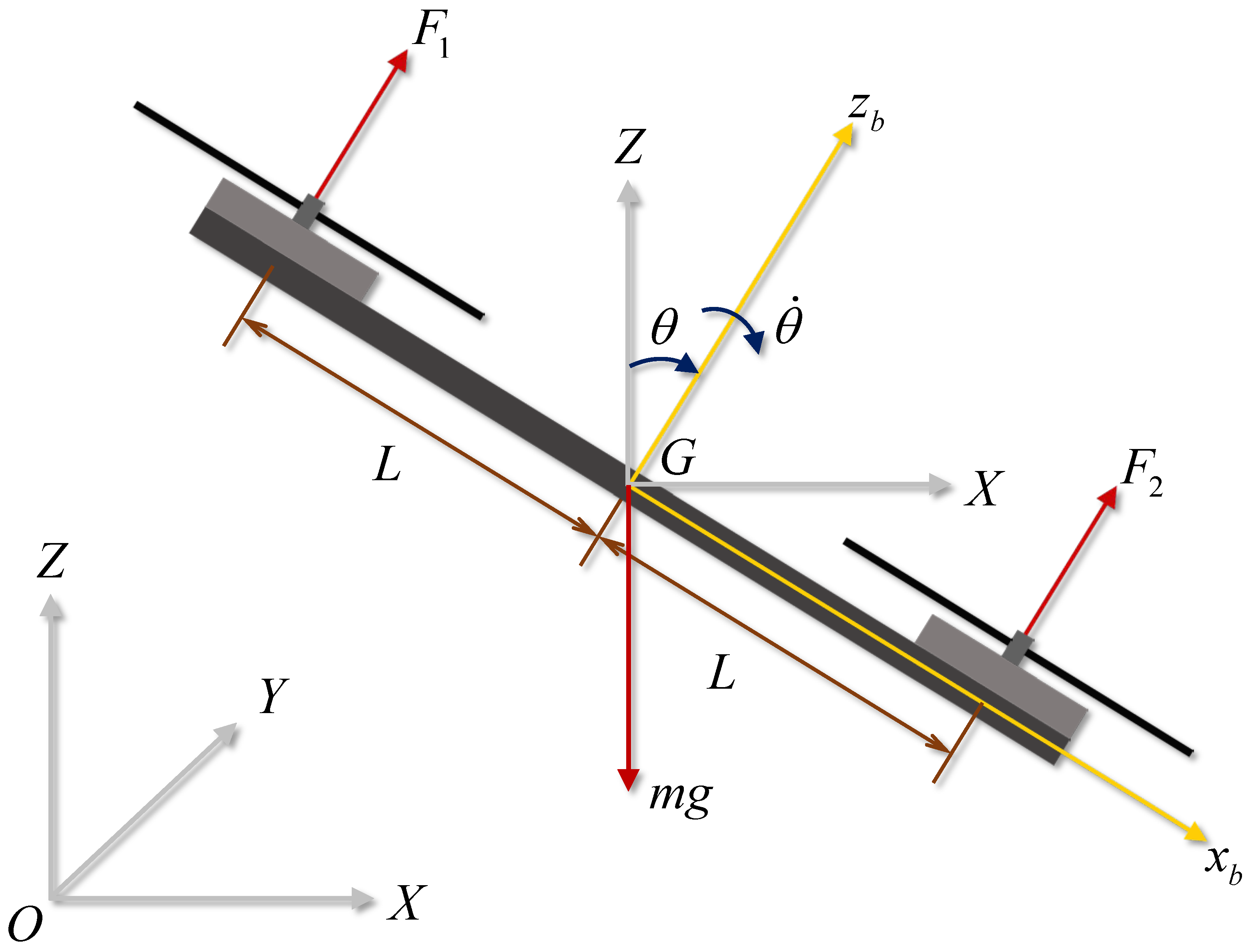
2. Dynamics Modeling
3. Flight Controller Design
3.1. Stability Analysis of General Error Dynamics
3.2. Altitude Proportional-Integral-Derivative Controller Design
3.3. Position Integral Backstepping Controller Design
3.4. Proposed Analytic Form of the Proposed Position Integral Backstepping Controller
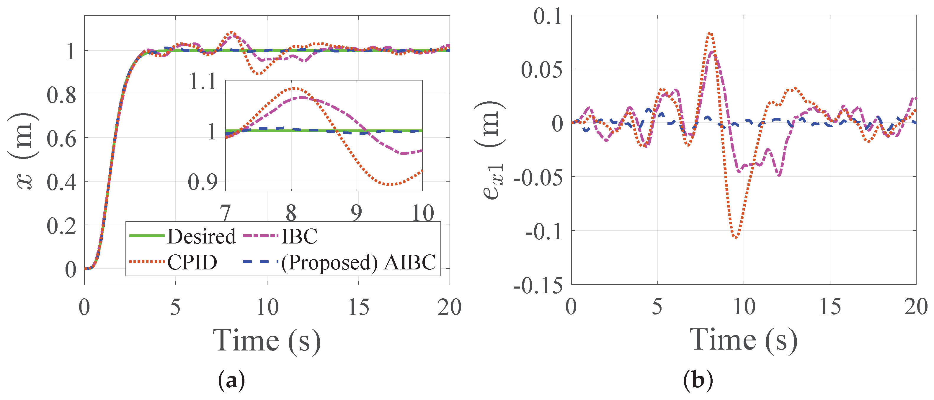
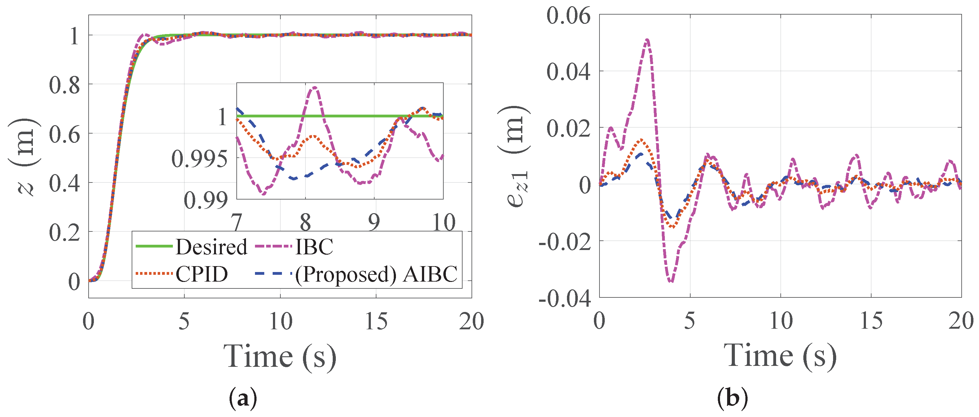
4. Numerical Simulations
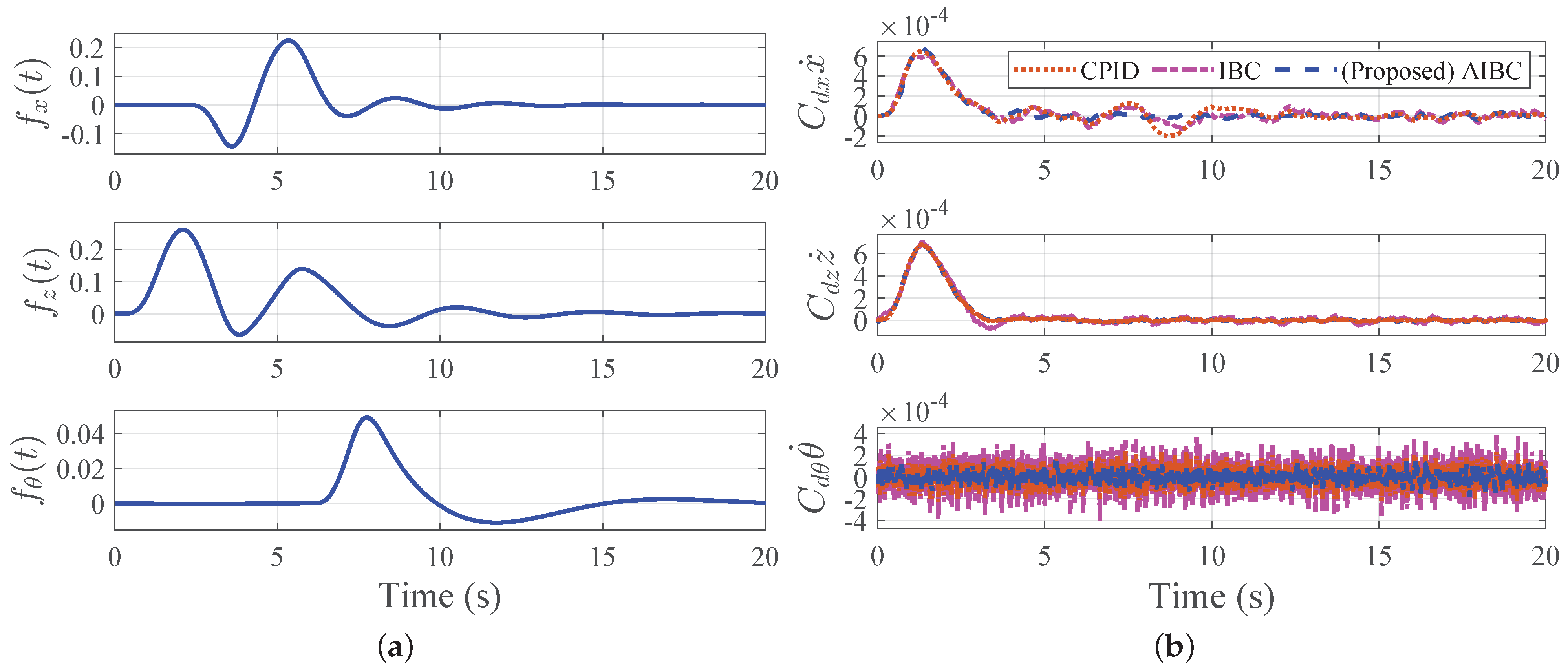
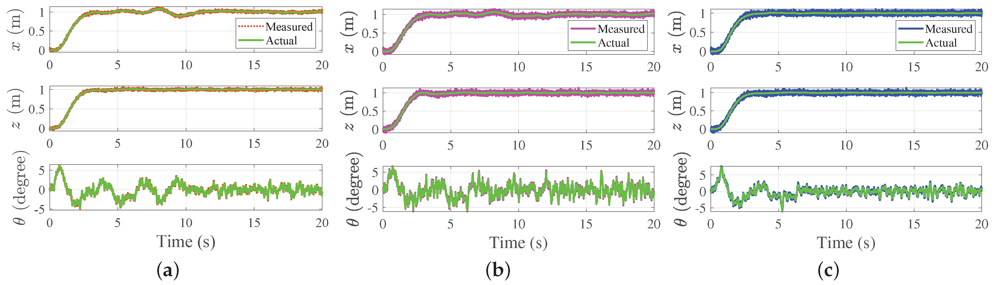
- Cascade PID controller (CPID). The cascade PID control presented in Appendix A is used;
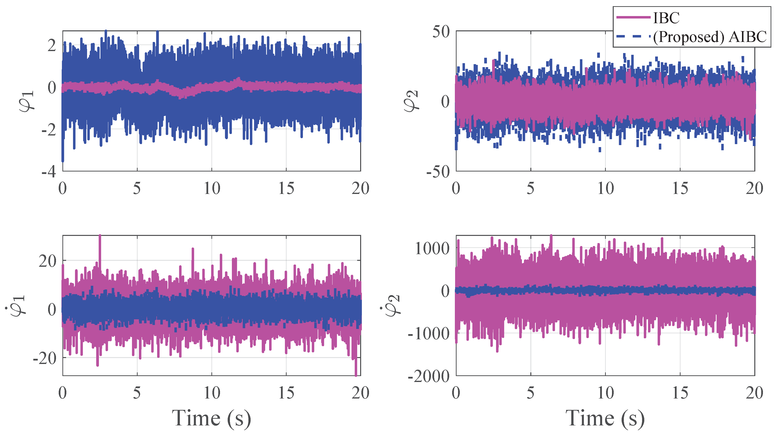
- Integral backstepping controller (IBC). The position integral backstepping controller derived from Theorem 2 is used, where the time derivatives of the virtual controls, and , are calculated by the approximated differentiator (APD) as illustrated in Appendix A;
- Analytic integral backstepping controller (AIBC). The proposed analytic integral backstepping controller presented in Theorem 3 is applied.
- 1.
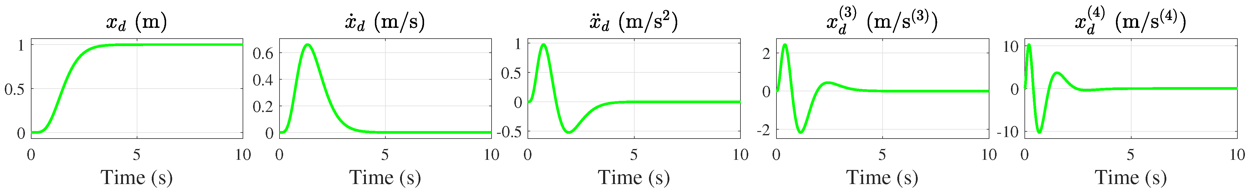
- Given the desired position and altitude trajectory , , and their successive derivatives, and ;
- 2.
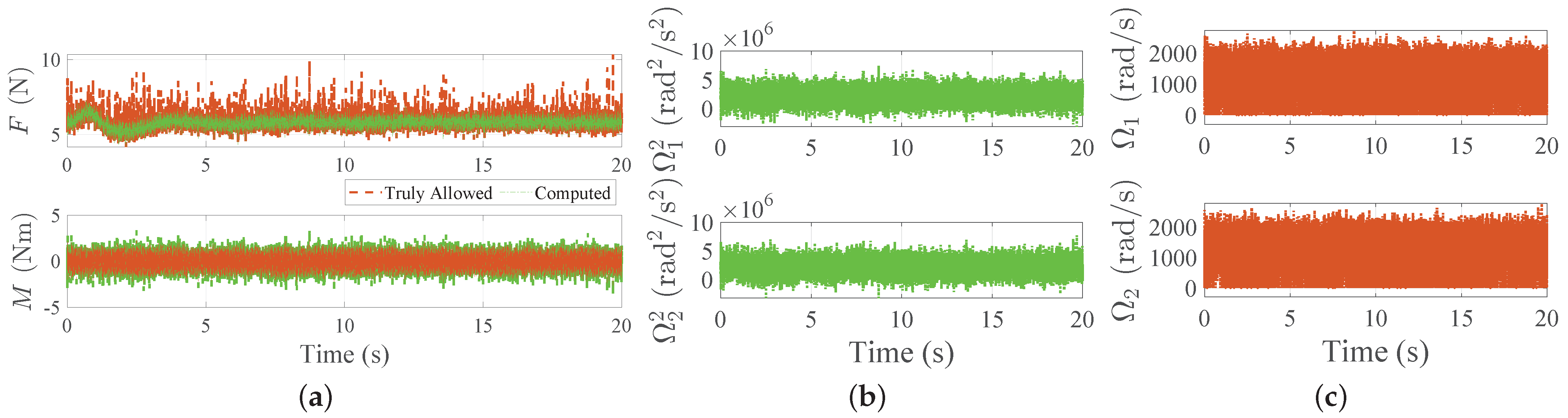
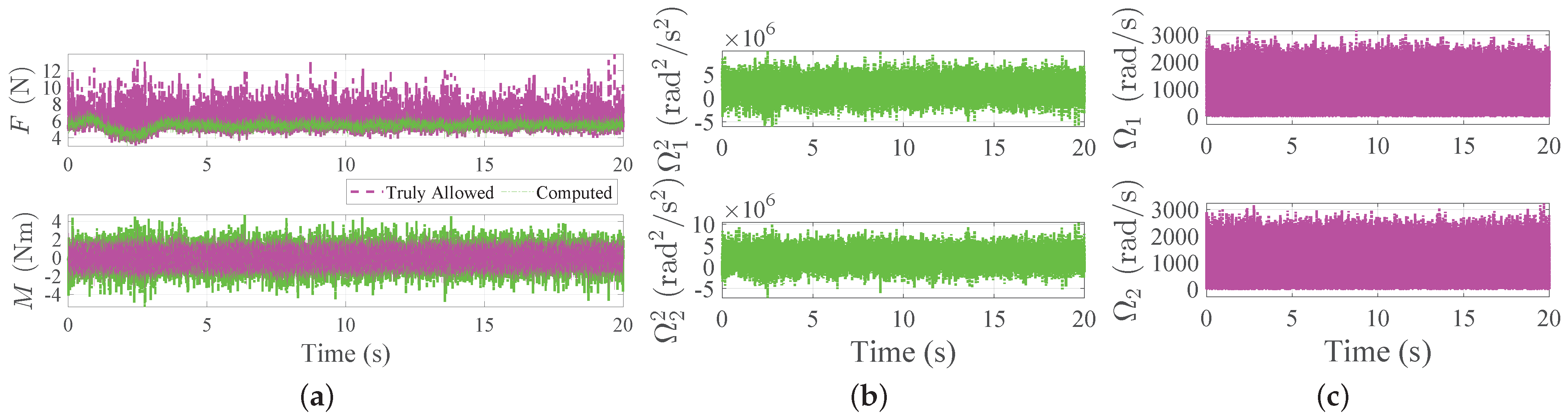
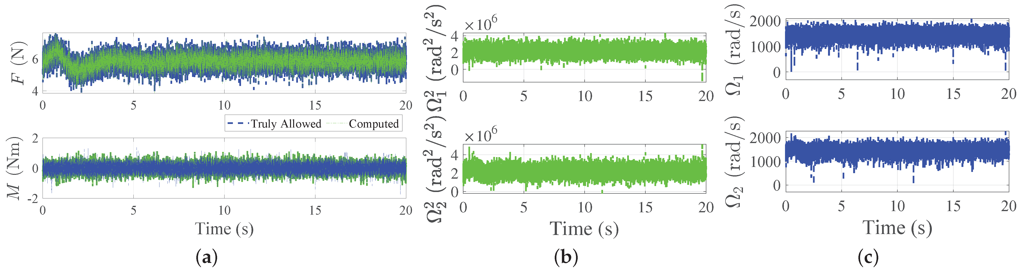
- Given the control gain pair , then determine the control force F from (37);
- 3.
- Determine the control torque M:
- (a)
- (b)
- (c)
- 4.
- Based on the calculated control force and control torque, compute the desired motor speed from (2);
- 5.
- Feed the desired speed to BLDC to generate the computed controls .
5. Conclusions
Author Contributions
Funding
Data Availability Statement
Conflicts of Interest
Appendix A. Derivation of Conventional Cascade PID Flight Controller
Appendix B. Existence Proof of Sliding Mode
References
- Bashi, O.I.D.; Hasan, W.; Azis, N.; Shafie, S.; Wagatsuma, H. Unmanned aerial vehicle quadcopter: A review. J. Comput. Theor. Nanosci. 2017, 14, 5663–5675. [Google Scholar] [CrossRef]
- Penicka, R.; Scaramuzza, D. Minimum-Time Quadrotor Waypoint Flight in Cluttered Environments. IEEE Robot. Autom. Lett. 2022, 7, 5719–5726. [Google Scholar] [CrossRef]
- Zhou, B.; Pan, J.; Gao, F.; Shen, S. RAPTOR: Robust and Perception-Aware Trajectory Replanning for Quadrotor Fast Flight. IEEE Trans. Robot. 2021, 37, 1992–2009. [Google Scholar] [CrossRef]
- Peng, C.C.; Cheng-Yu, W. Design of Constrained Dynamic Path Planning Algorithms in Large-Scale 3D Point Cloud Maps for UAVs. J. Comput. Sci. 2023, 67, 101944. [Google Scholar] [CrossRef]
- Falanga, D.; Kleber, K.; Scaramuzza, D. Dynamic obstacle avoidance for quadrotors with event cameras. Sci. Robot. 2020, 5, eaaz9712. [Google Scholar] [CrossRef]
- Yañez-Badillo, H.; Beltran-Carbajal, F.; Tapia-Olvera, R.; Favela-Contreras, A.; Sotelo, C.; Sotelo, D. Adaptive Robust Motion Control of Quadrotor Systems Using Artificial Neural Networks and Particle Swarm Optimization. Mathematics 2021, 9, 2367. [Google Scholar] [CrossRef]
- Nettari, Y.; Labbadi, M.; Kurt, S. Adaptive Robust Finite-Time Tracking Control for Quadrotor Subject to Disturbances. Adv. Space Res. 2022, in press. [CrossRef]
- Betancourt, J.; Castillo, P.; Garcia, P.; Balaguer, V.; Lozano, R. Robust bounded control scheme for quadrotor vehicles under high dynamic disturbances. preprint 2022. [CrossRef]
- Madani, T.; Benallegue, A. Backstepping control for a quadrotor helicopter. In Proceedings of the 2006 IEEE/RSJ International Conference on Intelligent Robots and Systems, Beijing, China, 9–15 October 2006; pp. 3255–3260. [Google Scholar] [CrossRef]
- Jasim, W.; Gu, D. Integral backstepping controller for quadrotor path tracking. In Proceedings of the 2015 International Conference on Advanced Robotics (ICAR), Istanbul, Turkey, 27–31 July 2015; pp. 593–598. [Google Scholar] [CrossRef]
- Zhou, L.; Zhang, J.; She, H.; Jin, H. Quadrotor UAV flight control via a novel saturation integral backstepping controller. Automatika 2019, 60, 193–206. [Google Scholar] [CrossRef]
- Labbadi, M.; Cherkaoui, M. Robust adaptive backstepping fast terminal sliding mode controller for uncertain quadrotor UAV. Aerosp. Sci. Technol. 2019, 93, 105306. [Google Scholar] [CrossRef]
- Koksal, N.; An, H.; Fidan, B. Backstepping-based adaptive control of a quadrotor UAV with guaranteed tracking performance. ISA Trans. 2020, 105, 98–110. [Google Scholar] [CrossRef] [PubMed]
- Xuan-Mung, N.; Hong, S.K. Robust Backstepping Trajectory Tracking Control of a Quadrotor with Input Saturation via Extended State Observer. Appl. Sci. 2019, 9, 5184. [Google Scholar] [CrossRef] [Green Version]
- Govea-Vargas, A.; Castro-Linares, R.; Duarte-Mermoud, M.A.; Aguila-Camacho, N.; Ceballos-Benavides, G.E. Fractional Order Sliding Mode Control of a Class of Second Order Perturbed Nonlinear Systems: Application to the Trajectory Tracking of a Quadrotor. Algorithms 2018, 11, 168. [Google Scholar] [CrossRef] [Green Version]
- Niu, Y.; Ban, H.; Zhang, H.; Gong, W.; Yu, F. Nonsingular Terminal Sliding Mode Based Finite-Time Dynamic Surface Control for a Quadrotor UAV. Algorithms 2021, 14, 315. [Google Scholar] [CrossRef]
- Zhao, J.; Wang, X.; Gao, G.; Na, J.; Liu, H.; Luan, F. Online Adaptive Parameter Estimation for Quadrotors. Algorithms 2018, 11, 167. [Google Scholar] [CrossRef] [Green Version]
- Liu, J.; Gai, W.; Zhang, J.; Li, Y. Nonlinear adaptive backstepping with ESO for the quadrotor trajectory tracking control in the multiple disturbances. Int. J. Control. Autom. Syst. 2019, 17, 2754–2768. [Google Scholar] [CrossRef]
- Chovancová, A.; Fico, T.; Chovanec, Ľ.; Hubinsk, P. Mathematical Modelling and Parameter Identification of Quadrotor (a survey). Procedia Eng. 2014, 96, 172–181. [Google Scholar] [CrossRef] [Green Version]
- Ventura Diaz, P.; Yoon, S. High-fidelity computational aerodynamics of multi-rotor unmanned aerial vehicles. In Proceedings of the 2018 AIAA Aerospace Sciences Meeting, Kissimmee, FL, USA, 8–12 January 2018; p. 1266. [Google Scholar]
- Moreno-Valenzuela, J.; Pérez-Alcocer, R.; Guerrero-Medina, M.; Dzul, A. Nonlinear PID-Type Controller for Quadrotor Trajectory Tracking. IEEE/ASME Trans. Mechatron. 2018, 23, 2436–2447. [Google Scholar] [CrossRef]
- Jia, Z.; Yu, J.; Mei, Y.; Chen, Y.; Shen, Y.; Ai, X. Integral Backstepping Sliding Mode Control for Quadrotor Helicopter under External Uncertain Disturbances. Aerosp. Sci. Technol. 2017, 68, 299–307. [Google Scholar] [CrossRef]
- Ríos, H.; Falcón, R.; González, O.A.; Dzul, A. Continuous Sliding-Mode Control Strategies for Quadrotor Robust Tracking: Real-Time Application. IEEE Trans. Ind. Electron. 2019, 66, 1264–1272. [Google Scholar] [CrossRef]
- Zhang, Z.; Wang, F.; Guo, Y.; Hua, C. Multivariable sliding mode backstepping controller design for quadrotor UAV based on disturbance observer. Sci. China Inf. Sci. 2018, 61, 1–16. [Google Scholar] [CrossRef] [Green Version]
- Goodarzi, F.; Lee, D.; Lee, T. Geometric nonlinear PID control of a quadrotor UAV on SE(3). In Proceedings of the 2013 European Control Conference (ECC), Zurich, Switzerland, 17–19 July 2013; pp. 3845–3850. [Google Scholar] [CrossRef] [Green Version]
- Demirhan, M.; Premachandra, C. Development of an Automated Camera-Based Drone Landing System. IEEE Access 2020, 8, 202111–202121. [Google Scholar] [CrossRef]
- Piponidis, M.; Aristodemou, P.; Theocharides, T. Towards a Fully Autonomous UAV Controller for Moving Platform Detection and Landing. In Proceedings of the 2022 35th International Conference on VLSI Design and 2022 21st International Conference on Embedded Systems (VLSID), Bangalore, India, 26 February–2 March 2022; pp. 180–185. [Google Scholar] [CrossRef]
- Peng, C.C.; Li, Y.; Chen, C.L. A robust integral type backstepping controller design for control of uncertain nonlinear systems subject to disturbance. Int. J. Innov. Comput. Inf. Control 2011, 7, 2543–2560. [Google Scholar]
- Meslouli, I.; Kahouadji, M.; Choukchou-Braham, A.; Bensalah, C.; Mokhtari, M.R.; Cherki, B. Experimental validation of quaternion based integral backstepping design for attitude tracking. In Proceedings of the 2018 6th International Conference on Control Engineering & Information Technology (CEIT), Istanbul, Turkey, 25–27 October 2018; pp. 1–6. [Google Scholar] [CrossRef]
- Peng, C.C.; Chen, T.Y. A recursive low-pass filtering method for a commercial cooling fan tray parameter online estimation with measurement noise. Measurement 2022, 205, 112193. [Google Scholar] [CrossRef]
- Peng, C.C.; Su, C.Y. Modeling and Parameter Identification of a Cooling Fan for Online Monitoring. IEEE Trans. Instrum. Meas. 2021, 70, 1–14. [Google Scholar] [CrossRef]
- Zhang, F. The Schur Complement and Its Applications; Springer Science & Business Media: Berlin/Heidelberg, Germany, 2006; Volume 4. [Google Scholar]
- Aguilar-Ibañez, C. Stabilization of the PVTOL aircraft based on a sliding mode and a saturation function. Int. J. Robust Nonlinear Control. 2017, 27, 843–859. [Google Scholar] [CrossRef]
- Shi, Z.; Deng, C.; Zhang, S.; Xie, Y.; Cui, H.; Hao, Y. Hyperbolic Tangent Function-Based Finite-Time Sliding Mode Control for Spacecraft Rendezvous Maneuver Without Chattering. IEEE Access 2020, 8, 60838–60849. [Google Scholar] [CrossRef]
- Khandekar, A.A.; Malwatkar, G.M.; Patre, B.M. Discrete Sliding Mode Control for Robust Tracking of Higher Order Delay Time Systems with Experimental Application. ISA Trans. 2013, 52, 36–44. [Google Scholar] [CrossRef]
- Defoort, M.; Floquet, T.; Kokosy, A.; Perruquetti, W. A Novel Higher Order Sliding Mode Control Scheme. Syst. Control Lett. 2009, 58, 102–108. [Google Scholar] [CrossRef] [Green Version]


| Quantity | Description | Unit |
|---|---|---|
| m | Mass | kg |
| J | Moment of inertia | kg-m |
| g | Gravitational acceleration | m/s |
| L | Distance between motors and center of mass | m |
| m | L | J | g | , | |||
|---|---|---|---|---|---|---|---|
| Unit | kg | m | kg-m | N/(rad/s) | m/s | (N/(m/s) | N.m/(rad/s) |
| 0.6 | 0.25 | 9.8 |
| CPID | IBC | (Proposed) AIBC | |
|---|---|---|---|
| x-direction | 0.0314 | 0.0229 | 0.0037 |
| z-direction | 0.0055 | 0.0145 | 0.0043 |
Disclaimer/Publisher’s Note: The statements, opinions and data contained in all publications are solely those of the individual author(s) and contributor(s) and not of MDPI and/or the editor(s). MDPI and/or the editor(s) disclaim responsibility for any injury to people or property resulting from any ideas, methods, instructions or products referred to in the content. |
© 2023 by the authors. Licensee MDPI, Basel, Switzerland. This article is an open access article distributed under the terms and conditions of the Creative Commons Attribution (CC BY) license (https://creativecommons.org/licenses/by/4.0/).
Share and Cite
Li, Y.-R.; Chen, C.-C.; Peng, C.-C. Integral Backstepping Control Algorithm for a Quadrotor Positioning Flight Task: A Design Issue Discussion. Algorithms 2023, 16, 122. https://doi.org/10.3390/a16020122
Li Y-R, Chen C-C, Peng C-C. Integral Backstepping Control Algorithm for a Quadrotor Positioning Flight Task: A Design Issue Discussion. Algorithms. 2023; 16(2):122. https://doi.org/10.3390/a16020122
Chicago/Turabian StyleLi, Yang-Rui, Chih-Chia Chen, and Chao-Chung Peng. 2023. "Integral Backstepping Control Algorithm for a Quadrotor Positioning Flight Task: A Design Issue Discussion" Algorithms 16, no. 2: 122. https://doi.org/10.3390/a16020122