
Enhancing Sustainability of Corroded RC Structures: Estimating Steel-to-Concrete Bond Strength with ANN and SVM Algorithms

 ,
,  , and
, and
Abstract
:1. Introduction
1.1. Determination of BS
2. Application of ML in Concrete Technology
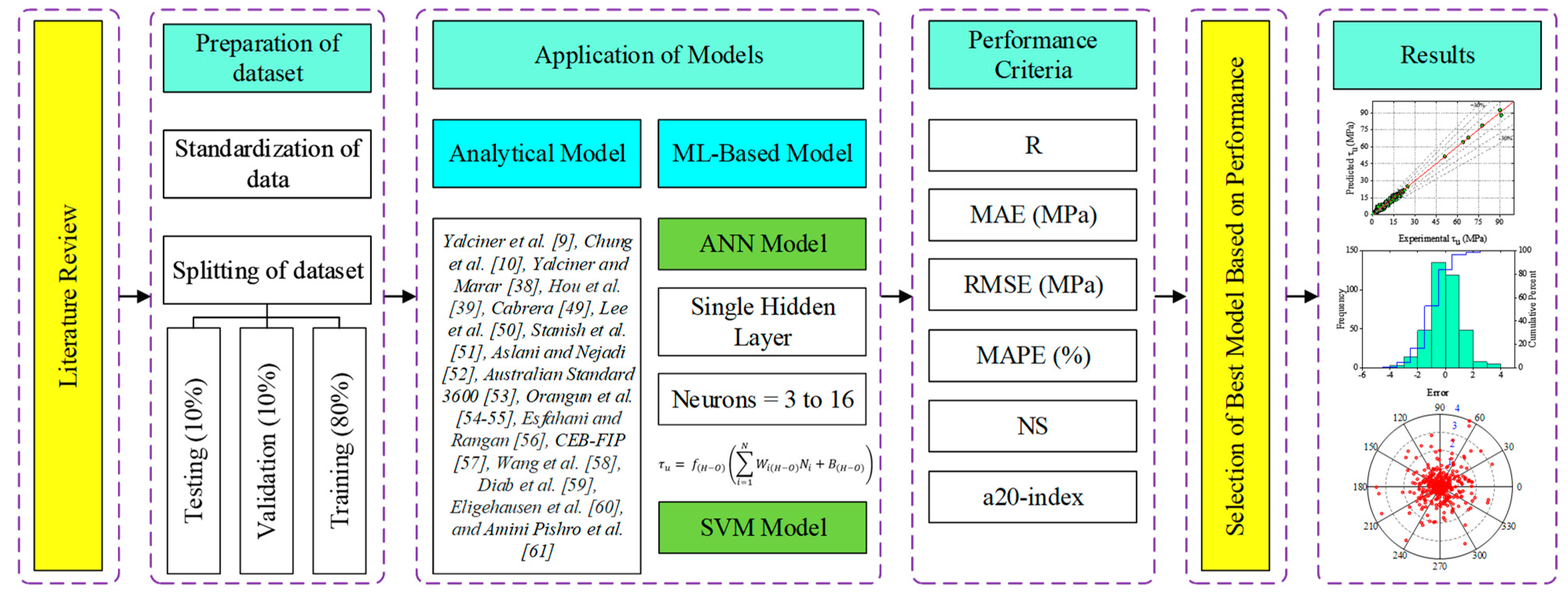
3. Experimental Data and Methods
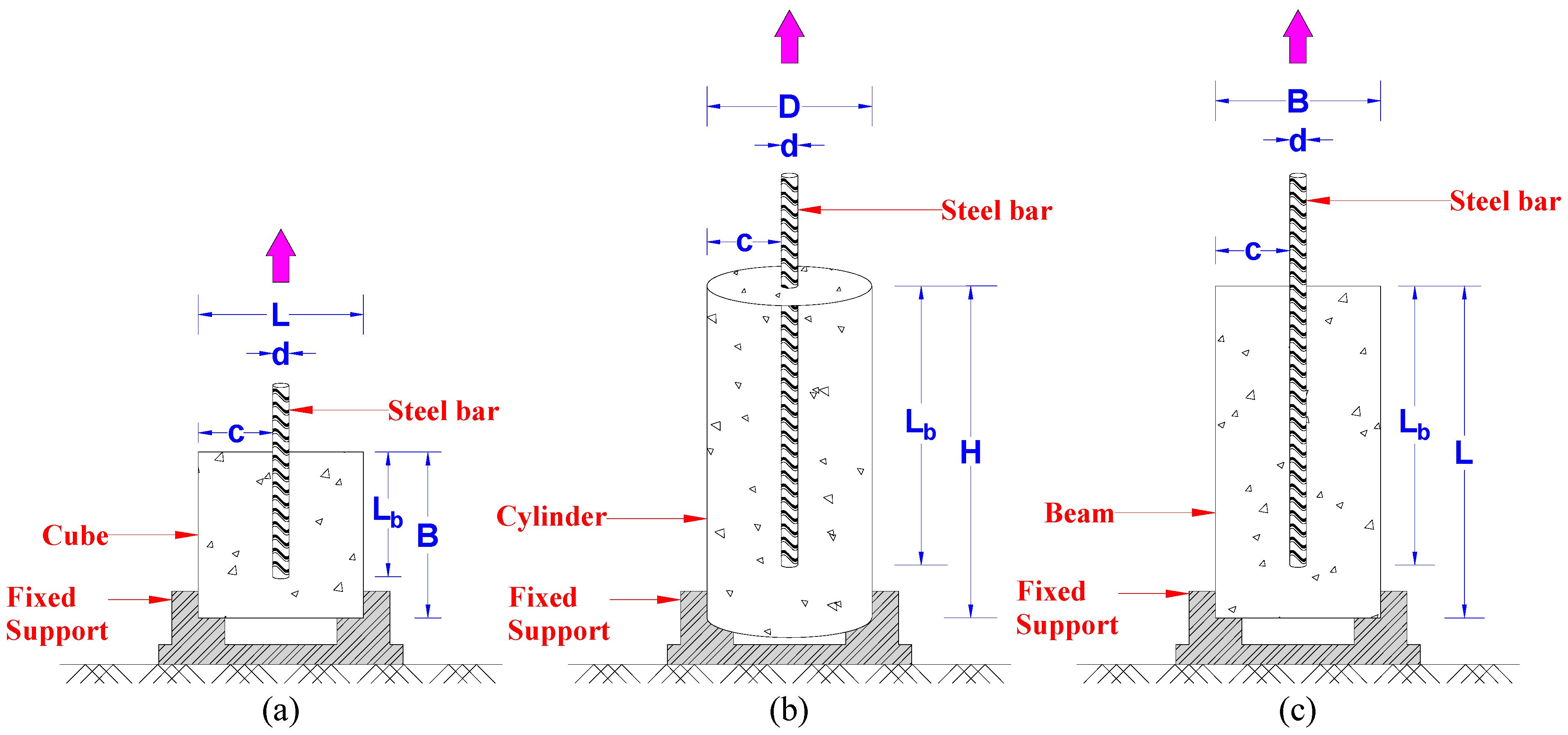
3.1. Data Bank
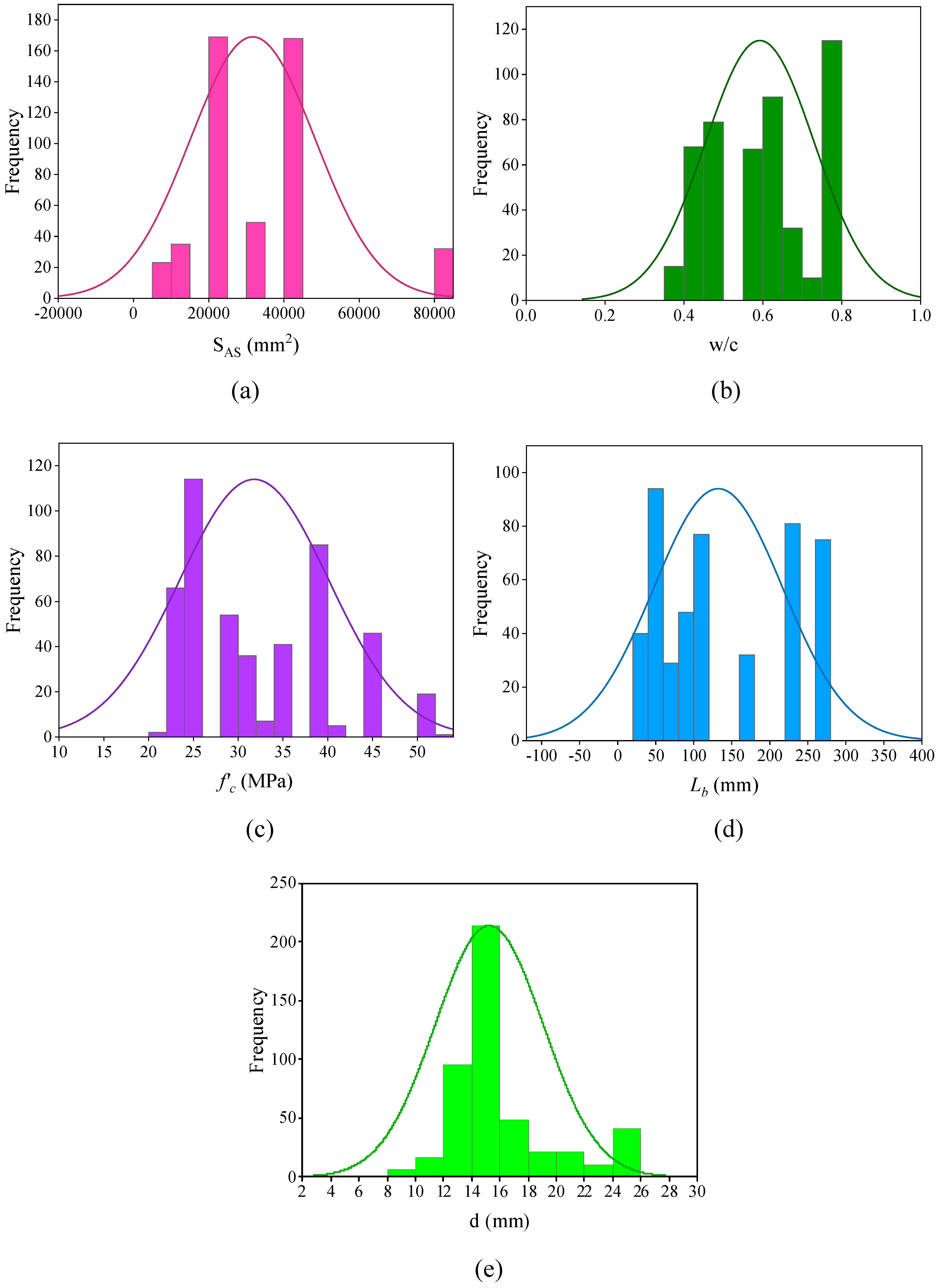
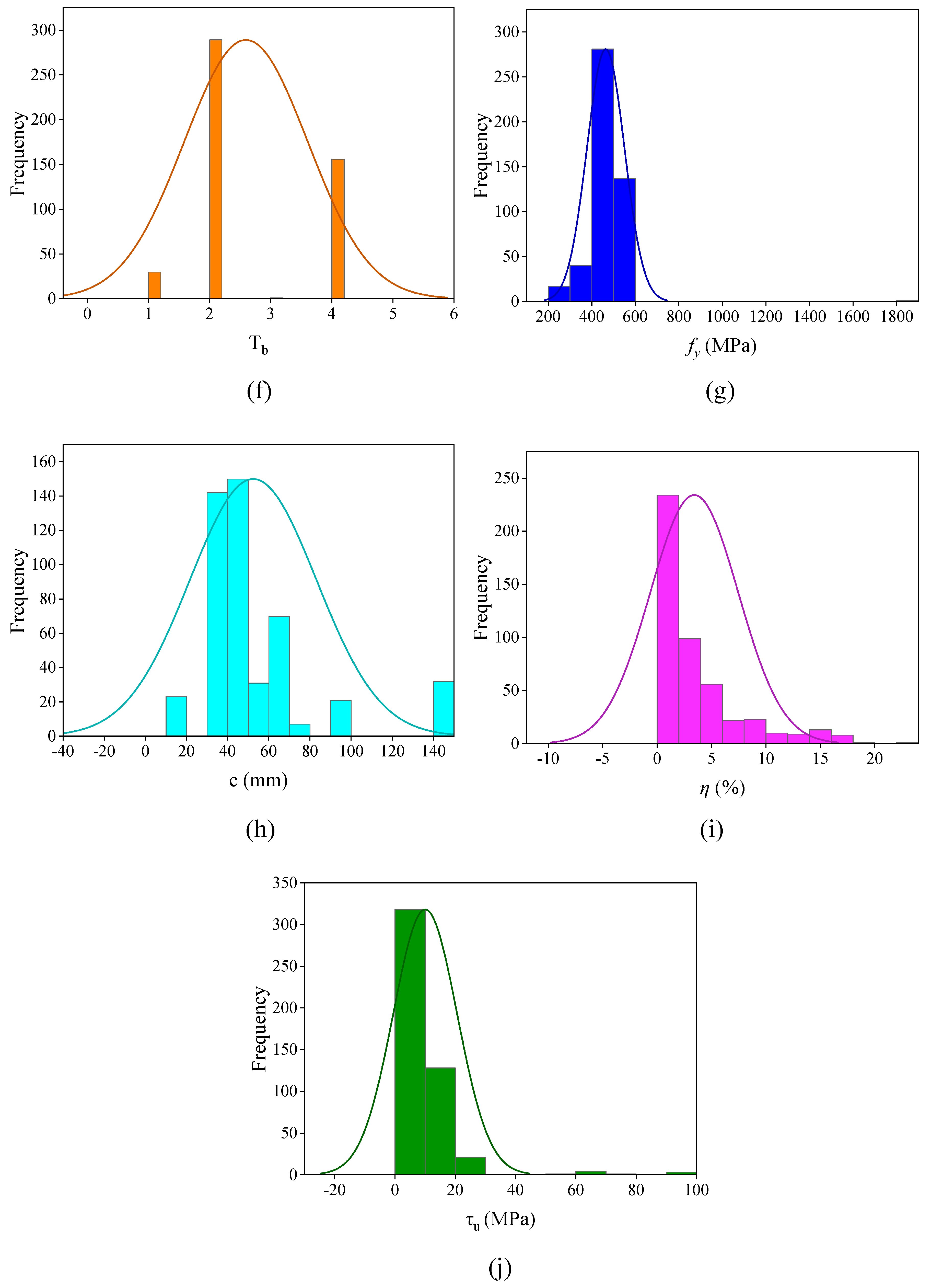
3.2. Preparation of Data
3.3. Performance Criterion
3.4. Analytical Models
4. ML
4.1. SVM
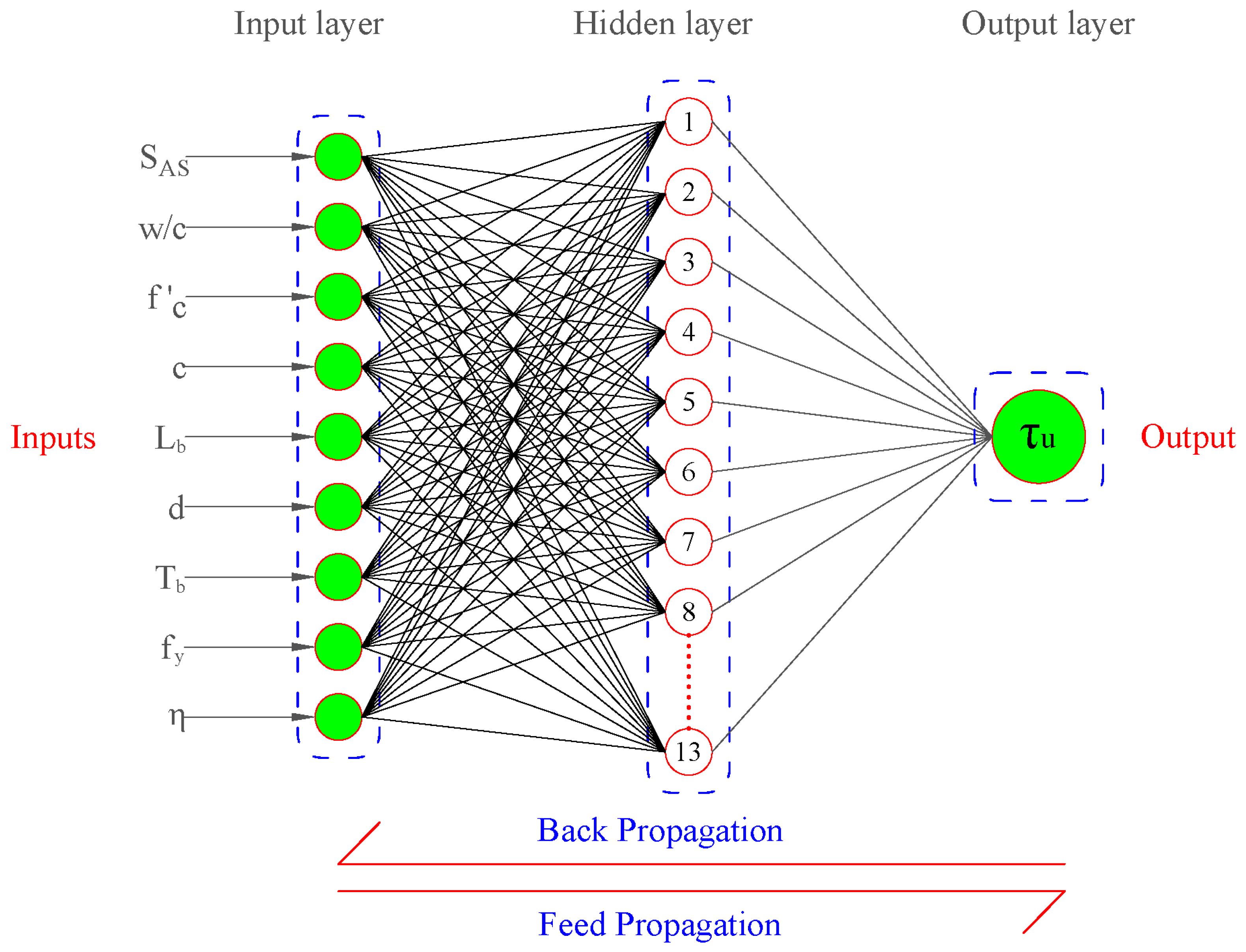
4.2. ANN
Development of ANN Model
5. Results and Discussion
5.1. Results of Analytical Models
5.2. Results of ANN and SVM Models
5.3. Discussion
5.4. Relative Importance
5.5. ANN Formulation
6. Conclusions
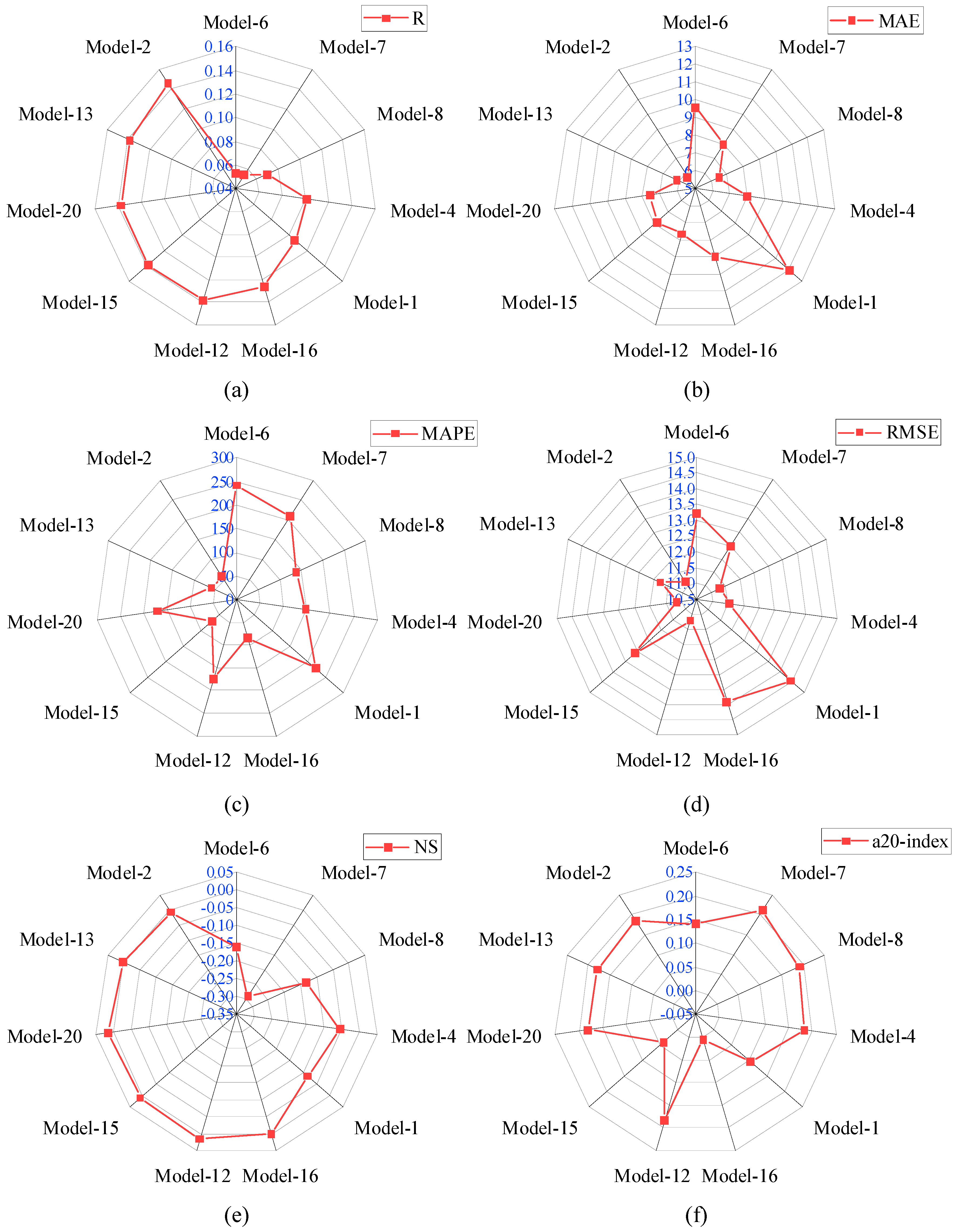
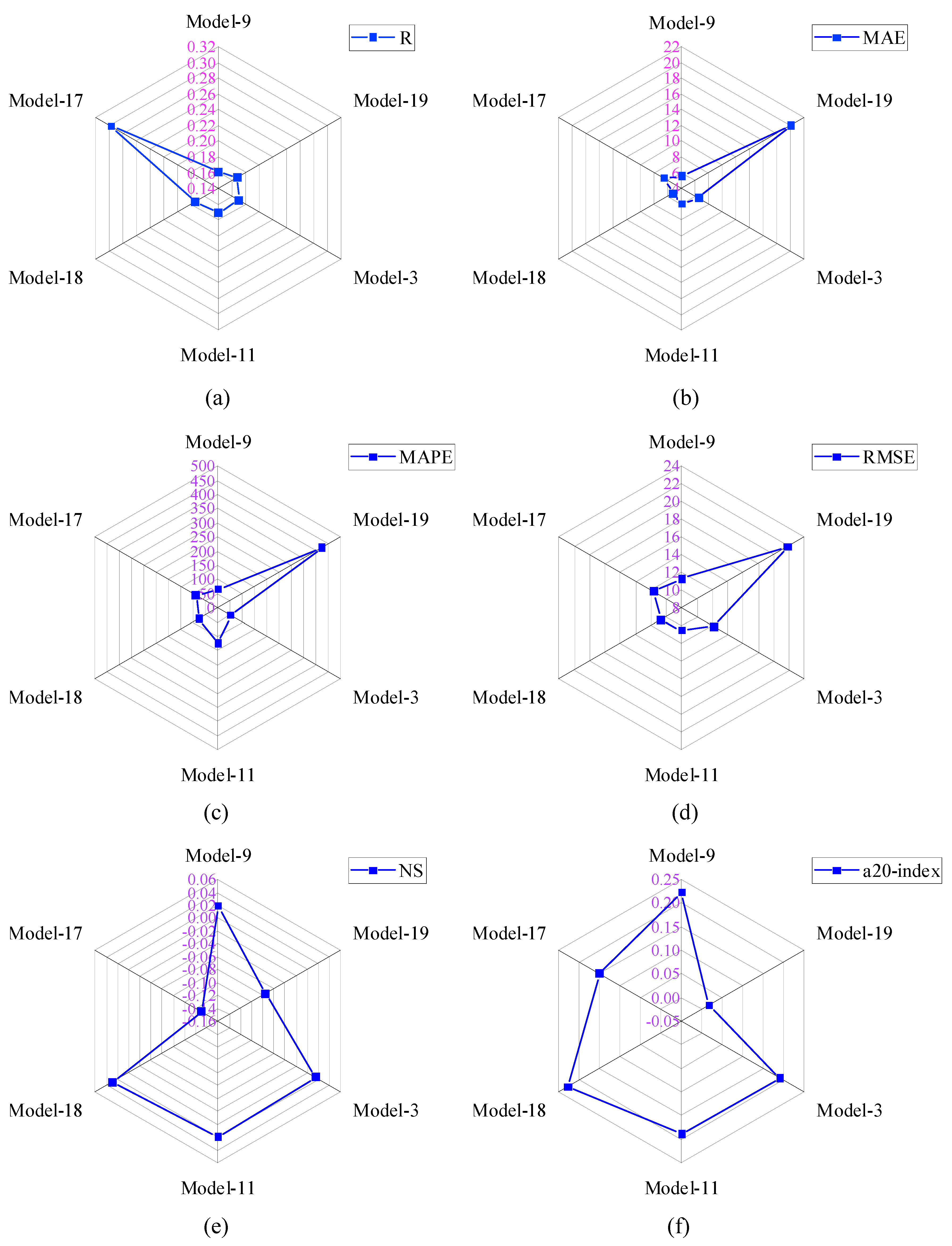
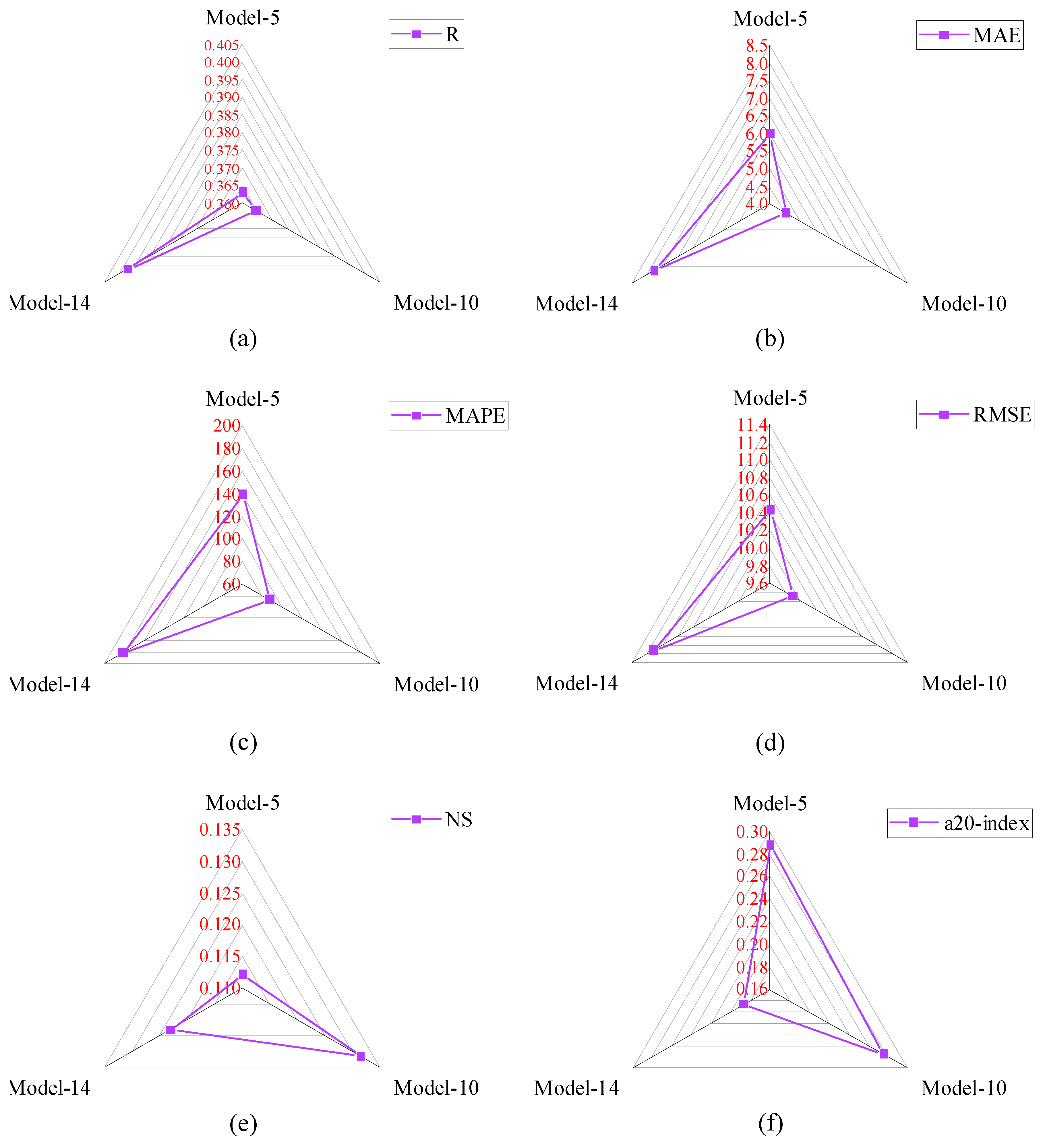
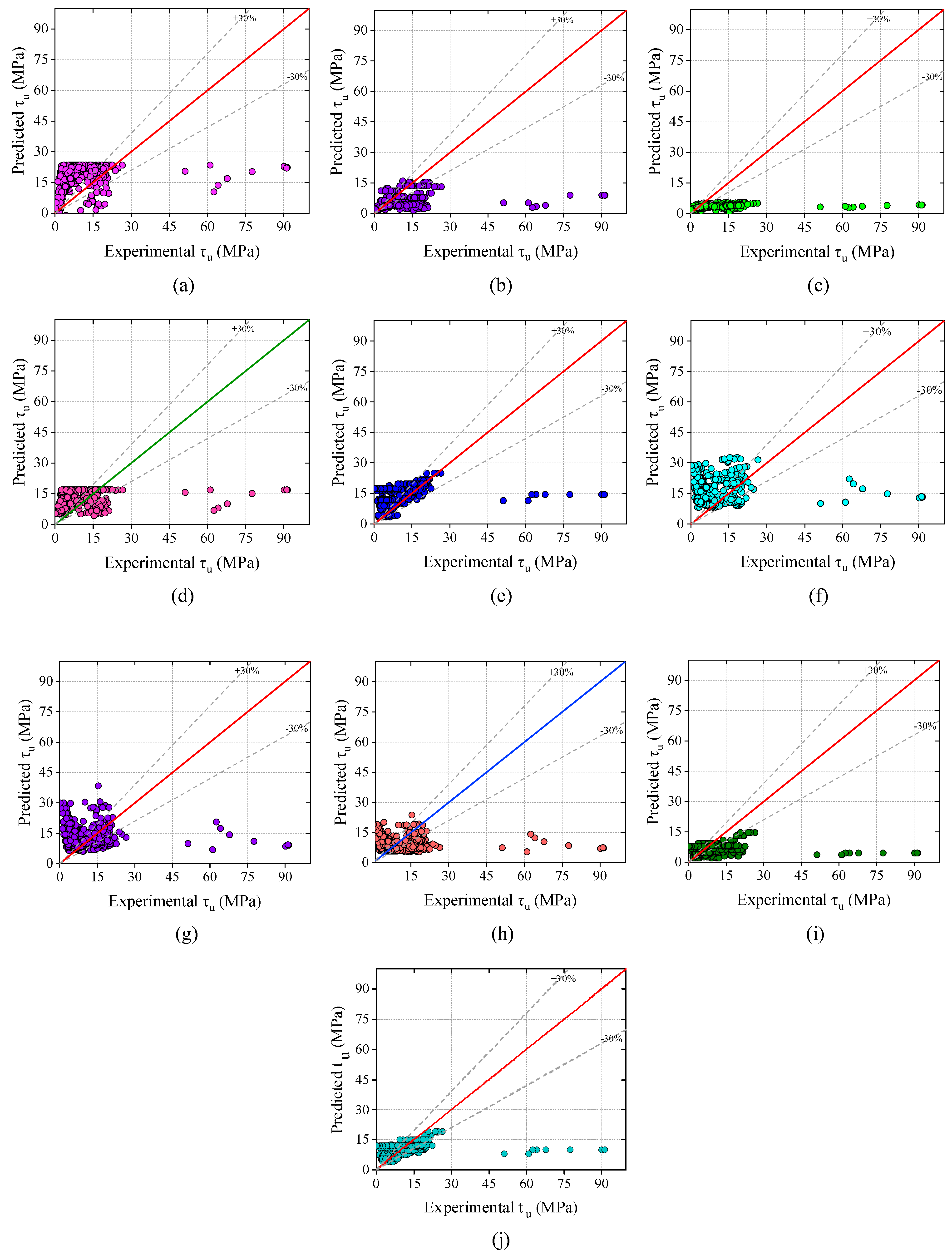
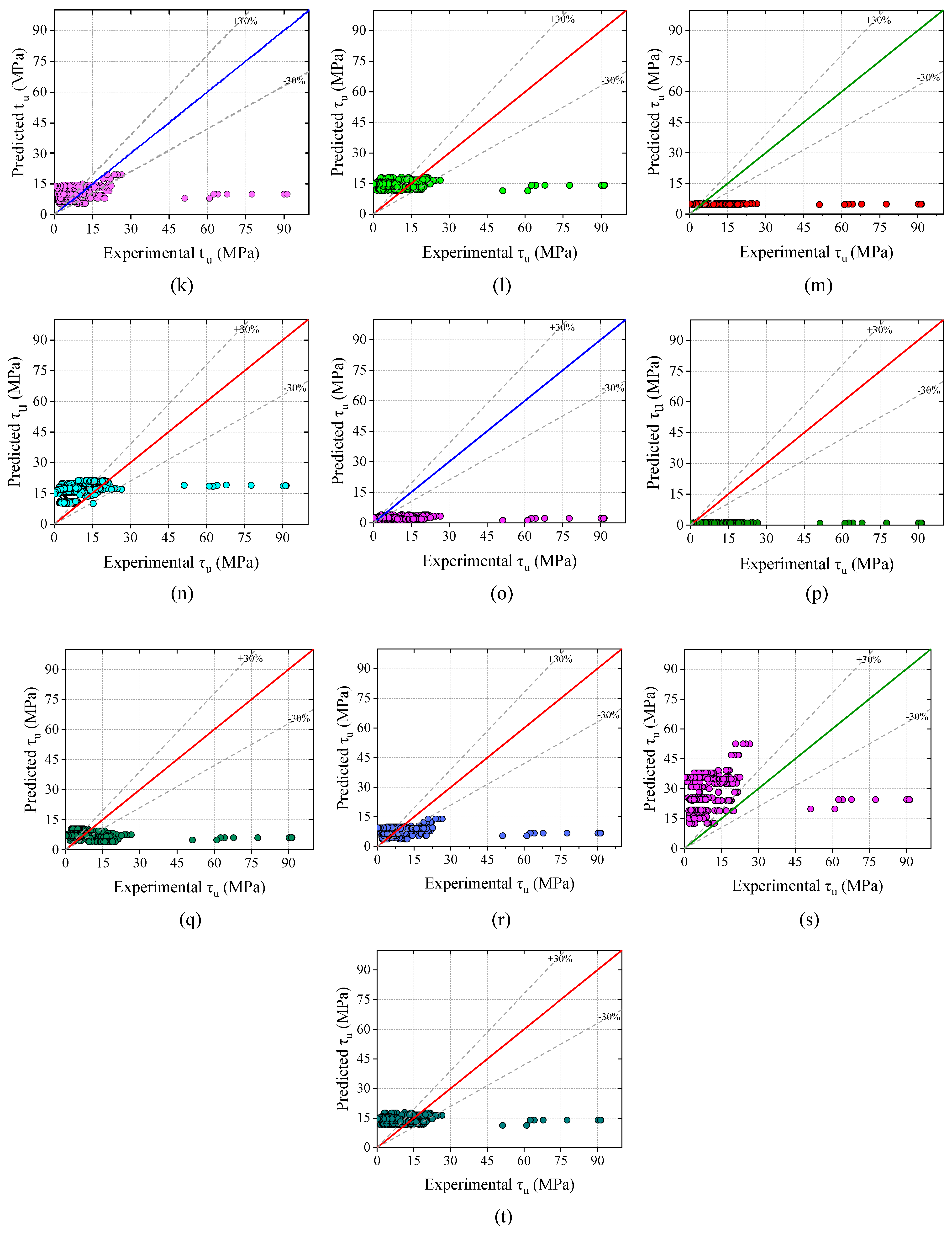
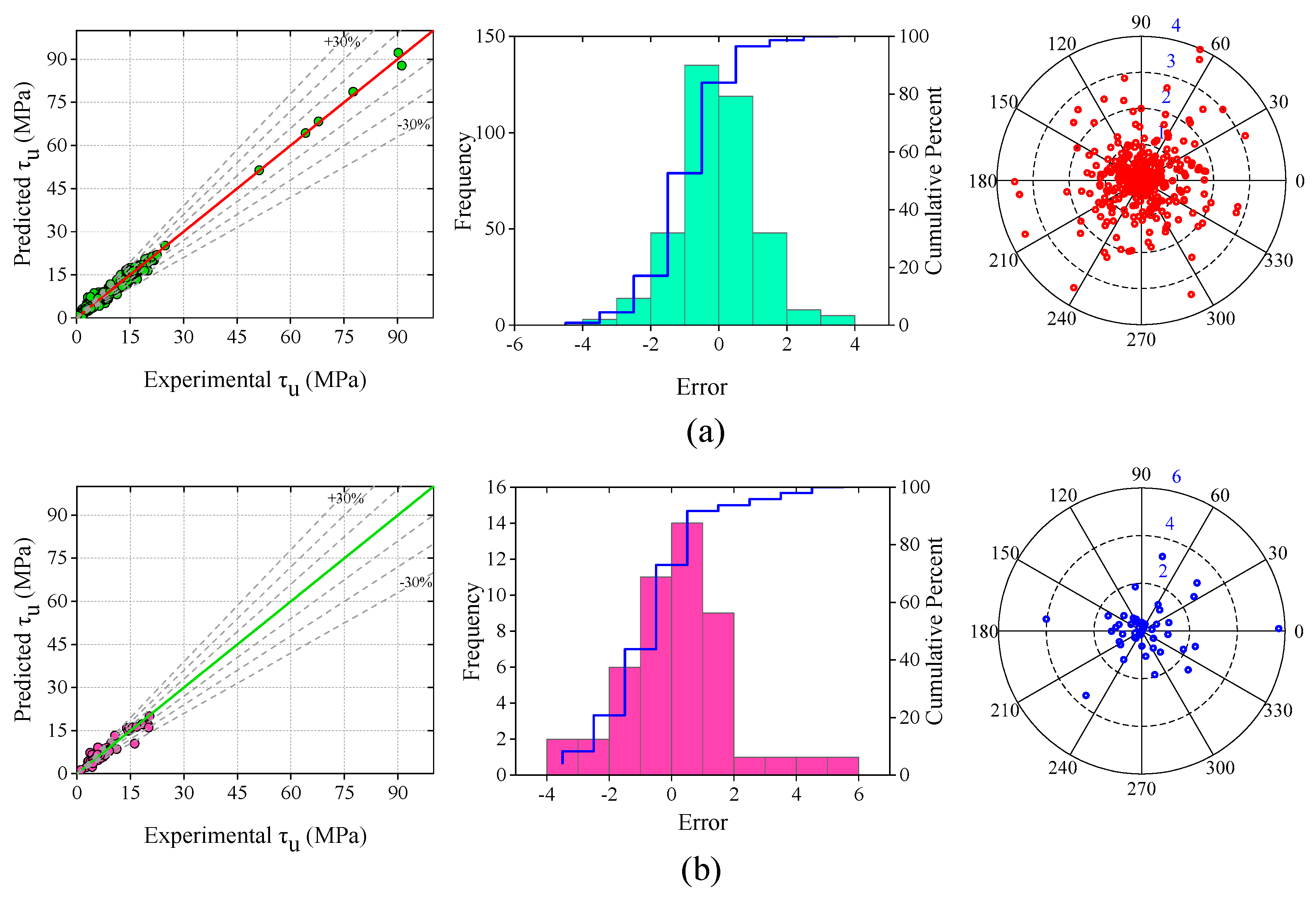
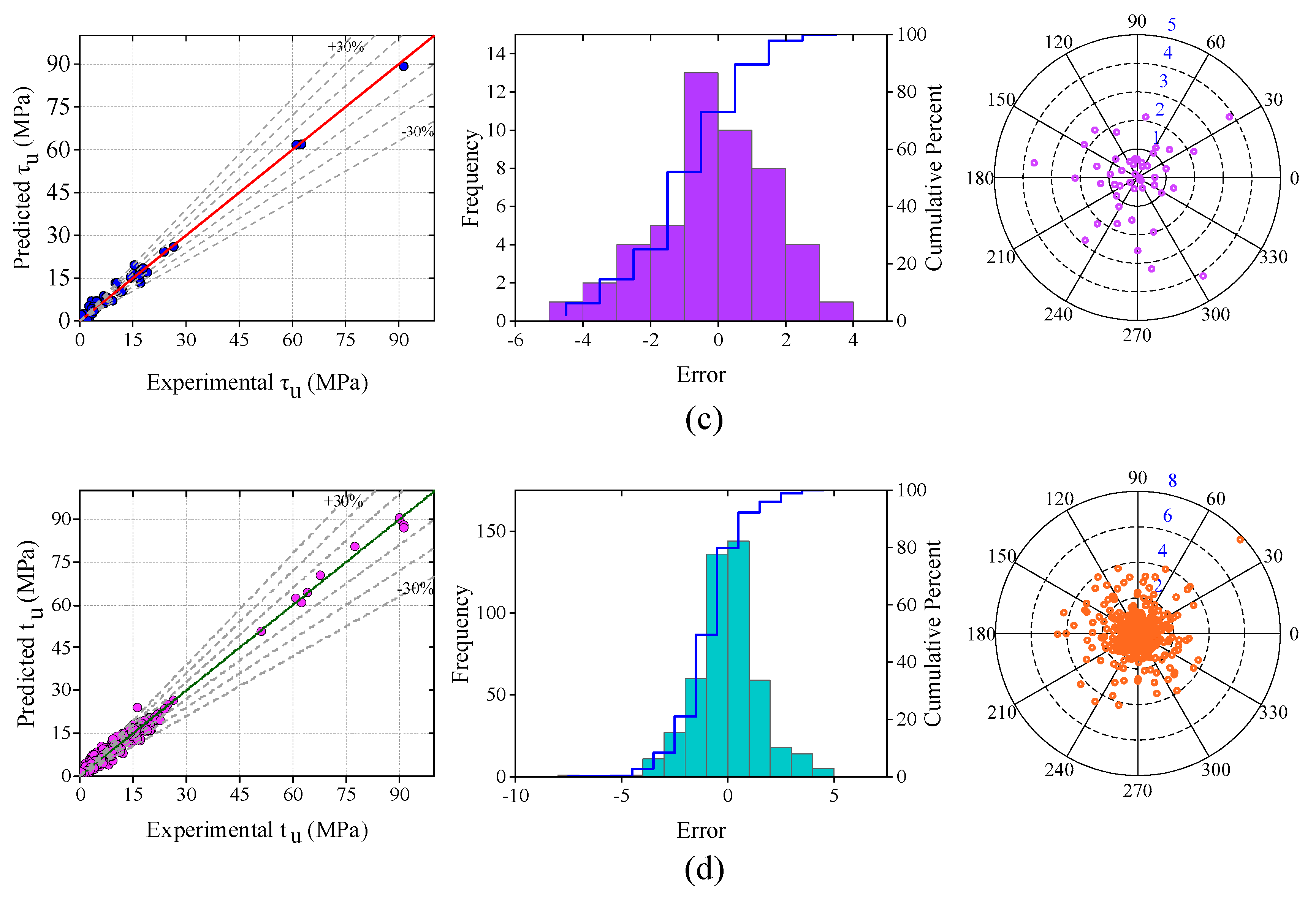
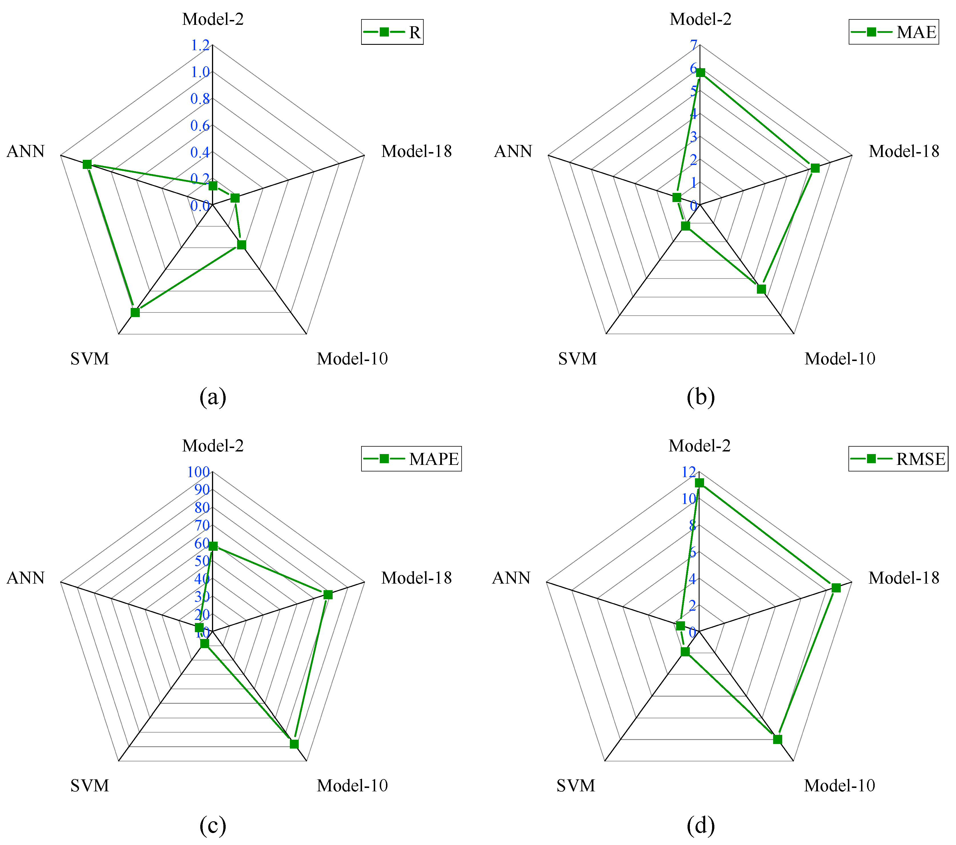
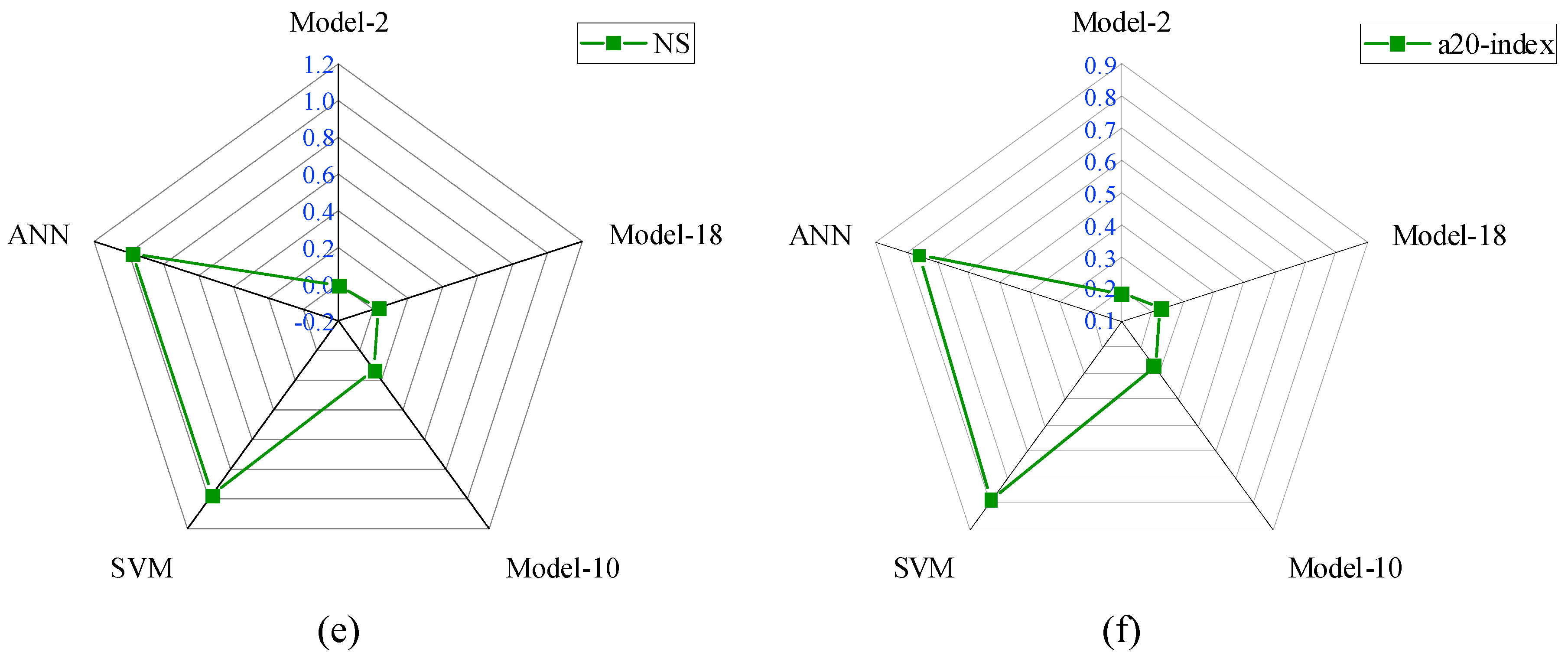
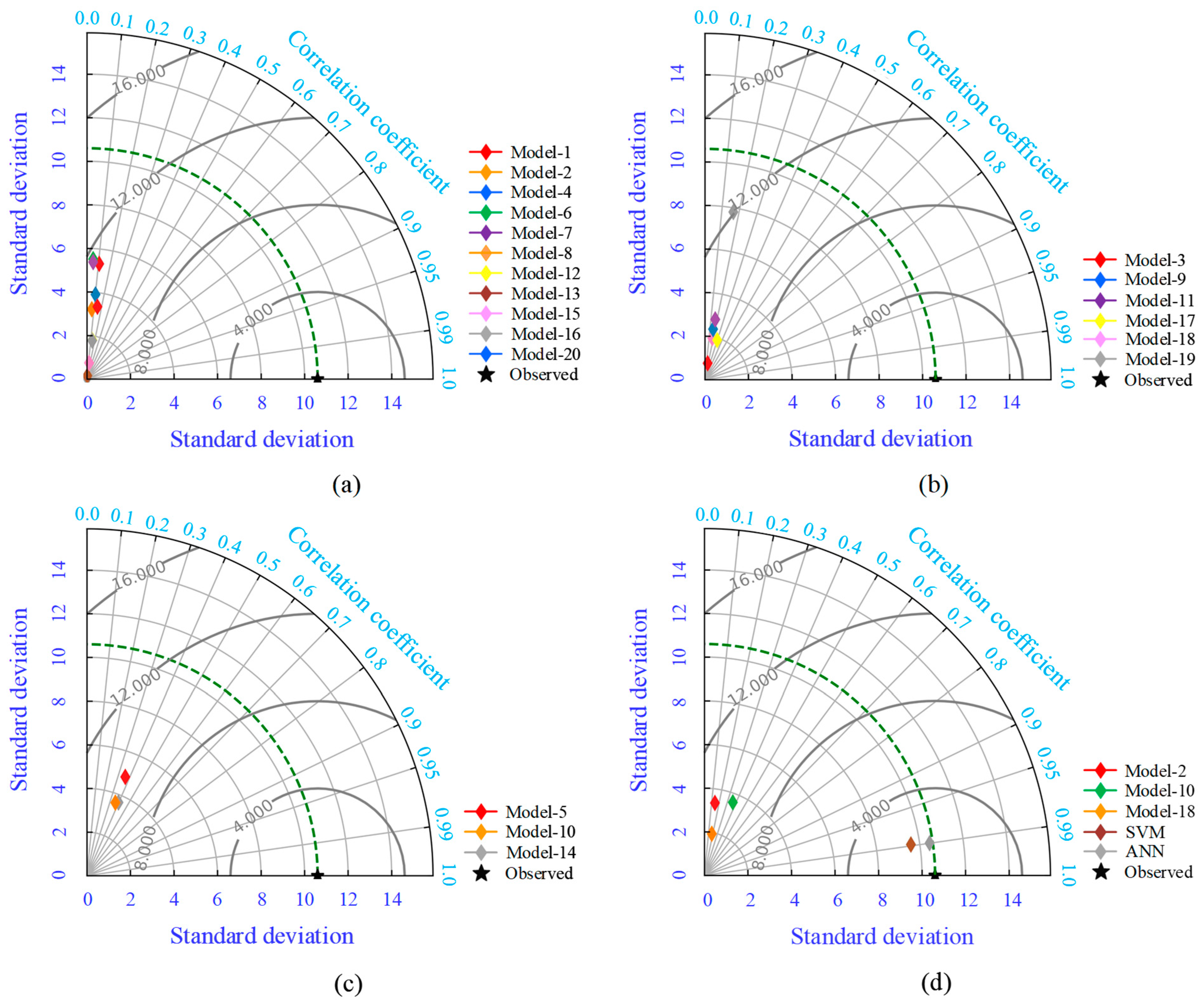
- Based on the R-value, twenty analytical models were divided into three groups Group-I, Group-II, and Group-III with R-ranges of 0 to 0.15, 0.15 to 0.30, and 0.30 to 0.40, respectively. Model-2 performed well in Group-I, with an R-value of 0.146. Similar to this, Model-18 performed well in Group II with an R-value of 0.174, while Model-10 performed well in Group III with an R-value of 0.364.
- The R-value of Model-10 was 149.32% and 109.2% higher than Model-2 and Model-18, respectively. The NS value of Model-10 was 351.72% higher than Model-18. Similarly, the a20-index of Model-10 was 48.65% and 20.09% higher than Model-2 and Model-18, respectively.
- The MAE and RMSE values of Model-10 were 4.514 MPa and 9.888 MPa, which were lowest among all the analytical models. In the analytical models, the performance of Model-10 was good compared with Group-I, II, and III models.
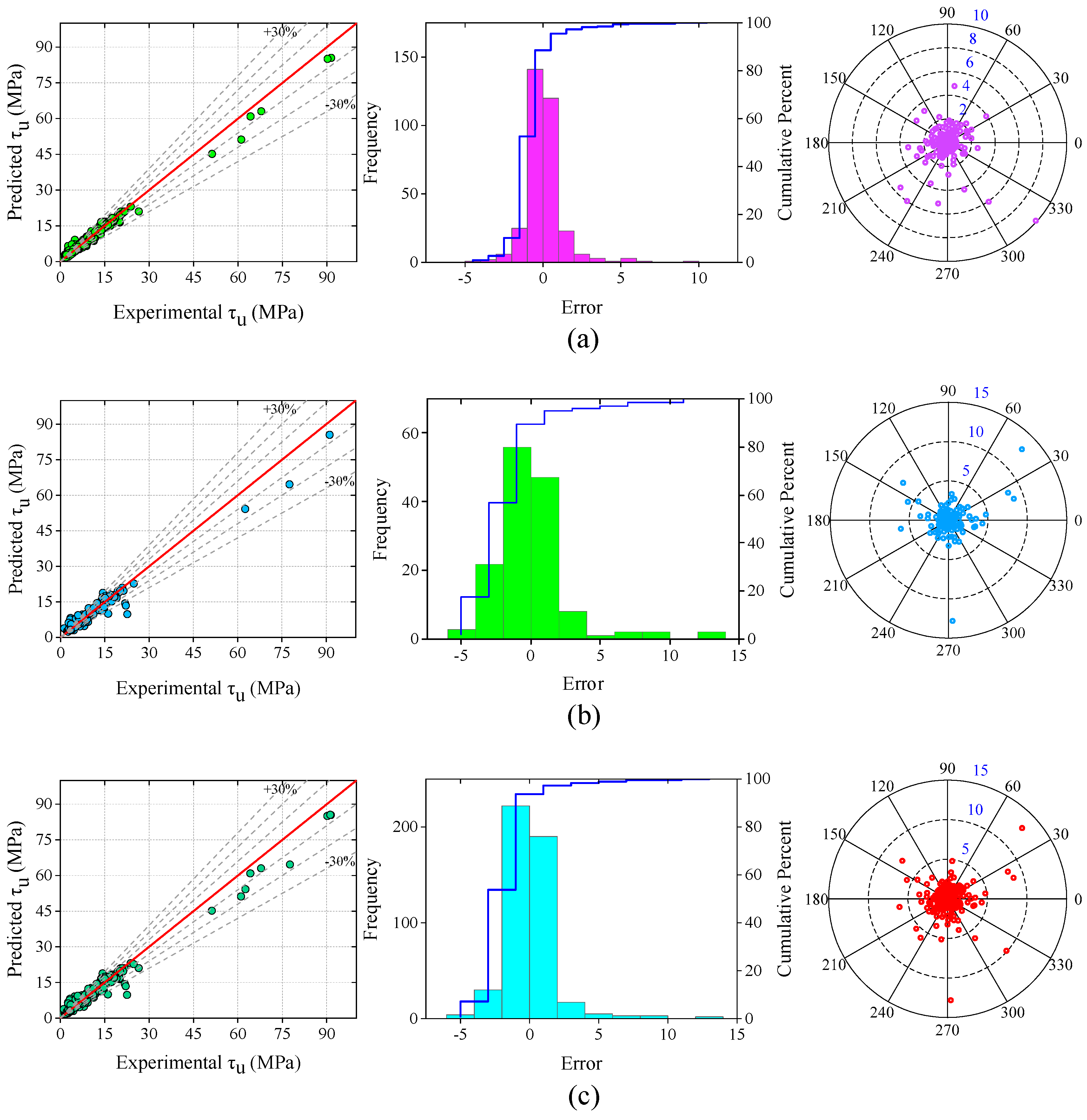
- The R-value of the ANN model was 0.99, which was 171.98% higher than the R-value of Model-10. The values of other performance metrics such as MAE, RMSE, MAPE, NS, and a20-index were 1.091 MPa, 1.495 MPa, 17.879%, 0.980, and 0.761, respectively. The values of MAE, MAPE, and RMSE of the ANN model were smaller than the error performance indices of Model-10. In addition, the NS and a20-index of the SVM and ANN models had higher values than Model-10 values.
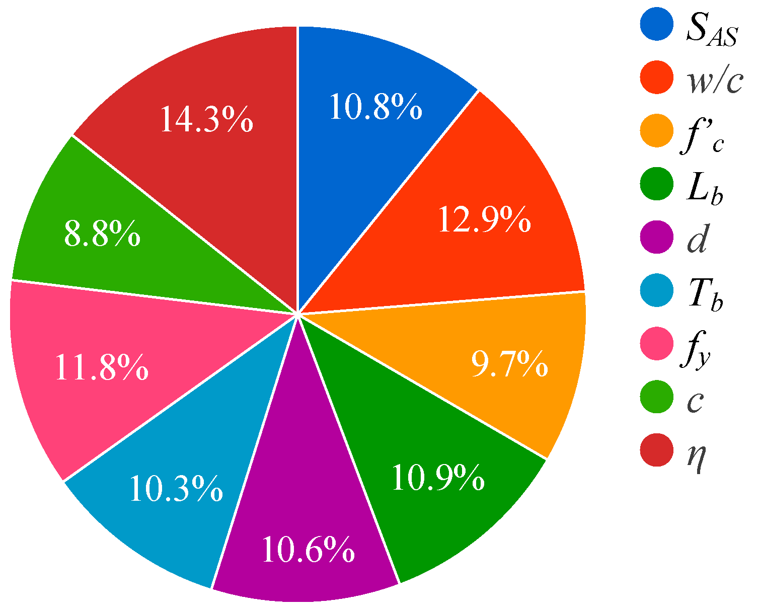
- Sensitivity analysis revealed that, as compared with other parameters, the corrosion level had the greatest influence on BS.
- Based on all the analyzed results as well as a graphical representation, it can be concluded that the performance of the ANN model was good, and the developed ML-based ANN model could effectively be used to predict BS of concrete to steel.
Author Contributions
Funding
Data Availability Statement
Conflicts of Interest
Nomenclature
| SVM | support vector machine | SAS | surface area of specimen |
| MLR | multiple linear regression | w/c | water/cement ratio |
| ANN | artificial neural network | f ′c | compressive strength |
| GEP | gene expression programming | Lb | bond length |
| RBFNN | radial basis function neural network | d | diameter of reinforcement bar |
| MLP | multilayer perceptron | Tb | type of reinforcement bar |
| LSSVR | least squares support vector regression | fy | yield strength of reinforcement bar |
| DFP | differential flower pollination | c | concrete cover |
| SVR | support vector regression | η | corrosion level |
| MGGP | multi-gene genetic programming | τu | bond strength |
| GA | genetic algorithm | PF | pullout force |
| FL | fuzzy logic | zn | normalized output of variable |
| ML | machine learning | z | variable of input to be normalized |
| ReLU | rectified linear unit | zmin | minimum value of input variable z |
| ANFIS | adaptive neuro-fuzzy inference system | zmax | minimum value of input variable z |
| GMDH | group method of data handling | r | actual output |
| MARS | multivariate adaptive regression spline | s | projected output |
| MNLR | multiple nonlinear regression | N | number of points in data set |
| KSM | Kriging surrogate model | Ni | input parameter (sum of biases, weights, and normalized inputs) |
| BPANN | back propagation ANN | Xi | normalized input value |
| RegTree | regression tree | Wi(H-O) | value of weight from hidden to output layer |
| PSO | particle swarm optimization | Wi(I-H) | value of weight from input to hidden layer |
| LMA | Levenberg–Marquardt algorithm | B(H-O) | value of bias from hidden to output layer |
| RMSE | root mean square error | B(I-H) | value of bias from input to hidden layer |
| MAE | mean absolute error | f(I-H) | AF that is used from input to hidden layer |
| MAPE | mean absolute percentage error | f(H-O) | AF that is used from hidden to output layer |
| R | correlation coefficient | Rr | relative rib area |
| NS | Nash-Sutcliffe efficiency index | Av/S | amount of transverse steel area to spacing ratio |
| RC | reinforced concrete | ls | splice length |
| Std. | standard deviation | ρ | splice bar size |
| MSE | mean square error | c/d | ratio of concrete cover to reinforcement bar diameter |
| BS | bond strength | Lb/d | ratio of bond length to reinforcement bar diameter |
| AF | activation function | Surf | reinforcement bar surface treatment |
| Ns | number of stirrups | Pos | reinforcement bar position/location |
| As | area of stirrups | Surf/Tr | ratio of reinforcement bar surface to transverse reinforcement bar |
| Cm | curing method | √f ′c | square root of concrete compressive strength |
| UHPC | ultra-high-performance concrete | Ad | anchorage depth |
| Atr | area of transverse reinforcement bar | Sd | surface dimensions of specimen |
| Ec | elastic modulus of concrete | Cs | crack severity of concrete |
| UPV | ultrasonic pulse velocity | Es/EFRP | ratio of elasticity modulus of steel reinforcement bars to that of FRP bars |
| ft | tensile strength of reinforcement bar | IEPSO | improved eliminate particle swarm optimization |
| St | surface treatment | IEPANN | improved eliminate particle swarm optimization hybridized ANN |
| i | interface moisture condition | PANN | particle swarm optimization hybridized ANN |
| Ct | type of concrete | Atr/Snd | ratio of area of transverse reinforcement bar to product (transverse bar spacing, number of developed bars, and bar diameter) |
References
- Kumar, A.; Arora, H.C.; Mohammed, M.A.; Kumar, K.; Nedoma, J. An Optimized Neuro-Bee Algorithm Approach to Predict the FRP-Concrete Bond Strength of RC Beams. IEEE Access 2022, 10, 3790–3806. [Google Scholar] [CrossRef]
- Bertolini, L. Steel corrosion and service life of reinforced concrete structures. Struct. Infrastruct. Eng. 2008, 4, 123–137. [Google Scholar] [CrossRef]
- Chung, L.; Cho, S.-H.; Kim, J.-H.J.; Yi, S.-T. Correction factor suggestion for ACI development length provisions based on flexural testing of RC slabs with various levels of corroded reinforcing bars. Eng. Struct. 2004, 26, 1013–1026. [Google Scholar] [CrossRef]
- Fu, B.; Chen, S.-Z.; Liu, X.-R.; Feng, D.-C. A probabilistic bond strength model for corroded reinforced concrete based on weighted averaging of non-fine-tuned machine learning models. Constr. Build. Mater. 2022, 318, 125767. [Google Scholar] [CrossRef]
- Bilek, V.; Bonczková, S.; Hurta, J.; Pytlík, D.; Mrovec, M. Bond Strength Between Reinforcing Steel and Different Types of Concrete. Procedia Eng. 2017, 190, 243–247. [Google Scholar] [CrossRef]
- Dauji, S.; Bhargava, K. Neural Estimation of Bond Strength Degradation in Concrete Affected by Reinforcement Corrosion. INAE Lett. 2018, 3, 203–215. [Google Scholar] [CrossRef]
- Mousavi, S.M.; Bahr Peyma, A.; Mousavi, S.R.; Moodi, Y. Predicting the Ultimate and Relative Bond Strength of Corroded Bars and Surrounding Concrete by Considering the Effect of Transverse Rebar Using Machine Learning. Iran. J. Sci. Technol. Trans. Civ. Eng. 2022, 1–27. [Google Scholar] [CrossRef]
- Coccia, S.; Imperatore, S.; Rinaldi, Z. Influence of corrosion on the bond strength of steel rebars in concrete. Mater. Struct. 2016, 49, 537–551. [Google Scholar] [CrossRef]
- Yalciner, H.; Eren, O.; Sensoy, S. An experimental study on the bond strength between reinforcement bars and concrete as a function of concrete cover, strength and corrosion level. Cem. Concr. Res. 2012, 42, 643–655. [Google Scholar] [CrossRef]
- Chung, L.; Kim, J.-H.J.; Yi, S.-T. Bond strength prediction for reinforced concrete members with highly corroded reinforcing bars. Cem. Concr. Compos. 2008, 30, 603–611. [Google Scholar] [CrossRef]
- Ma, Y.; Guo, Z.; Wang, L.; Zhang, J. Experimental investigation of corrosion effect on bond behavior between reinforcing bar and concrete. Constr. Build. Mater. 2017, 152, 240–249. [Google Scholar] [CrossRef]
- Choi, Y.S.; Yi, S.-T.; Kim, M.Y.; Jung, W.Y.; Yang, E.I. Effect of corrosion method of the reinforcing bar on bond characteristics in reinforced concrete specimens. Constr. Build. Mater. 2014, 54, 180–189. [Google Scholar] [CrossRef]
- Güneyisi, E.M.; Mermerdaş, K.; Gültekin, A. Evaluation and modeling of ultimate bond strength of corroded reinforcement in reinforced concrete elements. Mater. Struct. 2015, 49, 3195–3215. [Google Scholar] [CrossRef]
- Kapoor, N.R.; Kumar, A.; Arora, H.C.; Kumar, A. Structural Health Monitoring of Existing Building Structures for Creating Green Smart Cities Using Deep Learning. In Recurrent Neural Networks; CRC Press: Boca Raton, FL, USA, 2022; pp. 203–232. [Google Scholar] [CrossRef]
- Kumar, A.; Mor, N. An Approach-Driven: Use of Artificial Intelligence and Its Applications in Civil Engineering. Stud. Big Data 2021, 85, 201–221. [Google Scholar] [CrossRef]
- Kapoor, N.R.; Kumar, A.; Alam, T.; Kumar, A.; Kulkarni, K.S.; Blecich, P. A Review on Indoor Environment Quality of Indian School Classrooms. Sustainability 2021, 13, 11855. [Google Scholar] [CrossRef]
- Concha, N.C.; Oreta, A.W.C. Investigation of the effects of corrosion on bond strength of steel in concrete using neural network. Comput. Concr. 2021, 28, 77–91. [Google Scholar] [CrossRef]
- Rahman, S.; Al-Ameri, R. Experimental Investigation and Artificial Neural Network Based Prediction of Bond Strength in Self-Compacting Geopolymer Concrete Reinforced with Basalt FRP Bars. Appl. Sci. 2021, 11, 4889. [Google Scholar] [CrossRef]
- Farouk, A.I.B.; Zhu, J.; Ding, J.; Haruna, S. Prediction and uncertainty quantification of ultimate bond strength between UHPC and reinforcing steel bar using a hybrid machine learning approach. Constr. Build. Mater. 2022, 345, 128360. [Google Scholar] [CrossRef]
- Alizadeh, F.; Naderpour, H.; Mirrashid, M. Bond strength prediction of the composite rebars in concrete using innovative bio-inspired models. Eng. Rep. 2020, 2, e12260. [Google Scholar] [CrossRef]
- Amin, M.N.; Iqbal, M.; Salami, B.A.; Jamal, A.; Khan, K.; Abu-Arab, A.M.; Al-Ahmad, Q.M.S.; Imran, M. Predicting Bond Strength between FRP Rebars and Concrete by Deploying Gene Expression Programming Model. Polymers 2022, 14, 2145. [Google Scholar] [CrossRef]
- Ben Seghier, M.E.A.; Ouaer, H.; Ghriga, M.A.; Menad, N.A.; Thai, D.-K. Hybrid soft computational approaches for modeling the maximum ultimate bond strength between the corroded steel reinforcement and surrounding concrete. Neural Comput. Appl. 2020, 33, 6905–6920. [Google Scholar] [CrossRef]
- Yartsev, V.P.; Nikolyukin, A.N.; Pluzhnikova, T.M. Assessment and Modeling of Bond Strength of Corroded Reinforcement in Concrete Structures. Adv. Mater. Technol. 2018, 3, 070–082. [Google Scholar] [CrossRef]
- Bseiso, A.F. Development of Artificial Neural Network Software and Models for Engineering Materials. Available online: https://engagedscholarship.csuohio.edu/etdarchive/1259 (accessed on 23 October 2022).
- Kumar, A.; Arora, H.C.; Kumar, K.; Mohammed, M.A.; Majumdar, A.; Khamaksorn, A.; Thinnukool, O. Prediction of FRCM–Concrete Bond Strength with Machine Learning Approach. Sustainability 2022, 14, 845. [Google Scholar] [CrossRef]
- Golafshani, E.M.; Rahai, A.; Sebt, M.H.; Akbarpour, H. Prediction of bond strength of spliced steel bars in concrete using artificial neural network and fuzzy logic. Constr. Build. Mater. 2012, 36, 411–418. [Google Scholar] [CrossRef]
- Yan, F.; Lin, Z.; Wang, X.; Azarmi, F.; Sobolev, K. Evaluation and prediction of bond strength of GFRP-bar reinforced concrete using artificial neural network optimized with genetic algorithm. Compos. Struct. 2017, 161, 441–452. [Google Scholar] [CrossRef]
- Concha, N.C.; Oreta, A.W.C. Bond Strength Prediction Model of Corroded Reinforcement in Concrete Using Neural Network. Int. J. Geomate 2019, 16, 55–61. [Google Scholar] [CrossRef]
- Yartsev, V.P.; Nikolyukin, A.N.; Korneeva, A.O. Neural network modeling of concrete bond strength to reinforcement. IOP Conf. Series Mater. Sci. Eng. 2019, 687, 033011. [Google Scholar] [CrossRef]
- Bolandi, H.; Banzhaf, W.; Lajnef, N.; Barri, K.; Alavi, A.H. An Intelligent Model for the Prediction of Bond Strength of FRP Bars in Concrete: A Soft Computing Approach. Technologies 2019, 7, 42. [Google Scholar] [CrossRef] [Green Version]
- Hoang, N.-D.; Tran, X.-L.; Nguyen, H. Predicting ultimate bond strength of corroded reinforcement and surrounding concrete using a metaheuristic optimized least squares support vector regression model. Neural Comput. Appl. 2019, 32, 7289–7309. [Google Scholar] [CrossRef]
- Concha, N.; Oreta, A.W.C. An Improved Prediction Model for Bond Strength of Deformed Bars in RC Using UPV Test and Artificial Neural Network. Int. J. Geomate 2020, 18, 179–184. [Google Scholar] [CrossRef]
- Shahri, S.F.; Mousavi, S.R. Bond strength prediction of spliced GFRP bars in concrete beams using soft computing methods. Comput. Concr. 2021, 27, 305–317. [Google Scholar]
- Farouk, A.I.B.; Jinsong, Z. Prediction of Interface Bond Strength Between Ultra-High-Performance Concrete (UHPC) and Normal Strength Concrete (NSC) Using a Machine Learning Approach. Arab. J. Sci. Eng. 2022, 47, 5337–5363. [Google Scholar] [CrossRef]
- Wei-liang, J.; Yu-xi, Z. Effect of corrosion on bond behavior and bending strength of reinforced concrete beams. J. Zhejiang Univ. Sci. A 2001, 2, 298–308. [Google Scholar]
- Horrigmoe, G.; Saether, I.; Antonsen, R.; Arntsen, B. Laboratory Investigations of Steel Bar Corrosion in Concrete: Sustainable Bridges Background Document SB3.10. Available online: http://ltu.diva-portal.org/smash/record.jsf?pid=diva2%3A1337406&dswid=7939 (accessed on 23 October 2022).
- Zhao, Y.; Lin, H.; Wu, K.; Jin, W. Bond behaviour of normal/recycled concrete and corroded steel bars. Constr. Build. Mater. 2013, 48, 348–359. [Google Scholar] [CrossRef]
- Yalciner, H.; Marar, K. Experimental Study on the Bond Strength of Different Geometries of Corroded and Uncorroded Reinforcement Bars. J. Mater. Civ. Eng. 2017, 29, 1–10. [Google Scholar] [CrossRef]
- Hou, L.; Liu, H.; Xu, S.; Zhuang, N.; Chen, D. Effect of corrosion on bond behaviors of rebar embedded in ultra-high toughness cementitious composite. Constr. Build. Mater. 2017, 138, 141–150. [Google Scholar] [CrossRef]
- Mak, M.W.T.; Desnerck, P.; Lees, J.M. Corrosion-induced cracking and bond strength in reinforced concrete. Constr. Build. Mater. 2019, 208, 228–241. [Google Scholar] [CrossRef]
- Tariq, F.; Bhargava, P. Bond characteristics of corroded pullout specimens exposed to elevated temperatures. Structures 2020, 25, 311–322. [Google Scholar] [CrossRef]
- Vuong, D.D.T.; Hung, N.T.; Hung, N.D. Experimental study on the effect of concrete strength and corrosion level on bond between steel bar and concrete. Transp. Commun. Sci. J. 2021, 72, 498–509. [Google Scholar] [CrossRef]
- Lu, Z.-H.; Wu, S.-Y.; Tang, Z.; Zhao, Y.-G.; Li, W. Effect of chloride-induced corrosion on the bond behaviors between steel strands and concrete. Mater. Struct. 2021, 54, 129. [Google Scholar] [CrossRef]
- Kumar, A.; Arora, H.C.; Kapoor, N.R.; Mohammed, M.A.; Kumar, K.; Majumdar, A.; Thinnukool, O. Compressive Strength Prediction of Lightweight Concrete: Machine Learning Models. Sustainability 2022, 14, 2404. [Google Scholar] [CrossRef]
- Kapoor, N.R.; Kumar, A.; Kumar, A.; Kumar, A.; Mohammed, M.A.; Kumar, K.; Kadry, S.; Lim, S. Machine Learning-Based CO2 Prediction for Office Room: A Pilot Study. Wirel. Commun. Mob. Comput. 2022, 2022, 9404807. [Google Scholar] [CrossRef]
- Kapoor, N.R.; Kumar, A.; Kumar, A. Machine Learning Algorithms for Predicting Viral Transmission Probability in Naturally Ventilated Office Rooms. In Proceedings of the Paper Presented at the 2nd International Conference on i-Converge 2022: Changing Dimensions of the Built Environment, Dehradun, India, 15–17 September 2022. [Google Scholar]
- Kumar, A.; Arora, H.C.; Kapoor, N.R.; Kumar, K. Prognosis of compressive strength of fly-ash-based geopolymer-modified sustainable concrete with ML algorithms. Struct. Concr. 2022. [Google Scholar] [CrossRef]
- Kumar, K.; Saini, R. Adaptive neuro-fuzzy interface system based performance monitoring technique for hydropower plants. ISH J. Hydraul. Eng. 2022, 1–11. [Google Scholar] [CrossRef]
- Cabrera, J. Deterioration of concrete due to reinforcement steel corrosion. Cem. Concr. Compos. 1996, 18, 47–59. [Google Scholar] [CrossRef]
- Lee, H.-S.; Noguchi, T.; Tomosawa, F. Evaluation of the bond properties between concrete and reinforcement as a function of the degree of reinforcement corrosion. Cem. Concr. Res. 2002, 32, 1313–1318. [Google Scholar] [CrossRef]
- Stanish, K.; Hooton, R.D.; Pantazopoulou, S.J. Corrosion effects on bond strength in reinforced concrete. ACI Struct. J. 1999, 96, 915–921. [Google Scholar]
- Aslani, F.; Nejadi, S. Bond Behavior of Reinforcement in Conventional and Self-Compacting Concrete. Adv. Struct. Eng. 2012, 15, 2033–2051. [Google Scholar] [CrossRef]
- Australian Standard, A.S. 3600; Concrete Structures. 3Concrete Structures. Standards Australia: Sydney, Australia, 2004.
- Orangun, C.O.; Jirsa, J.O.; Breen, J.E. The Strength of Anchored Bars: A Reevaluation of Test Data on Development Length and Splices; Center for Highway Research, University of Texas at Austin: Austin, TX, USA, 1975. [Google Scholar]
- Orangun, C.O.; Jirsa, J.O.; Breen, J.E. A Reevaluation of Test Data on Development Length and Splices. ACI J. Proc. 1977, 74, 114–122. [Google Scholar]
- Esfahani, M.R.; Rangan, B.V. Bond between Normal Strength and High-Strength Concrete (HSC) and Reinforcing Bars in Splices in Beams. ACI Struct. J. 1998, 95, 272–279. [Google Scholar]
- Comite Euro-International Du Beton. CEB-FIP Model Code 1990: Design Code; Thomas Telford Publishing: London, UK, 1993; pp. 33–81. [Google Scholar] [CrossRef]
- Wang, X.; Liu, Y.; Xin, H. Bond strength prediction of concrete-encased steel structures using hybrid machine learning method. Structures 2021, 32, 2279–2292. [Google Scholar] [CrossRef]
- Diab, A.M.; Elyamany, H.E.; Hussein, M.A.; Al Ashy, H.M. Bond behavior and assessment of design ultimate bond stress of normal and high strength concrete. Alex. Eng. J. 2014, 53, 355–371. [Google Scholar] [CrossRef] [Green Version]
- Eligehausen, R.; Popov, E.P.; Bertero, V.V. Local bond stress-slip relationships of deformed bars under generalized excitations. Athens Techn. Chamb. Greece 1982, 4, 69–80. [Google Scholar] [CrossRef]
- Amini Pishro, A.; Feng, X.; Ping, Y.; Dengshi, H.; Shirazinejad, R.S. Comprehensive equation of local bond stress between UHPC and reinforcing steel bars. Constr. Build. Mater. 2020, 262, 119942. [Google Scholar] [CrossRef]
- Su, M.; Zhong, Q.; Peng, H.; Li, S. Selected machine learning approaches for predicting the interfacial bond strength between FRPs and concrete. Constr. Build. Mater. 2020, 270, 121456. [Google Scholar] [CrossRef]
- Da Silva, I.N.; Hernane Spatti, D.; Andrade Flauzino, R.; Liboni, L.H.B.; dos Reis Alves, S.F. Artificial Neural Networks; Springer: Cham, Switzerland, 2017. [Google Scholar]
- Afandi, A.; Lusi, N.; Catrawedarma, I.; Subono; Rudiyanto, B. Prediction of temperature in 2 meters temperature probe survey in Blawan geothermal field using artificial neural network (ANN) method. Case Stud. Therm. Eng. 2022, 38, 102309. [Google Scholar] [CrossRef]
- Ahmadi, M.; Kheyroddin, A.; Kioumarsi, M. Prediction models for bond strength of steel reinforcement with consideration of corrosion. Mater. Today Proc. 2021, 45, 5829–5834. [Google Scholar] [CrossRef]


| S. No. | References | Input Parameter | AI Method Used | Bond Range (MPa) | R (Best Method Value) |
|---|---|---|---|---|---|
| 1 | Golafshani et al. [26] | f ′c, c, Av/S, Rr, ρ, ls | ANN, FL | 1.521–8.994 | 0.993 (FL) |
| 2 | Güneyisi et al. [13] | f ′c, c, Tb, d, Lb, η | GEP, ANN | 1.3–31.7 | 0.96 (ANN) |
| 3 | Yan et al. [27] | d, c/d, Lb/d, d, Surf, Pos, Surf/Tr, √f ′c | ANN, GA | 2.4–24.52 | 0.945 (ANN-GA) |
| 4 | Yartsev et al. [23] | f ′c, d, η, Ad, Sd, Surf | ANN | 1.3–31.7 | 0.94721 (ANN) |
| 5 | Concha and Oreta [28] | f ′c, Lb, d, c, UPV, η, ft, Cs | ANN | Average = 6.591 | 0.957 (ANN) |
| 6 | Yartsev et al. [29] | f ′c, ft, Ad, Surf, Tb, Ec | ANN | — | 0.947 (ANN) |
| 7 | Bolandi et al. [30] | Surf, Pos, d, c/d, Lb/d, f ′c | MGGP | 0.76–21 | 0.961 (MGGP) |
| 8 | Hoang et al. [31] | f ′c, c, Tb, d, Lb, η | LSSVR, DFP | 1.3–31.7 | 0.9505 (DFP-LSSVR) |
| 9 | Alizadeh et al. [20] | Surf, Pos, d, c/d, Lb/d, f ′c, Atr/Snd | ANFIS, ANN, GMDH | 1.64–22.34 | 0.988 (ANFIS) |
| 10 | Concha and Oreta [32] | f ′c, ft, Lb, d, c, UPV | ANN | Std. deviation = 6.376 | 0.981 (ANN) |
| 11 | Bseiso [24] | η, c, f ′c | ANN-ReLU, ANN-S | 1.3–31.7 | 0.983 (ANN-ReLU) |
| 12 | Ben Seghier et al. [22] | f ′c, c, Tb, d, Lb, η | MLP, RBFNN, GEP | 1.3–31.7 | 0.97 (MLP-LMA) |
| 13 | Concha and Oreta [17] | f ′c, Lb, c/d, UPV | ANN | 6.029–30.922 | 0.927 (ANN) |
| 14 | Shahri and Mousavi [33] | f ′c, d, Surf, Lb/d, c/d, Es/EFRP, Atr/Snd | M5 model tree, MARS, KSM | 1.06–6.73 | 0.969 (MARS) |
| 15 | Rahman and Al-Ameri [18] | f ′c, c/d, Lb/d, Lb, d, Ct | ANN | 2.32–14.15 | 0.963 (ANN) |
| 16 | Farouk and Jinsong [34] | f ′c, UHPC, Cm, St, Im | SVM, MLR, ANN | 0.5–8.85; 1.19–41.2 | 0.979 (SVM) (Splitting); 0.925 (SVM) (Slant shear) |
| 17 | Mousavi et al. [7] | f ′c, c, d, Lb, fy, Ns, As, η | MLP, ANN, RBFNN, SVR | 0.19–91.42 | 0.977 (SVR) |
| 18 | Amin et al. [21] | d, f ′c, c/d, Lb/d | GEP | 0.76–21 | 0.963 (GEP) |
| 19 | Farouk et al. [19] | d, f ′c, fy, d, Lb, c | MLR, SVM, PANN, IEPANN | 11.1–71.79 | 0.973 (IEPANN) |
| S. No. | References | No. of Specimens | Input Parameters | Output | ||||||||
|---|---|---|---|---|---|---|---|---|---|---|---|---|
| SAS (mm2) | w/c | f ′c (MPa) | Lb (mm) | d (mm) | Tb | fy (MPa) | c (mm) | η (%) | τu (MPa) | |||
| 1 | Wei-Liang and Yu-xi [35] | 27 | 10,000 | 0.55 | 22.13 | 80 | 12 | 1–2 | 389–428 | 44 | 0.12–9.99 | 1.4–11.34 |
| 2 | Horrigmoe et al. [36] | 32 | 80,424.77 | 0.68 | 30 | 160 | 25 | 2 | 500 | 147.5 | 0–6.82 | 3.89–11.91 |
| 3 | Chung et al. [10] | 40 | 30,000 | 0.58 | 28.3 | 39 | 13 | 2 | 526.8 | 68.5 | 0–8.8 | 9.4–20.1 |
| 4 | Yalciner et al. [9] | 57 | 22,500 | 0.4–0.75 | 23–51 | 50 | 14 | 2 | 458 | 15–45 | 0–18.75 | 1.8–21.7 |
| 5 | Zhao et al. [37] | 11 | 22,500 | 0.36 | 38.4–41.9 | 100 | 18 | 2 | 357.5 | 66 | 0–6.18 | 1.18–6.39 |
| 6 | Choi et al. [12] | 9 | 22,500 | 0.4–0.6 | 21–32 | 100 | 25 | 2 | 524 | 62.5 | 0–9.98 | 51.23–91.42 |
| 7 | Coccia et al. [8] | 10 | 22,500 | 0.7 | 29 | 70 | 12 | 2 | 507.5 | 69 | 0–3.92 | 4.7–14.13 |
| 8 | Ma et al. [11] | 33 | 22,500 | 0.48 | 24.81 | 100 | 18–22 | 1–2 | 258.68–373.64 | 30 | 0–10.41 | 1.83–9.05 |
| 9 | Yalciner and Marar [38] | 156 | 40,000 | 0.63–0.79 | 24–38 | 220–270 | 14 | 4 | 459 | 30–45 | 0–4.3 | 2.134–9.167 |
| 10 | Hou et al. [39] | 42 | 22,500 | 0.45 | 45.5 | 48–112 | 16 | 2 | 456 | 48.07–50.27 | 0–15.25 | 10.05–21.28 |
| 11 | Mak et al. [40] | 9 | 8992.02 | 0.6 | 22.8–30.7 | 50 | 10 | 2 | 530 | 48.5 | 0–22.9 | 10.1–17.9 |
| 12 | Tariq and Bhargava [41] | 37 | 5026.55–31,415.93 | 0.4 | 35 | 40–100 | 8–20 | 2 | 550 | 36–90 | 0–16 | 0.19–22.59 |
| 13 | Vuong et al. [42] | 12 | 40,000 | 0.38–0.48 | 24.6–44.1 | 60 | 12 | 2 | 400 | 94 | 0–12.93 | 13.81–26.51 |
| 14 | Lu et al. [43] | 1 | 14,400 | 0.42 | 52.6 | 80 | 15.2 | 3 | 1828 | 52.4 | 0 | 11.2 |
| Parameter | Symbol Used | Unit | Minimum | Maximum | Mean | Std. |
|---|---|---|---|---|---|---|
| Concrete | SAS | mm2 | 5026.55 | 80,424.77 | 31,715.84 | 16,660.00 |
| w/c | _ | 0.36 | 0.79 | 0.59 | 0.14 | |
| f ′c | MPa | 21.00 | 52.60 | 31.78 | 8.36 | |
| c | mm | 15.00 | 147.50 | 52.39 | 30.82 | |
| Lb | mm | 39.00 | 270.00 | 132.17 | 84.75 | |
| Reinforcement Bar | d | mm | 8.00 | 25.00 | 15.23 | 3.83 |
| Tb | _ | 1.00 | 4.00 | 2.59 | 1.01 | |
| fy | MPa | 258.68 | 1828.00 | 463.93 | 86.39 | |
| η | % | 0.00 | 22.90 | 3.41 | 4.05 | |
| BS | τu | MPa | 0.19 | 91.42 | 10.01 | 10.60 |
| Model | References | Formulation | Remarks |
|---|---|---|---|
| Model-1 | Cabrera [49] | = BS (MPa), C = Corrosion level (%) | |
| Model-2 | Lee et al. [50] | = BS (MPa), = Corrosion percentage (%), = CS (MPa) | |
| Model-3 | Stanish et al. [51] | = BS (MPa), = Corrosion percentage (%), = CS (MPa) | |
| Model-4 | Chung et al. [10] | = BS (MPa), = Corrosion percentage (%) | |
| Model-5 | Aslani and Nejadi [52] | For plain bars, For deformed bars, | = BS (MPa), c = Concrete cover (mm), = Diameter of bars (mm), = Bond length (mm), = CS (MPa) |
| Model-6 | Yalciner et al. [9] | For uncorroded specimens, For corroded specimens, (R2 = 0.98) | = BS (MPa), c = Concrete cover (mm), D = Diameter of bars (mm), = CS (MPa), = Corrosion level (%) |
| Model-7 | Yalciner and Marar [38] | For uncorroded specimens, For corroded specimens, | c = Concrete cover (mm), D = Diameter of bars (mm), = CS (MPa), = BS (MPa), = Corrosion level (%) |
| Model-8 | Yalciner and Marar [38] | For uncorroded specimens, For corroded specimens, | = BS (MPa), = Concrete cover (mm), = Diameter of bars (mm), = Corrosion level (%), = CS (MPa) |
| Model-9 | Australian Standard 3600 [53] | — | |
| Model-10 | Orangun et al. [54,55] | — | |
| Model-11 | Esfahani and Rangan [56] | — | |
| Model-12 | CEB-FIP [57] | = BS (MPa), = CS (MPa) | |
| Model-13 | CEB-FIP [57] | — | |
| Model-14 | Hou et al. [39] | = BS (MPa), = Diameter of bars (mm), = Bond length (mm), = Corrosion ratio (%) | |
| Model-15 | Wang et al. [58] | = CS (MPa) | |
| Model-16 | Wang et al. [58] | — | |
| Model-17 | Diab et al. [59] | — | |
| Model-18 | Eligehausen et al. [60] | — | |
| Model-19 | Amini Pishro et al. [61] | — | |
| Model-20 | CEB-FIP [57] | = BS (MPa), = CS (MPa) |
| S. No. | Group | Model | R | MAE (MPa) | MAPE (%) | RMSE (MPa) | a20-Index | NS |
|---|---|---|---|---|---|---|---|---|
| 1 | Group-I | Model-6 | 0.053 | 9.580 | 241.660 | 13.203 | 0.141 | −0.161 |
| 2 | Model-7 | 0.054 | 7.954 | 209.657 | 12.480 | 0.212 | −0.289 | |
| 3 | Model-8 | 0.069 | 6.503 | 137.778 | 11.300 | 0.191 | −0.133 | |
| 4 | Model-4 | 0.101 | 7.982 | 147.153 | 11.545 | 0.183 | −0.054 | |
| 5 | Model-1 | 0.107 | 12.036 | 222.142 | 14.462 | 0.103 | −0.084 | |
| 6 | Model-16 | 0.126 | 9.008 | 83.371 | 13.891 | 0.006 | 0.001 | |
| 7 | Model-12 | 0.138 | 7.650 | 174.141 | 11.218 | 0.183 | 0.016 | |
| 8 | Model-15 | 0.138 | 7.872 | 69.634 | 13.088 | 0.040 | 0.009 | |
| 9 | Model-20 | 0.138 | 7.550 | 170.961 | 11.149 | 0.181 | 0.016 | |
| 10 | Model-13 | 0.139 | 6.128 | 59.549 | 11.777 | 0.179 | 0.003 | |
| 11 | Model-2 | 0.146 | 5.788 | 58.224 | 11.158 | 0.185 | −0.007 | |
| 12 | Group-II | Model-9 | 0.160 | 5.550 | 65.313 | 11.275 | 0.223 | 0.019 |
| 13 | Model-19 | 0.168 | 20.017 | 422.526 | 21.771 | 0.017 | −0.075 | |
| 14 | Model-3 | 0.171 | 6.477 | 50.691 | 12.192 | 0.191 | 0.014 | |
| 15 | Model-11 | 0.171 | 5.964 | 125.361 | 10.549 | 0.189 | 0.020 | |
| 16 | Model-18 | 0.174 | 5.254 | 77.912 | 10.705 | 0.229 | 0.029 | |
| 17 | Model-17 | 0.298 | 6.582 | 89.402 | 11.639 | 0.151 | −0.130 | |
| 18 | Group-III | Model-5 | 0.363 | 5.984 | 139.444 | 10.432 | 0.288 | 0.112 |
| 19 | Model-10 | 0.364 | 4.514 | 87.517 | 9.888 | 0.275 | 0.131 | |
| 20 | Model-14 | 0.397 | 7.794 | 181.843 | 11.132 | 0.187 | 0.123 |
| Model | R | MAE (MPa) | MAPE (%) | RMSE (MPa) | a20-Index | NS |
|---|---|---|---|---|---|---|
| ANN-Training | 0.994 | 0.844 | 13.669 | 1.127 | 0.834 | 0.987 |
| ANN-Validation | 0.948 | 1.213 | 16.855 | 1.681 | 0.667 | 0.896 |
| ANN-Testing | 0.995 | 1.319 | 19.235 | 1.665 | 0.625 | 0.990 |
| ANN-All | 0.990 | 1.091 | 17.879 | 1.495 | 0.761 | 0.980 |
| SVM-Training | 0.993 | 0.896 | 15.799 | 1.336 | 0.826 | 0.983 |
| SVM-Testing | 0.979 | 1.642 | 22.937 | 2.608 | 0.693 | 0.948 |
| SVM-All | 0.989 | 1.120 | 18.438 | 1.814 | 0.786 | 0.971 |
| Group | Model | R | MAE (MPa) | MAPE (%) | RMSE (MPa) | NS | a20-Index |
|---|---|---|---|---|---|---|---|
| Group-I | Model-2 | 0.146 | 5.788 | 58.224 | 11.158 | −0.007 | 0.185 |
| Group-II | Model-18 | 0.174 | 5.254 | 77.912 | 10.705 | 0.029 | 0.229 |
| Group-III | Model-10 | 0.364 | 4.514 | 87.517 | 9.888 | 0.131 | 0.275 |
| Existing model | Mousavi et al. [7] | 0.977 | - | - | 5.372 | - | - |
| Proposed model-I | SVM | 0.989 | 1.120 | 18.438 | 1.814 | 0.971 | 0.786 |
| Proposed model-II | ANN | 0.990 | 1.091 | 17.879 | 1.495 | 0.980 | 0.761 |
Publisher’s Note: MDPI stays neutral with regard to jurisdictional claims in published maps and institutional affiliations. |
© 2022 by the authors. Licensee MDPI, Basel, Switzerland. This article is an open access article distributed under the terms and conditions of the Creative Commons Attribution (CC BY) license (https://creativecommons.org/licenses/by/4.0/).
Share and Cite
Singh, R.; Arora, H.C.; Bahrami, A.; Kumar, A.; Kapoor, N.R.; Kumar, K.; Rai, H.S. Enhancing Sustainability of Corroded RC Structures: Estimating Steel-to-Concrete Bond Strength with ANN and SVM Algorithms. Materials 2022, 15, 8295. https://doi.org/10.3390/ma15238295
Singh R, Arora HC, Bahrami A, Kumar A, Kapoor NR, Kumar K, Rai HS. Enhancing Sustainability of Corroded RC Structures: Estimating Steel-to-Concrete Bond Strength with ANN and SVM Algorithms. Materials. 2022; 15(23):8295. https://doi.org/10.3390/ma15238295
Chicago/Turabian StyleSingh, Rohan, Harish Chandra Arora, Alireza Bahrami, Aman Kumar, Nishant Raj Kapoor, Krishna Kumar, and Hardeep Singh Rai. 2022. "Enhancing Sustainability of Corroded RC Structures: Estimating Steel-to-Concrete Bond Strength with ANN and SVM Algorithms" Materials 15, no. 23: 8295. https://doi.org/10.3390/ma15238295