1. Introduction
Recently, global energy policy has been increasingly oriented towards the exploitation of renewable energy sources (RESs) to reduce carbon dioxide emissions (mainly responsible for the reduction of the ozone layer in the atmosphere, which protects the earth from the harmful action of UV rays) [
1,
2,
3]. In this framework, microgrids (MGs), smaller local electricity networks that can also be operated individually, have established themselves as solutions for managing energy flows from RESs for future smart networks [
4,
5,
6]. MGs, depending on the operating mode, can be divided into direct current (DC-MG) [
7,
8,
9] and alternative current (AC-MG) microgrids. Compared to the AC-MGs, the DC-MGs, which also operate in isolated mode, provide better performance regarding the management of energy flows coming from RESs (photovoltaic (PV), wind (WT), fuel cell (FC) [
10]) with storage systems [
11] towards electrical loads both civil and industrial without the need for DC/AC converters for the integrated system and without requiring synchronization operations [
12,
13,
14].
Recent works of scientific literature propose efficient algorithms for the control and management of energy flow, ensuring maximum power transfer (through the use of maximum point power (MPPT) directly in the algorithms [
15,
16]), even in adverse or otherwise changing weather conditions [
17,
18,
19,
20]. However, it should be noted that the scale limitations and the limited capacity of the accumulator do not allow AC-MGs to provide long-term energy, so it is necessary to use modular FCs to guarantee adequate power with continuity and with rapid response to load variations (common diesel generators are to be excluded because they are polluting and characterized by reduced efficiency) [
21,
22]. Stationary FCs stand out among them as they can be used in contexts where the quantity of energy required is significant [
23,
24,
25].
Obviously, the energy management system (EMS) is the core of an MG which should be able, on the one hand, to standardize the power exchanged between RESs and loads (in compliance with the respective constraints) and, on the other, to reduce costs and increase the lifetime of the MG [
26,
27,
28].
Furthermore, EMSs, in case of interruption of the primary power supply, should be able to start the backup power supply by starting the FC which, coupled to an electrolyzer, produces the fuel (for example, hydrogen (
)) on demand [
29,
30,
31].
Now, many authors are busily engaged in the design and validation of EMSs for DC-MGs with high reliability and performance. There is no lack of theoretical studies of physical-mathematical modeling of MGs with certainly interesting results, but almost all are based on the resolution of systems of differential equations [
32,
33]. However, it is worth noting that the systems of differential equations that describe the dynamic behaviors of PV and WT powers have different operating times and therefore suffer from synchronization problems [
34,
35,
36,
37]. A possible solution would require the adaptive insertion of delay times into each of the equations, resulting in the challenge of obtaining numerical solutions within a reasonable time. It follows that the mathematical models for this MG are currently not very efficient [
38,
39,
40].
Recently, a considerable number of works have been produced reporting interesting DC-MG studies which also propose sophisticated topologies with latest-generation energy storage and production elements [
41,
42,
43] equipped with multi-level hierarchical control systems to optimize any fuel consumption [
44,
45].
With the widespread diffusion of approaches based on artificial intelligence (AI), scientific production in the DC-MG field has recently achieved important results thanks to the strong peculiarity of these techniques in the processing of large quantities of data for the process of decision making. In fact, machine learning techniques have opened wide frontiers, especially in the study of stability (regression [
26,
46,
47], random forest tree [
26,
48,
49], convolutional neural networks [
26,
50,
51] and others [
52,
53,
54]). However, these techniques, although promising in performance and results obtained, have the flaw of being black-box type procedures so, on the one hand, they are difficult to understand by non-experts and, on the other, they do not allow updates except in the case of substantial interventions.
In AI, soft computing comes into play and, in particular, fuzzy systems (FSs) which represent flexible evolutionary models that solve non-linear problems (difficult to solve using equations and/or mathematical algorithms) where human intelligence is required [
55]. FSs, by formulating “
...
” banks of fuzzy rules, solve problems in which the data used are affected by uncertainties and/or inaccuracies [
56,
57,
58]. With the help of these techniques, numerous EMSs have been designed and tested for DC-MGs with PV and WT power generation with the integration of a battery storage and FC with the aim of reducing costs by maximizing power. However, even if the results appear valuable, in some cases the naive approach makes performance inefficient [
26,
59,
60]. Obviously, there is no shortage of significant advances regarding the fuzzy EMS control procedure of DC-MGs, based on automatic extraction of the fuzzy rule bank [
61,
62,
63], fault detection and classification [
64,
65,
66].
However, to consider any uncertainties in writing the membership functions, only recently have significant works been produced on the management and control of EMSs in DC-MGs using fuzzy systems based on intuitionistic fuzzy sets without, however, considering any need to adaptively optimize the fuzzy membership functions (FMFs) [
67,
68,
69]. To our knowledge, until now no significant work has been published regarding this important task for the DC-MGs of the future.
With this objective in mind (i.e., reducing
consumption to a minimum and maximizing the power of the RESs), we start with the DC-MG in island mode (
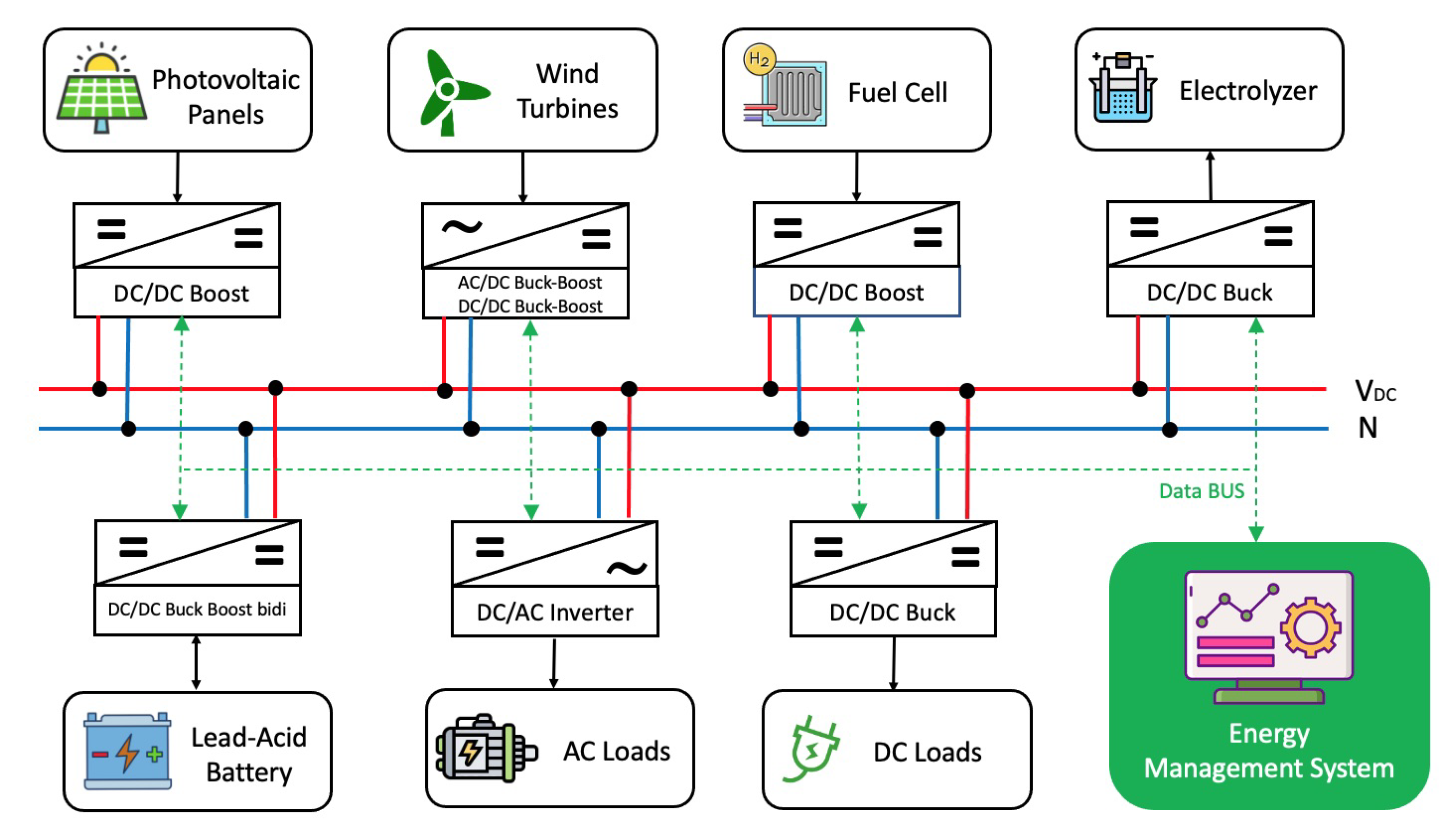
Figure 1) proposed in [
26] which, through a Mamdani fuzzy EMS, managed the power supply of domestic users with RESs (PV/WT) and a lead-acid storage system supported by a
cell in which the inputs were the net power and state of charge (SoC) of the battery and the output was the power of the
cell. As detailed in
Figure 1, the system is composed of a load connected to the RESs via electronic converters acting as a connection between the system devices and the backup system (lead-acid battery and
production/consumption). Furthermore, each subsystem is accompanied by a local control device (based on decentralized architecture) and an EMS characterized by centralized supervision.
Even if the results in [
26] were noteworthy (since they reduced hydrogen consumption by increasing the power extractable from the RESs), no adaptive procedure was recognized regarding the writing of the fuzzy rules (in particular, of the FMFs) which, in that case, were built through experience gained over the years by the authors without any optimized tuning process.
Therefore, starting from the aforementioned EMS, in this work, to consider any uncertainties in the membership values, we rewrite the bank of fuzzy rules according to an innovative optimized intuitionistic Takagi–Sugeno (TS) approach exploiting a procedure based on the subtractive cluster technique able to optimize the FMFs.
The main contributions of this paper are summarized in the following list.
The fuzzy (heuristic) Mamdani model proposed in [
26], although it does not require a mathematical model to structure the EMS allowing for easy upgradeability, does not provide a detailed description of the process. It also does not allow the use of design techniques in the form of rules with optimization of the shape and position of the membership functions for each variable involved. Finally, Mamdani’s approach, which has limited validity to the data intervals used for its definition, does not allow guidelines for the definition of the model’s characteristics (i.e., order, number and form of qualifiers, number and content of the rules).
Since the problem under study has two inputs and one output (MISO), the fuzzy model studied in [
26] was rewritten according to the TS approach. This fuzzy approach, regarding the fuzzification and application of connectives, maintains the same steps as the Mamdani inference. Furthermore, the output is structured as a set of singletons which, appropriately combined, provide functional (deterministic) consequences.
It can be immediately observed that the fuzzy rules presented in [
26] arise from the expert’s knowledge, which is essentially derived from the behavior of the individual elements that constitute the MG. The behavior of many of them (unfortunately not all) is described deterministically by a system of evolutionary differential equations whose solutions provide indications to the expert for the composition of the fuzzy rules. However, to reduce the risk of fuzzy rule banks with numerous rules, and at the same time start evaluating any fuzzy assumptions for stability, it appears necessary to verify that these evolutionary models admit a single solution (thus ensuring that, at least in principle, the outputs of fuzzy systems do not represent ghost solutions [
70,
71]). So, in this article, before proceeding with the design of fuzzy systems, this verification was performed using analytical techniques now consolidated in the literature.
The main reason why it was chosen to transform the Mamdani model studied in [
26] concerns the great potential that TS models have in the clustering of the antecedents (to determine the number of rules) and in the structuring of the consequent (which culminates in functional deterministic expression of the output), as well as providing banks of fuzzy rules and inferences that are completely general and not limited to a few inputs and rules. Particularly, to structure the antecedents of each rule, an AI heuristic iterative technique based on particle swarm optimization (PSO) was exploited, as required by the specifications of the Tech4You Project. The proposed approach can identify “optimum candidates” in the search space based on specific quality measures. Even if the most recent scientific literature proposes innovative alternative techniques for the intended objective, the PSO, by not making any assumptions on the problem, allows the exploration of considerable solution spaces. Furthermore, by not using differential operators during the optimization process, differentiability of the issue under study is not required, opening up broad prospects of success for that entire class of irregular, noisy concerns with uncertainties and/or inaccuracies.
As regards the structuring of the consequent, an approach based on batch least squares (BLS) was used which, in synergy with the PSO, determines the optimal allocation of the output singletons with a limited computational complexity.
While obtaining promising results following the use of the EMS managed by the optimized fuzzy TS, it is appropriate to consider any additional uncertainties contained in each membership function involved in each fuzzy rule. With this objective in mind, the optimized TS fuzzy model was generalized considering both membership and non-membership values, inducing the formulation of a respective degree of hesitation. The proposed procedure allowed us to build a fuzzy TS (intuitionistic) system which, through clustering of the antecedents, also determines the number of rules (with a high performance estimated using an appropriate index).
The three EMSs obtained (managed by the aforementioned fuzzy systems) were tested in an area located in southern Italy (38
7
15.138
N/15
39
55.315
E) in correspondence with the buildings of the DICEAM Departments of the “Mediterranea” University of Reggio Calabria (Italy) now involved in the activities of the aforementioned Project (Tech4You Spoke 2 Project—Goal 2.1—PP1—Action 9). The results obtained, in maximizing the power provided by the RESs and reducing the production of
, are fully comparable with the performances obtained through the TS type formulation of the model in [
26] optimized using the combined particle swarm approach optimization (PSO) and batch least squares (BLS), but with better performance results and CPU-time, which is interesting for any real-time applications and technological transfer as well.
The remainder of the paper is structured as follows. After briefly describing the configuration of the DG-MG studied in [
26] (
Section 2), the physical-mathematical characteristics of the RESs used are detailed, highlighting that the evolutionary differential models for managing the exchange of information with the DC bus are well posed (
Section 3). Next,
Section 4 details the peculiar characteristics of the starting EMS that uses the Mamdani approach, including the bank of fuzzy rules that manages the control. Then,
Section 5 details the steps that allow the formulation of the optimized TS approach, while
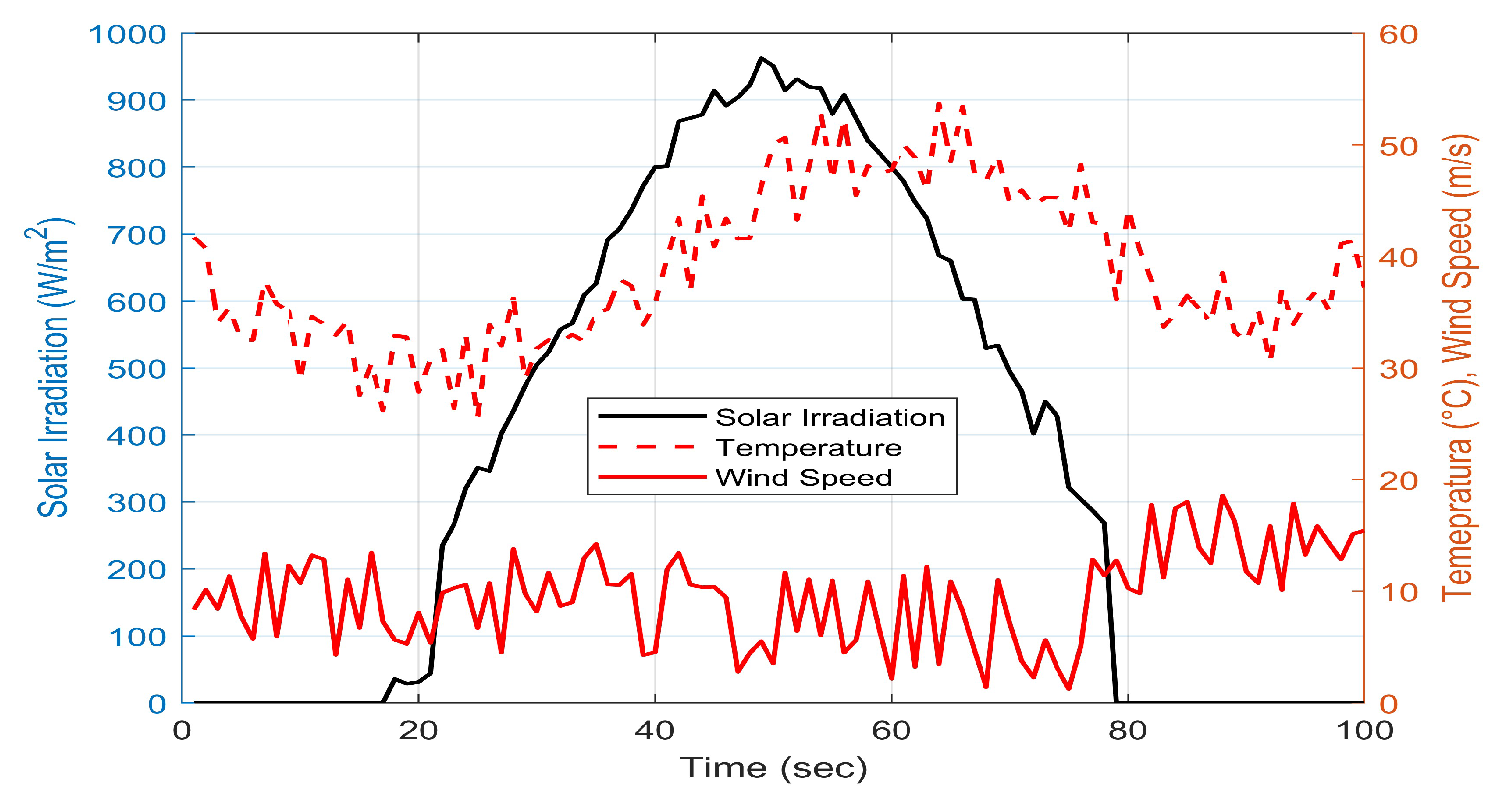
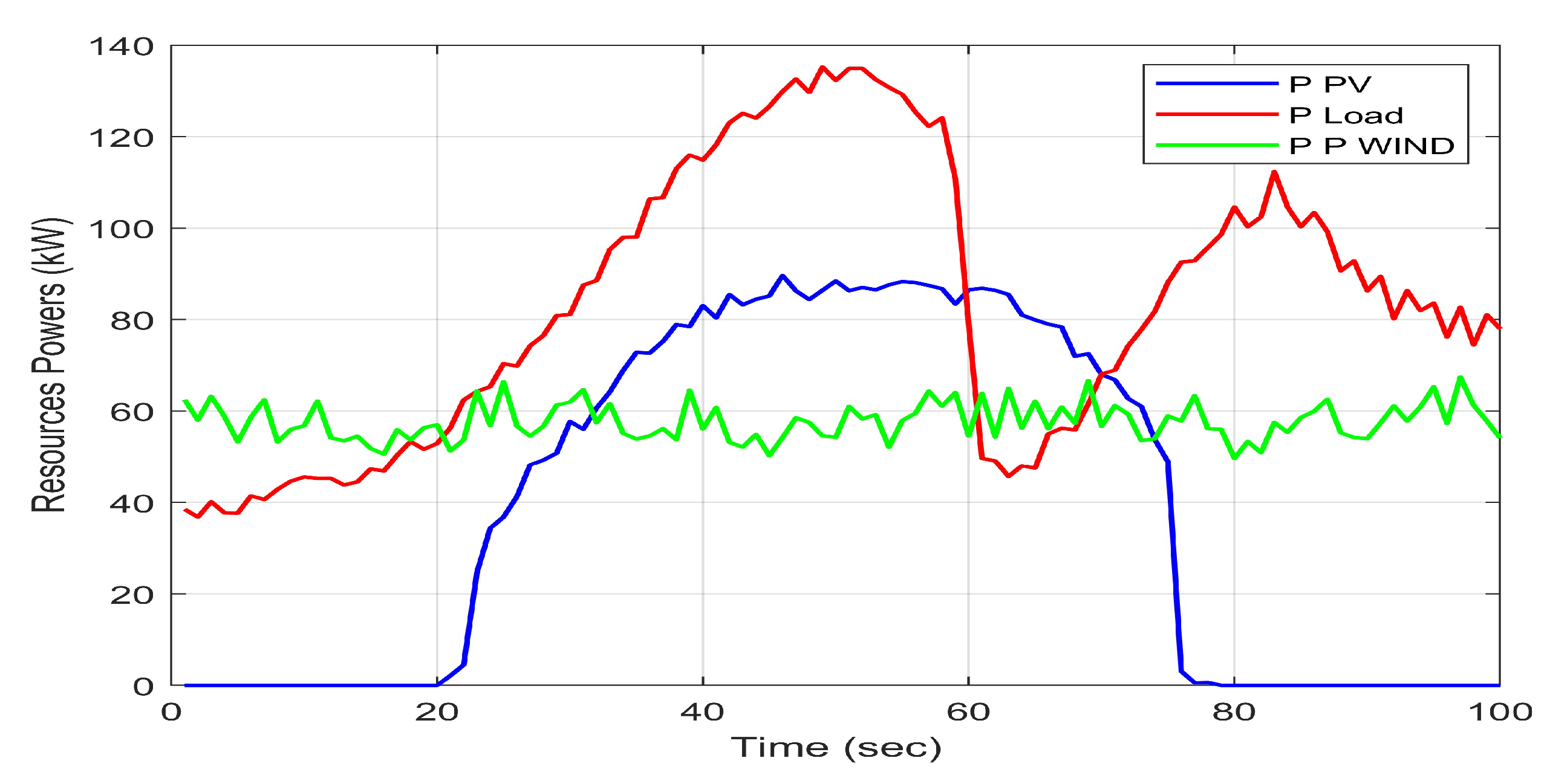
Section 6 describes the structure of the optimized fuzzy system which exploits the intuitionistic approach. Once the electrical loads have been described by outlining the meteorological parameters and power profiles of the RESs considered as reported in
Section 7, the implementation aspects are highlighted in
Section 8 introducing the initial relevant results.
Section 9 is dedicated to discussing the performance while the conclusions and possible future perspectives conclude the paper. As a summary of the entire work, an appendix contains the proofs of the theorems that establish the well-posedness of each evolutionary differential model.
2. DC-MG Structure: An Overview
As can be seen from
Figure 1, the starting DC-MG considered in this paper, as in [
26], is made up of two primary renewable sources, PV and WT, operating in MPTT mode generating 100 kW and 50 kW, respectively. Furthermore, a
FC functions as a secondary source and guarantees, if necessary, enough energy (50 kW at nominal state, 60 kW at maximum power) to avoid blackout situations. And again, a 50 kW battery stabilizes the voltage on the DC bus, providing energy to the grid if necessary and absorbing any excess energy, while a dump-load electrolyzer (DC charge) absorbs excess energy if the generated power exceeds that of the load with an SoC over
. Finally, some DC and AC domestic loads complete the MG. In particular, as regards the wind turbine, a double AC/DC and DC/DC converter has been inserted in a single block so that the second converter acts as an interface with the DC bus. Furthermore, the electrolyzer has been positioned to interact with the fuel cell allowing the DC-powered electrolyzer to produce hydrogen during the accumulation phase by storing it in tanks. The fuel cell converts the hydrogen back into electrical energy in DC during peak absorption. As regards the connection lines, in
Figure 1, the power flows have been indicated by arrows. In particular, the red/blue lines indicate the DC bus, while the green dotted line indicates the data bus to monitor the operation of the DC-MG (power flows, voltages, currents⋯). Finally, the black lines indicate the power flows of the various elements. As is known [
26], the power balance equation for the aforementioned MG is the following:
Furthermore, 50 kW represents the maximum charge/discharge power of the battery; when it is discharged, the energy comes from the RESs. In any case, it will absorb extra energy until the SoC reaches 80%, using the surplus energy to produce
in an electrolyzer.
Table 1 lists the complete parameters of the DC-MG as reported in [
26].
4. The Energy Management Systems: A Mamdani Fuzzy Approach
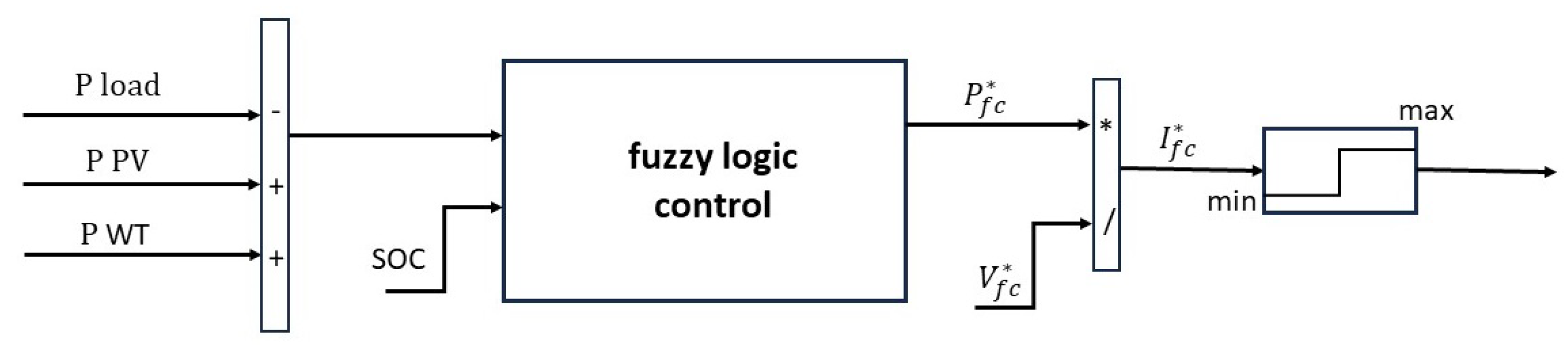
In this work, we start with the EMS based on a fuzzy Mamdani multi-input single-output (MISO) system studied in [
26], and structured through a rule bank based on the expert’s knowledge (considering any limitations and non-linear behaviors that each component highlighted). The system ensured a uniform power profile of the islanded DC-MG, reducing power fluctuations and peaks. As shown in
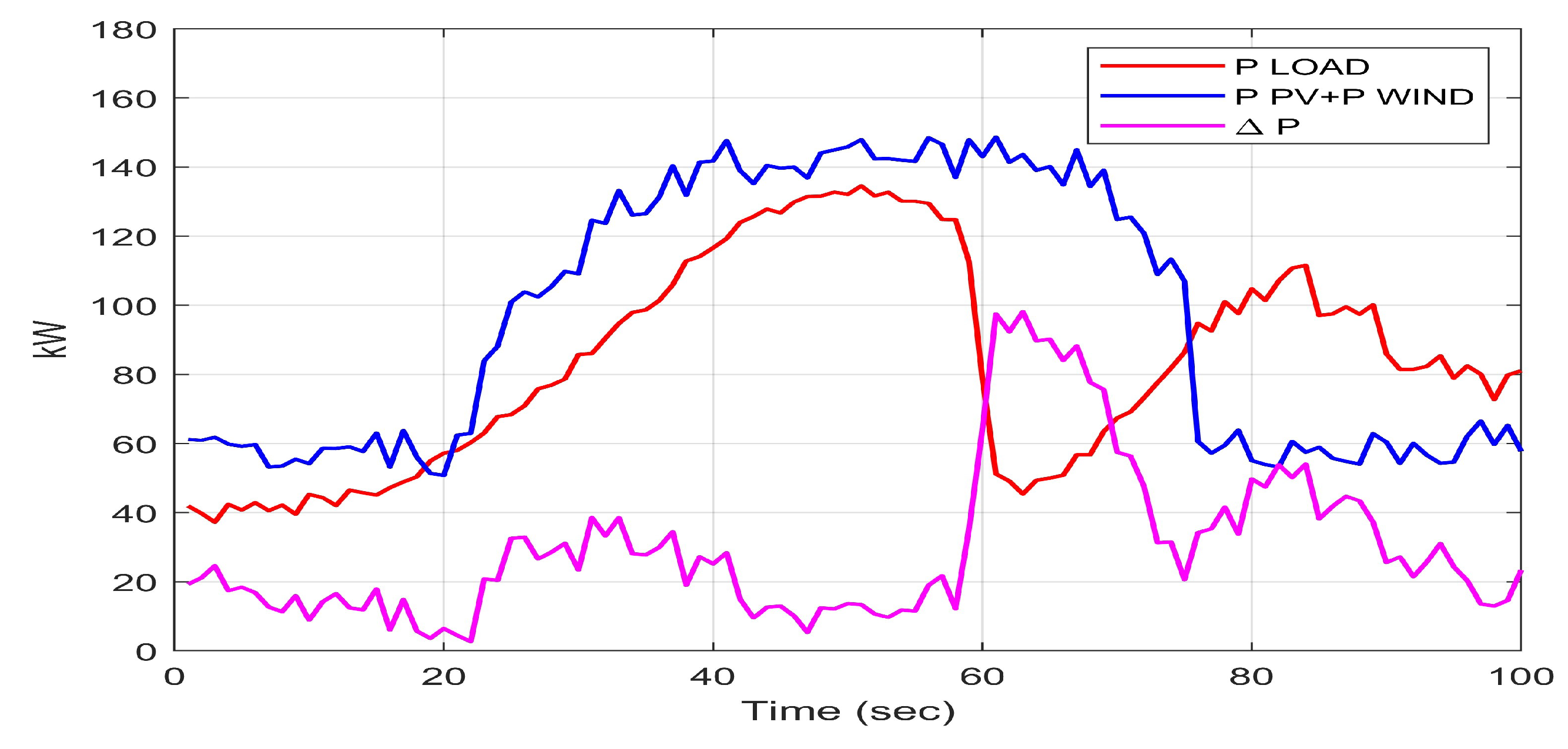
Figure 2, the system inputs are
, which subtracts the power of the renewable sources from the load power, and the SoC of the accumulator considering the reference power FC as production. The MISO fuzzy system depicted in
Figure 2 represents the EMS of the MG under study, whose MatLab/Simulink scheme is displayed in
Figure 3.
In particular, the FIS considered in [
26] treated
and
through linguistic subsets operating on the respective universes of discourse. The range of possible values for each variable (universe of discourse,
), as specified in [
26], are:
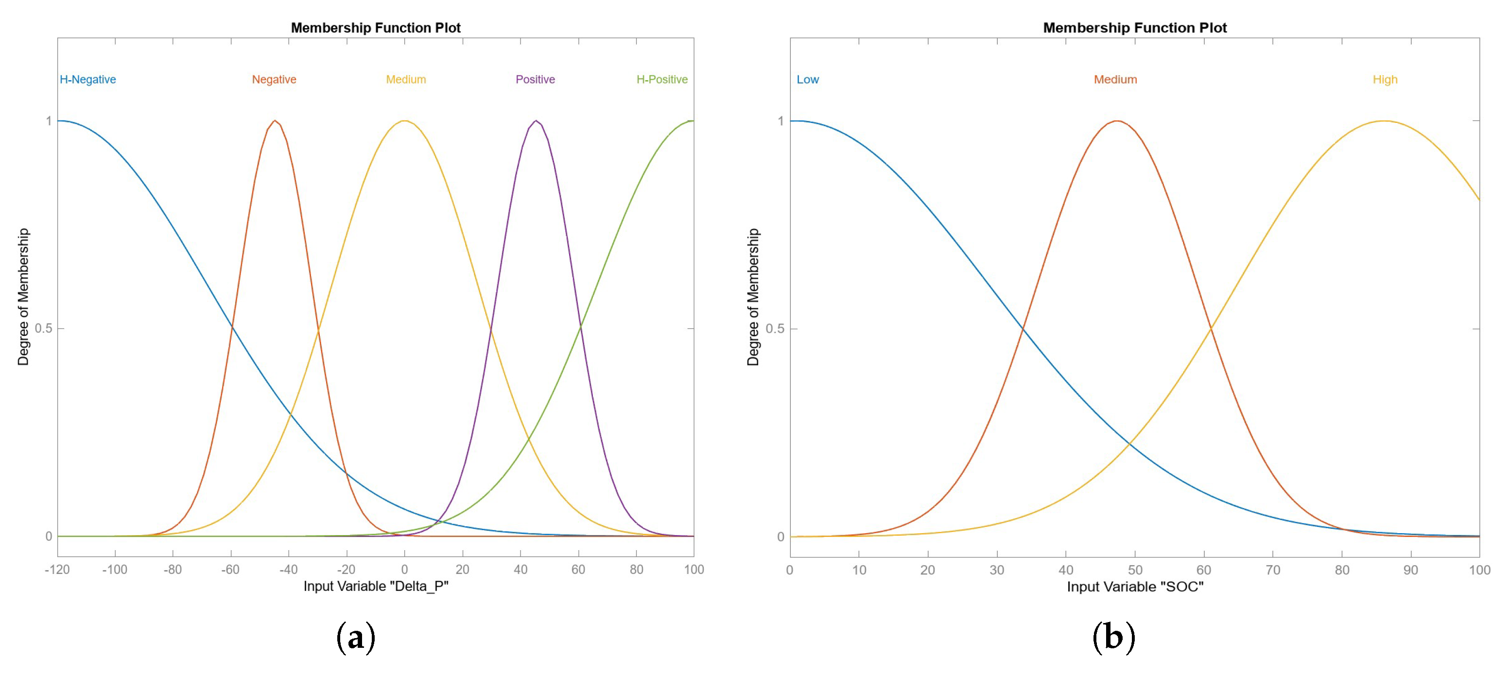
Moreover, for each variable, trapezoidal/triangular FMFs have been formulated to fuzzify each variable,
, as follows
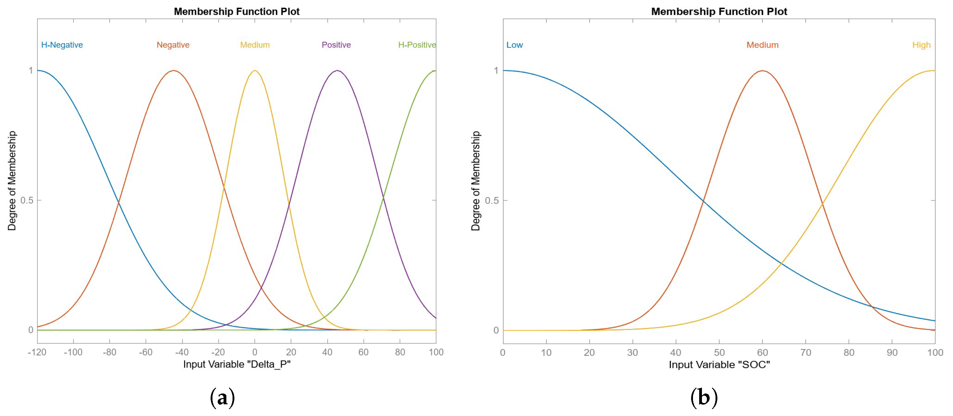
As detailed in
Table 2, for
, five FMFs were considered (High-Negative,
, Negative,
, Medium,
, Positive,
, High-Positive,
); for
, three MFs have been considered (Low,
, Medium,
, High,
); finally, for
four FMFs have been considered (Very-Low,
, Low,
, Medium,
, High,
).
The criterion with which the fuzzy rules were constructed (see
Table 3) is based on the following assumptions:
- (a)
If the has a low value and the has a strongly negative value, the is certainly high, so the FC should deliver maximum power while, if the has a negative value, the has a medium and therefore the cell would deliver half the power;
- (b)
In the case in which the has a low value and stands at average values, should be low so that the cell delivers reduced power, unlike the case where stands at positive (highly positive) values, requiring low (very low) values;
- (c)
The situation is a little more complex when stands at average values. In these cases, if is clearly negative (negative, highly positive), would settle at average values (low, very low) and therefore the cell would deliver an average value (low, very low, very low) of power;
- (d)
If has a high value and has a highly negative value (negative, positive, highly positive), has a medium value (medium, very low, very low); then, the FC delivers half (reduced percentage, reduced percentage) of the power that can be delivered.
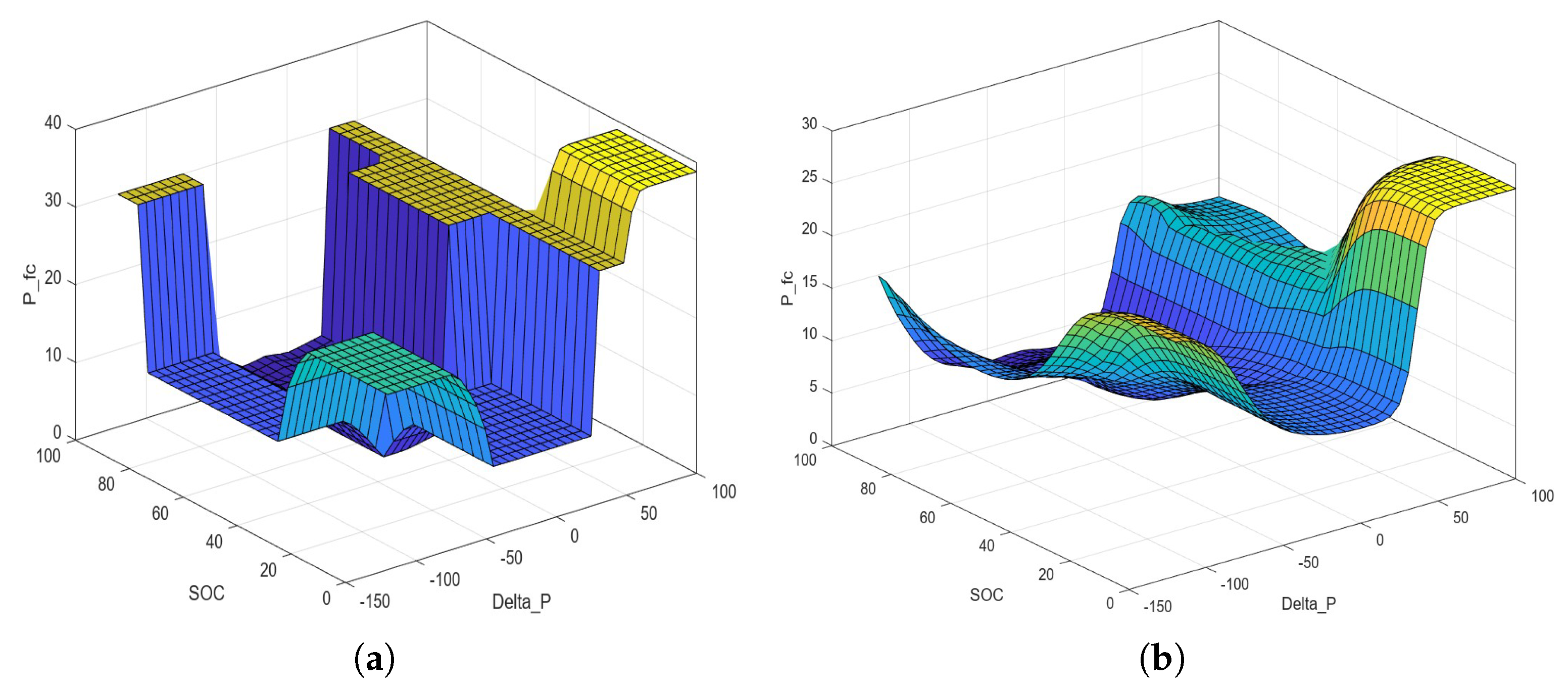
A fuzzy inference applies the rules to each input, obtaining a composite fuzzy set generated by the union of two or more MFs (depending on the number of activated rules) via a t-norm based on the evaluation of the minimum value of the membership degrees involved. Finally, the centroid was extracted from the aforementioned composite fuzzy set to obtain a crisp value of the output. However, it is worth noting that Mamdani-type FISs, even though they are characterized by precise fuzzifications and linguistically interpretable rules (hence adaptable to human input), provide less flexibility in the design of EMSs. This is because they provide moderately discontinuous surface output, requiring quantified .
5. The Energy Management System: A TS Optimized Approach
Fuzzy inference (or fuzzy reasoning) is used in a fuzzy rule to determine the result starting from the inputs. The fuzzy rules, as a whole, represent the control strategy starting from knowledge and/or experience. In each rule, the information assigned to the input variables (via the antecedent) is transferred to the consequent via fuzzy inference. To remedy the disadvantages of an EMS designed with the Mamdani approach, in this paper we reformulate the problem for TS inference, typical of MISO systems, where the antecedent parts of the fuzzy rules, regarding the Mamdani formulation, remain unchanged. As presented in [
26], a fuzzy Mamdani rule is made up of two fundamental sections: the first section, which precedes “THEN”, represents its antecedent while what follows “THEN” represents its consequent. After fuzzifying the data, the rule applies the fuzzy “and” operator (i.e., Mamdani minimum inference or drastic product inference) to the resulting operations on the membership values in the rule, obtaining a combined fuzzy membership value that is the result obtained from the antecedent of the same rule. Then, the “THEN” operator represents the inference of the rule as it transfers the information from the antecedent to the consequent. In particular, the Mamdani procedure cuts the output fuzzy set to the fuzzy membership value obtained by applying the “and” connective (i.e., the combined value obtained above) [
26]. Obviously, each rule provides its cut fuzzy set as explained above. These cut fuzzy sets are then aggregated together, usually through superposition and consequent envelope, whose center of gravity is the real number representing the defuzzified value of the output.
For TS fuzzy rules, while maintaining the same steps as Mamdani’s inference regarding fuzzification and connective application, the output is structured as a set of singletons and a typical fuzzy rule assumes the following form
in which the output is performed via linear polynomial combination of the inputs,
and
, even if higher-degree polynomials can be taken into account with significant increase in computational complexity. In (
23),
and
represent the FMFs, affected by the
k-th fuzzy rule, of the two inputs, respectively. Moreover,
and
indicate the model parameters to be trained. Then, for a generic fuzzy rule, we indicate by
and
the membership values of
to
and
to
, respectively, and since the “and” connective is present, the output will be activated at the value
. Therefore, the output,
y, is achieved by applying the generalized defuzzifier,
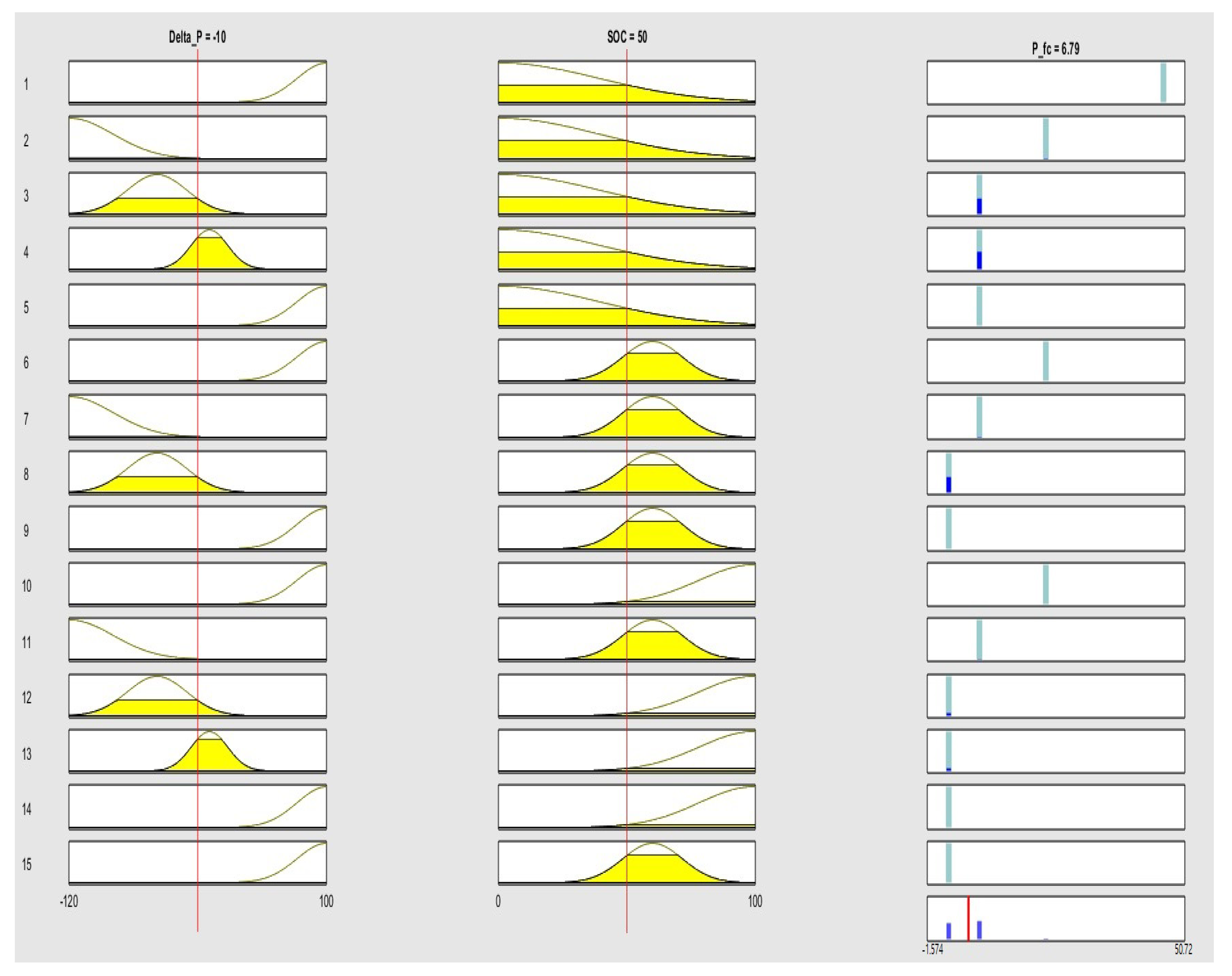
To better understand how (
24) works, consider as an example the fuzzy inference illustrated in
Figure 4 whose fuzzy rules are structured as in (
23). It is worth noting that not all fuzzy rules are always activated. For example, by choosing (at random)
and
as input variables, it is easy to verify that only some rules are activated (in this case, rules 3, 4, 8, 12 and 13 are activated). From
Figure 4, we can easily see that
activates the first rule with an activation degree
while
activates the first rule with an activation degree
. Since a fuzzy rule is stable when the output is activated with
[
72], it follows that the first fuzzy rule does not participate in the definition of the output.
Table 4 displays all the activation coefficients for each inference rule depicted in
Figure 4.
Therefore, according to
Table 4, (
24) becomes
in which the weights
and
are determined by the procedure described below.
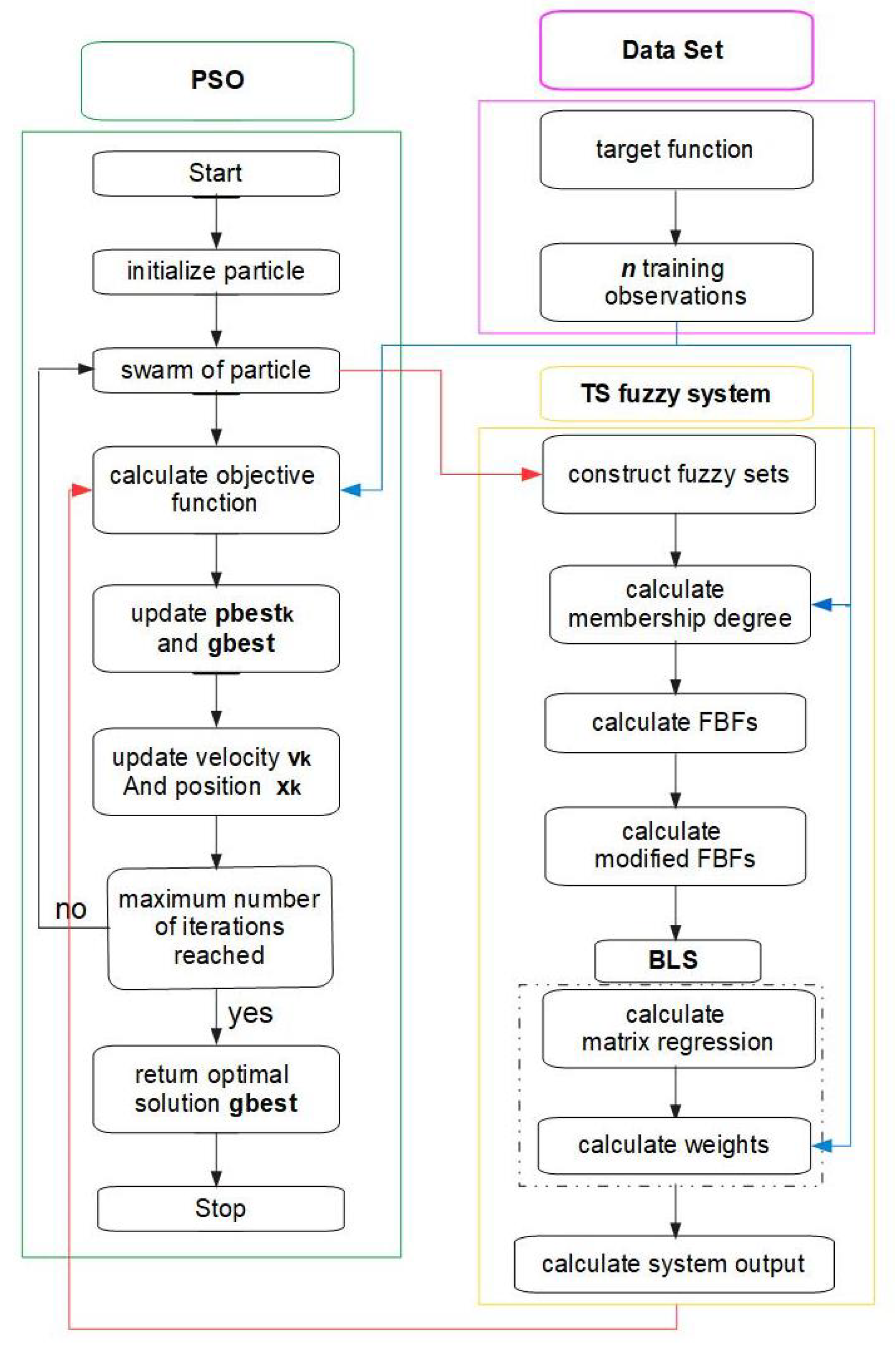
The system was trained using PSO to obtain the parameters of the fuzzy sets associated with the antecedents, while the BLS-based approach was exploited to obtain the polynomial coefficients of the output. In particular, in each iteration of the PSO procedure, each particle of the swarm contains the characteristic parameters of the Gaussian membership functions (peaks and widths) which, through the BLS approach, determine the consequent of the fuzzy rules. As the iterations proceed, the particles move in the definition space, generating a new set of parameters which will generate as many consequences. The best solution is obtained by minimizing an objective function.
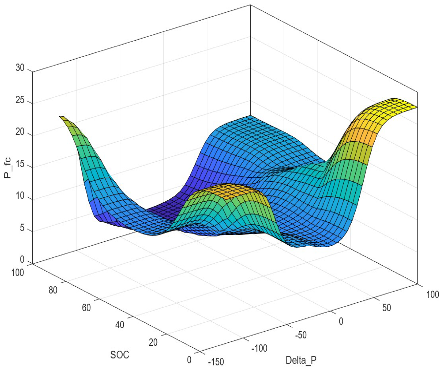
Such FSs have greater flexibility in design by obtaining continuous surface outputs. Finally, a tuning procedure has been exploited to optimize the localization for each FMF.
5.1. PSO for Structuring the Antecedents of Each Fuzzy Rule
PSO considers a group of particles dispersed in a given search space. Let
d be the dimension of this space. A generic particle, equipped with position,
, and velocity,
, with the best local position,
, accesses the best global position
, identified from the swarm, through the optimization of an objective function based on the PSO algorithm in which the velocity and position of the particles are calculated as follows [
74]:
in which
and
represent two vectors with uniformly distributed random numbers in
,
i is the current iteration number and
and
are positive constants. In (
26), the addends inertial considers the tendency of the particle to move in the same direction, the cognitive considers the attraction towards their best personal positions and the social considers possible movements towards the best positions previously found by any particle [
74].
5.2. BLS for Optimizing the Fuzzy Output
Indicating by [
74]
the fuzzy basic functions (FBFs), the output of the system can be written as follows,
Furthermore, setting (modified FBFs)
we finally achieve
Output (
31) can be written in matrix form. In fact, indicating by
we easily achieve:
in which
To obtain the model parameters, consider
n training observations,
,
, from which to construct the following regression model
We introduce the following cost function to minimize:
in which
is the output (
31), which represents a measure of precision to determine the accuracy of the model (the lower this value, the more accurate the performance).
Therefore, if
, the optimal solution is given by
in which
is the input data matrix. Obviously, if the problem is an ill-posed one, (
38) is rewritten in the following more convenient form
where
is a positive regularization parameter and, as usual,
is the identity matrix. Thus, for the cost function (
37), we need to add the addend
obtaining:
5.3. BLS and PSO: Steps of the Procedure
The approach we propose starts by setting both the maximum number of iterations, , and the number of particles.
Each particle represents a peak or the width of each Gaussian representing a fuzzy set. Thus, the particles for each rule are [
74]
Each particle is initialized by the following assumptions:
in which
and
with,
,
Furthermore, recent scientific literature suggests the following good position [
74]
The next step, starting from
and
,
and
, updates
and
by
respectively, in which “rand” is a randomly generated number belonging to
. Moreover,
and
represent the widths of the initialization ranges for the peaks. Furthermore,
and
with
.
Exploiting (
35),
,
are determined which contain the modified fuzzy basis functions as defined in (
30).
Next, the regression matrix (
36) is computed to then determine the polynomial coefficients (
38). Obviously, if
is a singular matrix, (
39) is used instead of (
38) (using an appropriate
), then calculating the RMSE,
For particles that exhibit repeating peaks, a penalty is applied by assigning them a high value of the objective function.
Next,
and
are updated based on the evaluation of the objective function. Therefore, by (
26) and (
27), both the velocity and the position are updated.
At this point, we limit the peaks and into the intervals, and ; just as and are limited in the intervals and .
Finally, the whole procedure repeats until the number of iterations reaches
. Then, the obtained
provides the best solution.
Figure 5 displays the flow diagram showing all the steps of the procedure.
6. The Energy Management System: A TS Intuitionistic Fuzzy Approach
An IF set is an object in
structured in the following form:
where
and
, such that
and
represent the membership and non-membership functions. Moreover, it is also defined as another function,
which represents the hesitation part (the larger
, the greater the decision maker’s margin of hesitation), increasing the accuracy in the management of uncertainties. Then, the need arises to construct two FISs: one relating to the function
, whose
k-th rule takes the form:
another, relative to the function
, where the
k-th rule becomes:
Each fuzzy rule produces two outputs,
and
, which, similarly to what was done in the TS approach (non-intuitionistic), can be written as follows
Finally, the convex combination of
and
produces the final output of the intuitionistic FIS:
in which
represents the weight of
.
Remark 9. Obviously, if , the system becomes a classical TS; if , only the non-membership component impacts the TS system. In this paper, to equally consider the components (membership and non-membership), we set .
As is known, Mamdani fuzzy systems build the fuzzy rule bank through manual inspection, resulting in a limitation to recognizing all the rules. To determine the number and antecedents of the fuzzy rules, we use a Subtractive Clustering Algorithm (SCA) so that the cluster centers determine N and the antecedents. In particular, the real data provided by the Technical Physics research group of the DICEAM Department has been structured into two technical sheets (one for inputs and one for output) made up of a single column and with an adequate number of rows for containing all the linguistic information associated with each input and the output (translated into ASCII format).
Next, it is necessary to set a constant positive that governs the spatial influence of the cluster,
: high values of
generate few fuzzy rules; small values of
could produce a high number of cluster centers producing the overfitting phenomenon. Then, the optimization of the parameters
,
, ⋯,
, and
,
, ⋯,
, with
in both (
59) and (
60) determine the consequent of each rule. In SCA, each data point is considered a potential cluster center. The extent of the potential of each point
, here, is quantified via the following formulation,
in which
and
represent two generic data points. Therefore, there will exist a data point, relative to many points close to it, that exhibits the maximum value of
; this data point represents the first cluster center,
.
Next, on this first cluster center, a new radius is fixed,
, which determines its neighborhood; thus, if
is the potential of
,
represents the quantity to subtract from
to obtain its updated value, that is,
becomes
The procedure is repeated until all the data points are associated with one or more clusters. Obviously, each
will be decomposed into two component vectors;
, which contains the first
n elements of
(i.e., input data), and
, which contains the output component. Since the intuitionistic system considered is first-order, it makes sense to compute the output as
where
is a constant vector and
is a real constant (even zero). To easily understand the approach for parameter estimation, it will be sufficient to interpret the procedure as the least squares estimate of the form
where
is an array of output values,
is a constant array and
is an array of parameters to estimate. To compute
, minimize
. Alternatively, it is possible by computing the pseudo-inverse of
, that is,
Since the calculation of
is quite onerous, we look for two orthogonal matrices
and
and a matrix
tridiagonal such that
. The Householder approach easily allows us to decompose
into
. Then, we look for the spectral decomposition of
(symmetric tridiagonal) that is simplest to determine (computational cost of the order of
). In this case, the Bauer–Fike theorem is applicable and provides a particular increase in the absolute error, which confirms the sensitivity of the eigenvalues from the condition number of the eigenvector matrix. This allows the creation of stable fuzzy TS systems [
72].
Table 5 summarizes some differences between the exploited fuzzy inferences.
9. Relevant Results and Discussion
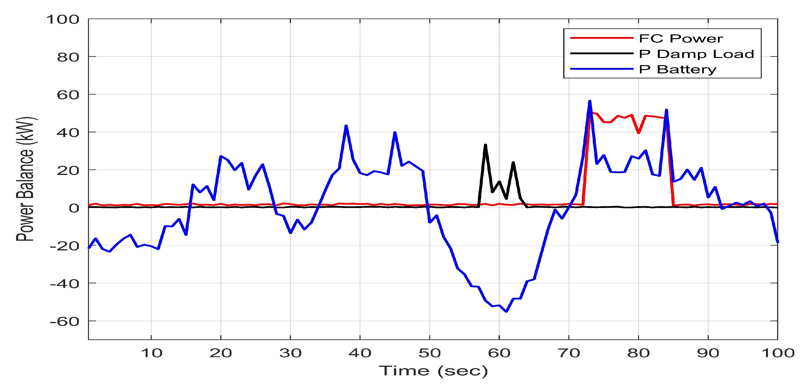
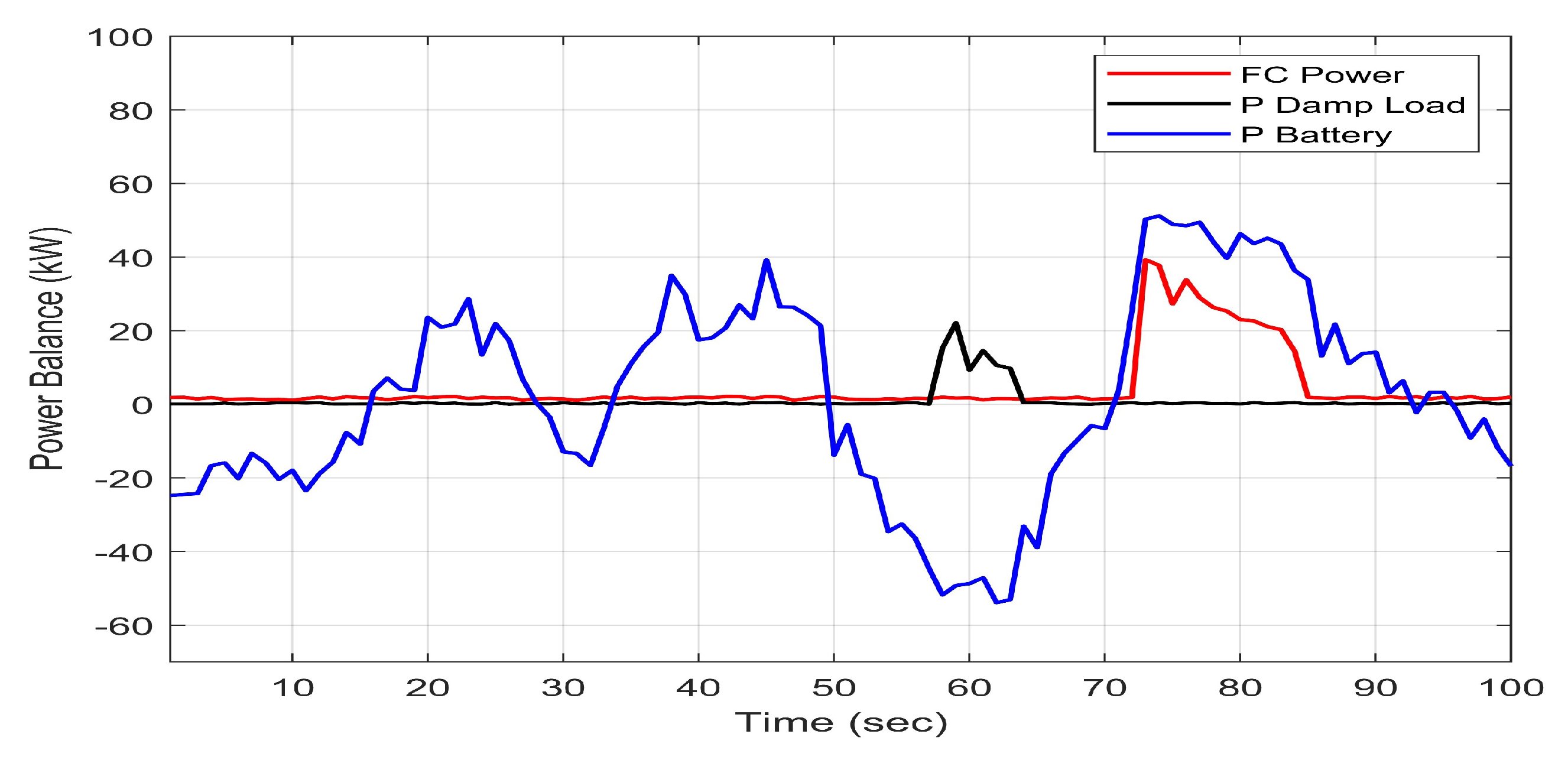
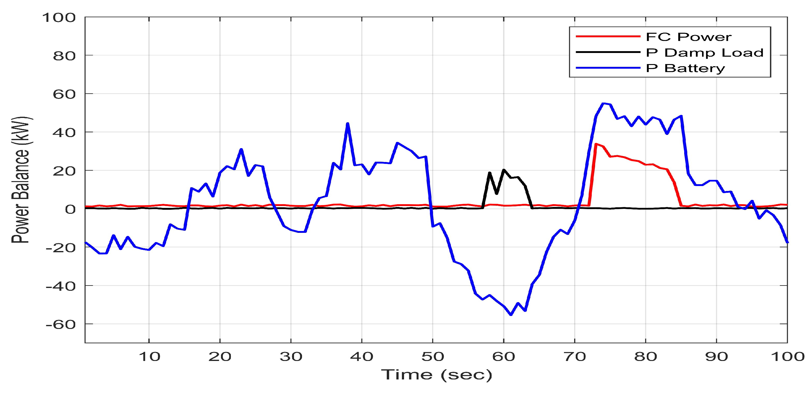
Let us preliminarily observe that both the optimized TS system and the optimized intuitionistic TS system showed significant performance by covering the demand represented by the load, whatever the operating conditions. This is because the number of rules and their structuring in terms of localization and shape of the FMFs are obtained with deep-learning techniques directly from real data, without relying on expert knowledge, considerably reducing the risk of neglecting any MG behaviors. However, some differences in behavior regarding both the use of the battery and the FC should be highlighted. In all the cases discussed, it is clear that the battery is charged both at the beginning of the day and in the early afternoon hours, so that when the load is less than the energy production, the excess power is stored, also guaranteeing the stability of the bus by balancing the entire system. The battery discharge process occurs in the meridian period or when the generated power is not enough to cover the load (essentially due to the lack of solar energy). As in [
26], backup devices step in to share the missing power. As regards the FC, until late afternoon, its activation is negligible in all cases treated. However, using the Mamdani system, when the battery power drops, the FC is forced to deliver substantial amounts of power with consequent consumption of
. This phenomenon is significantly mitigated if both optimized TS systems work. In particular, the intuitive approach offers a slight performance increase compared to the optimized TS, but without considering the uncertainty in the FMFs. Finally, the excess power is well recovered for hydrogen production (for details, see
Figure 13,
Figure 14 and
Figure 15).
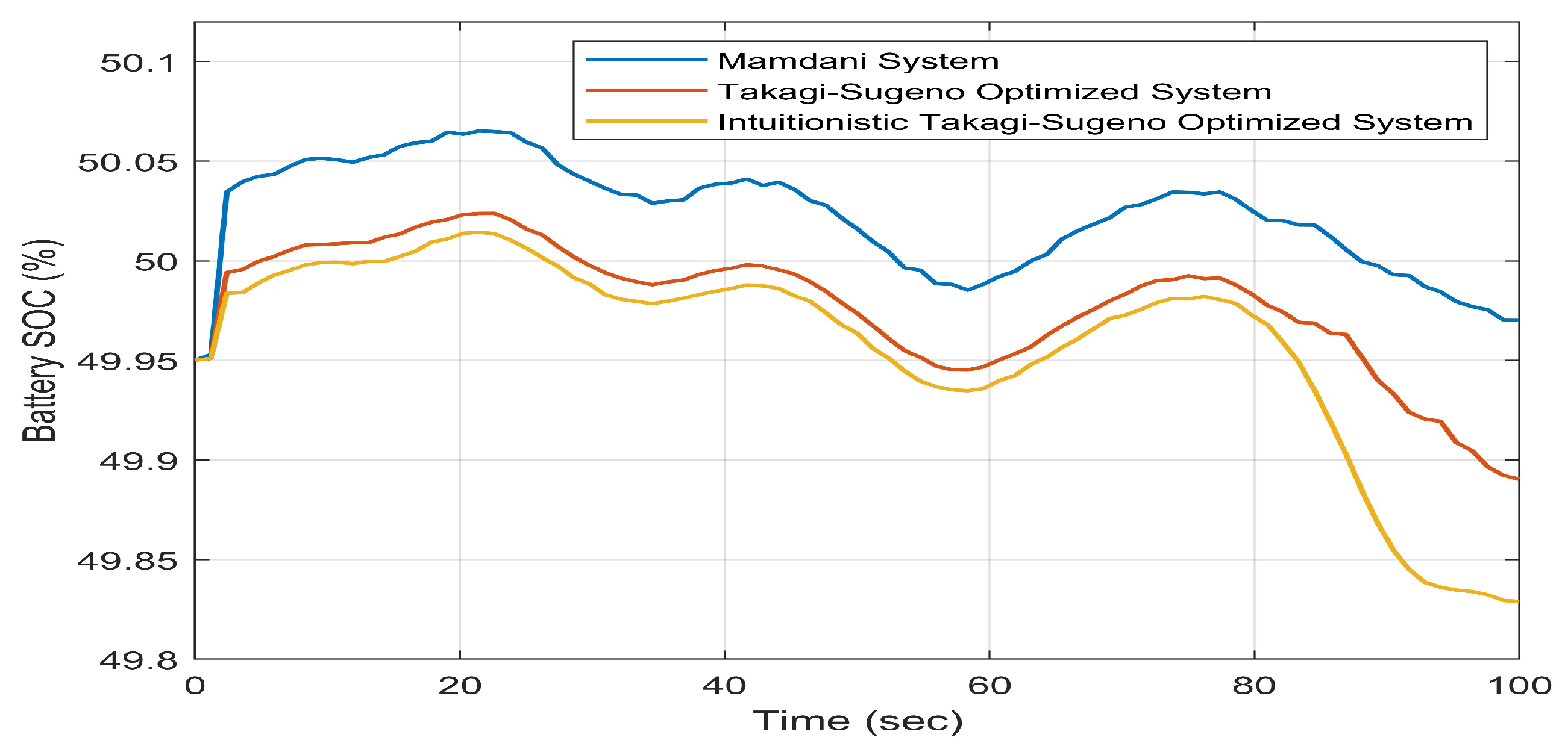
Regarding the percentage variation of the battery SOC over 24 h, as in [
26], there are no large differences in performance when the fuzzy approach used varies. This is due to the switching mode implemented in the simulation phase, as is done in [
26]. However, Mamdani’s approach confirms a consistent charging–discharging trend of the battery, as already highlighted in [
26], since the use of energy coming from the FC is more marked compared to both implemented TS systems, which have better performance in SoC percentages (see
Figure 16). This is highlighted even more by the fact that the air and hydrogen consumption of the FC stands at around 111.14 Ipm for the Mamdani system while for the optimized and intuitionistic TS systems they stand at around 44.26 Ipm and 39.18 Ipm, highlighting that the TS approaches proposed require less battery consumption.
Finally, it is worth underlining the fact that the optimization procedures concern exclusively the localization of the membership functions (and, in the case of the intuitionistic approach, of the non-membership functions and consequent hesitation functions). It follows that the runner tiles of each fuzzy approach used, being all rules of the same structure, have completely comparable execution times (and, in any case, are dependent on the type of workstation used).


